Unconditionally Dynamically Consistent Numerical Methods with Operator-Splitting for a Reaction-Diffusion Equation of Huxley’s Type

Abstract

The efficiency of various numerical methods for solving Huxley’s equation—which includes a diffusion term and a nonlinear reaction term—is investigated. Conventional explicit finite difference algorithms often suffer from severe stability limitations and can yield unphysical concentration values. In this study, we collect a range of stable, explicit time integration methods of first to fourth order, originally developed for the diffusion equation, and design treatments of the nonlinear term which ensure that the solution remains within the physically meaningful unit interval. This property, called dynamical consistency, is analytically proven and implies unconditional stability. In addition to this, the most effective ones are identified from the large number of constructed method combinations. We conduct systematic tests in one and two spatial dimensions, also evaluating computational efficiency in terms of CPU time. Our results show that higher-order schemes are not always the most efficient: in certain parameter regimes, second-order methods can outperform their higher-order counterparts.

1. Introduction

In this work, we study Huxley’s equation [1] in the following form

$${\displaystyle \frac{\mathsf{\partial }u}{\mathsf{\partial }t}}=\alpha {\nabla }^{2}u+\beta u^2\left(1-u\right)$$

(1)

where α and β are non-negative real numbers. The initial and boundary conditions will be described later in this paper. A slightly generalized form of (1), which is often called the Huxley equation [2], is

$${\displaystyle \frac{\mathsf{\partial }u}{\mathsf{\partial }t}}=\alpha {\nabla }^{2}u+\beta u\left(1-u\right)\left(u-\gamma \right),$$

(2)

where $\gamma \in \left[0,1\right]$, and we always take $\gamma =0$ in this paper. Equation (2) is sometimes called the FitzHugh–Nagumo equation [3], but more general equations also appear under that name. These equations are members of the important family of nonlinear diffusion-reaction partial differential equations (PDEs) used to model various phenomena in biology and physics. For example, it was demonstrated [1] that equations with a cubic reaction term, such as (1) or (2), are useful to describe the propagation of a new, useful recessive gene in a population which reproduces itself sexually. They are also suitable [4] to model nerve pulse propagation in biological tissues, where the equation describes the transmission of electrical signals along nerve fibers. We note that Equation (1) is similar to Fisher’s equation

$${\displaystyle \frac{\mathsf{\partial }u}{\mathsf{\partial }t}}=\alpha {\nabla }^{2}u+\beta u\left(1-u\right),$$

(3)

where the nonlinear term is only quadratic, and thus it is nonlinear to a lesser degree than Huxley’s equation.

It is well known that the correct solution of the diffusion or heat equation always adheres to the minimum and maximum principles, which reflect the second law of thermodynamics. The minimum principle guarantees that the equation does not produce negative values if the initial and boundary values are non-negative, which is called the positivity-preserving property. When there is a reaction or other source term in the equation, these criteria are not always applicable. However, the reaction term in Equation (1) has the special property that its limit value is zero both in the $u\to 0$ and the $u\to 1$ cases. Therefore, a similar principle, which will be called dynamical consistency, is valid: if the initial and boundary values of the u variable are in the unit interval, then u remains in this interval for any non-negative values of the parameter β. We note that this property holds for Equation (2) for $\gamma \in \left[0,1\right]$, but the dynamics of the time development strongly depend on the value of γ. For example, if γ is 0, then $u\equiv 1$ is the only stable steady state while $u\equiv 0$ is an unstable steady state. On the other hand, if $\gamma =1$, then the cases are the other way around.

Unfortunately, the plausible requirement that the applied numerical schemes should preserve this quality of the solution is rarely guaranteed, with a very few exceptions, such as a few exact or nonstandard finite difference (NSFD) schemes [5]. Due to the discretization, the solutions produced by standard finite difference methods can contain meaningless (negative or two large) values, causing oscillations and even numerical instabilities. The widespread explicit methods have a severely limited stability region [6], even for the pure diffusion- or heat equation: the solution is expected to blow up if the time-step size exceeds the so-called CFL (Courant–Friedrichs–Lewy) limit. In the case of a heterogeneous media, one has a space-dependent α coefficient [7], and thus the CFL limit for the explicit methods is rather small, and the stiffness ratio is high. The problem of restricted stability persists in the case of the most frequent explicit methods, which work via the method of lines: the PDE is first spatially discretized, and then the obtained system of ordinary differential equations (ODEs) is solved by a well-established ODE solver. If this solver is the forward Euler method, then one has the FTCS (forward time central space) scheme, the stability limit of which will be used in this work to characterize the difficulty level of the problem. Higher-order methods, such as the strong stability-preserving Runge–Kutta (RK) methods [8,9], also suffer from stability issues.

Implicit methods, such as the so-called shifted airfoil collocation method applied by Anjuman et al. [10] for nonlinear drift-diffusion-reaction equations, have better stability properties, although sometimes step-size limitations can be required [11]. However, they demand the solution of a nonlinear algebraic equation system, which can be time- and memory-consuming if the size of the equation system is large. In spite of this, diffusion-reaction equations are often solved by implicit methods. Moreover, the diffusion term is sometimes even treated exactly [12] in the case of a stiff problem.

El-Danaf et al. solved the time-fractional Huxley equation by the variational iteration and the Adomian decomposition methods [13]. A semi-analytical reduced differential transform method (RDTM) [14] was utilized by Patel and Dhodiya. Bai et al. employed a physics-informed neural network (PINN) and an improved PINN, called IPINN [15]. They observed that the latter one more accurately reproduces the different dynamic behaviors of the equation. However, this new method still has a limitation that, with the increase in the order and the increase in the nonlinear term of the PDEs, it cannot obtain the proper numerical solution of the PDEs. Manaa and Sabawi [16] used the explicit (Euler) and the Crank–Nicolson (CN) methods to solve Equation (2). They observed that the explicit method is faster, but as expected, the CN scheme is more accurate and does not suffer from serious stability issues. Dynamically consistent or at least unconditionally positive methods to solve these or similar equations are investigated by a few scholars [17,18,19]. Macías-Díaz constructed a finite-difference numerical scheme for the Burgers–Huxley equation with dynamical consistency [20]. However, he used the explicit Euler time-discretization for the diffusion term, and thus his method possesses good properties only for small time-step sizes below the CFL number. The same is true for the positivity-preserving scheme proposed by Chertock and Kurganov [21] for advection-diffusion-reaction equation-system modeling chemotaxis/haptotaxis problems, the nonstandard finite difference schemes (NSFDs) of the group of Appadu [3,22,23] for the Fisher and Nagumo equations, and that of Songolo [24] and Chapwanya et al. [25] for cross-diffusion equations.

Our goal in this work is to investigate numerical schemes which are unconditionally stable and dynamically consistent. A similar study, but with a smaller number of methods, has been carried over in our recent work [26] for Fisher’s equation. We also constructed efficient methods for Huxley’s equation [27], but none of them had the property of dynamical consistency. For us, the word unconditional always means that the desirable properties hold for arbitrary non-negative coefficients α and β, arbitrary positive time-step sizes, and arbitrary mesh for space discretization. Therefore, in Section 2, the spatial discretization of Equation (1) is considered not only in the simplest, one-dimensional case, but in a very general case as well. Since operator-splitting is applied, first the treatment of the diffusion term and then the nonlinear reaction term is discussed. In Section 3, we first briefly recall 13 numerical algorithms which, when applied to the pure diffusion equation, follow the maximum and minimum principle. Then, in Section 4, five different treatments of the reaction term are constructed, and the dynamical consistency property, valid for all of the $5\times 13=65$ algorithm combinations, is analytically proved. In Section 5, we perform the verification using an analytical reference solution. Based on this, we immediately exclude one of the five treatments of the Huxley term from further examination. After this, via the Strang-splitting technique, we construct further versions of the methods, and we test the obtained algorithm combinations. The results of these tests help us to select the 28 combinations which we think are worth testing further. In Section 6, the performance of these 28 combinations with running-time measurements is carried out for two different two-dimensional systems to select the top nine methods. The last three further numerical case studies in Section 7 use only these nine combinations. There are two parameter sweeps for the nonlinear coefficient β (with a stiff and a non-stiff system) and one sweep for the stiffness ratio. The final conclusions and recommendations are summarized in Section 8.

2. The Spatial Discretization of the Diffusion Equation Using Uniform and Non-Uniform Meshes

In this section, the pure diffusion equation is discretized. First, the simple equidistant discretization $x_i=x_0+i\Delta x, i=1,\dots , N,N\Delta x=L$ of the interval $x\in \left[x_0,x_N=x_0+L\right]\subset ℝ$ is constructed. The well-known central difference approximation is applied to the second spatial derivatives leading to the ODE system

$${\displaystyle \frac{d{u}_i}{dt}}={\displaystyle \frac{\alpha }{\Delta x^2}}\left(u_{i-1}-2u_i+u_{i+1}\right)$$

(4)

for the nodes $i=1,\dots ,N-1$. A matrix denoted by M is defined as containing a lot of zeros and the following nonzero elements:

$$m_{ii}=-{\displaystyle \frac{2\alpha }{\Delta x^2}}(1<i<N), m_{i,i+1}={\displaystyle \frac{\alpha }{\Delta x^2}}(1\le i<N), m_{i,i-1}={\displaystyle \frac{\alpha }{\Delta x^2}}(1<i\le N).$$

(5)

In the one-dimensional case, M is tridiagonal. The first and the last rows depend on the boundary conditions (BCs). For example, the time development of the first and the last nodes will be determined by the analytical solution in Section 5 in the case of Dirichlet BCs. Thus, the appropriate elements of M can be set to zero since they will not be used. The ODE system (4) may be rephrased in the following matrix form:

$${\displaystyle \frac{dU}{dt}}=MU,$$

(6)

where $U={\left(u_0,\dots ,u_N\right)}^{\mathrm{T}}$. We are going to deal with more general problems where the material and geometrical properties of the studied system have a space dependence. The space discretization, and later, the methods should be extended to reflect this level of generality. If α (which is a property of the media) depends on the space variable, but we are still in 1D, the PDE

$${\displaystyle \frac{\mathsf{\partial }u}{\mathsf{\partial }t}}={\displaystyle \frac{\mathsf{\partial }}{\mathsf{\partial }x}}\left(\alpha \left(x\right){\displaystyle \frac{\mathsf{\partial }u}{\mathsf{\partial }x}}\right)$$

can be used. In this equation, it is possible to simultaneously discretize the function α and $\mathsf{\partial }u/\mathsf{\partial }x$, which gives

$${\left.{\displaystyle \frac{\mathsf{\partial }u}{\mathsf{\partial }t}}\right|}_{x_i}={\displaystyle \frac{1}{\Delta x}}\left[\alpha \left(x_i-{\displaystyle \frac{\Delta x}{2}}\right){\displaystyle \frac{u(x_i-\Delta x)-u(x_i)}{\Delta x}}+\alpha \left(x_i+{\displaystyle \frac{\Delta x}{2}}\right){\displaystyle \frac{u(x_i+\Delta x)-u(x_i)}{\Delta x}}\right].$$

The average diffusivity between cell i and its (left) neighbor may be denoted by ${\alpha }_{i,i-1}$, which, in practice, can be approximated by its value between these two nodes. With this, we have

$${\displaystyle \frac{d{u}_i}{dt}}={\displaystyle \frac{1}{\Delta x}}\left({\alpha }_{i,i+1}^n{\displaystyle \frac{u_{i+1}-u_i}{\Delta x}}+{\alpha }_{i,i-1}^n{\displaystyle \frac{u_{i-1}-u_i}{\Delta x}}\right),$$

which is a generalized form of Equation (2). Our goal is to introduce a very flexible resistance–capacitance model by considering cells instead of nodes. These cells have finite volumes, which can be given as $V_i=\Delta x$ in the one-dimensional equidistant case. We have to interject that our methods are not finite volume methods (FVMs), but they are much closer to the finite difference methods. In the case of the simplest diffusion, the capacity of each cell equals its volume: $C_i=V_i=\Delta x$. The resistance between two cells can be given simply as $R_{i,i+1}=R_{i+1,i}={\displaystyle \frac{\Delta x}{{\alpha }_{i,i+1}}},i=1,\dots ,N-1$. Using these, one can obtain the ODE system for the time derivative of each cell variable u in one spatial dimension:

$${\displaystyle \frac{d{u}_i}{dt}}={\displaystyle \frac{u_{i-1}-u_i}{R_{i,i-1}{C}_i}}+{\displaystyle \frac{u_{i+1}-u_i}{R_{i,i+1}{C}_i}}.$$

(7)

Equation (7) can be written in the same matrix form as (6), where the non-diagonal elements have the form $m_{i,i-1}={\displaystyle \frac{1}{R_{i,i-1}{C}_i}}$ and $m_{i,i+1}={\displaystyle \frac{1}{R_{i,i+1}{C}_i}}$, while the diagonal elements are the negative sum of the non-diagonal ones: $m_{i,i}=-{\displaystyle \frac{1}{R_{i,i-1}{C}_i}}-{\displaystyle \frac{1}{R_{i,i+1}{C}_i}}$.

We will also work in two spatial dimensions, where the numbering of the cells begins along the x-directional (horizontal) rows running from 1 to $N_x$, then along the x axis again from $N_x+1$ to $2N_x$, and so on. The ODE system (7) can now be straightforwardly generalized to the case with two spatial dimensions:

$${\displaystyle \frac{d{u}_i}{dt}}={\displaystyle \frac{u_{i-1}-u_i}{R_{i,i-1}{C}_i}}+{\displaystyle \frac{u_{i+1}-u_i}{R_{i,i+1}{C}_i}}+{\displaystyle \frac{u_{i-Nx}-u_i}{R_{i,i-Nx}{C}_i}}+{\displaystyle \frac{u_{i+Nx}-u_i}{R_{i,i+Nx}{C}_i}}={\displaystyle \sum _{j\ne i}\frac{u_j-u_i}{R_{i,j}{C}_i}}.$$

(8)

One can find further details on the discretization via this resistance–capacitance model, e.g., in [28,29].

When performing numerical experiments in 2D, we always consider zero Neumann BCs. These will be implemented in the RC model very simply: the appropriate resistances are considered to be infinity, which means that the matrix elements responsible for conduction across the boundaries vanish. In this case, the system matrix M has a zero eigenvalue corresponding to the conserved quantity. All other eigenvalues are negative, which is true without exception for the case of zero Dirichlet BCs. Let us denote by λ_MIN and λ_MAX the eigenvalues with the (nonzero) smallest and largest absolute values, respectively. The stiffness ratio of the problem is usually defined as SR = λ_MAX/λ_MIN. On the other hand, the CFL limit $h_{MAX}^{RK1}=\left|2/{\lambda }_{MAX}\right|$ accurately gives the maximum time-step size that the explicit Euler (first-order explicit RK) scheme can employ for the pure (linear) diffusion problem (4), (7), or (8). From stability polynomial analysis, one can obtain similar time-step size thresholds for higher-order explicit RK methods. For example, for the second-, third-, and fourth-order RK schemes, one has $h_{MAX}^{RK2}=h_{MAX}^{RK1}$, $h_{MAX}^{RK3}\approx 1.256\cdot h_{MAX}^{RK1}$, and $h_{MAX}^{RK4}\approx 1.392\cdot h_{MAX}^{RK1}$, respectively. If the user exceeds these limits, the solutions blow up due to the instability. The two numbers SR and $h_{MAX}^{RK1}$ characterize the degree of difficulty of the linear part of the problem. We have to stress once more that the unconditionally stable methods used in this work have no CFL limits, as we will see soon.

3. The 13 Examined Methods for the Diffusion Equation with the Convex-Combination Property

The numerical algorithms for the linear diffusion equation are briefly described here, and the treatments of the Huxley term will be presented in the next section. The time variable is always discretized uniformly using the following notations:

$$t^n=t^{\mathrm{ini}}+nh, t\in \left[t^{\mathrm{ini}},t^{\mathrm{fin}}\right], n=1,\dots ,T, hT=t^{\mathrm{fin}}-t^{\mathrm{ini}}$$

In the special case of an equidistant one-dimensional mesh with constant diffusivity α, the mesh ratio is usually defined as $r={\displaystyle \frac{\alpha h}{\Delta x^2}}=-{\displaystyle \frac{m_{ii}h}{2}}>0, 0<i<N-1$. Since the general case of space-dependent α and non-uniform mesh contains this special case, only the generalized formula of the numerical algorithms is presented. Let us define the quantity

$$r_i=h{\displaystyle \sum _{j\ne i}\frac{1}{C_i{R}_{ij}}=-}h{m}_{ii},$$

(9)

which is the generalization of the mesh ratio r, since, in the 1D special case, $r_i=2r$. We also introduce a quantity to collect the effect of the neighbors of the cell with index i as follows:

$$A_i=h{\displaystyle \sum _{j\ne i}\frac{u_j^n}{C_i{R}_{ij}}=}h{\displaystyle \sum _{j\ne i}{m}_{ij}{u}_j^n}$$

In the special 1D case, $A_i=r\left(u_{i-1}^n+u_{i+1}^n\right), \mathrm{hence} {\displaystyle \frac{A_i}{r_i}}={\displaystyle \frac{u_{i-1}^n+u_{i+1}^n}{2}}$. Using these relations, one can easily obtain the formulas applicable in the 1D special case from their generalized variants. The application of the methods is very similar to that of the standard explicit Euler or RK methods, with only the formulas used being different. For the two exceptions, we will display a flowchart to make understanding easier.

1. The simplest method we use is called the unconditionally positive finite difference (UPFD) scheme. This was introduced by Chen-Charpentier and Kojouharov [17] for the linear diffusion-advection-reaction equation discretized by an equidistant mesh. We do not have the advection term, and we adapt the formula to our general Equations (7) and (8) as follows:

$$u_i^{n+1}={\displaystyle \frac{u_i^n+A_i}{1+r_i}}$$

(10)

2. In the case of the CNe, or constant neighbor method [30], the positive $r_i$ quantities containing the time-step size are in the exponent with a negative sign:

$$u_i^{n+1}=u_i^n\cdot e^{-r_i}+{\displaystyle \frac{A_i}{r_i}}\left(1-e^{-r_i}\right)$$

(11)

This ensures the outstanding stability properties of the methods built on this CNe formula.

In this work, we test two different odd–even hopscotch-type algorithms. To do this, we need a special checkerboard-like characterization of the cells, where the neighbors of the cells with the label ‘odd’ are labeled as ‘even’ and vice versa. The time-marching for the u values goes alternately for the set of the odd and the even cells. When one set is calculated, the latest values of the neighbors $u_{i\pm 1}, u_{i\pm Nx}$ belonging to the other set are always used in the formula for $A_i$. We note that only one function evaluation is required per cell per time step, so these solvers are quite fast.

3. OOEH-CNe method: The original odd–even hopscotch time-space structure is applied, as one can see in the flowchart in Figure 1. It means that the odd values are refreshed first, and then the even values. However, after each time step, the odd–even labels are interchanged. The length of the time steps is always the full h, and the CNe formula (11) is employed in each stage.

4. The LH-CNe algorithm: The leapfrog–hopscotch (LH) structure contains time steps with length not only with integer h, but with h/2. The solution begins with a half time step for, e.g., the odd cells, after which full-length time steps are allowed for the set of the even and the odd cells, strictly alternately. This goes until we reach the last time step, which must have the length of h/2 for the set of the odd cells again to precisely reach the final time $t^{\mathrm{fin}}$. The LH-CNe method investigated in this paper always employs the CNe formula (11) with the appropriate full or half time-step size.

5. The CpC method [29] first calculates new predictor u values applying the CNe formula (11), but with a halved time step:

$$u_i^{\mathrm{pred}}=u_i^n{e}^{-r_i/2}+{\displaystyle \frac{A_i}{r_i}}\left(1-e^{-r_i/2}\right)$$

(12)

These predictor values are used to obtain the new

$$A_i^{\mathrm{pred}}=\Delta t{\displaystyle \sum _{\mathrm{j}\ne \mathrm{i}}\frac{u_j^{\mathrm{pred}}}{C_i{R}_{ij}}}$$

(13)

quantities. Then the second, corrector stage constitutes a full time step with (11) again:

$$u_i^{n+1}=u_i^n\cdot e^{-r_{\mathrm{i}}}+{\displaystyle \frac{A_i^{\mathrm{pred}}}{r_i}}\left(1-e^{-r_{\mathrm{i}}}\right)$$

(14)

6. The LNe (or sometimes LNe2, meaning two-stage linear-neighbor) algorithm is a predictor–corrector method [30], too. The first stage uses the above given CNe formula with full time-step size, and it gives the new $u_{\mathrm{i}}^{\mathrm{pred}}$ predictor values. Using these, one can use Equation (13) and then calculate the corrector values:

$$u_i^{n+1}=u_i^n{e}^{-r_i}+\left(A_i-{\displaystyle \frac{A_i^{\mathrm{pred}}-A_i}{r_i}}\right){\displaystyle \frac{1-e^{-r_i}}{r_i}}+{\displaystyle \frac{A_i^{\mathrm{pred}}-A_i}{r_i}}$$

(15)

7-8-9. The corrector values given by Equation (15) are used to calculate $A_i^{\mathrm{pred}}$ with (13) again, and thus one repeats (15) to obtain refined u values. This increases the total number of stages in one time step to three, and hence, the seventh algorithm is called LNe3 [30]. This iteration can be continued to obtain the LNe4 (LNe5) method, which has four (five) stages altogether. These are obtained by repeating (13) and (15). These iterations, although they yield slightly larger accuracy, unfortunately do not improve the order.

10. The three-stage constant-linear-quadratic neighbor (CLQ) method [31] is a bit more complicated than the previous ones, since it also employs the quadratic-neighbor approximation. Its first two stages are similar to those of the LNe algorithm: $A_i$ is calculated at the beginning of the first stage, and then one full-size time step with (10) is performed. After using (12), the LNe stage (15) comes with a full as well as a half-length time step, to obtain the sets $u_i^{\mathrm{L}}$ and $u_i^{\mathrm{L}\raisebox{1ex}{$1$}\!\left/ \!\raisebox{-1ex}{$2$}\right.}$, respectively. Using these, one can repeat Equation (13) to calculate $A_i^{\mathrm{pred},\mathrm{L}}$ and $A_i^{\mathrm{pred},\mathrm{L}\raisebox{1ex}{$1$}\!\left/ \!\raisebox{-1ex}{$2$}\right.}$, both without dividing h by 2 in (13). Two new quantities, $S_i=4A_i^{\mathrm{pred},\mathrm{L}\raisebox{1ex}{$1$}\!\left/ \!\raisebox{-1ex}{$2$}\right.}-A_i^{\mathrm{pred},\mathrm{L}}-3A_i$ and $W_i=2\left(A_i^{\mathrm{pred},\mathrm{L}}-2A_i^{\mathrm{pred},\mathrm{L}\raisebox{1ex}{$1$}\!\left/ \!\raisebox{-1ex}{$2$}\right.}+A_i\right)$, must then be calculated. The new u values are given by

$$u_i^{\mathrm{Q}}=e^{-r_i}{u}_i^n+{\displaystyle \frac{1-e^{-r_i}}{r_i}}\left({\displaystyle \frac{2W_i}{r_i^2}}-{\displaystyle \frac{S_i}{r_i}}+A_i\right)+{\displaystyle \frac{\left(1-2/r_i\right)W_i+S_i}{r_i}}$$

(16)

11-12-13. We can add one more stage by using the values in (16). In this case, besides (16) at the third stage, the midpoint values must also be calculated by a similar formula:

$$u_i^{\mathrm{Q}\raisebox{1ex}{$1$}\!\left/ \!\raisebox{-1ex}{$2$}\right.}=e^{-r_i/2}{u}_i^n+{\displaystyle \frac{1-e^{-r_i/2}}{r_i}}\left({\displaystyle \frac{2W_i}{r_i^2}}-{\displaystyle \frac{S_i}{r_i}}+A_i\right)+{\displaystyle \frac{W_i}{4r_i}}-{\displaystyle \frac{W_i}{r_i^2}}+{\displaystyle \frac{S_i}{2r_i}}$$

(17)

Using these, one can calculate $A_i^{\mathrm{pred},Q}$ and $A_i^{\mathrm{pred},Q\raisebox{1ex}{$1$}\!\left/ \!\raisebox{-1ex}{$2$}\right.}$ values by (12) at the fourth stage, with which one repeats the calculations of the third stage, including those of S and W. With these, one has four stages altogether, which constitute the CLQ2 algorithm. One can further repeat this iteration by re-calculating $A_i^{\mathrm{pred},Q}$ and $A_i^{\mathrm{pred},Q\raisebox{1ex}{$1$}\!\left/ \!\raisebox{-1ex}{$2$}\right.}$, then applying (16) and (17) again, etc. If one has three or four quadratic stages (five or six stages altogether), we call the obtained methods CLQ3 and CLQ4, respectively [31].

Properties of the methods when solving the space-discretized diffusion equation: The orders of temporal accuracy are the following: one for the UPFD and the CNe, two for the OOEH-CNe, LH-CNe, CpC, and LNe-LNe5, three for the CLQ, and four for the CLQ2-4. All of these algorithms are unconditionally stable when applied to the linear diffusion equation; therefore, the previously mentioned CFL limit cannot confine their stability. This outstanding stability comes from the following property.

Theorem 1.

If methods 1–13 solve the spatially discretized linear diffusion Equation (4), then the new $u_i^n$ values are the convex combinations of the initial values $u_j^0$. The statement is true in the case of the general Equation (7) or (8), when the 1–9 methods are applied.

These statements have been analytically proved in the original papers. According to all of the numerical tests, the convex combination property holds when the CLQ-CLQ4 algorithms solve the generalized Equations (7) and (8), but we have not been able to prove this analytically. Furthermore, the truncation errors of the methods for the linear diffusion equation are calculated in our previous paper [32].

4. The Operator-Splitting Treatments of the Nonlinear Term

During a time step, we independently take into account the effect of the linear diffusion term and the nonlinear Huxley term. The diffusion term is treated by the 13 methods listed in the previous subsection. After fully considering the diffusion term by those schemes, we obtain a concentration value $u_i^{\mathrm{diff}}$, which we temporarily denote as p for brevity. The reaction term is local and can be written into the form $\beta u^2-\beta u^3$. A very efficient way to take into account this nonlinear term is to solve the initial value problem

$$\left\{\begin{array}{l}{\displaystyle \frac{du}{dt}}=\beta u^2-\beta u^3,\\ u\left(t=0\right)=u_i^{\mathrm{diff}}=p, t\in \left[0,h\right]\end{array}\right.$$

(18)

analytically, as in [26]. However, we were not able to solve this, even with the help of Maple 18 software. Hence, we choose an approach which starts with a selective replacement of u by the p values in all twelve possible ways:

$$\begin{array}{c}\beta u^2-\beta u^3\\ \beta u^2-\beta u^{2}p\\ \beta u^2-\beta u{p}^2\\ \beta u^2-\beta p^3\end{array}\begin{array}{c} \beta up-\beta u^3\\ \beta up-\beta u^{2}p\\ \beta up-\beta u{p}^2\\ \beta up-\beta p^3\end{array}\begin{array}{c} \beta p^2-\beta u^3\\ \beta p^2-\beta u^{2}p\\ \beta p^2-\beta u{p}^2\\ \beta p^2-\beta p^3\end{array}$$

(19)

Three of these ways, namely, $\beta up-\beta u{p}^2$, $\beta up-\beta p^3$, and $\beta p^2-\beta u{p}^2$, can be considered as a kind of linearization, while the last one without u is the equivalent to the explicit Euler treatment. After inserting each of the expressions (19) into the right-hand side of (18), we try to solve the obtained initial value problems, for example,

$$\left\{\begin{array}{l}{\displaystyle \frac{du}{dt}}=\beta pu-\beta p{u}^2,\\ u\left(t=0\right)=u_i^{\mathrm{diff}}=p, t\in \left[0,h\right]\end{array}\right.$$

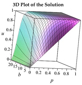
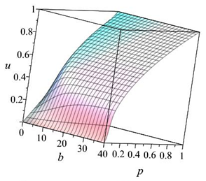
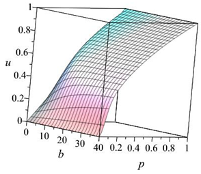
again analytically. If the solution is found, we first check whether the obtained analytical solutions guarantee dynamical consistency by plotting it as a function of p and $b:=\beta h$. We observed that there are two cases when there is no analytical solution, six cases (including the linearization $\beta up-\beta u{p}^2$) where the solution exists but it can be larger than one, and four cases when the solution is in the unit interval. These latter four cases will be used to treat the nonlinear term, and they are listed in the following Table 1.

Table 1. Four treatments of the nonlinear term.

Treatment	Substitution	Solution	3D Plot of the Solution
t1	$\beta up-\beta u^{2}p$	$u\left(h\right)={\displaystyle \frac{p}{p+\left(1-p\right)e^{-pb}}}$ or $$u_i^{n+1}={\displaystyle \frac{u_i^{\mathrm{diff}}}{u_i^{\mathrm{diff}}+\left(1-u_i^{\mathrm{diff}}\right)e^{-u_i^{\mathrm{diff}}\beta t}}}$$ (20)
t2	$\beta up-\beta u^3$	$u\left(h\right)={\displaystyle \frac{p}{\sqrt{p+\left(1-p\right)e^{-2pb}}}}$ or $$u_i^{n+1}={\displaystyle \frac{u_i^{\mathrm{diff}}}{\sqrt{u_i^{\mathrm{diff}}+\left(1-u_i^{\mathrm{diff}}\right)e^{-2u_i^{\mathrm{diff}}\beta t}}}}$$ (21)
t3	$\beta p^2-\beta u^{2}p$	$u\left(h\right)=\sqrt{p}\tan \mathrm{h}\left(b{p}^{3/2}+\mathrm{arctanh}\left(\sqrt{p}\right)\right)$ or $$\begin{array}{l}{u}_i^{n+1}=\sqrt{u_i^{\mathrm{diff}}}\tan \mathrm{h}\\ \left(\beta t{\left(u_i^{\mathrm{diff}}\right)}^{3/2}+\mathrm{arctanh}\left(\sqrt{u_i^{\mathrm{diff}}}\right)\right)\end{array}$$ (22)
t4	$\beta p^2-\beta u{p}^2$	$u\left(h\right)=1-\left(1-p\right)e^{-p^{2}b}$ or $$u_i^{n+1}=1-\left(1-u_i^{\mathrm{diff}}\right)e^{-{\left(u_i^{\mathrm{diff}}\right)}^2\beta t}$$ (23)

Table 1. Four treatments of the nonlinear term.

Treatment	Substitution	Solution	3D Plot of the Solution
t1	$\beta up-\beta u^{2}p$	$u\left(h\right)={\displaystyle \frac{p}{p+\left(1-p\right)e^{-pb}}}$ or $$u_i^{n+1}={\displaystyle \frac{u_i^{\mathrm{diff}}}{u_i^{\mathrm{diff}}+\left(1-u_i^{\mathrm{diff}}\right)e^{-u_i^{\mathrm{diff}}\beta t}}}$$ (20)
t2	$\beta up-\beta u^3$	$u\left(h\right)={\displaystyle \frac{p}{\sqrt{p+\left(1-p\right)e^{-2pb}}}}$ or $$u_i^{n+1}={\displaystyle \frac{u_i^{\mathrm{diff}}}{\sqrt{u_i^{\mathrm{diff}}+\left(1-u_i^{\mathrm{diff}}\right)e^{-2u_i^{\mathrm{diff}}\beta t}}}}$$ (21)
t3	$\beta p^2-\beta u^{2}p$	$u\left(h\right)=\sqrt{p}\tan \mathrm{h}\left(b{p}^{3/2}+\mathrm{arctanh}\left(\sqrt{p}\right)\right)$ or $$\begin{array}{l}{u}_i^{n+1}=\sqrt{u_i^{\mathrm{diff}}}\tan \mathrm{h}\\ \left(\beta t{\left(u_i^{\mathrm{diff}}\right)}^{3/2}+\mathrm{arctanh}\left(\sqrt{u_i^{\mathrm{diff}}}\right)\right)\end{array}$$ (22)
t4	$\beta p^2-\beta u{p}^2$	$u\left(h\right)=1-\left(1-p\right)e^{-p^{2}b}$ or $$u_i^{n+1}=1-\left(1-u_i^{\mathrm{diff}}\right)e^{-{\left(u_i^{\mathrm{diff}}\right)}^2\beta t}$$ (23)

We have an extra treatment, where the effect of the Huxley term is calculated using an approach which we call the “pseudo-implicit” trick [31]. In this case, we replace u on the right-hand side of (17) with not only the $u_i^{\mathrm{diff}}$ values but also the new, unknown value $u_i^{n+1}$ with the goal of eliminating the negative terms from the right-hand side of this formula. In this way, we obtain

$${\displaystyle \frac{u_i^{n+1}-u_i^{\mathrm{diff}}}{h}}=\beta {\left(u_i^{\mathrm{diff}}\right)}^2-\beta {\left(u_i^{\mathrm{diff}}\right)}^2{u}_i^{n+1}$$

(24)

This can be simply rearranged to take on a completely explicit form:

$$u_i^{n+1}={\displaystyle \frac{1+\beta h{u}_i^{\mathrm{diff}}}{1+\beta h{\left(u_i^{\mathrm{diff}}\right)}^2}}{u}_i^{\mathrm{diff}}.$$

(25)

This will be the fifth treatment of the Huxley term, denoted by PI. Using the short, temporary notations, it has the form

$$u\left(h\right)={\displaystyle \frac{1+bp}{1+b{p}^2}}p.$$

Lemma 1.

If $0\le p\le 1$, then  $p\le u\le 1$ holds for the following five different $u\left(h\right)$ functions

$$1. u={\displaystyle \frac{p}{p+\left(1-p\right)e^{-pb}}}$$

$$2. u={\displaystyle \frac{p}{\sqrt{p+\left(1-p\right)e^{-2pb}}}}$$

$$3. u=\sqrt{p}\tan \mathrm{h}\left(b{p}^{3/2}+\mathrm{arctanh}\left(\sqrt{p}\right)\right)$$

$$4. u=1-\left(1-p\right)e^{-p^{2}b}$$

$$5. u={\displaystyle \frac{1+bp}{1+b{p}^2}}p$$

for arbitrary $b>0$. Furthermore, if $b=0$, then $p=u$, and u is monotonously increasing with increasing b.

Proof. 

We clearly have $0\le p^2\le p\le \sqrt{p}\le 1$, $0\le 1-p\le 1$, and $0\le e^{-2pb}\le e^{-pb}\le 1$, which will be used below, when the five functions are individually examined, as follows.

1. The term $\left(1-p\right)e^{-pb}$ is non-negative, and thus the denominator $p+\left(1-p\right)e^{-pb}$ cannot be smaller than p; hence, $u\le 1$. On the other hand, the denominator is majorated by unity:

$$p+\left(1-p\right)e^{-pb}=e^{-pb}+p\left(1-e^{-pb}\right)\le e^{-pb}+\left(1-e^{-pb}\right)=1.$$

Therefore, the denominator cannot be larger than one, and thus $p\le u$.

2. Since $\sqrt{p}\ge p$, the same argument as in point 1 can be repeated for this denominator $\sqrt{p+\left(1-p\right)e^{-2pb}}$ as well.

3. Both $\sqrt{p}$ and the tanh function are majorated by one, and thus also their product; hence, $u\le 1$. Moreover, the tanh is a monotonously increasing function, and thus $\sqrt{p}\cdot \tan \mathrm{h}\left(b{p}^{3/2}+\mathrm{arctanh}\left(\sqrt{p}\right)\right)\ge \sqrt{p}\cdot \tan \mathrm{h}\left(\mathrm{arctanh}\left(\sqrt{p}\right)\right)=\sqrt{p}\cdot \sqrt{p}=p$, which implies $p\le u$.

4. Since $\left(1-p\right)e^{-p^{2}b}$ is non-negative, $u\le 1$. On the other hand,

$$u=1-\left(1-p\right)e^{-p^{2}b}=p{e}^{-p^{2}b}+\left(1-e^{-p^{2}b}\right)\ge p{e}^{-p^{2}b}+p\left(1-e^{-p^{2}b}\right)=p,$$

and thus, we obtain $p\le u\le 1$.

5. The denominator $1+b{p}^2$ cannot be greater than the numerator $1+bp$, and thus ${\displaystyle \frac{1+bp}{1+b{p}^2}}\ge 1\Rightarrow u\ge p$. Additionally,

$$1+b{p}^2\ge p+b{p}^2\Rightarrow u\le 1.$$

The last statements of the lemma can be immediately obtained by the $b=0$ substitution. □

Simple operator-splitting means that a time step starts with the treatment of the diffusion by any of the algorithms displayed in Section 3, and after that, the treatment of the nonlinear term following one of the five ways above is conducted as a substitutional step. On the other hand, Strang-splitting means that one of the operations (20)–(25) is performed once before and a second time after the calculation of the effect of diffusion, both with halved time-step sizes. This means that the substitution $h\to h/2$ must be performed in (20) –(25). Note that in the case of Strang-splitting, the first and the second formulas for the nonlinear term are not necessarily the same; i.e., the treatments (20)–(25) can be hybridized. For example, it is possible to perform (20) with a halved h before and (22) after any of the methods 1–13 for the diffusion term.

Theorem 2.

(The methods’ dynamical consistency) Suppose one applies Methods 1–13 combined with treatments (20)–(25) with or without Strang-splitting to Huxley’s Equation (1). If the initial and boundary values of the concentration are in the unit interval $u_i^0, u_0^n, u_N^n\in \left[0,1\right]$, then the calculated concentration values will also be in this interval, i.e., $u_i^n\in \left[0,1\right]$ for any values of the coefficients α > 0, β > 0 and time-step size h > 0. Furthermore, increasing β can yield only the increase, and never the decrease, of the concentration values.

Proof of Theorem 2.

Due to the operator-splitting strategy, the procedure of the numerical solution consists of performing steps which treat the diffusion term and the nonlinear term subsequently. Theorem 1 and Lemma 1 imply that none of these steps can yield any concentration value outside of the unit interval, which immediately gives the first statement.

The last statement of Lemma 1 means that increasing β can yield only the increase in the concentration values calculated by any of the nonlinear steps given in Table 1. The convex combination property in Theorem 1 means that the steps which treat the diffusion term calculate linear combinations of the $u_i^n$ values with coefficients in the unit interval $\left[0,1\right]$. The non-negativity of these coefficients implies that if the u values are increased in the nonlinear step due to increasing β, that can yield only increased values after the diffusion step as well. □

The first statement of Theorem 2 is analogous to the maximum and minimum principles being valid for the pure (linear) diffusion equation.

Corollary 1.

If the conditions of Theorem 2 hold, the numerical solution is unconditionally stable, since the difference between the true and the numerical solutions cannot be larger than 1.

We note that a small fraction of the statements of Theorem 2 have been published in our paper [31].

5. Verification in 1D

Now PDE (1) with $\mathsf{\alpha }=1$ is going to be solved in the domain $\left(x,t\right)\in \left[x_0,x_N\right]\times \left[t^{\mathrm{ini}},t^{\mathrm{fin}}\right]$. The analytical solution [1] (p. 34)

$$u^{\mathrm{exact}}(x,t)={\displaystyle \frac{e^{\sqrt{\frac{\beta }{2}}x+\frac{\beta }{2}t}}{e^{\sqrt{\frac{\beta }{2}}x+\frac{\beta }{2}t}+c}}$$

(26)

is used as the reference. The initial and the Dirichlet boundary conditions are obtained by evaluating this function at the time and space points belonging to the initial time $u\left(x,0\right)$, and with the boundaries $u\left(x_0,t\right), u\left(x_N,t\right)$, respectively. The maximum numerical errors are calculated by comparing the numerical solutions $u_{\mathrm{j}}^{\mathrm{num}}$ produced using the examined method with the analytical reference solution $u_{\mathrm{j}}^{\mathrm{ref}}$ at the final time $t^{\mathrm{fin}}$ using the formula

$$\mathrm{Error}(L_{\infty })=\underset{0\le \mathrm{j}\le N}{\max }\left|u_{\mathrm{j}}^{\mathrm{ref}}(t^{\mathrm{fin}})-u_{\mathrm{j}}^{\mathrm{num}}(t^{\mathrm{fin}})\right|.$$

(27)

The average error is very similar:

$$\mathrm{Error}(L_1)={\displaystyle \frac{1}{N}}{\displaystyle \sum _{0\le \mathrm{j}\le N}\left|u_{\mathrm{j}}^{\mathrm{ref}}(t_{\mathrm{fin}})-u_{\mathrm{j}}^{\mathrm{num}}(t_{\mathrm{fin}})\right|}.$$

The third type of error has an energy dimension in the case of the heat conduction equation, and hence we call it the energy error:

$$\mathrm{Error}(Energy)={\displaystyle \sum _{1\le j\le N}{C}_j\left|u_j^{\mathrm{ref}}(t^{\mathrm{fin}})-u_j^{\mathrm{num}}(t^{\mathrm{fin}})\right|}.$$

We would like to assess the error not only for a specific time-step size but also for a wide range of time-step sizes. Hence, we start using the maximum possible time-step size $h=t^{\mathrm{fin}}-t^{\mathrm{ini}}$, calculate the errors defined above, and then repeat this calculation for subsequently decreasing time-step sizes. The time-step size is always divided by two, and the total number of different time-step sizes is denoted by P. We calculate the average of the logarithm of the obtained errors, which will be called the aggregated error (AgE). In the case of the maximum errors, it is given by the following formula

$$\mathrm{AgE}(L_{\infty })={\displaystyle \frac{1}{P}}{\displaystyle \sum _{k=1}^P\log \left(\mathrm{Error}(L_{\infty })\right)},$$

(28)

where the summation is going for the different time-step sizes. The final step is to calculate the average of the three different AgE errors:

$$\mathrm{AgE}={\displaystyle \frac{1}{3}}\left(\mathrm{AgE}(L_{\infty })+\mathrm{AgE}(L_1)+\mathrm{AgE}(Energy)\right).$$

(29)

Note that when the AgE is negative with a large absolute value, the method is very accurate. In this section, we calculated the aggregated error for P = 13 different time-step sizes for all the studied methods.

We perform two case studies using the analytical solution (26), with completely different parameter values.

Case Study 1: Medium nonlinear coefficient, equidistant mesh

PDE (1) is discretized on the $x_0=0, x_{N=200}=4, t^{\mathrm{ini}}=0.00, t^{\mathrm{fin}}=1.3$ domain using $\Delta x=0.02$ space step size. The nonlinear coefficient is $\beta =4.3$, while c = 1 in Equation (26).

Case Study 2: Large nonlinear coefficient, non-equidistant mesh

The equation is solved on the $\left[0,1.4416\right]$ interval with $t^{\mathrm{ini}}=0.1, t^{\mathrm{fin}}=0.29$. A non-equidistant spatial mesh is used with slowly increasing cell diameters from $\Delta x_1=0.002$ to $\Delta x_{400}=0.0052$. The nonlinear coefficient is quite large, $\beta =23.7$, and c = 3.6.

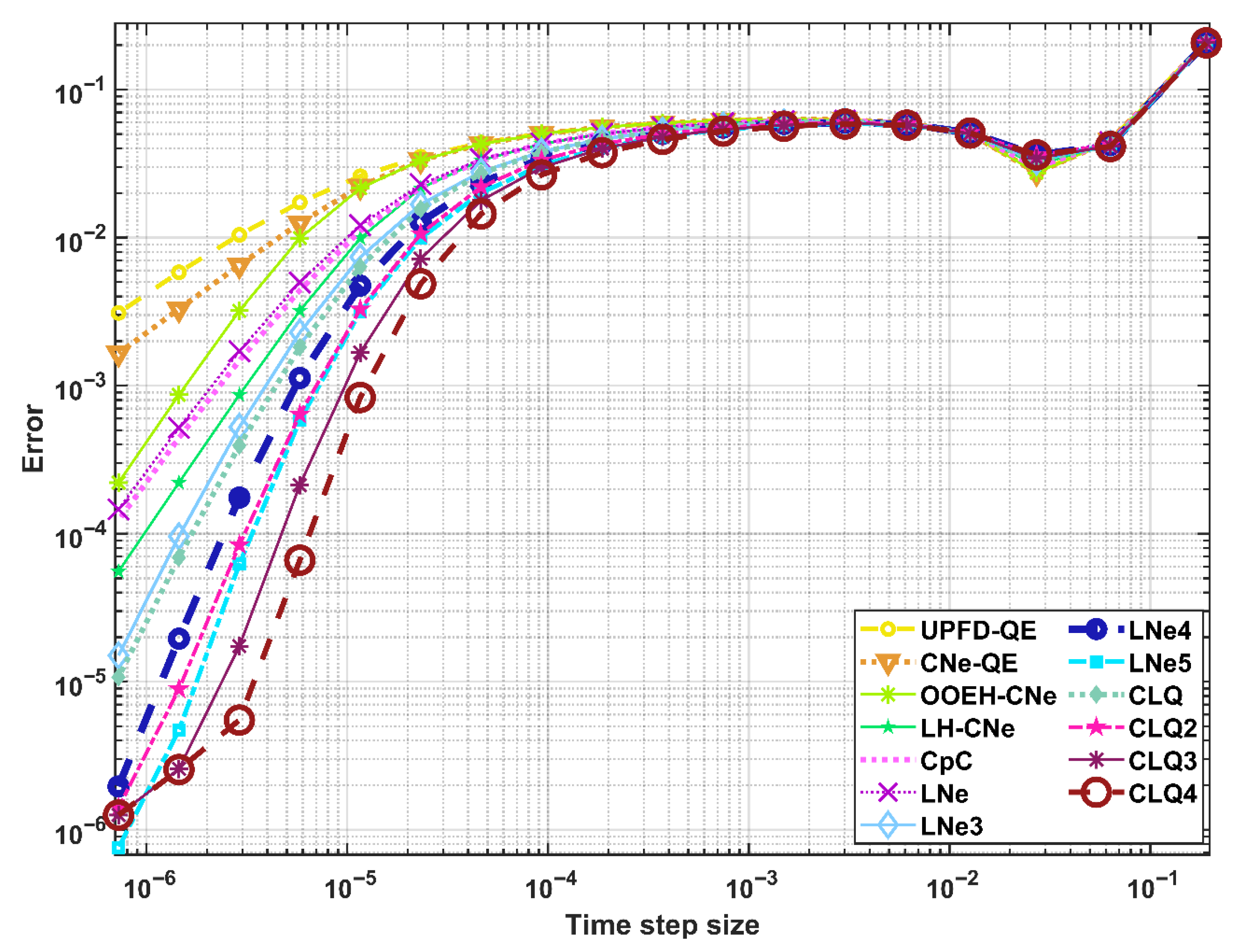
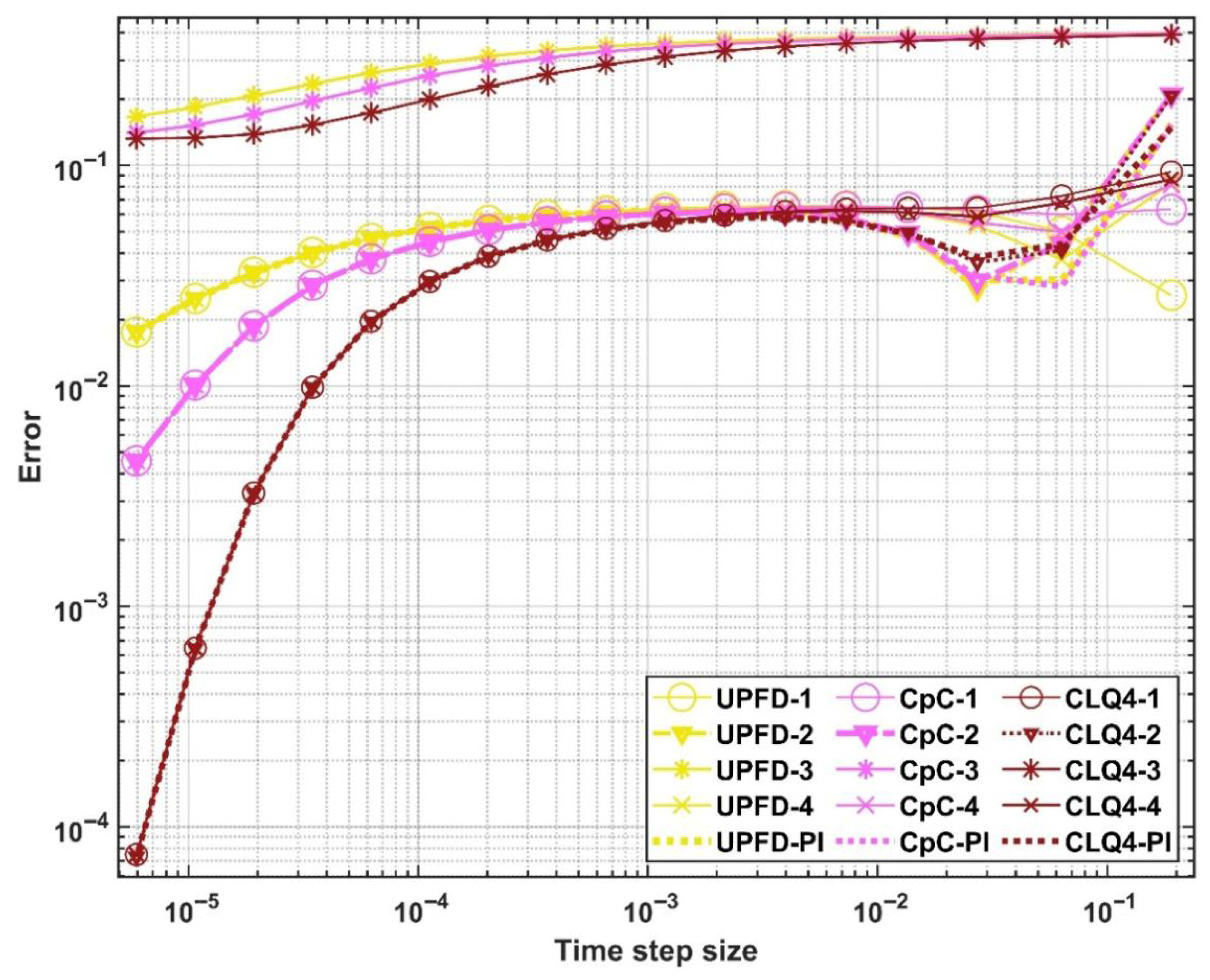
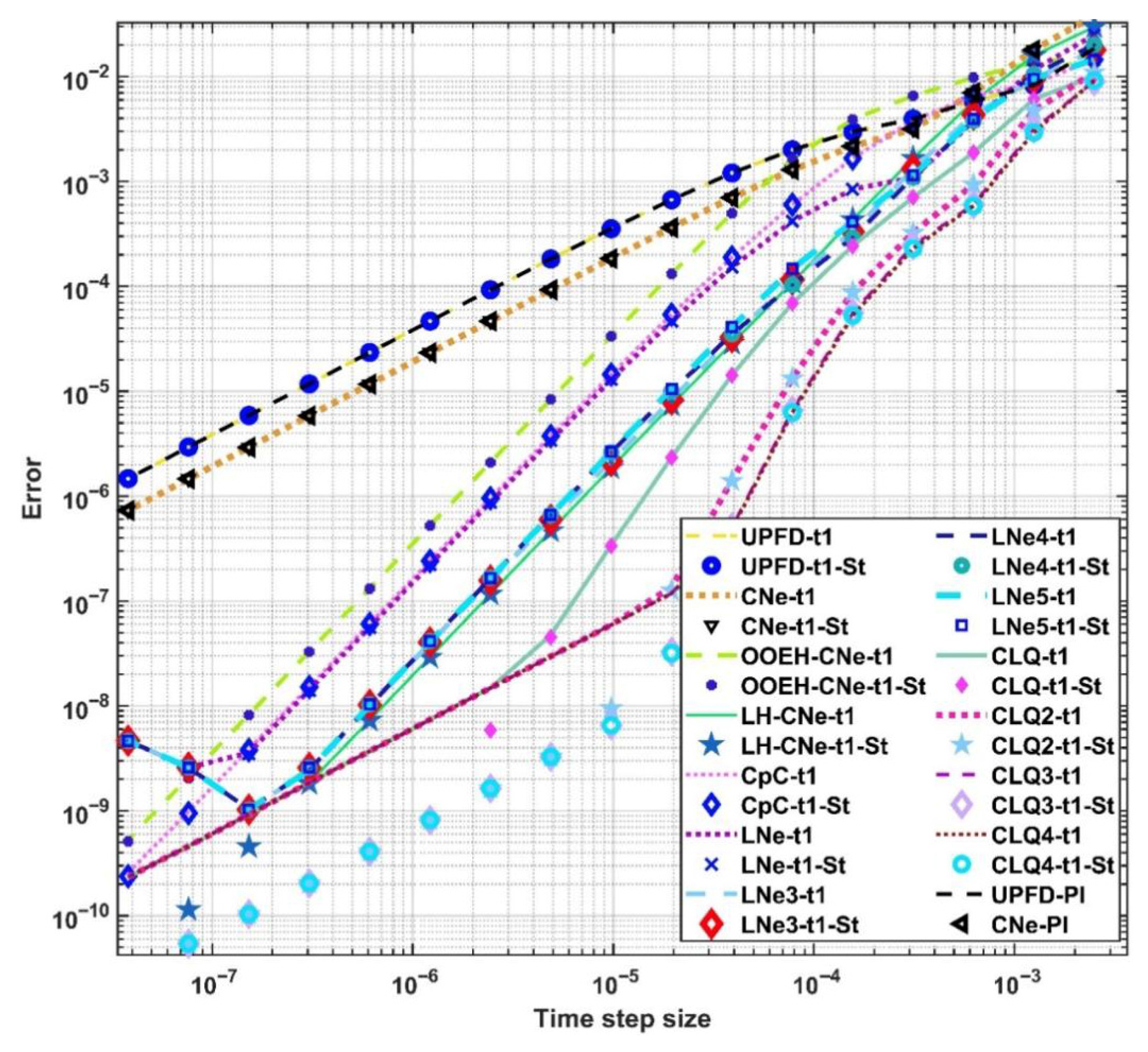
In order to verify the algorithm combinations, we set P = 18, and plot the errors as a function of the time-step size. However, instead of displaying the $5\times 13=65$ curves for each case study, we select those using the PI reaction-term treatment in Case Study 1 with all the diffusion-solvers in Figure 2, while choosing three different diffusion-solvers combined with all the reaction-term treatments in Figure 3. Very similarly, for Case Study 2, we present the error curves for all diffusion-solvers using the t2 reaction-treatment, and then the five reaction-treatments combined with only three diffusion-solvers, in Figure 4 and Figure 5, respectively.

The numerical order of convergence has been calculated for the two cases displayed in Figure 2 and Figure 4 and presented in

Table 2. The theoretical order for the diffusion equation and numerical orders of the methods for the PI treatment in Case Study 1.

Num. Method (Theor. Order)	Time-Step Size	Error (L∞)	NO
UPFD (1)	h17 = 9.9 × 10−6	5.0 × 10−4	0.98
	h18 = 4.9 × 10−6	2.5 × 10−4
CNe (1)	h17 = 9.9 × 10−6	2.5 × 10−4	1.0
	h18 = 4.9 × 10−6	1.3 × 10−4
OOEH-CNe (2)	h17 = 9.9 × 10−6	7.8 × 10−6	2.3
	h18 = 4.9 × 10−6	1.6 × 10−6
LH-CNe (2)	h17 = 9.9 × 10−6	1.7 × 10−6	2.8
	h18 = 4.9 × 10−6	2.4 × 10−7
CpC (2)	h17 = 9.9 × 10−6	4.7 × 10−6	2.3
	h18 = 4.9 × 10−6	9.3 × 10−7
LNe (2)	h17 = 9.9 × 10−6	5.7 × 10−6	2.2
	h18 = 4.9 × 10−6	1.2 × 10−6
LNe3 (2)	h14 = 1.5 × 10−4	5.4 × 10−5	2.7
	h15 = 7.9 × 10−5	8.1 × 10−6
LNe4 (2)	h13 = 3.1 × 10−4	9.5 × 10−5	3.2
	h14 = 1.5 × 10−4	1.1 × 10−5
LNe5 (2)	h12 = 6.3 × 10−4	3.2 × 10−4	3.4
	h13 = 3.1 × 10−4	3.1 × 10−5
CLQ (3)	h14 = 1.5 × 10−4	4.1 × 10−5	2.5
	h15 = 7.9 × 10−5	7.4 × 10−6
CLQ2 (4)	h12 = 6.3 × 10−4	3.6 × 10−4	2.9
	h13 = 3.1 × 10−4	4.8 × 10−5
CLQ3 (4)	h11 = 1.2 × 10−3	9.7 × 10−4	3.0
	h12 = 6.3 × 10−4	1.1 × 10−4
CLQ4 (4)	h11 = 1.2 × 10−3	4.5 × 10−4	2.8
	h12 = 6.3 × 10−4	6.1 × 10−5

and

Table 3. The theoretical order for the diffusion equation and numerical orders of the methods for the t2 treatment in Case Study 2.

Num. Method (Theor. Order)	Time-Step Size	Error (L∞)	NO
UPFD (1)	h17 = 1.4 × 10−6	5.8 × 10−3	0.91
	h18 = 7.2 × 10−7	3.1 × 10−3
CNe (1)	h17 = 1.4 × 10−6	3.3 × 10−3	0.99
	h18 = 7.2 × 10−7	1.7 × 10−3
OOEH-CNe (2)	h17 = 1.4 × 10−6	8.6 × 10−4	1.9
	h18 = 7.2 × 10−7	2.2 × 10−4
LH-CNe (2)	h17 = 1.4 × 10−6	2.2 × 10−4	2
	h18 = 7.2 × 10−7	5.5 × 10−5
CpC (2)	h17 = 1.4 × 10−6	4.4 × 10−4	1.8
	h18 = 7.2 × 10−7	1.2 × 10−4
LNe (2)	h17 = 1.4 × 10−6	5.2 × 10−4	1.8
	h18 = 7.2 × 10−7	1.4 × 10−4
LNe3 (2)	h17 = 1.4 × 10−6	9.5 × 10−5	2.6
	h18 = 7.2 × 10−7	1.5 × 10−5
LNe4 (2)	h17 = 1.4 × 10−6	1.9 × 10−5	3.3
	h18 = 7.2 × 10−7	1.9 × 10−6
LNe5 (2)	h17 = 1.4 × 10−6	4.6 × 10−6	3.7
	h18 = 7.2 × 10−7	7.5 × 10−7
CLQ (3)	h17 = 1.4 × 10−6	6.8 × 10−5	2.6
	h18 = 7.2 × 10−7	1.1 × 10−5
CLQ2 (4)	h16 = 2.8 × 10−6	8.3 × 10−5	3.2
	h17 = 1.4 × 10−6	8.9 × 10−6
CLQ3 (4)	h15 = 5.7 × 10−6	1.7 × 10−5	3.6
	h16 = 2.8 × 10−6	2.5 × 10−6
CLQ4 (4)	h15 = 5.7 × 10−6	5.5 × 10−6	3.6
	h16 = 2.8 × 10−6	2.5 × 10−6

, respectively. For this, we chose two values of the errors belonging to two subsequent time-step sizes using the formula

$$Error\sim h^{NO}\Rightarrow NO={\displaystyle \frac{\mathit{log}\frac{\mathrm{Error}\left(L_{\infty }\right)\left(h_k\right)}{\mathrm{Error}\left(L_{\infty }\right)\left(h_{k+1}\right)}}{\mathit{log}\left(h_k/h_{k+1}\right)}}={\displaystyle \frac{\mathit{log}\frac{\mathrm{Error}\left(L_{\infty }\right)\left(h_k\right)}{\mathrm{Error}\left(L_{\infty }\right)\left(h_{k+1}\right)}}{\mathit{log}2}}.$$

The values of the first time-step size $h_k$ and the subsequent time-step size $h_{k+1}=h_k/2$ have been chosen in such a way as to obtain the maximal value for NO. The exception is the first (and largest) time-step size, where the observed significant drop of the error does not reflect the order of the methods (see the top-right corner of Figure 2 and Figure 4), and hence this k = 1 case is not sampled. One can observe that the numerical orders are not far from the theoretical orders which were calculated for the pure diffusion equation.

Very similar error curves have been obtained for other values of the parameters β, $t^{\mathrm{fin}}$, Δx and for the remaining algorithm combinations as well. The methods converge smoothly, and unstable behavior or unphysical oscillations are not produced. The only exception is treatment 3, which does not converge; therefore, we omit it from further investigations. The remaining four reaction-treatments are organized with halved time steps by Strang-splitting as well. In this way, 12 treatments are constructed and tested with the 13 diffusion-solvers, i.e., 12 × 13 = 156 algorithm combinations are tested. 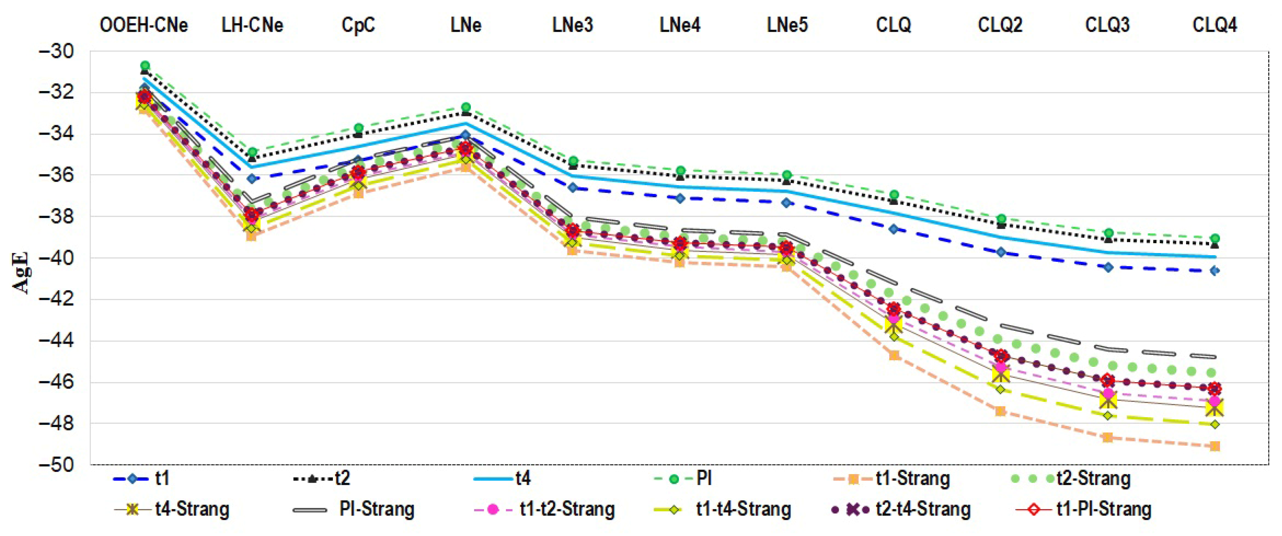Considering that we have two test problems and P = 13 different time-step sizes, we performed 4056 runs with error calculations. The AgE values are tabulated in

Table 4. The AgE errors for different treatments of the diffusion and the nonlinear term in Case Study 1.

	Treatment of the Nonlinear Term
Method	t1	t2	t4	PI	t1-Strang	t2-Strang	t4-Strang	PI-Strang	t1-t2-Strang	t1-t4-Strang	t2-t4-Strang	t1-PI-Strang
UPFD	−41.98	−41.99	−41.98	−41.99	−42.00	−42.00	−42.00	−42.00	−42.00	−41.996	−41.99	−41.99
CNe	−45.99	−46.00	−45.97	−45.98	−45.99	−46.00	−45.99	−45.99	−46.00	−45.99	−45.99	−45.99
OOEH-CNe	−60.50	−59.73	−59.47	−58.46	−63.41	−61.58	−61.64	−60.42	−63.41	−62.41	−61.61	−61.62
LH-CNe	−60.15	−59.37	−58.93	−58.55	−65.26	−62.96	−63.06	−61.58	−63.95	−64.01	−63.03	−63.02
CpC	−61.85	−60.91	−60.60	−59.38	−65.63	−63.21	−63.31	−61.75	−64.24	−64.29	−63.25	−63.25
LNe	−61.42	−60.59	−60.30	−59.13	−65.05	−62.76	−62.82	−61.39	−62.82	−63.81	−62.82	−62.82
LNe3	−61.74	−60.85	−60.55	−59.33	−65.53	−64.16	−63.22	−61.68	−64.16	−64.21	−63.18	−63.19
LNe4	−61.76	−60.87	−60.57	−59.34	−65.56	−63.16	−63.24	−62.36	−64.18	−64.23	−63.20	−63.21
LNe5	−61.77	−60.88	−60.57	−59.35	−65.57	−63.17	−63.25	−61.70	−64.19	−64.24	−63.21	−63.22
CLQ	−62.23	−61.28	−60.98	−59.60	−65.22	−64.03	−64.15	−62.24	−63.92	−64.03	−64.03	−62.99
CLQ2	−62.26	−61.29	−60.99	−59.61	−67.18	−63.95	−64.18	−62.26	−65.27	−65.42	−64.07	−64.07
CLQ3	−62.26	−61.29	−60.99	−59.61	−67.18	−63.96	−64.18	−62.26	−65.27	−65.42	−64.07	−64.07
CLQ4	−62.26	−61.29	−60.99	−59.61	−67.18	−63.96	−64.18	−62.26	−65.27	−65.42	−64.07	−64.07

and

Table 5. The AgE errors for different treatments of the diffusion and the nonlinear term in Case Study 2.

Methods	t1	t2	t4	PI	t1-Strang	t2-Strang	t4-Strang	PI-Strang	t1-t2-Strang	t1-t4-Strang	t2-t4-Strang	t1-PI-Strang
UPFD	−22.37	−22.58	−22.65	−22.49	−22.8	−22.73	−22.76	−22.69	−22.76	−22.78	−22.74	−22.74
CNe	−24.97	−24.67	−24.82	−24.54	−25.07	−24.93	−25	−24.86	−25.01	−25.04	−24.7	−24.99
OOEH-CNe	−31.79	−30.91	−31.34	−30.66	−32.82	−31.97	−32.38	−31.75	−32.32	−32.58	−32.17	−32.18
LH-CNe	−36.16	−35.15	−35.62	−34.85	−38.93	−37.60	−38.26	−37.29	−38.12	−38.55	−37.90	−37.91
CpC	−35.26	−34.00	−34.60	−33.68	−36.89	−35.54	−36.19	−35.22	−36.07	−36.49	−35.83	−35.84
LNe	−34.05	−32.94	−33.48	−32.66	−35.60	−34.41	−34.99	−34.12	−34.88	−35.26	−34.67	−34.68
LNe3	−36.58	−35.52	−36.03	−35.24	−39.60	−38.35	−39.00	−38.03	−38.84	−39.26	−38.64	−38.65
LNe4	−37.09	−36.03	−36.54	−35.75	−40.21	−38.97	−39.61	−38.64	−39.46	−39.87	−39.26	−39.27
LNe5	−37.30	−36.24	−36.75	−35.96	−40.44	−39.19	−39.84	−38.86	−39.68	−40.10	−39.48	−39.49
CLQ	−38.57	−37.22	−37.85	−36.90	−44.69	−41.80	−43.16	−41.18	−42.89	−43.81	−42.43	−42.44
CLQ2	−39.71	−38.36	−38.99	−38.05	−47.38	−43.97	−45.59	−43.26	−45.27	−46.35	−44.70	−44.71
CLQ3	−40.42	−39.08	−39.70	−38.77	−48.68	−45.16	−46.84	−44.43	−46.50	−47.62	−45.92	−45.93
CLQ4	−40.65	−39.31	−39.93	−39.00	−49.08	−45.52	−47.23	−44.79	−46.89	−48.02	−46.30	−46.31

and visualized in Figure 6 and Figure 7 for Case Study 1 and 2, respectively. We note that the errors of the different treatments are sometimes very close to each other, so the difference between them is only in the third or fourth decimals.

Based on Figure 6 and Figure 7 and Table 4 and Table 5, and further results we do not present here for brevity, we intend to remove those combinations which were clearly outperformed by others. First, we can conclude that the t1 treatment with Strang-splitting is the most accurate, while the PI treatment is the least accurate. Strang-splitting yields a significant increase in accuracy, typically for the higher-order schemes, e.g., for the CLQ3 and CLQ4 schemes, which are more accurate for the diffusion equation. For the first-order UPFD and CNe solvers, the difference in accuracy between the reaction-treatments is very small. The mixing of the treatments by Strang-splitting does not yield any substantial improvement. Moreover, they require more effort to code, so we exclude them from future investigations. However, when we select the methods for further investigation, including running time tests, we have to be careful: not only the accuracy but also the speed has to be considered. The multi-stage diffusion-solvers are more accurate, but slower as well, and thus we keep both low- and high-order solvers. On the other hand, the formula of the t1–t4 treatments contains the calculation of the exponential function in each time step for each cell, e.g., $e^{-u_i^{\mathrm{diff}}\beta t}$, while the PI treatment contains cheaper operations. Furthermore, Strang-splitting also consumes time. Therefore, although we select mainly the t1 and t1-Strang treatments, we keep the PI treatment combined with the simplest UPFD and CNe solver, hoping that the speed gain can dominate the loss in the accuracy, at least in some cases. To summarize, we decided to keep the following 28 combinations:

UPFD-PI	OOEH-CNe-t1-Strang	LNe3-t1	CLQ-t1-Strang
UPFD-t1	LH-CNe-t1	LNe3-t1-Strang	CLQ2-t1
UPFD-t1-Strang	LH-CNe-t1-Strang	LNe4-t1	CLQ2-t1-Strang
CNe-PI	CpC-t1	LNe4-t1-Strang	CLQ3-t1
CNe-t1	CpC-t1-Strang	LNe5-t1	CLQ3-t1-Strang
CNe-t1-Strang	LNe-t1	LNe5-t1-Strang	CLQ4-t1
OOEH-CNe-t1	LNe-t1-Strang	CLQ-t1	CLQ4-t1-Strang

6. Testing the Performance with Running Time Measurements in 2D

The capacity-resistivity model, introduced in Section 2, will be used for the simulations in two spatial dimensions here and in the next section. This means that the ODE system (8), supplemented with the Huxley reaction term, is solved by the selected 28 algorithm combinations. The CFL limit and the stiffness ratio can be adjusted by generating random values for the C and R quantities following a log-uniform distribution:

$$C_i={10}^{(a_C-b_C\cdot rand)}, R_{x,i}={10}^{(a_{Rx}-b_{Rx}\cdot rand)}, R_{y,i}={10}^{(a_{Ry}-b_{Ry}\cdot rand)}.$$

(30)

Here, rand are random numbers, uniformly distributed in the unit interval by MATLAB R2021b. We assume that if our methods work in the case of random systems, they will work in other cases as well. We construct two completely different systems and via running-time measurements, try to obtain the methods with the best performance. In all 2D cases, the reference solutions are calculated by the MATLAB built-in ode15 solver using a very strict absolute and relative error tolerance. The tic-toc command of MATLAB is utilized to measure the running times, which are good approximations of the CPU times if no other tasks are given to the computer, which has a 13th Gen Intel Core i7-13700 CPU and 64GB RAM. We tried to minimize the running-time measurement errors appearing as random fluctuations by repeating the calculations more times subsequently, and then taking the average of the measured running times.

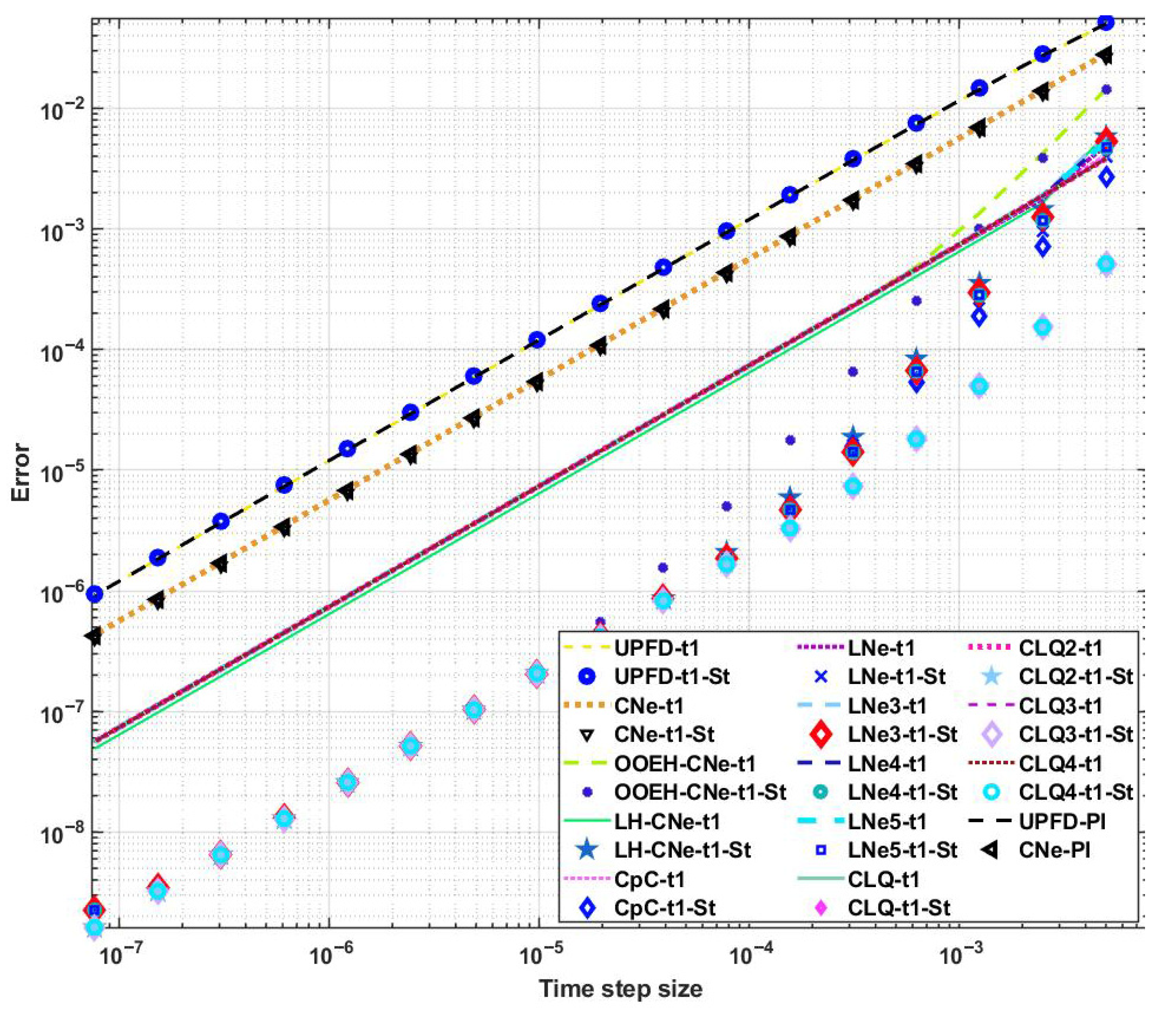
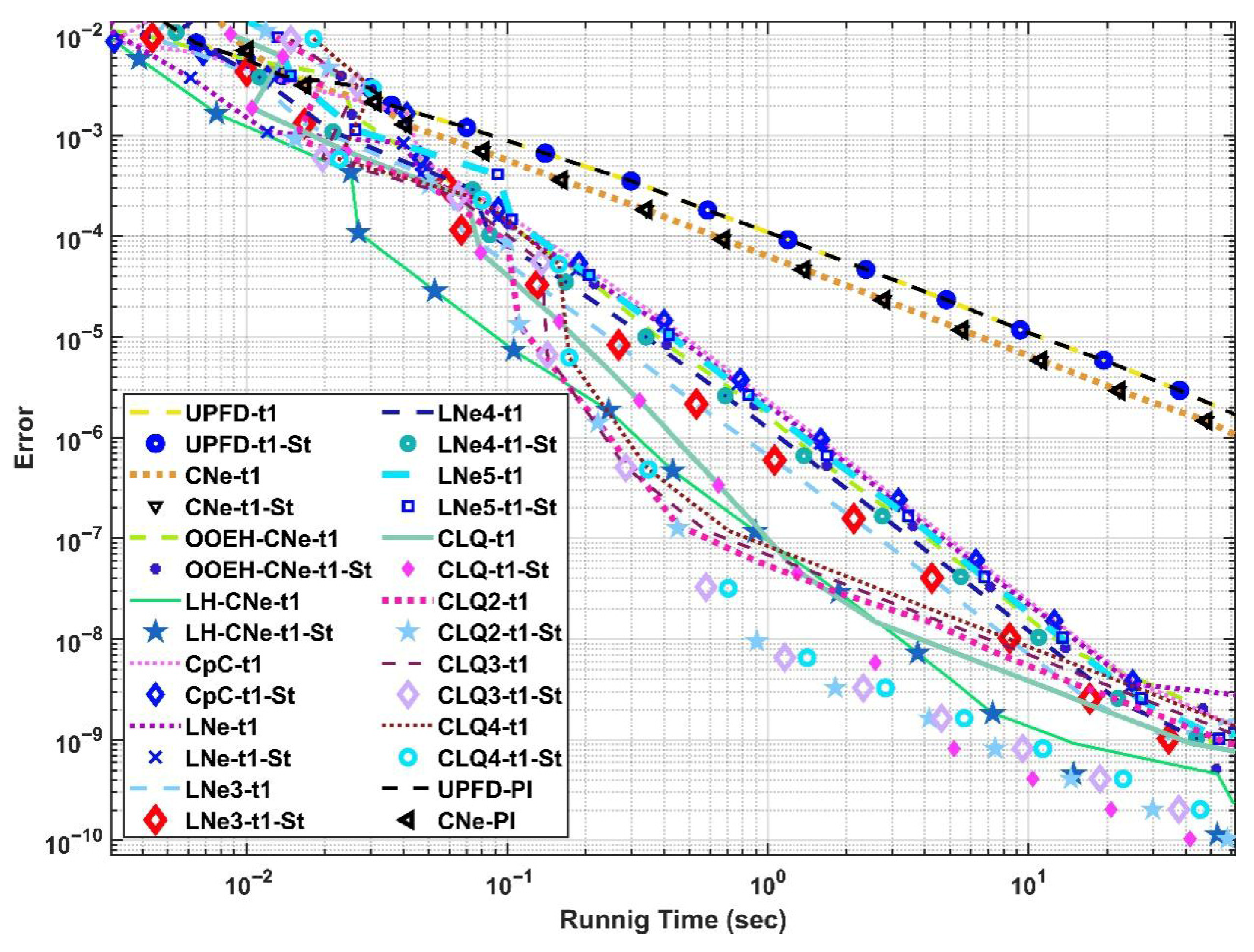
Case Study 3: A moderately stiff system with stronger nonlinearity

The mesh size and final time used are $N_x=51,\hspace{0.33em}{N}_y=60,\hspace{0.33em}{t}^{\mathrm{fin}}=0.02,$ while $\beta =11$, and $a_C=1,\hspace{0.33em}{b}_C=2,\hspace{0.33em}{a}_{Rx}=1,\hspace{0.33em}{b}_{Rx}=2,\hspace{0.33em}{a}_{Rz}=1,\hspace{0.33em}{b}_{Rz}=2$. These parameters yield $SR=1.9\cdot 10^5$ and $h_{MAX}^{FTCS}=8.5\cdot 10^{-3}$, which means that the system is mildly stiff. The initial concentrations are random numbers: $u_i^0=rand$. The errors as a function of the time-step size and running times are presented in Figure 8 and Figure 9, respectively.

Case Study 4: A stiff system with weaker nonlinearity

The size of the system is $N_x=51,\hspace{0.33em}{N}_y=60,$ the final time is $\hspace{0.33em}{t}^{fin}=0.01,$ the coefficient of the reaction term is $\beta =2.9$, while the exponents are $a_C=3, b_C=6, a_{Rx}=1, b_{Rx}=2, a_{Ry}=2, b_{Ry}=4$. The problem we obtained using these parameters is characterized by the $SR=2.68\cdot 10^9$ and $h_{MAX}^{FTCS}=2.1\cdot 10^{-5}$ numbers, and hence the system is rather stiff. The initial concentration function is smooth: $u_i^0={\displaystyle \frac{1}{\sqrt{1+i}}}+0.001$. The errors as a function of the time-step size and running times are presented in Figure 10 and Figure 11, respectively.

Using the results accumulated up to this point, we further reduce the number of methods, and we keep only the top nine of them. These are the OOEH-CNe-t1-Strang, LH-CNe-t1, LH-CNe-t1-Strang, CpC-t1-Strang, and LNe-t1-Strang, as well as four higher-order combinations: the CLQ-CLQ4 series with the t1 treatment and Strang-splitting.

7. Parameter-Sweep for Further Testing of the Performance of the Top 9 Methods

Case Study 5: Errors as a function of the β parameter, non-stiff case

The following series is used for the values of the nonlinear coefficient: $\beta \in \left\{0,\hspace{0.33em}0.25, 1,\hspace{0.33em}2,\hspace{0.33em}5,\hspace{0.33em}10,\hspace{0.33em}15,\hspace{0.33em}20,\hspace{0.33em}30,\hspace{0.33em}50\right\}$. To construct a system with the lowest possible stiffness ratio, all a and b exponents are set to zero, i.e., $C=1, R_x=R_y=1$ for all cells. The system size is set to $N_x=21$ and $N_y=12$, and the final time is $t^{fin}=2.1$. The initial concentration function is given by $u_i^0={\displaystyle \frac{2}{i+2}}+0.2 rand$. 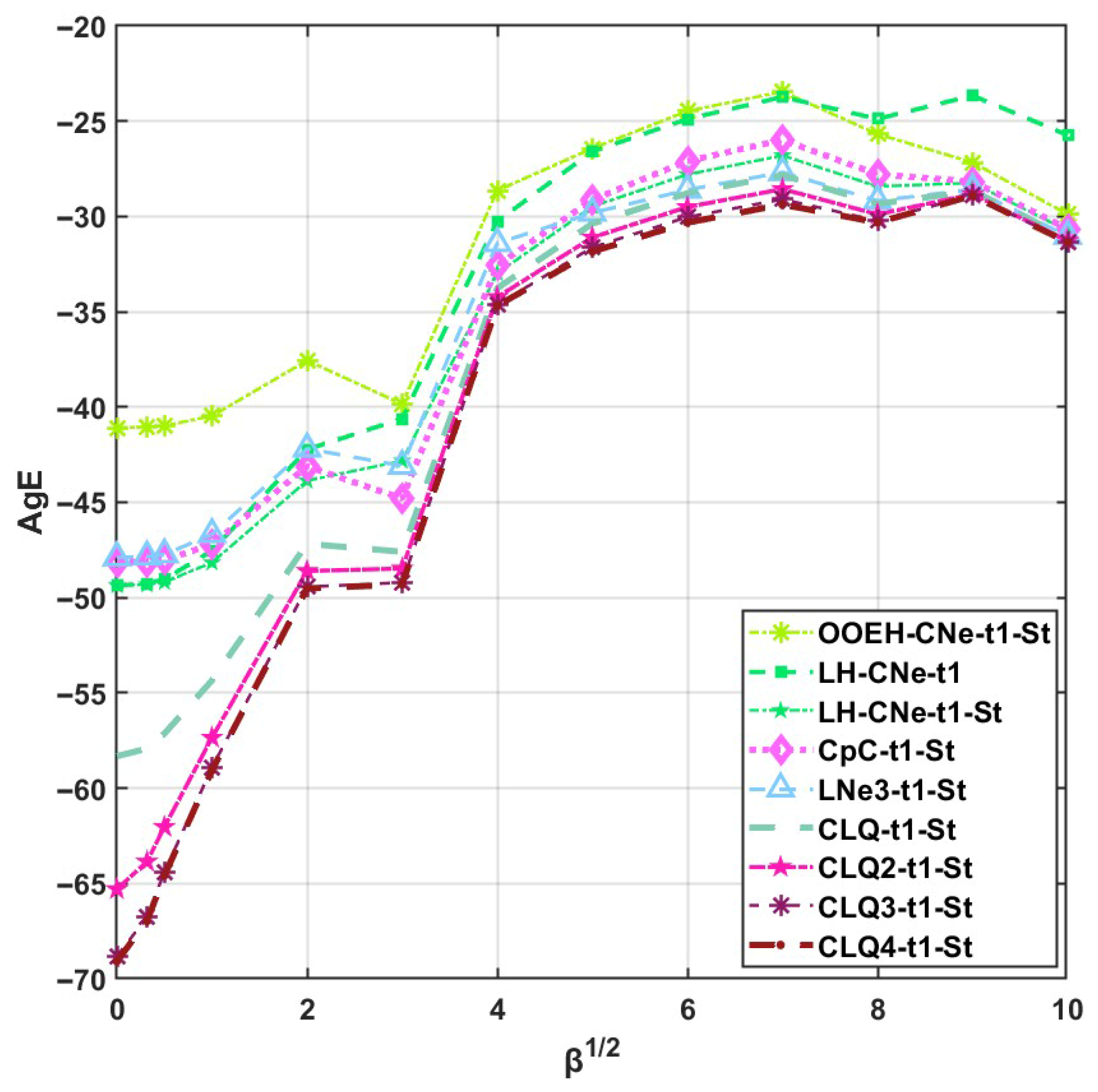Figure 12 shows the AgE errors as a function of the square root of the β coefficient. One can observe that the errors increase when the level of nonlinearity is increasing until $\beta \approx 5$. If β surpasses this region, the solution function is extremely close to 1; therefore, the errors become smaller and smaller again. In this region, the diffusion-solver has no significance, while the Strang-splitting yields a slight but noticeable advantage.

Case Study 6: Errors as a function of the β parameter, stiff case

The following series is used for the values of the nonlinear coefficient: $\beta \in \left\{0,\hspace{0.33em}0.1, 0.25, 1,\hspace{0.33em}4,\hspace{0.33em}9, 16, 25,\hspace{0.33em}36,\hspace{0.33em}64,\hspace{0.33em}81,\hspace{0.33em}100\right\}$. The a and b exponents are larger: $a_C=3, b_C=6, a_{Rx}=1, b_{Rx}=2, a_{Ry}=2, b_{Ry}=4$. The system size is set to $N_x=15$ and $N_y=20$, and the final time is $t^{fin}=0.2$. The initial concentration function is given by $u_i^0={\displaystyle \frac{1}{i+2}}+0.4 rand$. Figure 13 shows the AgE errors as a function of $\sqrt{\beta }$. One can see that the accuracy of the methods deteriorates when the β parameter is increasing, but the higher-order diffusion-solvers lose their advantage at a much slower rate than for a non-stiff system.

Case Study 7: Errors as a function of the CFL limit

A series of test problems with a decreasing CFL limit and increasing stiffness ratio has been set up by gradually increasing the a and b exponents in (30), as

Table 6. Data of the 10 random systems produced with a decreasing CFL limit (increasing stiffness ratio).

Number	aC	bC	aRx	bRx	aRy	bRy	${\mathit{h}}_{\mathit{M}\mathit{A}\mathit{X}}^{\mathit{R}\mathit{K}1}$	SR
1	0	0	0	0	0	0	0.25	5.04 × 102
2	−1	1	0	0	0	0	0.04	7.3 × 103
3	−1	1	−1	1	0	0	0.015	1.8 × 104
4	−1	1	−1	1	−1	1	6.5 × 10−3	5.0 × 104
5	−2	2	−1	1	−1	1	7.9 × 10−4	1.9 × 106
6	−2	2	−2	2	−1	1	2.5 × 10−4	5.3 × 106
7	−2	2	−2	2	−2	2	1.0 × 10−4	1.8 × 107
8	−3	3	−2	2	−2	2	2.5 × 10−5	5.9 × 108
9	−3	3	−3	3	−2	2	4.7 × 10−6	3.5 × 109
10	−3	3	−3	3	−3	−3	1.4 × 10−6	9.1 × 109

shows. All other parameters are kept fixed, such as $\beta =4.3$, $N_x=25$ and $N_y=22$, and $t^{fin}=0.2$. The initial values were generated only once for all the cases using the formula $u_i^0={\displaystyle \frac{3}{i+5}}+0.5 rand$. P = 15 different time-step sizes have been used in the definitions (28) and (29) of the aggregated error.

The AgE errors for different CFL limits are presented in Figure 14 and

Table 7. The AgE errors for a decreasing CFL limit (increasing stiffness) in Case Study 7. The serial numbers in the first row are explained in Table 6.

Method	1	2	3	4	5	6	7	8	9	10
OOEH-CNe-t1-St	−63.06	−59.88	−58.34	−56.07	−50.93	−43.27	−39.04	−34.32	−28.19	−23.69
LH-CNe-t1	−57.18	−55.33	−53.65	−53.94	−50.08	−45.07	−41.22	−35.71	−30.75	−28.20
LH-CNe-t1-St	−63.15	−60.98	−60.63	−58.15	−53.67	−47.46	−42.81	−37.42	−31.63	−28.74
CpC-t1-St	−63.10	−60.97	−60.71	−58.50	−53.15	−47.15	−42.97	−37.34	−32.73	−28.47
LNe3-t1-St	−63.08	−60.93	−61.03	−58.59	−53.58	−48.50	−43.98	−39.25	−32.92	−30.51
CLQ-t1-St	−63.09	−61.16	−61.69	−59.87	−55.57	−51.77	−48.28	−40.72	−38.08	−33.79
CLQ2-t1-St	−63.09	−61.15	−61.93	−60.45	−55.99	−52.89	−49.33	−43.08	−39.36	−35.83
CLQ3-t1-St	−63.10	−61.15	−62.04	−60.74	−56.19	−53.68	−50.39	−44.55	−40.29	−37.40
CLQ4-t1-St	−63.11	−61.16	−62.04	−60.81	−56.18	−53.87	−50.43	−45.51	−40.44	−38.16

. As was expected, the accuracy of the methods deteriorates with a decreasing CFL limit and increasing stiffness ratio. The high-order CLQ family has a large relative advantage for a small CFL limit. The error of the OOEH scheme increases faster than those of the other schemes with a decreasing CFL limit and exceeds the error of the LH-CNe without Strang-splitting.

8. Discussion and Summary

The numerical solution of a special form of the nonlinear Huxley equation is examined, for which the true solution remains in the unit interval. We constructed numerous algorithm combinations with operator-splitting and showed that they preserve this property for arbitrary spatial mesh, the time-step size, and values of the nonlinear coefficient β. The numerical experiments confirmed these results and helped us to gradually tighten the large set of the examined methods to find the best choices for different circumstances. We can propose the LH-CNe diffusion-solver combined with t1 treatments and Strang-splitting if any of the following conditions are fulfilled:

• Speed is more important than the accuracy of the result.
• The CFL limit is moderate or the stiffness is not high.
• The nonlinear parameter β is large: larger than 1 for an equidistant mesh or larger than 5 for a stiff case.

However, if high accuracy is required in a stiff case, the CLQ family combined with t1 treatments and Strang-splitting is the best choice. Furthermore, if the nonlinearity is very low, Strang-splitting is redundant, but in all other cases, it is worth coding. If one has a physical system with a complicated geometry, the odd–even hopscotch structure may be hard to construct. In those cases, the CpC-t1-Strang solver can be recommended if high speed is required, since the diffusion-solver CpC contains only two stages, and it usually yields an acceptable accuracy.