Assessment of Efficiency of Last-Mile Delivery Zones: A Novel IRN OWCM–IRN AROMAN Model

Abstract

The importance of managing goods delivery in urban areas has reached its peak in recent years, driven by the constant and rapid growth of online commerce. Under such conditions, where smaller quantities of goods are ordered, yet the number of shipments continues to rise, the question of last-mile delivery (LMD) efficiency becomes increasingly relevant. This paper addresses the issue of last-mile delivery zone efficiency through the application of a new methodological approach. First, the concept of measuring last-mile delivery productivity is defined using a specific example from an urban environment. Next, Key Performance Indicators (KPIs) are established to enable a proper assessment of urban zone efficiency in line with the LMD concept. The main contribution of this study is the development of the IRN OWCM (Interval Rough Number Opinion Weight Criteria Method), which is used to calculate the weights of the criteria. To assess suitable delivery zones in terms of efficiency based on the defined KPIs, the previously developed IRN OWCM method is integrated with IRN AROMAN (Alternative Ranking Order Method Accounting for Two-Step Normalization). The results identify delivery zones that are suitable in terms of meeting standardized user needs. The developed model demonstrated stability through additional verification tests and can be adequately applied in cases when it is needed to minimize subjectivity and uncertainties.

1. Introduction

The rapid growth of e-commerce in recent decades has presented numerous challenges for postal operators, including increased parcel volumes, limited infrastructure, parking constraints, and failed deliveries. Consequently, the delivery of small and lightweight parcels (weighing up to 31.5 kg) has become a rapidly expanding sector. This segment increasingly relies on advanced logistics networks and sophisticated parcel tracking systems to meet rising demand [1].

As demands for shipments grow exponentially, the negative impacts on transportation systems are receiving increasing attention [2]. This raises questions about sustainability. Sustainable business refers to managing a business entity in a way that balances economic goals with environmental protection and social responsibility. The postal sector plays a significant role in sustainability, as the management of its internal processes directly affects CO₂ emissions and the overall ecological footprint. Optimizing delivery areas in cities enables reduced fuel consumption and fewer kilometers travelled, as well as better vehicle utilization. Efficient planning and balancing of delivery areas contribute to a more environmentally responsible postal service provision. By implementing sustainable delivery areas, postal operators not only reduce costs but also strengthen their image as socially responsible companies. Consequently, proper organization of delivery areas is gaining prominence to achieve optimal solutions in the functioning of postal operators.

One of the criteria often used to assess successful business operations in the postal sector is productivity. Specifically, productivity is often broken down to the level of individual workers, where their productivity is evaluated to determine if they are efficient or not. Thus, productivity reflects the workload of a particular worker. If productivity levels are not taken into account, this can result in high turnover rates among workers in observed positions. This, in turn, leads to a certain period of “ramp-up” for new workers to reach the performance levels of their predecessors, which further costs the operator. Assessing the productivity of delivery men/couriers as the final element in last-mile delivery is particularly challenging, as the outcome of their work is not a one-dimensional output. Considering the array of activities assigned by the employer, including the crucial element of empathy towards the customer (achieving customer satisfaction with the service), it is questionable whether all necessary elements for successful parcel delivery can be encompassed within the concept of productivity. However, in most cases, productivity is the dimension that receives the most attention, thus neglecting other elements from a sustainability perspective.

To determine the workload of a specific region in cities serviced by a delivery provider, we attempted to rank them through real data made available to us by a private postal operator (from which we defined KPIs) using the IRN MCDM (Multi-Criteria Decision-Making) model. The reference point taken was the 100% productivity of a public postal operator in a hypothetical delivery area.

The analysis is focused on a medium-sized urban area that is experiencing growth in delivery volume yet does not represent an overly complex agglomeration. This choice of context enabled a realistic, yet methodologically manageable, analysis of the problem of uneven workload distribution across delivery areas.

1.1. Motivation for Research

In urban areas, unevenly distributed work tasks across district boundaries often lead to an imbalanced workload for delivery personnel, which directly affects their productivity, work efficiency, and job satisfaction. In the context of sustainable business practices, fairly allocated delivery areas and realistic workload assessments become key factors in reducing the negative environmental impact and improving the social aspects of work. Optimizing delivery areas not only contributes to reducing the distance traveled and fuel consumption but also enables better utilization of vehicles and a more balanced distribution of workload among delivery workers. One common indicator of business success in the postal sector is employee productivity, which is often measured without considering the complexity and differences between zones. Such an approach can be unfair and may lead to a high risk of turnover, employee dissatisfaction, and additional costs due to the need for training new workers. There is a need for further empirical research that would incorporate direct economic indicators linking courier turnover with overall operational costs, given that currently available financial reports from the Serbian Business Registers Agency do not contain such data, and among operators, this information is typically treated as confidential.

The motivation for this research stems from the need to define key performance indicators (KPIs) based on real operational data, which, through more precise and fairer productivity evaluation, allow the identification of delivery zones at risk of overload and enable decision-making based on objective criteria.

1.2. Aims of Research

The aim of this research is to identify and objectively assess delivery areas in urban environments based on real operational data from a postal operator, focusing on their workload and work sustainability. The key objectives of the study are as follows:

-

Fairer evaluation of delivery personnel productivity: Develop a model that enables a more realistic and equitable assessment of delivery workers’ productivity, specifically through a more appropriate valuation of the distance traveled;

-

Determination of delivery zone workload levels: Using key performance indicators (KPIs) to identify zones that are overloaded, balanced, or underutilized, with the goal of better organizing delivery areas;

-

Contribution to more sustainable and efficient delivery planning in urban environments: Provide guidelines to postal operators for optimizing district workload distribution and reducing negative environmental impacts, while increasing operational efficiency and employee satisfaction.

1.3. Scientific and Professional Contributions

The contributions identified in this research are evident in both scientific and professional domains. The scientific contribution lies in the extension of the OWCM method through the incorporation of interval rough numbers (IRN), resulting in a completely new approach that allows for a more accurate determination of criteria weights by incorporating expert preferences. By applying this approach, experts can express subjective preferences based on objectively available quantitative data. Subsequent scientific and methodological processing then yields more precise values for the criteria weights.

In addition, the developed IRN OWCM model has the following advantages: it allows experts to use a modified well-known linguistic Likert scale for the assessment of potential variants. Very often, it is difficult for experts to use a complicated methodological framework to access alternatives, so we have tried to solve this problem by proposing the IRN OWCM methodology. Furthermore, the model can use both types of data, quantitative or qualitative, especially with the note that for some of the MCDM cases, experts can make assessments in the absence of data based on their knowledge and skills.

From a professional standpoint, the contributions are reflected in the application of the developed approach, combined with the IRN AROMAN method, to rank delivery areas according to defined KPIs and compare them with a reference model of the ideal area for a public postal operator.

2. Literature Review

This section presents a literature review based on three key aspects: productivity, modern solutions in last-mile delivery management, and the application of MCDM methods for solving problems in the subject area, including the selection of methods for ranking delivery areas.

2.1. Literature Review on Productivity

Productivity represents the ratio of outputs to inputs in a specific production situation [3]. The basic components of productivity measurement are labor productivity and capital productivity [4]. From a microeconomic perspective, productivity aims to reduce costs, provide the possibility of lower price formation, and reduce working hours. At the macro level, it enables an increase in the standard of living and a more convenient supply of goods and services, accompanied by an increase in real incomes. High productivity should ensure the well-being of those who possess it [5]. Why do companies differ so much in their ability to convert inputs into outputs [6]? Factors influencing productivity include technological innovations, economies of scale, and employee training (motivation, engagement) [7]. Long-term productivity growth is primarily based on innovations and technological progress [8]. Productivity based on manual labor is limited by human capacity, so expecting significant productivity growth primarily from labor-intensive activities is unrealistic. Productivity is often used as a measure of competitiveness between companies, individuals, or facilities within companies [9]. Productivity can also be a measure of the engineering efficiency of a specific process or transformation activity [10]. Productivity represents the ability to produce goods and services compared with the resources required for their production [11]. Productivity data are applied to investigate the impact of market and labor regulation on economic performance [12]. Such data allow analysts to determine the capacity utilization of the observed system. Production capacity is used to assess demand and inflationary pressure [13]. The difference in productivity can be a cause of long-term differences in sales growth. Industry leaders in services are companies that focus on fast and smooth flow in their operations and therefore demonstrate better results compared with the competition. A higher flow of goods and information within processes leads to greater process productivity [14]. Therefore, the oscillation that occurs in this case is associated with fluctuations in the level of quality, quantity, and timing. The superior performance of certain service companies indicates that their productivity is at a higher level than that of the competition. Schmenner finds a way to determine this by understanding the productivity of service operations and provides assistance in explaining how some leading service companies manage to maintain their leading positions for decades [15].

Demand also affects productivity, ranging from cases where it is low and system performance is compromised to situations where positive effects on productivity occur when things change course. Time, as a non-renewable resource, lies at the core of productivity: how much can we accomplish with the resources we have? Understanding how the number of working hours defines productivity is the starting point for the demand for labor [16]. There is a dilemma between shorter and longer working hours. On one hand, longer working hours lead to better utilization of capital goods, but only if the worker is exposed to fixed costs and fixed non-productive time during working hours [17]. On the other hand, the argument favors the danger of worker fatigue that occurs after a while, subsequently leading to a decrease in productivity [18] and even to worker injury. Numerous studies indicate that overtime work for extended periods is harmful to health and can therefore have negative effects on productivity [16]. This opens up the question of the optimal level of productivity that will not compromise its essence (as if expecting marathon results from sprinters).

The absence of productivity improvement leads to the organization losing part of its value. Productivity itself contributes to the well-being of employees and improvement compared with previous generations [19]. In today’s market environment, productivity improvement is a very demanding task. Productivity improvement can result from technological progress (PDT accelerates invoicing) or performance improvements of the workforce (limited by human abilities). Productivity and quality are set as different aspects of performance for “front-line employees,” i.e., at the operational level [20]. The service process, as an output, has a size that can be observed through the prism of quantity and quality. Quantity is conditioned by demand for a certain type of service, while the element of quality becomes evident when the customer experience is satisfying or not, solely by the service itself. Social media has become an essential part of our daily lives, and it has transformed the way we communicate and interact with others. Social media has also revolutionized the way brands connect with consumers. With the rise of social media influencers, many brands are using them as a marketing strategy to reach and engage with their target audiences. Social media influencers are individuals with substantial followings on digital platforms who are perceived as experts within specific niches. Owing to their perceived credibility, they can significantly affect the purchasing decisions of their audiences.

2.2. Literature Review on Modern Solutions in Last Mile Delivery

Last-mile delivery (LMD) represents the final and very complex stage in the postal chain, responsible for transporting goods from final distribution centers to end consumers. Due to increasing e-commerce volumes, customer demand for faster and more flexible deliveries, and growing environmental concerns, numerous innovative technologies and strategies have emerged to optimize this critical segment [21]. Thanks to technological advancement, various innovative solutions have been introduced as alternative methods of parcel delivery, primarily referring to drones, parcel lockers, robotic deliveries, and the use of crowdsourcing, among others [22]. The use of AI-based technologies in the context of last-mile delivery (LMD) is becoming increasingly common, with the aim of enhancing customer satisfaction by enabling services at any time [23]. Overall, modern efforts in LMD aim to minimize the involvement of human labor as much as possible, thereby creating a more flexible system while reducing errors to a minimum.

However, new approaches also have their own limitations:

-

Key challenges related to the implementation of parcel lockers include the need for dense urban coverage, capacity limitations, and relatively high installation and maintenance costs. Additionally, there are issues concerning user acceptance, particularly regarding personal preferences for traditional door-to-door delivery.

-

Regarding drones, the main challenges include regulatory barriers, limited range and payload capacity, high initial costs, and safety and privacy concerns, as well as issues related to end-user acceptance.

-

Robotic deliveries face several limitations, including limited payload capacity, low speed, and dependence on well-developed infrastructure. They are also challenged by regulatory uncertainty, security risks, and reduced reliability in adverse weather conditions. In addition to technical barriers, high initial costs and user acceptance issues further hinder widespread adoption.

-

Crowdsourcing in last-mile delivery presents challenges related to service reliability, as part-time or ad hoc couriers may vary in punctuality and professionalism. Security and liability concerns also arise, particularly regarding parcel loss, damage, or unauthorized access. Furthermore, the lack of standardized training and quality control can lead to inconsistent customer experiences and reputational risks for logistics providers.

2.3. Literature Review on the Application of MCDM Methods in LMD

In cases where a large number of alternatives are described by multiple criteria, the application of various MCDM methods is appropriate. In addition to conventional MCDM approaches, these methods are also commonly applied in different uncertainty environments—such as fuzzy, grey, rough, etc. [24]. In study [25], a hybrid fuzzy MCDM model that combines Delphi, FARE (Factor Relationship), and VIKOR (Višekriterijumska Optimizacija i Kompromisno Rešenje) methods is used to evaluate innovative sustainable last-mile solutions, identifying the combination of micro-consolidation centers and autonomous vehicles as the most suitable option for Belgrade’s central business district. A novel hybrid MCDM model that combines the Fuzzy Delphi-based Factor Relationship (Fuzzy D-FARE) method and the Fuzzy Comprehensive Distance-Based Ranking (Fuzzy COBRA) method is used to identify and rank key barriers to the adoption of drones in last-mile logistics, with the lack of aviation regulations and data security risks emerging as the most significant obstacles [26]. A novel hybrid decision-making model combining the Combinative Distance-Based Assessment (CODAS) method and the Analytical Hierarchy Process (AHP), integrated through Decomposed Fuzzy Sets (DFS), is applied to evaluate optimal parcel locker locations in Dublin, offering practical insights for strategic urban logistics planning [27]. A systematic multi-criteria, multi-personnel decision-making approach—Interval-Valued Inferential Fuzzy TOPSIS—is proposed and applied to select the most suitable last-mile delivery drones based on a comprehensive set of criteria, revealing that smaller quadcopters are optimal for urban use, while long-range drones are better suited for rural delivery scenarios [28]. A methodology combining the Axiomatic Fuzzy Set (AFS) clustering method and the Technique for Order Preference by Similarity to Ideal Solution (TOPSIS) is proposed to evaluate and select optimal logistics center locations based on multiple interactive and interdependent criteria, demonstrated through a case study of fifteen regional centers [29,30].

Traditional MCDM methods, such as AHP and TOPSIS, often rely on subjective weight assignment by decision-makers, making them sensitive to bias and limiting their applicability in high-uncertainty scenarios. Moreover, most of these methods require precisely defined input data, which poses challenges in environments where criterion values are variable, interval-based, or imprecise—common characteristics of performance indicators in last-mile delivery systems. In this context, the application of interval rough number-based methods enables more robust modeling of uncertainty and greater adaptability to real-world operational conditions.

2.4. Selecting a Method for Ranking Delivery Areas

Commonly used methods for assessing efficiency are Data Envelopment Analysis (DEA) or Stochastic Frontier Analysis (SFA) [31,32]. The efficiency estimated using these approaches is not always reliable [33]. Both approaches measure inefficiency of DMUs (Decision Making Units) as distances between best practices (frontier) and the actual performance of DMUs. DEA assumes that there are no errors or deviations from the efficiency frontier, attributing any deviations solely to inefficiency. A drawback of the DEA method is that all efficient units are assigned the same value of the efficiency index. However, in a dynamic environment, it is often necessary to compare efficient DMUs among themselves. To overcome this, some analytical approaches for ranking based on DEA have been developed [34]. However, full ranking may still require significantly restricting the permissible range of weights, which greatly limits the flexibility of the DEA method. Most DEA models operate under the assumption of a convex possibility set, implying that any combination of inputs and outputs within the set can be efficiently produced [35]. With the increase in DMUs and variables, it becomes challenging to justify the results as well as to identify the sources of inefficiency.

SFA requires a functional form for the frontier, and assumptions about the distributions of random errors and inefficiency terms can be very restrictive [36]. SFA forms a smooth parametric frontier that accounts for stochastic error but requires appropriate assumptions about technology and the efficiency term, which can be inappropriate or highly restrictive [31]. Efficiency in this approach is based on estimated average values in the regression model, so it is not overly sensitive to changes in input data for individual DMUs. SFA requires functional forms of the production frontier, with the assumption that DMUs can deviate from the production frontier not only due to technical inefficiency but also due to measurement errors, statistical noise, or other non-systematic influences [37].

DEA and SFA are essentially static methods: they assess efficiency based on a single snapshot of data, without accounting for temporal variations. In LMD, conditions change daily (e.g., parcel volume, delivery times, traffic density), meaning that static models fail to reflect real operational dynamics. DEA and SFA rely solely on quantitative inputs and outputs, whereas the approach applied in this study enables not only the ranking of delivery zones but also the identification of problem areas and potential operational interventions.

3. Methods

The methodological framework used to assess productivity, efficiency, and MCDM evaluation is presented in the following parts of this section. First, the extension of OWCM with IRN is introduced, representing the most significant methodological aspect of the research. Then, the IRN AROMAN algorithm is presented, along with the equations used to determine productivity in the postal sector.

3.1. Opinion Weight Criteria Method (OWCM) Extended with Interval Rough Numbers

This section presents an extension of the OWCM method developed by Mandil et al. [38] by incorporating IRN. This extension enables a more precise determination of the criteria weight coefficients, which are critically important in modeling MCDM problems. The IRN-OWCM method consists of the following algorithm:

Step 1: Define an appropriate structure for the MCDM problem, which includes r alternative proposals and k influential factors (criteria) relevant to the observed problem-solving case.

Step 2: Determine an appropriate number of experts who, based on their competencies, will evaluate the previously defined initial decision matrix using the newly developed scale presented in

Table 1. Newly developed evaluation scale for IRN OWCM.

Interval Number	Abbreviation	Full Name
(1,1)	NOD	No difference
(1,2)	SD	Slight difference
(2,3)	MD	Moderate difference
(3,4)	MHD	Moderately High difference
(4,5)	HD	High difference
(5,6)	VHD	Very high difference
(6,7)	EHD	Extremely high difference

The defined scale enables experts to more precisely determine the relationships between alternative solutions by using interval numbers, based on the values they exhibit relative to the established criteria.

. Such a design of Table 1’s scale [(1,1) to (6,7)] provides that experts can make an assessment of alternatives in the right way. Interval numbers allow experts to make a difference between alternatives. For example, if two alternatives have equal value, it will be 1,1, but if they have slightly different values, it will be 1,2. Only in such conditions in the MCDM model can risks be eliminated that introduce bias.

Step 3: Transform the experts’ evaluations into interval rough numbers, respecting the basic operations and rules of interval rough set theory shown in [39], resulting in the initial matrix with IRNs(IM_ij) presented as follows:

$$IRN\left(I{M}_{ij}\right)=\begin{array}{c} \\ A_1\\ A_2\\ \dots \\ A_r\end{array}{\begin{array}{c}\begin{array}{cccc} \hspace{1em}{C}_1\hspace{1em} & \hspace{1em}{C}_2\hspace{1em} & \dots & \hspace{1em}{C}_k\hspace{1em} \end{array}\\ \left[\begin{array}{cccc}IRN(i{m}_{11})& IRN(i{m}_{12})& \dots & IRN(i{m}_{1k})\\ IRN(i{m}_{21})& IRN(i{m}_{22})& & IRN(i{m}_{2k})\\ \dots & \dots & \dots & \dots \\ IRN(i{m}_{r1})& IRN(i{m}_{r2})& \dots & IRN(i{m}_{rk})\end{array}\right]\end{array}}_{r\times k}$$

(1)

Step 4: Perform normalization of the IRN(IM_ij) according to Equation (2), resulting in the normalized IRN(NM_ij) matrix, as shown in Equation (3).

$$IRN(N{M}_{ij})={\displaystyle \frac{IRN\left(I{M}_{ij}\right)}{IRN\left({{IM}_{ij}}^{\max }\right)}}=\left(\left[n{m}_{ij}^L,n{m}_{ij}^U\right],\left[n{m}_{ij}^{\prime L},n{m}_{ij}^{\prime U}\right]\right)=\left(\left[{\displaystyle \frac{i{m}_{ij}^L}{i{m}_{ij}^{\max \prime U}}},{\displaystyle \frac{i{m}_{ij}^U}{i{m}_{ij}^{\max \prime L}}}\right],\left[{\displaystyle \frac{i{m}_{ij}^{\prime L}}{i{m}_{ij}^{\max U}}},{\displaystyle \frac{i{m}_{ij}^{\prime U}}{i{m}_{ij}^{\max L}}}\right]\right)$$

(2)

$$IRN\left(N{M}_{ij}\right)=\begin{array}{c} \\ A_1\\ A_2\\ \dots \\ A_r\end{array}{\begin{array}{c}\begin{array}{cccc} \hspace{1em}{C}_1\hspace{1em} & \hspace{1em} C_2\hspace{1em} & \dots & \hspace{1em} C_k \hspace{1em}\end{array}\\ \left[\begin{array}{cccc}IRN(n{m}_{11})& IRN(n{m}_{12})& \dots & IRN(n{m}_{1k})\\ IRN(n{m}_{21})& IRN(n{m}_{22})& & IRN(n{m}_{2k})\\ \dots & \dots & \dots & \dots \\ IRN(n{m}_{r1})& IRN(n{m}_{r2})& \dots & IRN(n{m}_{rk})\end{array}\right]\end{array}}_{r\times k}$$

(3)

Step 5: Calculate the average score of the standardized decision matrix IRN(Avs_j). To compute this score, it is first necessary to sum the values of the normalized IRN(NM_ij) matrix column-wise, resulting in the IRN(SM_j) matrix (4).

$$IRN(S{M}_j)={\displaystyle \sum _{i=1}^{r}IRN\left(N{M}_{ij}\right)}=\left(\left[s{m}_j^L,s{m}_j^U\right],\left[s{m}_j^{\prime L},s{m}_j^{\prime U}\right]\right)=\left(\begin{array}{l}\left[n{m}_1^L+n{m}_2^L+\dots +n{m}_r^L,n{m}_1^U+n{m}_2^U+\dots +n{m}_r^U\right],\\ \left[n{m}_1^{\prime L}+n{m}_2^{\prime L}+\dots +n{m}_r^{\prime L},n{m}_1^{\prime U}+n{m}_2^{\prime U}+\dots +n{m}_r^{\prime U}\right]\end{array}\right)$$

(4)

$$IRN(Av{s}_j)={\displaystyle \frac{1}{r\times IRN\left(S{M}_j\right)}}=\left(\left[av{s}_j^L,av{s}_j^U\right],\left[av{s}_j^{\prime L},av{s}_j^{\prime U}\right]\right)=\left(\left[{\displaystyle \frac{1}{r\times s{m}_j^{\prime U}}},{\displaystyle \frac{1}{r\times s{m}_j^{\prime L}}}\right],\left[{\displaystyle \frac{1}{r\times s{m}_j^U}},{\displaystyle \frac{1}{r\times s{m}_j^L}}\right]\right)$$

(5)

Step 6: Determine the degree of preference variation and its corresponding value IRN(DPV_ij) (6), followed by summation column-wise to obtain the IRN(SDPVj) matrix (7).

$$\begin{array}{l}IRN(DP{V}_{ij})={\left(IRN\left(N{M}_{ij}\right)-IRN\left(Av{s}_j\right)\right)}^2=\left(\left[dp{v}_{ij}^L,dp{v}_{ij}^U\right],\left[dp{v}_{ij}^{\prime L},dp{v}_{ij}^{\prime U}\right]\right)=\\ \left(\begin{array}{l}\left[{\left(n{m}_{ij}^L-av{s}_j^{\prime U}\right)}^2,{\left(n{m}_{ij}^U-av{s}_j^{\prime L}\right)}^2\right],\\ \left[{\left(n{m}_{ij}^{\prime L}-av{s}_j^U\right)}^2,{\left(n{m}_{ij}^{\prime U}-av{s}_j^L\right)}^2\right]\end{array}\right)\end{array}$$

(6)

$$\begin{array}{l}IRN(SDP{V}_j)={\displaystyle \sum _{i=1}^{r}IRN\left(DP{V}_{ij}\right)}=\left(\left[sdp{v}_j^L,sdp{v}_j^U\right],\left[sdp{v}_j^{\prime L},sdp{v}_j^{\prime U}\right]\right)=\\ \left(\begin{array}{l}\left[dp{v}_1^L+dp{v}_2^L+\dots +dp{v}_r^L,dp{v}_1^U+dp{v}_2^U+\dots +dp{v}_r^U\right],\\ \left[dp{v}_1^{\prime L}+dp{v}_2^{\prime L}+\dots +dp{v}_r^{\prime L},dp{v}_1^{\prime U}+dp{v}_2^{\prime U}+\dots +dp{v}_r^{\prime U}\right]\end{array}\right)\end{array}$$

(7)

Step 7: Calculate the final values of the criteria weight coefficients w_j using Equation (8):

$$w_j={\displaystyle \frac{IRN(SDP{V}_j)}{{\displaystyle \sum _{j=1}^{k}IRN\left(SDP{V}_j\right)}}}=\left(\left[w_j^L,w_j^U\right],\left[w_j^{\prime L},w_j^{\prime U}\right]\right)$$

(8)

3.2. Interval Rough Number AROMAN Method

IRN AROMAN is a method created in study [40] for ranking potential solutions.

Step 1. Define the initial interval rough matrix (III).

$$Ш=\begin{array}{c} \\ A_1\\ A_2\\ \dots \\ A_m\end{array}{\begin{array}{c}\begin{array}{cccc} \hspace{1em}{C}_1 \hspace{1em}& \hspace{1em}{C}_2 \hspace{1em}& \dots & \hspace{1em}{C}_n \hspace{1em}\end{array}\\ \left[\begin{array}{cccc}IRN({ш}_{11})& IRN({ш}_{12})& \dots & IRN({ш}_{1n})\\ IRN({ш}_{21})& IRN({ш}_{22})& & IRN({ш}_{2n})\\ \dots & \dots & \dots & \dots \\ IRN({ш}_{m1})& IRN({ш}_{m2})& \dots & IRN({ш}_{mn})\end{array}\right]\end{array}}_{m\times n}$$

(9)

Note that alternatives are denoted by m, and criteria by n.

Step 2. Normalize the initial interval rough group matrix.

$$Н=\begin{array}{c} \\ A_1\\ A_2\\ \dots \\ A_m\end{array}{\begin{array}{c}\begin{array}{cccc} \hspace{1em}{C}_1 \hspace{1em}& \hspace{1em}{C}_2 \hspace{1em}& \dots & \hspace{1em}{C}_n \hspace{1em}\end{array}\\ \left[\begin{array}{cccc}IRN({{н}_{11}}^{\ast })& IRN({{н}_{12}}^{\ast })& \dots & IRN({{н}_{1n}}^{\ast })\\ IRN({{н}_{21}}^{\ast })& IRN({{н}_{22}}^{\ast })& & IRN({{н}_{2n}}^{\ast })\\ \dots & \dots & \dots & \dots \\ IRN({{н}_{m1}}^{\ast })& IRN({{н}_{m2}}^{\ast })& \dots & IRN({{н}_{mn}}^{\ast })\end{array}\right]\end{array}}_{m\times n}$$

(10)

where IRN(н_ij) denotes the values of the interval rough normalized matrix (Н).

Step 2.1. (a1) for “benefit type” criteria (linear)

$$IRN({н}_{ij})=\left(\left[{н}_{ij}^L,{н}_{ij}^U\right],\left[{н}_{ij}^{\prime L},{н}_{ij}^{\prime U}\right]\right)=\left(\left[{\displaystyle \frac{{ш}_{ij}^L-{ш}_{ij}^{-}}{{ш}_{ij}^{+}-{ш}_{ij}^{-}}},{\displaystyle \frac{{ш}_{ij}^U-{ш}_{ij}^{-}}{{ш}_{ij}^{+}-{ш}_{ij}^{-}}}\right],\left[{\displaystyle \frac{{ш}_{ij}^{\prime L}-{ш}_{ij}^{-}}{{ш}_{ij}^{+}-{ш}_{ij}^{-}}},{\displaystyle \frac{{ш}_{ij}^{\prime U}-{ш}_{ij}^{-}}{{ш}_{ij}^{+}-{ш}_{ij}^{-}}}\right]\right)$$

(11)

(b1) for “cost type” criteria (linear)

$$IRN({н}_{ij})=\left(\left[{н}_{ij}^L,{н}_{ij}^U\right],\left[{н}_{ij}^{\prime L},{н}_{ij}^{\prime U}\right]\right)=\left(\left[{\displaystyle \frac{{ш}_{ij}^{\prime U}-{ш}_{ij}^{+}}{{ш}_{ij}^{-}-{ш}_{ij}^{+}}},{\displaystyle \frac{{ш}_{ij}^{\prime L}-{ш}_{ij}^{+}}{{ш}_{ij}^{-}-{ш}_{ij}^{+}}}\right],\left[{\displaystyle \frac{{ш}_{ij}^U-{ш}_{ij}^{+}}{{ш}_{ij}^{-}-{ш}_{ij}^{+}}},{\displaystyle \frac{{ш}_{ij}^L-{ш}_{ij}^{+}}{{ш}_{ij}^{-}-{ш}_{ij}^{+}}}\right]\right)$$

(12)

where ш_ij⁻ and ш_ij⁺ denote minimum and maximum values of the rough boundary interval of the criteria, respectively:

$${ш}_{iј}^{-}=\underset{i}{\min }\left\{{ш}_{ij}^L,{ш}_{ij}^{\prime L}\right\}$$

(13)

$${ш}_{iј}^{+}=\underset{i}{\max }\left\{{ш}_{ij}^U,{ш}_{ij}^{\prime U}\right\}$$

(14)

Step 2.2. (a2) For “benefit type” criteria (vector)

$$IRN({в}_{ij})=\left(\left[{в}_{ij}^L,{в}_{ij}^U\right],\left[{в}_{ij}^{\prime L},{в}_{ij}^{\prime U}\right]\right)=\left(\left[{\displaystyle \frac{{ш}_{ij}^L}{{г}_{ij}^{U\prime }}},{\displaystyle \frac{{ш}_{ij}^U}{{г}_{ij}^{L\prime }}}\right],\left[{\displaystyle \frac{{ш}_{ij}^{L\prime }}{{г}_{ij}^U}},{\displaystyle \frac{{ш}_{ij}^{U\prime }}{{г}_{ij}^L}}\right]\right)$$

(15)

(b2) For “cost type” criteria (vector)

$$IRN({в}_{ij})=\left(\left[{в}_{ij}^L,{в}_{ij}^U\right],\left[{в}_{ij}^{\prime L},{в}_{ij}^{\prime U}\right]\right)=1-\left(\left[{\displaystyle \frac{{ш}_{ij}^L}{{г}_{ij}^{U\prime }}},{\displaystyle \frac{{ш}_{ij}^U}{{г}_{ij}^{L\prime }}}\right],\left[{\displaystyle \frac{{ш}_{ij}^{L\prime }}{{г}_{ij}^U}},{\displaystyle \frac{{ш}_{ij}^{U\prime }}{{г}_{ij}^L}}\right]\right)$$

(16)

where

$$IRN({г}_j)=\left(\left[{г}_j^L,{г}_j^U\right],\left[{г}_j^{\prime L},{г}_j^{\prime U}\right]\right)=\sqrt{{{\displaystyle \sum _{i=1}^m\left({ш}_{иј}\right)}}^2}$$

(17)

Step 2.3. Perform aggregated averaged normalization

The aggregated averaged normalization is performed by the following equation:

$$IRN({{н}_{ij}}^{\ast })={\displaystyle \frac{\left({н}_{ij}\otimes \alpha \right)+\left({в}_{ij}\otimes \alpha \right)}{2}}$$

(18)

where н_ij* is the aggregated averaged normalization and α is a weighting factor varying from 0 to 1. In this specific case, α is 0.5.

Step 3. Compute the weighted matrix:

$$IRN({Б}_{ij})={\left(\left[{б}_{ij}^L,{б}_{ij}^U,{б}_{ij}^{\prime L},{б}_{ij}^{\prime U}\right]\right)}_{m\times n}=\left(\left[n_{ij}^{L^{\ast }}\times {\mathrm{w}}_{ij}^L,n_{ij}^{U^{\ast }}\times {\mathrm{w}}_{ij}^U,n_{ij}^{{\prime L}^{\ast }}\times {\mathrm{w}}_{ij}^{\prime L},n_{ij}^{{\prime U}^{\ast }}\times {\mathrm{w}}_{ij}^{\prime U}\right]\right)$$

(19)

IRN(wj) denotes criteria weights.

Step 4. Summarize the normalized weighted values of the criteria type min (Мi) and the normalized weighted values of the max type (Џi) individually. It can be done using Equations (20) and (21):

$$IRN({М}_i)={\left(\left[{м}_i^L,{м}_i^U,{м}_i^{\prime L},{м}_i^{\prime U}\right]\right)}_{1\times m}={\displaystyle \sum _{j=1}^n\left({Б}_{ij}\right)}\hspace{1em}for\hspace{1em}C$$

(20)

$$IRN({Џ}_i)={\left(\left[{џ}_i^L,{џ}_i^U,{џ}_i^{\prime L},{џ}_i^{\prime U}\right]\right)}_{1\times m}={\displaystyle \sum _{j=1}^n\left({Б}_{ij}\right)}\hspace{1em}for\hspace{1em}B$$

(21)

Step 5. Compute the final ranking of the alternatives. The final ranking of the alternatives (Чi) is obtained by Equation (24):

$$IRN({Ч}_i)={\left(\left[{ч}_i^L,{ч}_i^U,{ч}_i^{\prime L},{ч}_i^{\prime U}\right]\right)}_{1\times m}={\left({М}_i\right)}^{\gamma }+{\left({Џ}_i\right)}^{\left(1-\gamma \right)}$$

(22)

where γ is the coefficient in interval 0.1–0.9.

3.3. Productivity Determination

Only if the quality of the output production is constant, and if there is no significant variation in inputs and outputs, can productivity be measured in a traditional way [41]:

$$\mathrm{P}\mathrm{r}\mathrm{o}\mathrm{d}\mathrm{u}\mathrm{c}\mathrm{t}\mathrm{i}\mathrm{v}\mathrm{i}\mathrm{t}\mathrm{y}={\displaystyle \frac{\mathrm{O}\mathrm{u}\mathrm{t}\mathrm{p}\mathrm{u}\mathrm{t}\mathrm{s} \mathrm{p}\mathrm{r}\mathrm{o}\mathrm{d}\mathrm{u}\mathrm{c}\mathrm{e}\mathrm{d}}{\mathrm{I}\mathrm{n}\mathrm{p}\mathrm{u}\mathrm{t}\mathrm{s} \mathrm{u}\mathrm{s}\mathrm{e}\mathrm{d}}}$$

(23)

From a productivity standpoint, the service process can be divided into the following processes [42]:

• The operator (back office) produces service in isolation.
• Service is realized through interaction (service encounter).
• User produces services in isolation (utilizing the provided infrastructure).

Due to the specificity of the service sector, such an approach is more difficult to apply to services. Accordingly, worker productivity can be defined as [43]

$$\mathrm{L}\mathrm{a}\mathrm{b}\mathrm{o}\mathrm{u}\mathrm{r} \mathrm{P}\mathrm{r}\mathrm{o}\mathrm{d}\mathrm{u}\mathrm{c}\mathrm{t}\mathrm{i}\mathrm{v}\mathrm{i}\mathrm{t}\mathrm{y}={\displaystyle \frac{\mathrm{O}\mathrm{u}\mathrm{t}\mathrm{p}\mathrm{u}\mathrm{t}}{\mathrm{L}\mathrm{a}\mathrm{b}\mathrm{o}\mathrm{u}\mathrm{r} \mathrm{c}\mathrm{o}\mathrm{s}\mathrm{t}}}$$

(24)

or

$$\mathrm{L}\mathrm{a}\mathrm{b}\mathrm{o}\mathrm{u}\mathrm{r} \mathrm{P}\mathrm{r}\mathrm{o}\mathrm{d}\mathrm{u}\mathrm{c}\mathrm{t}\mathrm{i}\mathrm{v}\mathrm{i}\mathrm{t}\mathrm{y}={\displaystyle \frac{\mathrm{O}\mathrm{u}\mathrm{t}\mathrm{p}\mathrm{u}\mathrm{t}}{\mathrm{W}\mathrm{o}\mathrm{r}\mathrm{k}\mathrm{h}\mathrm{o}\mathrm{u}\mathrm{r}}}$$

(25)

One approach to determining productivity in the domain of service activities is also [40]

$$\mathrm{S}\mathrm{e}\mathrm{r}\mathrm{v}\mathrm{i}\mathrm{c}\mathrm{e} \mathrm{p}\mathrm{r}\mathrm{o}\mathrm{d}\mathrm{u}\mathrm{c}\mathrm{t}\mathrm{i}\mathrm{v}\mathrm{i}\mathrm{t}\mathrm{y}={\displaystyle \frac{\mathrm{R}\mathrm{e}\mathrm{v}\mathrm{e}\mathrm{n}\mathrm{u}\mathrm{e}\mathrm{s} \mathrm{f}\mathrm{r}\mathrm{o}\mathrm{m} \mathrm{a} \mathrm{g}\mathrm{i}\mathrm{v}\mathrm{e}\mathrm{n} \mathrm{s}\mathrm{e}\mathrm{r}\mathrm{v}\mathrm{i}\mathrm{c}\mathrm{e}}{\mathrm{C}\mathrm{o}\mathrm{s}\mathrm{t}\mathrm{s} \mathrm{o}\mathrm{f} \mathrm{p}\mathrm{r}\mathrm{o}\mathrm{d}\mathrm{u}\mathrm{c}\mathrm{i}\mathrm{n}\mathrm{g} \mathrm{t}\mathrm{h}\mathrm{i}\mathrm{s} \mathrm{s}\mathrm{e}\mathrm{r}\mathrm{v}\mathrm{i}\mathrm{c}\mathrm{e}}}$$

(26)

To maintain competitiveness, a service organization needs to strike a balance between productivity and service quality. In doing so, service productivity must encompass performance and measurement outcomes, extending beyond cost structures to encompass indicators of speed, simplicity, and innovation [44].

The formula for calculating productivity in the PE Post of Serbia represents a key tool for assessing operational efficiency within the company [45]:

$$P={\displaystyle \frac{{\displaystyle \sum _{i=1}^m{S}_i{}^{\ast }n_i}}{d_n{}^{\ast }400\min }}\ast 100\%$$

(27)

where S_i represents a type of service or a part of the service, n_i is the standard time for S_i in minutes, and d_n is the number of working days, while 400 min represent the expected active working time of an employee at their workstation (where the remaining 80 min of the 8 h working time are allocated for preparation for departure to the delivery area, unloading time, and rest time). Standards are defined as benchmarks for various activities occurring within each process, expressed in minutes. The expected productivity of workers is 100%, with more experienced and skilled workers possibly exceeding this norm, although a limit of up to 120% is considered due to the psychomotor capacities of the worker. Generally acceptable levels of productivity range from 80% to 120%.

The activities crucial for a deliveryman in the delivery area primarily include the number of parcels delivered, parcels picked up, and distance travelled by the delivery vehicle. The norms defined in the Regulation on Norms [45] specify the following values (we will focus on express mail for later analysis of available data from a private operator):

• Delivery of express mail: 2.8 min;
• Delivery of express mail with cash-on-delivery: 4 min;
• Pickup of express mail at the customer’s address: 3.3 min;
• Distance travelled by the delivery vehicle: 2 min/km.

Among these values, the only undesirable one is the distance travelled by the deliveryman. With a greater distance travelled, the deliveryman has less time available for delivery and parcel collection activities.

As productivity is defined as the ratio of output to input, we will focus on the parameters crucial for private operators. The most important indicator used by them is the number of parcels delivered and picked up in the delivery area. Therefore, the output parameter in productivity calculation can be seen as the sum of these values. Now, the question arises of how much time deliverymen have available for picking up and delivering parcels. This will be obtained by subtracting the time spent on the distance travelled from the total available time. In this way, we can measure productivity on a daily basis, expressed through the number of parcels delivered per minute. Delivery area productivity per day:

$$\mathrm{P}={\displaystyle \frac{P_d+P_p}{420 \mathrm{m}\mathrm{i}\mathrm{n}-L\ast 2\frac{\mathrm{m}\mathrm{i}\mathrm{n}}{\mathrm{k}\mathrm{m}}}}$$

(28)

• P—Productivity.
• P_d—Number of delivered parcels.
• P_p—Number of picked-up parcels.
• L—Distance travelled in km.
• 420 min—Working time of the courier in the field from 8 am to 3 pm.
• The value of L∗2 min/km must be less than 420 min.

4. Case Study

4.1. Postal Sector

The organization of postal networks, whether by national or private operators, is based on their availability and principles of expediency and rationalization. The application of these principles should lead to an improvement in productivity in postal operators.

However, factors initially expected to contribute to productivity improvement may negatively affect the quality perceived by users within the service process. Focusing solely on productivity can obscure the effectiveness of the range of activities that the service provider needs to undertake. Efficiency does not necessarily imply effectiveness. This can be a trap for operators seeking to reduce costs.

When a shipment reaches the final processing center, it still needs to be delivered to the ultimate address. This segment is referred to as delivery in the postal item transmission process. According to the author’s estimates, in some cases, delivery accounts for up to 57% of the total costs of transmitting a postal item. The situation becomes even more complicated if delivery attempts fail, requiring the recipient to collect the item from the postal operator’s business units. In the worst-case scenario, the item may need to be returned to the sender.

Here, the question of optimizing last-mile delivery arises, where two dominant approaches can be recognized: the adoption of new technologies (such as parcel lockers) or better consolidation and synchronization of existing resources through vehicle and employee sharing to increase utilization rates [46]. Efficient delivery organization is crucial, both from a cost perspective and in terms of environmental impact [47]. The success of a delivery organization is limited by human capacities, which we view through the lens of productivity. Therefore, there is a need to explore opportunities for the robust implementation of new technical and technological solutions.

Despite all the activities undertaken to reduce the proportion of human labor, cultural preferences dictate a preference for delivery options. For example, attended home delivery is the favorite option for the majority of e-commerce users in most European countries [48]. However, this approach faces certain challenges: fragmentation of orders among users, short delivery deadlines, and inadequately developed environments [49]. Another significant issue is that postal operators are often unable to provide narrow delivery time windows, which increases the likelihood that recipients will not be present at the delivery address. The differences in delivery failure rates between providers largely depend on the policy they apply in case of recipient absence [47].

In the postal industry, the primary indicator for a delivery person is usually the number of parcels delivered, which is the ultimate result of all activities. However, several intermediary steps must also be considered as part of the final output. These include parcel pickup, loading and unloading, locating parking spots, and delivering parcels to doorsteps. Additional challenges arise in buildings without elevators, as well as in environments with limited space for movement, poor visibility or accessibility of buildings, unclear address markings, and varying types of delivery locations. Other factors, such as potential cash-on-delivery collections and the preparation of reports on parcel defects, should also be taken into account. Due to the heterogeneity of postal items, their characteristics regarding weight, dimensions, and cash-on-delivery amounts also need to be taken into account.

There is a crucial symbiosis between productivity and quality, where both can be maximized if the organization focuses on essential aspects and executes them correctly. The quality of service provided by the postal operator is defined by the training of the deliveryman, the speed of parcel transmission, delivery within promised timeframes, and the maintenance of parcel integrity.

The postal sector, being labor-intensive, relies heavily on its workforce. The final user experience is often shaped by encounters with deliverymen who may not always be 100% prepared for the successful completion of postal services. Therefore, ensuring continuous quality in postal service execution is not easy. Additionally, different customers can contribute to creating a negative experience and its widespread dissemination through modern communication channels.

There is often a perception that improving service quality leads to decreased productivity and increased costs. To achieve an optimal balance between productivity and quality, simultaneous focus on both is necessary. In the service domain, it is not possible to serve new customers as long as existing customers are dissatisfied. Unsatisfied customers lead to the tying up of more resources. This situation is exacerbated when customer complaints are received afterward, requiring additional capacities to address the complaint process.

4.2. Delivery Areas and Description of Evaluated Delivery Zones

One approach to organizing delivery is to divide the urban area into delivery areas. This is a very delicate task because it requires forming delivery areas in such a way that couriers are as evenly loaded as possible, considering all constraints and uncertainties. In other words, the aim is to ensure that productivity values, as well as other key performance indicators (KPIs), are within acceptable limits. One obstacle is the population density of delivery areas, the structure of the road network, terrain configuration, and parking space availability, all of which affect delivery efficiency. Therefore, continuous monitoring of parameters related to delivery areas is essential to enable timely corrective actions.

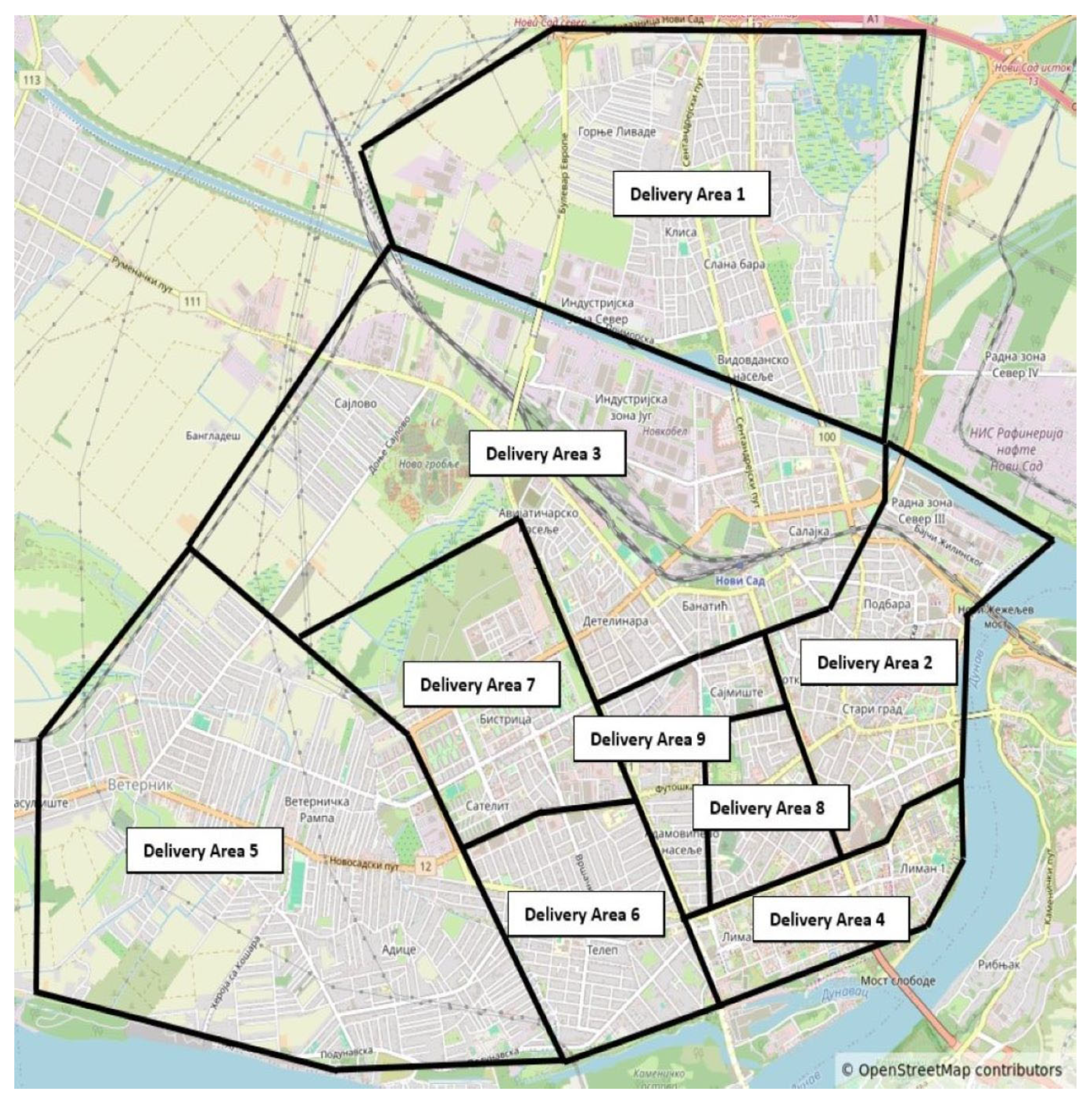
Novi Sad is the second largest city in Serbia and the capital of the autonomous province of Vojvodina. The city also represents one of the largest economic and cultural hubs in Serbia. According to the 2022 census, the population of the city proper area totals 260,438, while its urban area (including the adjacent settlements of Petrovaradin and Sremska Kamenica) comprises 306,702 inhabitants. The total land area of the city is 699 km², while its urban area spans 129.7 km². The city is located on important transport corridors, which provide significant comparative advantages. Based on the analysis of operations conducted by a private postal operator across its nine delivery areas (Figure 1) during one working month in the city of Novi Sad, a significant proportion of the distance travelled, ranging from 17% to 31%, was observed. Consequently, the question arises whether the goal of a deliveryman should be to cover as much distance as possible or if it is necessary to optimize delivery routes so that they can achieve as many deliveries or pickups as possible with the least amount of distance travelled. Of course, it is not possible to eliminate the distance travelled entirely, but it should be maintained at an optimal level. In some situations, this parameter is not directly influenced by the deliveryman, such as when they cruise to find parking spaces or encounter traffic congestion. Therefore, it should be considered to assess the available time for possible delivery completions.

The data were collected through an interview with the operator’s management, which lasted approximately three hours. During the interview, they presented their data management framework by delivery area, based on which we concluded that we could derive the necessary KPIs from their data. Through the discussion, we learned about the various challenges and issues they face. We also determined that the data for August 2024 would be sufficiently representative. The sample covered 22 working days in August 2024, during which there were no public holidays in the observed period.

4.3. Services Productivity

The basis for determining service productivity consists of identifying appropriate inputs and outputs, the relationships between them, and the system that produces services [50]. In addition to the differences compared with goods, services differ from each other in terms of intangibility, inseparability, simultaneity, and heterogeneity [51]. The peculiarity of the service sector is its labor intensity, thanks to the workforce that delivers services. Workers providing services do so under the influence of various personal, social, technical, and organizational factors [52]. Regarding services, a precisely defined set of steps is established that leads to the creation of the desired output, and the different nature of services compared with goods complicates this [53].

The productivity of a particular activity is linked to how effectively resources in the service process are transformed into economic outcomes for service providers and value for their customers [41]. In the service sector, given the nature of service processes, such systems can be viewed as open systems, given the active involvement of users in the process. Setting work tasks during working hours and the way they are performed, along with working conditions, all influence workers in the service sector. Satisfactory productivity requires appropriate planning. The ability to balance multiple tasks tends to contribute to productivity.

In the service sector, the situation is more complex because calculating both inputs and outputs is more complicated. Through inputs such as information, self-service activities, and complaints, customers participate in the service process and influence it and its output (e.g., the recipient of a shipment does not have the exact amount of money). The interaction formed between the employee at the postal operator and the customer significantly affects the efficiency of the service process.

Productivity within the service sector varies due to different mechanisms for enhancing productivity in various environments. Managers’ driving forces in improving service productivity are faster, better, and cheaper [52]. There are different approaches to improving service productivity: more diligent employee work, investment in capital equipment, automation substitution for labor, service standardization, etc. Enhancing productivity in the realm of services requires focus on both internal operational performance and external marketing elements [54].

Efforts are made to reduce variations in order to achieve better quality, ensuring a balanced approach so that each user receives a service of approximately similar quality. The wider the range of services provided by a specific operator, the more complex the control process becomes. In the postal sector, the constant quality assumption is problematic primarily due to the diverse range of services as well as the very different contents of postal items and various working environments, meaning there are no two identical deliveries. Defining productivity in services becomes more complex when determining the unit of service based on which productivity calculations will be made.

4.4. Work Environment in Last-Mile

The physical space defining the workplace can either aid or hinder workers’ efforts in terms of productivity. Regarding deliverymen, their workplace is integrated with the delivery area they cover. Therefore, factors such as vehicle condition, weather, terrain configuration, traffic conditions (congestion, available parking spaces, etc.), recipient’s mood, etc., greatly influence them.

When it comes to deliverymen, they are primarily expected to maintain the integrity of the parcel, deliver it as quickly as possible, and be courteous when interacting with the customer. During the provision of a particular service, social contact is inevitable and can affect productivity both negatively and positively. This point can be considered crucial because the overall perception of the customer’s positive or negative experience can be formed here. It is possible to develop empathy, which contributes to service quality but raises questions about productivity.

These variables shape productivity and unsuccessful delivery, the two primary indicators currently applied by postal operators in the Republic of Serbia when assessing a deliveryman’s performance. Additionally, the question arises about the number of parcels to be collected and delivered during their working hours in their delivery area. Unlike the deterministic number of parcels to be delivered, the number of parcels to be collected is stochastic (

Table 2. Productivity expressed as the number of parcels delivered per minute.

Delivery Area/ Date	Delivery Area 1	Delivery Area 2	Delivery Area 3	Delivery Area 4	Delivery Area 5	Delivery Area 6	Delivery Area 7	Delivery Area 8	Delivery Area 9
1 August 2024	0.67	0.35	0.26	0.40	0.36	0.33	0.40	0.26	0.38
2 August 2024	0.84	0.32	0.25	0.31	0.37	0.39	0.44	0.36	0.39
5 August 2024	1.07	0.55	0.30	0.70	0.71	0.81	0.93	0.53	0.85
6 August 2024	0.90	0.37	0.34	0.40	0.49	0.33	0.57	0.54	0.78
7 August 2024	0.73	0.35	0.31	0.36	0.35	0.47	0.41	0.30	0.61
8 August 2024	0.58	0.34	0.30	0.41	0.30	0.43	0.43	0.45	0.58
9 August 2024	0.75	0.26	0.25	0.56	0.32	0.33	0.44	0.29	0.88
12 August 2024	0.79	0.45	0.46	0.71	0.54	0.75	0.61	0.51	0.70
13 August 2024	0.60	0.40	0.36	0.40	0.03	0.42	0.53	0.41	0.99
14 August 2024	0.66	0.35	0.31	0.42	0.41	0.51	0.43	0.31	1.58
15 August 2024	0.74	0.35	0.24	0.40	0.49	0.45	0.38	0.35	0.51
16 August 2024	0.58	0.28	0.24	0.43	0.32	0.36	0.49	0.37	0.57
19 August 2024	0.69	0.37	0.43	0.56	0.44	0.74	0.57	0.36	1.21
20 August 2024	0.60	0.25	0.22	0.60	0.42	0.47	0.40	0.35	0.90
21 August 2024	0.62	0.28	0.24	0.52	0.34	0.39	0.50	0.31	0.52
22 August 2024	0.61	0.29	0.27	0.40	0.34	0.46	0.37	0.32	0.47
23 August 2024	0.52	0.22	0.21	0.47	0.27	0.30	0.29	0.33	0.57
26 August 2024	0.59	0.41	0.44	0.68	0.60	0.74	0.66	0.46	1.04
27 August 2024	0.76	0.28	0.29	0.46	0.33	0.37	0.49	0.50	0.79
28 August 2024	0.50	0.29	0.34	0.49	0.37	0.43	0.50	0.45	0.50
29 August 2024	0.64	0.30	0.21	0.50	0.29	0.19	0.30	0.42	0.58
30 August 2024	0.62	0.21	0.24	0.44	0.41	0.21	0.40	0.38	0.56

).

The reciprocal value of the previous table will provide us with the information about the time needed to deliver one parcel (

Table 3. Average delivery/pickup time per parcel by delivery area on a monthly basis in minutes.

Delivery Area/ Date	Delivery Area 1	Delivery Area 2	Delivery Area 3	Delivery Area 4	Delivery Area 5	Delivery Area 6	Delivery Area 7	Delivery Area 8	Delivery Area 9
1 August 2024	1.49	2.85	3.91	2.47	2.77	3.04	2.52	3.82	2.63
2 August 2024	1.18	3.09	4.07	3.24	2.69	2.56	2.28	2.81	2.53
5 August 2024	0.94	1.83	3.31	1.44	1.41	1.23	1.08	1.90	1.18
6 August 2024	1.11	2.72	2.95	2.47	2.02	3.00	1.75	1.85	1.28
7 August 2024	1.37	2.90	3.28	2.74	2.86	2.12	2.44	3.34	1.65
8 August 2024	1.71	2.93	3.35	2.45	3.38	2.33	2.34	2.21	1.74
9 August 2024	1.34	3.80	4.05	1.78	3.17	3.07	2.27	3.40	1.13
12 August 2024	1.27	2.23	2.16	1.41	1.85	1.33	1.64	1.95	1.43
13 August 2024	1.67	2.51	2.79	2.47	29.43	2.41	1.87	2.47	1.01
14 August 2024	1.52	2.83	3.18	2.36	2.45	1.97	2.33	3.18	.63
15 August 2024	1.35	2.84	4.09	2.48	2.04	2.23	2.65	2.89	1.97
16 August 2024	1.74	3.52	4.09	2.30	3.16	2.78	2.03	2.69	1.76
19 August 2024	1.45	2.71	2.34	1.77	2.26	1.35	1.75	2.80	0.83
20 August 2024	1.68	4.07	4.50	1.68	2.35	2.15	2.49	2.84	1.11
21 August 2024	1.62	3.60	4.20	1.92	2.91	2.59	1.98	3.23	1.91
22 August 2024	1.63	3.44	3.74	2.48	2.97	2.15	2.73	3.08	2.11
23 August 2024	1.92	4.55	4.86	2.14	3.67	3.30	3.44	3.01	1.75
26 August 2024	1.69	2.44	2.28	1.48	1.68	1.35	1.51	2.19	0.96
27 August 2024	1.32	3.54	3.51	2.17	3.04	2.70	2.04	2.01	1.27
28 August 2024	1.99	3.49	2.96	2.02	2.70	2.32	2.02	2.23	2.01
29 August 2024	1.56	3.29	4.69	2.01	3.40	5.21	3.32	2.37	1.73
30 August 2024	1.61	4.82	4.10	2.26	2.46	4.80	2.52	2.67	1.79

).

To evaluate productivity at 100%, it is necessary to consider the average delivery time achieved based on the delivery of express, express cash-on-delivery, and pickup shipments, along with the values of the aforementioned individual types of courier activities from the regulation [45]. Considering the total data for the observed month, the share of express shipments without cash-on-delivery is 31.69%; with cash-on-delivery, it is 21.68%, and 49.05% are shipments picked up at the location. Based on this, we find that the average time for activities related to shipments is 3.37 min. In this case, the mentioned value of 0.297 shipments per minute is equivalent to a productivity of 100%. By observing Table 2, we can notice that over 87% of productivity is higher than the estimated 100% norm recognized by the national postal operator.

If we consider all nine regions, the mathematical expectation for delivery/pickup of shipments will be around 2.44 min, with a standard deviation of 0.87 min and a median of 2.35 min. Examining individual regions showed that the average delivery/pickup times correspond to a normal distribution (

Table 4. Normal distribution of delivery/pickup times for packages.

	p-Value	M	SD	Variance	95% Confidence
Delivery Area 1	0.806	1.5075	0.2567	0.0659	(1.3936, 1.6213)
Delivery Area 2	0.503	3.1817	0.7212	0.5202	(2.8619, 3.5015)
Delivery Area 3	0.452	3.5638	0.772	0.596	(3.2215, 3.9061)
Delivery Area 4	0.35	2.1615	0.4537	0.2058	(1.9604, 2.3626)
Delivery Area 5	0.919	2.6303	0.6018	0.3622	(2.3564, 2.9043)
Delivery Area 6	0.165	2.4182	0.8124	0.66	(2.0483, 2.788)
Delivery Area 7	0.595	2.2286	0.5498	0.3022	(1.9849, 2.4724)
Delivery Area 8	0.719	2.6797	0.5464	0.2987	(2.4374, 2.9220)
Delivery Area 9	0.593	1.5643	0.5285	0.2793	(1.3300, 1.7935)

).

4.5. Failed Delivery

E-commerce retailers primarily assess postal operator performance based on the rate of unsuccessful deliveries, so unsuccessful deliveries not only incur economic loss but also significantly affect the operator’s reputation. Unsuccessful delivery is often attributed to the customer’s side, such as when the customer is absent. However, in some cases, the responsibility may lie with the operator, for instance, when a package is delivered to the wrong recipient or if the recipient refuses to accept the shipment (for example, in case of shipment damage). The failure to deliver primarily has financial implications for the e-commerce retailers (a direct consequence) and can lead to the degradation of their brand (an indirect consequence).

Predicting the outcome of delivery attempts is a complex problem, considering the diversity of factors that cannot be known in advance. Therefore, unsuccessful events are most often recorded after they occur. Operators encounter difficulties in directly capturing information regarding attempted deliveries. Consequently, they are only able to calculate the cost of unsuccessful deliveries at a later stage [55]. Inconsistency between what the e-commerce retailer promises regarding delivery times and the actual delivery realization also leads to an increase in product return rates [56].

If a delivery attempt fails, it causes a series of negative effects on all participants, including the customer, e-retailer, and postal operator, and thus affects economic, social, and environmental sustainability. The cost of unsuccessful delivery in 2020 is estimated to be USD 17.2 in the US, EUR 14.69 in Germany, and GBP 11.6 in the UK [57]. The reason for the customer’s absence is the mismatch between their lifestyle (work obligations, lifestyle) and the usual delivery times [58]. On the other hand, customers are generally unwilling to travel to retrieve their shipments [59]. In cases where parcel lockers are located at third-party locations (most commonly gas stations), customers mainly use motorized transportation, with an even more detrimental impact on the environment.

In the territory of the Republic of Serbia, postal operators have too broad a time window for delivering shipments. Operators inform customers the day before that delivery will be made between 8 a.m. and 3 p.m. The next notification is sent 5 min before the actual delivery. As statistics show, a relatively small number of customers are willing to wait “blindly,” which is supported by significant values of unsuccessful delivery attempts (

Table 5. Percentage of failed deliveries.

Delivery Area/ Date	Delivery Area 1	Delivery Area 2	Delivery Area 3	Delivery Area 4	Delivery Area 5	Delivery Area 6	Delivery Area 7	Delivery Area 8	Delivery Area 9
1 August 2024	33%	18%	16%	34%	31%	34%	52%	34%	27%
2 August 2024	16%	5%	6%	45%	23%	46%	50%	41%	25%
5 August 2024	20%	5%	24%	25%	8%	24%	29%	32%	20%
6 August 2024	7%	25%	11%	34%	12%	44%	35%	24%	21%
7 August 2024	8%	22%	7%	38%	31%	47%	27%	37%	19%
8 August 2024	12%	4%	11%	40%	37%	29%	32%	44%	24%
9 August 2024	4%	3%	18%	27%	35%	37%	32%	38%	19%
12 August 2024	15%	11%	10%	41%	23%	28%	29%	29%	28%
13 August 2024	13%	12%	13%	38%	16%	37%	20%	30%	19%
14 August 2024	19%	12%	5%	39%	16%	33%	27%	46%	35%
15 August 2024	3%	19%	17%	36%	18%	32%	26%	37%	24%
16 August 2024	4%	10%	19%	41%	17%	41%	29%	28%	22%
19 August 2024	15%	1%	20%	35%	36%	32%	25%	37%	21%
20 August 2024	10%	17%	34%	36%	23%	23%	33%	29%	20%
21 August 2024	19%	26%	13%	33%	24%	39%	32%	31%	32%
22 August 2024	16%	16%	13%	46%	35%	27%	26%	32%	22%
23 August 2024	16%	18%	11%	40%	32%	28%	33%	38%	32%
26 August 2024	17%	9%	14%	38%	21%	20%	27%	39%	23%
27 August 2024	2%	14%	26%	40%	31%	32%	26%	23%	13%
28 August 2024	11%	13%	12%	34%	27%	34%	27%	28%	22%
29 August 2024	18%	17%	24%	34%	32%	44%	35%	39%	31%
30 August 2024	11%	27%	20%	36%	29%	43%	43%	37%	26%

).

Various alternatives are sought to address the issue of unsuccessful delivery: parcel lockers, parcel shops, or third-party locations with contracts with the postal operator, rerouting of shipments, choice of delivery time slots, etc. However, some solutions, in addition to increasing the percentage of successfully delivered shipments, may have a negative impact on shipment consolidation and routing efficiency [60]. First-time delivery failure rates vary from 10% to 50% [58]. In the observed regions on a monthly basis, failed delivery rates ranged from 13% to 37%, although daily rates sometimes exceeded 40%. This raises the question of what failure rates e-retailers can tolerate.

4.6. Application of IRN MCDM Model for Ranking Delivery Zones

Based on available results obtained from a postal operator, the following Key Performance Indicators (KPIs) have been selected: productivity, failure rate, number of shipments, distance travelled, and CO₂ emissions per shipment (

Table 6. Initial decision-making quantitative data.

Delivery Area	Productivity (Shipments/min)	Failure Rate	Number of Shipments	Distance Travelled (km)	CO2 Emissions per Shipment (g)
1	0.68	0.13	4641	1212	164
2	0.33	0.14	2349	1009	268
3	0.29	0.16	2111	984	294
4	0.48	0.37	3340	1125	213
5	0.38	0.29	2693	1033	253
6	0.43	0.34	2934	1232	262
7	0.46	0.32	2583	1830	426
8	0.39	0.34	2754	1050	240
9	0.67	0.24	3436	2062	378
Hypothetical	0.297	0.26	2045	1282	450

). A hypothetical scenario has been developed where, according to the methodology of the PE Post of Serbia, productivity is at 100%. This hypothetical scenario is introduced to evaluate the current state of delivery areas relative to 100% productivity.

Considering that the criteria—i.e., the KPIs in this case—do not have the same level of importance or influence on the alternative solutions, it is first necessary to determine the weights of the KPIs used in the evaluation of delivery zones related to last-mile logistics. The calculation and application of the IRN-OWCM algorithm are presented in detail below, as this represents a novel approach. As part of the research, four experts with significant experience in the field were consulted. Based on the quantitative data provided in Table 6, they evaluated both the criteria and the delivery zones. The linguistic variables created through expert assessment are first introduced and presented in

Table 7. Linguistic matrix for IRN OWCM.

E1	C1	C2	C3	C4	C5	E2	C1	C2	C3	C4	C5
A1	NOD	NOD	NOD	MD	NOD	A1	NOD	NOD	NOD	MHD	NOD
A2	HD	NOD	HD	SD	HD	A2	VHD	NOD	HD	SD	MD
A3	VHD	SD	HD	NOD	HD	A3	EHD	SD	VHD	NOD	MHD
A4	MD	HD	MD	MD	MD	A4	MD	EHD	MD	MD	SD
A5	HD	MHD	MHD	SD	MHD	A5	HD	MHD	MHD	SD	MD
A6	MHD	HD	MHD	MD	MHD	A6	MHD	VHD	MHD	MHD	MD
A7	MD	HD	MHD	HD	EHD	A7	MHD	VHD	MHD	VHD	VHD
A8	HD	HD	MHD	SD	MHD	A8	HD	VHD	MHD	SD	MD
A9	NOD	MHD	MD	VHD	VHD	A9	NOD	MHD	MD	EHD	VHD
A10	VHD	MHD	HD	MD	EHD	A10	EHD	MHD	VHD	MHD	VHD
E3	C1	C2	C3	C4	C5	E4	C1	C2	C3	C4	C5
A1	NOD	NOD	NOD	MHD	NOD	A1	NOD	NOD	NOD	MHD	NOD
A2	VHD	NOD	HD	SD	MHD	A2	HD	NOD	VHD	NOD	MHD
A3	VHD	SD	EHD	NOD	MHD	A3	VHD	NOD	EHD	NOD	MHD
A4	MD	VHD	MD	MD	SD	A4	MHD	HD	MD	MD	SD
A5	HD	MHD	MHD	SD	MD	A5	HD	MD	MHD	SD	MD
A6	MHD	VHD	MHD	MHD	MD	A6	MHD	HD	MHD	MD	MD
A7	MHD	HD	MHD	VHD	EHD	A7	MHD	MHD	MHD	VHD	EHD
A8	HD	VHD	MHD	SD	MD	A8	HD	HD	MHD	SD	MD
A9	NOD	MD	MD	EHD	VHD	A9	NOD	SD	MD	EHD	VHD
A10	VHD	MD	EHD	MHD	EHD	A10	VHD	SD	EHD	MHD	VHD

.

Based on Table 1, the linguistic variables were transformed into interval numbers, as shown in the

Table 8. Matrix transformed into interval numbers.

E1	C1		C2		C3		C4		C5		E2	C1		C2		C3		C4		C5
A1	1	1	1	1	1	1	2	3	1	1	A1	1	1	1	1	1	1	3	4	1	1
A2	4	5	1	1	4	5	1	2	4	5	A2	5	6	1	1	4	5	1	2	2	3
A3	5	6	1	2	4	5	1	1	4	5	A3	6	7	1	2	5	6	1	1	3	4
A4	2	3	4	5	2	3	2	3	2	3	A4	2	3	6	7	2	3	2	3	1	2
A5	4	5	3	4	3	4	1	2	3	4	A5	4	5	3	4	3	4	1	2	2	3
A6	3	4	4	5	3	4	2	3	3	4	A6	3	4	5	6	3	4	3	4	2	3
A7	2	3	4	5	3	4	4	5	6	7	A7	3	4	5	6	3	4	5	6	5	6
A8	4	5	4	5	3	4	1	2	3	4	A8	4	5	5	6	3	4	1	2	2	3
A9	1	1	3	4	2	3	5	6	5	6	A9	1	1	3	4	2	3	6	7	5	6
A10	5	6	3	4	4	5	2	3	6	7	A10	6	7	3	4	5	6	3	4	5	6
E3	C1		C2		C3		C4		C5		E4	C1		C2		C3		C4		C5
A1	1	1	1	1	1	1	3	4	1	1	A1	1	1	1	1	1	1	3	4	1	1
A2	5	6	1	1	4	5	1	2	3	4	A2	4	5	1	1	5	6	1	1	3	4
A3	5	6	1	2	6	7	1	1	3	4	A3	5	6	1	1	6	7	1	1	3	4
A4	2	3	5	6	2	3	2	3	1	2	A4	3	4	4	5	2	3	2	3	1	2
A5	4	5	3	4	3	4	1	2	2	3	A5	4	5	2	3	3	4	1	2	2	3
A6	3	4	5	6	3	4	3	4	2	3	A6	3	4	4	5	3	4	2	3	2	3
A7	3	4	4	5	3	4	5	6	6	7	A7	3	4	3	4	3	4	5	6	6	7
A8	4	5	5	6	3	4	1	2	2	3	A8	4	5	4	5	3	4	1	2	2	3
A9	1	1	2	3	2	3	6	7	5	6	A9	1	1	1	2	2	3	6	7	5	6
A10	5	6	2	3	6	7	3	4	6	7	A10	5	6	1	2	6	7	3	4	5	6

. This represents the first prerequisite for applying the developed algorithm, i.e., the conversion into interval rough numbers.

All procedures of transformation linguistics values in interval rough numbers have been shown as follows.

IRN consists of two rough sequences; two classes of objects are identified. We take the example of the third criterion C3 and alternative A10: $A_{10-3}=\left\{4,5,6,6\right\}$ and $A_{10-3}\prime =\left\{5,6,7,7\right\}$. It is necessary to form rough sequences for each specified class of objects. For the stated example, they are obtained for the first class of objects as follows:

$$\underset{¯}{Lim}(4)=4, \overline{Lim}(4)={\displaystyle \frac{1}{4}}(4+5+6+6)=5.25; IRN(4)=[4,5.25]$$

$$\underset{¯}{Lim}(5)={\displaystyle \frac{1}{2}}\left(4+5\right)=4.50, \overline{Lim}(5)={\displaystyle \frac{1}{3}}(5+6+6)=5.67; IRN(5)=[4.50,5.67]$$

$$\underset{¯}{Lim}(6)={\displaystyle \frac{1}{4}}(4+5+6+6)=5.25, \overline{Lim}(6)=6; IRN(6)=[5.25,6]$$

For the second class of objects, the following is obtained:

$$\underset{¯}{Lim}(5)=5, \overline{Lim}(5)={\displaystyle \frac{1}{4}}(5+6+7+7)=6.25; IRN(5)=[5,6.25]$$

$$\underset{¯}{Lim}(6)={\displaystyle \frac{1}{2}}\left(5+6\right)=5.50, \overline{Lim}(6)={\displaystyle \frac{1}{3}}(6+7+7)=6.67; IRN(6)=[5.50,6.67]$$

$$\underset{¯}{Lim}(7)={\displaystyle \frac{1}{4}}(5+6+7+7)=6.25, \overline{Lim}(7)={\displaystyle \frac{1}{2}}\left(7+7\right)=7; IRN(7)=[6.25,7]$$

Based on the rough sequences, interval rough numbers are obtained:

$$\begin{gathered} IRN(E1)=\left(\left[4,5.25\right],\left[5,6.25\right]\right), IRN(E2)=\left(\left[4.50,5.67\right],\left[5.50,6.67\right]\right), \\ IRN(E3)=\left(\left[5.25,6\right],\left[6.25,7\right]\right),\mathrm{and} IRN(E4)=\left(\left[5.25,6\right],\left[6.25,7\right]\right). \end{gathered}$$

An example of obtaining a final interval number $IRN{A}_{10-3}=\left[4.75,5.73\right],\left[5.75,6.73\right]$ is:

$$\begin{array}{ll}IR{N}^L{A}_{10-3}={\displaystyle \frac{1}{4}}(4+4.50+5.25+5.25)=4.75\hspace{1em}& R{N}^L{A}_{ 10-3}\prime ={\displaystyle \frac{1}{4}}(5+5.50+6.25+6.25)=5.75\\ R{N}^U{A}_{10-3}={\displaystyle \frac{1}{4}}(5.25+5.67+6+6)=5.73,& R{N}^U{A}_{10-3}\prime ={\displaystyle \frac{1}{4}}(6.25+6.67+7+7)=6.73\end{array}$$

The third step involves defining the initial IRN(IM_ij) matrix while respecting the basic rules and operations of rough number theory. The complete IRN(IMij) matrix is presented in

Table 9. Initial decision matrix—IRN OWCM.

	C1	C2	C3	C4	C5
A1	[1, 1], [1, 1]	[1, 1], [1, 1]	[1, 1], [1, 1]	[2.56, 2.94], [3.56, 3.94]	[1, 1], [1, 1]
A2	[4.25, 4.75], [5.25, 5.75]	[1, 1], [1, 1]	[4.06, 4.44], [5.06, 5.44]	[1, 1], [1.56, 1.94]	[2.59, 3.42], [3.59, 4.42]
A3	[5.06, 5.44], [6.06, 6.44]	[1, 1], [1.56, 1.94]	[4.75, 5.73], [5.75, 6.73]	[1, 1], [1, 1]	[3.06, 3.44], [4.06, 4.44]
A4	[2.06, 2.44], [3.06, 3.44]	[4.27, 5.25], [5.27, 6.25]	[2, 2], [3, 3]	[2, 2], [3, 3]	[1.06, 1.44], [2.06, 2.44]
A5	[4, 4], [5, 5]	[2.56, 2.94], [3.56, 3.94]	[3, 3], [4, 4]	[1, 1], [2, 2]	[2.06, 2.44], [3.06, 3.44]
A6	[3, 3], [4, 4]	[4.25, 4.75], [5.25, 5.75]	[3, 3], [4, 4]	[2.25, 2.75], [3.25, 3.75]	[2.06, 2.44], [3.06, 3.44]
A7	[2.56, 2.94], [3.56, 3.94]	[3.59, 4.42], [4.59, 5.42]	[3, 3], [4, 4]	[4.56, 4.94], [5.56, 5.94]	[5.56, 5.94], [6.56, 6.94]
A8	[4, 4], [5, 5]	[4.25, 4.75], [5.25, 5.75]	[3, 3], [4, 4]	[1, 1], [2, 2]	[2.06, 2.44], [3.06, 3.44]
A9	[1, 1], [1, 1]	[1.75, 2.73], [2.75, 3.73]	[2, 2], [3, 3]	[5.56, 5.94], [6.56, 6.94]	[5, 5], [6, 6]
A10	[5.06, 5.44], [5.59, 6.42]	[1.75, 2.73], [2.75, 3.73]	[4.75, 5.73], [5.75, 6.73]	[2.56, 2.94], [3.56, 3.94]	[5.25, 5.75], [6.25, 6.75]

.

In the fourth step, the normalization procedure of the IRN(IM_ij) matrix is performed according to Equation (2), as illustrated by the following example:$IRN(n_{41})=\left(\left[{\displaystyle \frac{2.06}{6.44}},{\displaystyle \frac{2.44}{6.06}}\right],\left[{\displaystyle \frac{3.06}{5.44}},{\displaystyle \frac{3.44}{5.06}}\right]\right)=\left(\left[0.320,0.403\right],\left[0.563,0.680\right]\right)$ by obtaining the normalized IRN(NM_ij) matrix (

Table 10. Normalized IRN OWCM matrix.

	C1	C2	C3	C4	C5
A1	[0.16, 0.17], [0.18, 0.2]	[0.16, 0.19], [0.19, 0.23]	[0.15, 0.17], [0.17, 0.21]	[0.37, 0.45], [0.6, 0.71]	[0.14, 0.15], [0.17, 0.18]
A2	[0.66, 0.78], [0.97, 1.14]	[0.16, 0.19], [0.19, 0.23]	[0.6, 0.77], [0.88, 1.15]	[0.14, 0.15], [0.26, 0.35]	[0.37, 0.52], [0.6, 0.79]
A3	[0.79, 0.9], [1.11, 1.27]	[0.16, 0.19], [0.3, 0.45]	[0.71, 1], [1, 1.42]	[0.14, 0.15], [0.17, 0.18]	[0.44, 0.52], [0.68, 0.8]
A4	[0.32, 0.4], [0.56, 0.68]	[0.68, 1], [1, 1.46]	[0.3, 0.35], [0.52, 0.63]	[0.29, 0.3], [0.51, 0.54]	[0.15, 0.22], [0.35, 0.44]
A5	[0.62, 0.66], [0.92, 0.99]	[0.41, 0.56], [0.68, 0.92]	[0.45, 0.52], [0.7, 0.84]	[0.14, 0.15], [0.34, 0.36]	[0.3, 0.37], [0.52, 0.62]
A6	[0.47, 0.5], [0.74, 0.79]	[0.68, 0.9], [1, 1.35]	[0.45, 0.52], [0.7, 0.84]	[0.32, 0.42], [0.55, 0.67]	[0.3, 0.37], [0.52, 0.62]
A7	[0.4, 0.49], [0.65, 0.78]	[0.57, 0.84], [0.87, 1.27]	[0.45, 0.52], [0.7, 0.84]	[0.66, 0.75], [0.94, 1.07]	[0.8, 0.91], [1.1, 1.25]
A8	[0.62, 0.66], [0.92, 0.99]	[0.68, 0.9], [1, 1.35]	[0.45, 0.52], [0.7, 0.84]	[0.14, 0.15], [0.34, 0.36]	[0.3, 0.37], [0.52, 0.62]
A9	[0.16, 0.17], [0.18, 0.2]	[0.28, 0.52], [0.52, 0.87]	[0.3, 0.35], [0.52, 0.63]	[0.8, 0.91], [1.1, 1.25]	[0.72, 0.76], [1.01, 1.08]
A10	[0.79, 0.9], [1.03, 1.27]	[0.28, 0.52], [0.52, 0.87]	[0.71, 1], [1, 1.42]	[0.37, 0.45], [0.6, 0.71]	[0.76, 0.88], [1.05, 1.21]

).

In the fifth step, it is necessary to calculate the average score of the standardized decision matrix IRN(Avs_j), and prior to that, the summed values of the normalized IRN(NM_ij) matrix, resulting in the IRN(SM_j) matrix:

$$\begin{array}{l}IRN(S{M}_j)=\left(\left[4.97,5.61\right],\left[7.26,8.3\right]\right),\left(\left[4.07,5.8\right],\left[6.28,9.02\right]\right),\left(\left[4.54,5.72\right],\left[6.9,8.82\right]\right),\\ \left(\left[3.38,3.89\right],\left[5.4,6.2\right]\right),\left(\left[4.28,5.08\right],\left[6.52,7.61\right]\right)\end{array}$$

The IRN(Avs_j) matrix is obtained as follows:

$$IRN(av{s}_1)=\left(\left[{\displaystyle \frac{1}{10\times 8.298}},{\displaystyle \frac{1}{10\times 7.265}}\right],\left[{\displaystyle \frac{1}{10\times 5.612}},{\displaystyle \frac{1}{10\times 4.967}}\right]\right)=\left(\left[0.012,0.014\right],\left[0.018,0.020\right]\right)$$

$$\begin{array}{l}IRN(Av{s}_j)=\left(\left[0.012,0.014\right],\left[0.018,0.020\right]\right),\left(\left[0.011,0.016\right],\left[0.017,0.025\right]\right),\\ \left(\left[0.011,0.014\right],\left[0.017,0.022\right]\right),\left(\left[0.016,0.019\right],\left[0.026,0.030\right]\right),\left(\left[0.013,0.015\right],\left[0.020,0.023\right]\right)\end{array}$$

Determines the degree of preference variation, and its corresponding value IRN(DPV_ij) is obtained as follows:

$$IRN(dp{v}_{21})=\left(\begin{array}{l}\left[{\left(0.660-0.020\right)}^2,{\left(0.784-0.018\right)}^2\right],\\ \left[{\left(0.965-0.014\right)}^2,{\left(1.136-0.012\right)}^2\right]\end{array}\right)=\left(\left[0.409,0.587\right],\left[0.905,1.264\right]\right)$$

The final IRN(DPV_ij) is presented in

Table 11. IRN(DPV_ij) matrix.

	C1	C2	C3	C4	C5
A1	[0.02, 0.02], [0.03, 0.03]	[0.02, 0.03], [0.03, 0.05]	[0.02, 0.02], [0.03, 0.04]	[0.12, 0.18], [0.34, 0.48]	[0.01, 0.02], [0.02, 0.03]
A2	[0.41, 0.59], [0.9, 1.26]	[0.02, 0.03], [0.03, 0.05]	[0.34, 0.57], [0.75, 1.29]	[0.01, 0.02], [0.06, 0.11]	[0.12, 0.25], [0.35, 0.61]
A3	[0.59, 0.77], [1.21, 1.59]	[0.02, 0.03], [0.08, 0.2]	[0.47, 0.96], [0.98, 1.98]	[0.01, 0.02], [0.02, 0.03]	[0.17, 0.25], [0.45, 0.62]
A4	[0.09, 0.15], [0.3, 0.45]	[0.43, 0.96], [0.98, 2.11]	[0.08, 0.11], [0.26, 0.38]	[0.07, 0.08], [0.24, 0.27]	[0.02, 0.04], [0.11, 0.18]
A5	[0.36, 0.41], [0.82, 0.95]	[0.15, 0.29], [0.44, 0.83]	[0.18, 0.25], [0.47, 0.69]	[0.01, 0.02], [0.1, 0.12]	[0.07, 0.12], [0.25, 0.37]
A6	[0.2, 0.23], [0.52, 0.61]	[0.43, 0.78], [0.97, 1.78]	[0.18, 0.25], [0.47, 0.69]	[0.09, 0.15], [0.28, 0.43]	[0.07, 0.12], [0.25, 0.37]
A7	[0.14, 0.22], [0.41, 0.59]	[0.3, 0.67], [0.74, 1.58]	[0.18, 0.25], [0.47, 0.69]	[0.39, 0.53], [0.84, 1.11]	[0.6, 0.78], [1.19, 1.53]
A8	[0.36, 0.41], [0.82, 0.95]	[0.43, 0.78], [0.97, 1.78]	[0.18, 0.25], [0.47, 0.69]	[0.01, 0.02], [0.1, 0.12]	[0.07, 0.12], [0.25, 0.37]
A9	[0.02, 0.02], [0.03, 0.03]	[0.07, 0.25], [0.26, 0.74]	[0.08, 0.11], [0.26, 0.38]	[0.6, 0.77], [1.18, 1.52]	[0.49, 0.55], [0.99, 1.14]
A10	[0.59, 0.77], [1.03, 1.58]	[0.07, 0.25], [0.26, 0.74]	[0.47, 0.96], [0.98, 1.98]	[0.12, 0.18], [0.34, 0.48]	[0.54, 0.73], [1.08, 1.44]

.

Next, the previous matrix is summed column-wise to obtain the IRN(SDPV_j) matrix:

$\begin{array}{l}IRN(SDP{V}_j)=\left(\left[2.771,3.598\right],\left[6.073,8.047\right]\right),\left(\left[1.929,4.080\right],\left[4.744,9.875\right]\right),\\ \left(\left[2.159,3.746\right],\left[5.124,8.806\right]\right),\left(\left[1.426,1.957\right],\left[3.496,4.665\right]\right),\left(\left[2.181,3.006\right],\left[4.927,6.641\right]\right)\end{array}$

In the final step, the calculation of the IRN criterion weights w_j is performed as illustrated by the example:

$w_1=\left(\left[{\displaystyle \frac{2.771}{38.035}},{\displaystyle \frac{3.598}{24.363}}\right],\left[{\displaystyle \frac{6.073}{16.387}},{\displaystyle \frac{8.047}{10.465}}\right]\right)=\left(\left[0.073,0.148\right],\left[0.371,0.769\right]\right)$, and the final IRN weights of all criteria are:

$$\begin{array}{l}{w}_1=\left(\left[0.073,0.148\right],\left[0.371,0.769\right]\right),w_2=\left(\left[0.051,0.167\right],\left[0.289,0.944\right]\right),\\ w_3=\left(\left[0.057,0.154\right],\left[0.313,0.841\right]\right),w_4=\left(\left[0.037,0.080\right],\left[0.213,0.446\right]\right),\\ w_5=\left(\left[0.057,0.123\right],\left[0.301,0.635\right]\right)\end{array}$$

After calculating the criterion weights using the developed IRN OWCM, the most influential KPI is the one related to the failure rate. The third KPI, number of shipments, and the first KPI, related to productivity, have nearly equal values, which are slightly lower compared with the most influential criterion.

The next part of the research involves applying the IRN AROMAN method to assess the efficiency of urban zones related to last-mile delivery. First, the experts evaluated the delivery zones using linguistic variables, as shown in

Table 12. Initial linguistic matrix in IRN AROMAN.

	E1					E2
	C1	C2	C3	C4	C5	C1	C2	C3	C4	C5
A1	VVH	VVH	VVH	MH	VVH	VVH	VH	VVH	M	VVH
A2	L	VVH	VL	VVH	M	VL	VH	VVL	VH	M
A3	VL	VH	VVL	VVH	M	VL	H	VVL	VH	M
A4	M	L	MH	H	H	M	VL	MH	MH	H
A5	ML	M	L	VH	MH	ML	ML	L	H	MH
A6	M	L	ML	MH	MH	M	VL	ML	M	MH
A7	M	ML	L	L	L	M	L	L	VL	ML
A8	ML	L	ML	VH	MH	ML	VL	ML	H	MH
A9	VVH	MH	MH	VVL	ML	VVH	M	MH	VVL	ML
A10	VL	MH	VVL	MH	L	VL	M	VVL	M	ML
	E3					E4
	C1	C2	C3	C4	C5	C1	C2	C3	C4	C5
A1	VVH	VVH	VH	MH	VH	VH	VVH	VVH	MH	VH
A2	L	VVH	VVL	VVH	M	VL	VVH	VVL	VVH	M
A3	VVL	VVH	VVL	VVH	M	VVL	VVH	VVL	VVH	M
A4	M	L	M	H	H	ML	L	MH	H	H
A5	ML	M	VL	VVH	MH	L	M	L	VH	MH
A6	M	L	L	MH	MH	ML	L	ML	MH	MH
A7	M	ML	VL	L	L	ML	ML	L	VL	L
A8	ML	L	L	VH	MH	L	L	ML	VH	MH
A9	VVH	MH	M	VVL	ML	VH	MH	M	VVL	ML
A10	VVL	MH	VVL	MH	L	VVL	MH	VVL	MH	L

, followed by the quantitative matrix with interval numbers, presented in

Table 13. IRN AROMAN matrix with interval numbers.

E1	C1		C2		C3		C4		C5		E2	C1		C2		C3		C4		C5
A1	8	9	8	9	8	9	5	6	8	9	A1	8	9	7	8	8	9	4	5	8	9
A2	2	3	8	9	1	2	8	9	4	5	A2	1	2	7	8	1	1	7	8	4	5
A3	1	2	7	8	1	1	8	9	4	5	A3	1	2	6	7	1	1	7	8	4	5
A4	4	5	2	3	5	6	6	7	6	7	A4	4	5	1	2	5	6	5	6	6	7
A5	3	4	4	5	2	3	7	8	5	6	A5	3	4	3	4	2	3	6	7	5	6
A6	4	5	2	3	3	4	5	6	5	6	A6	4	5	1	2	3	4	4	5	5	6
A7	4	5	3	4	2	3	2	3	2	3	A7	4	5	2	3	2	3	1	2	3	4
A8	3	4	2	3	3	4	7	8	5	6	A8	3	4	1	2	3	4	6	7	5	6
A9	8	9	5	6	5	6	1	1	3	4	A9	8	9	4	5	5	6	1	1	3	4
A10	1	2	5	6	1	1	5	6	2	3	A10	1	2	4	5	1	1	4	5	3	4
E3	C1		C2		C3		C4		C5		E4	C1		C2		C3		C4		C5
A1	8	9	8	9	7	8	5	6	7	8	A1	7	8	8	9	8	9	5	6	7	8
A2	2	3	8	9	1	1	8	9	4	5	A2	1	2	8	9	1	1	8	9	4	5
A3	1	1	8	9	1	1	8	9	4	5	A3	1	1	8	9	1	1	8	9	4	5
A4	4	5	2	3	4	5	6	7	6	7	A4	3	4	2	3	5	6	6	7	6	7
A5	3	4	4	5	1	2	8	9	5	6	A5	2	3	4	5	2	3	7	8	5	6
A6	4	5	2	3	2	3	5	6	5	6	A6	3	4	2	3	3	4	5	6	5	6
A7	4	5	3	4	1	2	2	3	2	3	A7	3	4	3	4	2	3	1	2	2	3
A8	3	4	2	3	2	3	7	8	5	6	A8	2	3	2	3	3	4	7	8	5	6
A9	8	9	5	6	4	5	1	1	3	4	A9	7	8	5	6	4	5	1	1	3	4
A10	1	1	5	6	1	1	5	6	2	3	A10	1	1	5	6	1	1	5	6	2	3

.

By applying the IRN-AROMAN method in combination with the criterion weights obtained from the IRN-OWCM method, the final results were produced (

Table 14. Final results of assessment of delivery zones.

$\mathit{I}\mathit{R}\mathit{N}({\mathit{Џ}}_{\mathit{i}})={\displaystyle \sum _{\mathit{j}=1}^{\mathit{n}}\left({\mathit{Б}}_{\mathit{i}\mathit{j}}\right)}$	$\mathit{I}\mathit{R}\mathit{N}({\mathit{Ч}}_{\mathit{i}})={\left({\mathit{М}}_{\mathit{i}}\right)}^{\mathsf{\gamma }}+{\left({\mathit{Џ}}_{\mathit{i}}\right)}^{\left(1-\mathsf{\gamma }\right)}$	AV	Rank
[0.081, 0.216], [0.537, 1.448]	[0.284, 0.465], [0.733, 1.203]	0.671	1	A1
[0.036, 0.106], [0.272, 0.79]	[0.191, 0.326], [0.522, 0.889]	0.482	4	A2
[0.034, 0.099], [0.241, 0.72]	[0.184, 0.315], [0.491, 0.849]	0.460	6	A3
[0.043, 0.11], [0.315, 0.823]	[0.206, 0.331], [0.561, 0.907]	0.501	3	A4
[0.034, 0.094], [0.27, 0.738]	[0.185, 0.307], [0.52, 0.859]	0.468	5	A5
[0.032, 0.084], [0.257, 0.677]	[0.18, 0.291], [0.507, 0.823]	0.450	8	A6
[0.018, 0.058], [0.178, 0.526]	[0.135, 0.24], [0.422, 0.725]	0.381	9	A7
[0.032, 0.084], [0.258, 0.679]	[0.18, 0.291], [0.508, 0.824]	0.451	7	A8
[0.046, 0.124], [0.327, 0.89]	[0.215, 0.352], [0.571, 0.943]	0.521	2	A9
[0.018, 0.057], [0.152, 0.473]	[0.134, 0.238], [0.39, 0.688]	0.363	10	A10

), identifying the most appropriate delivery zones based on the previously established KPIs.

Based on the integration of the IRN OWCM and IRN AROMAN methods, delivery zone A1 is ranked as the most efficient (1st place), confirming its optimality with respect to the defined KPI indicators. A1 has one of the highest productivity levels (0.68 shipments/min), the lowest failure rate (0.13), and a moderate CO₂ emission per shipment (164 g), indicating an efficient and environmentally sustainable delivery model. Its overall value, considering the number of shipments and distance traveled, demonstrates a strong balance between operational efficiency and sustainability.

Areas such as A9 (2nd place) and A4 (3rd place) also demonstrate solid performance, though not to the extent of A1. Lower-ranked zones (A6, A7, A8) reveal more significant operational challenges, particularly regarding distance and environmental impact, making them less favorable for efficient last-mile delivery.

However, when a delivery area consistently performs at a high level, there is a potential risk of overloading due to increased routing pressure. To prevent capacity saturation and ensure service stability, reorganization or redistribution of delivery areas may be necessary as a strategic solution.

In some developed approaches, there exists a certain inconsistency of expert judgments and results obtained using the proposed model. Our developed IRN MCDM model enables consistency of the obtained results with the initial step, the assessment made by experts.

5. Comparative Analysis and Sensitivity Analysis

A very important aspect of the decision-making process is the verification of the obtained results through various types of tests. The following section presents analyses related to the following: a comparative analysis with other IRN MCDM models, an analysis of simulated new KPI weights, variations in the α and γ coefficients, as well as calculated statistical correlation tests.

5.1. Comparative Analysis

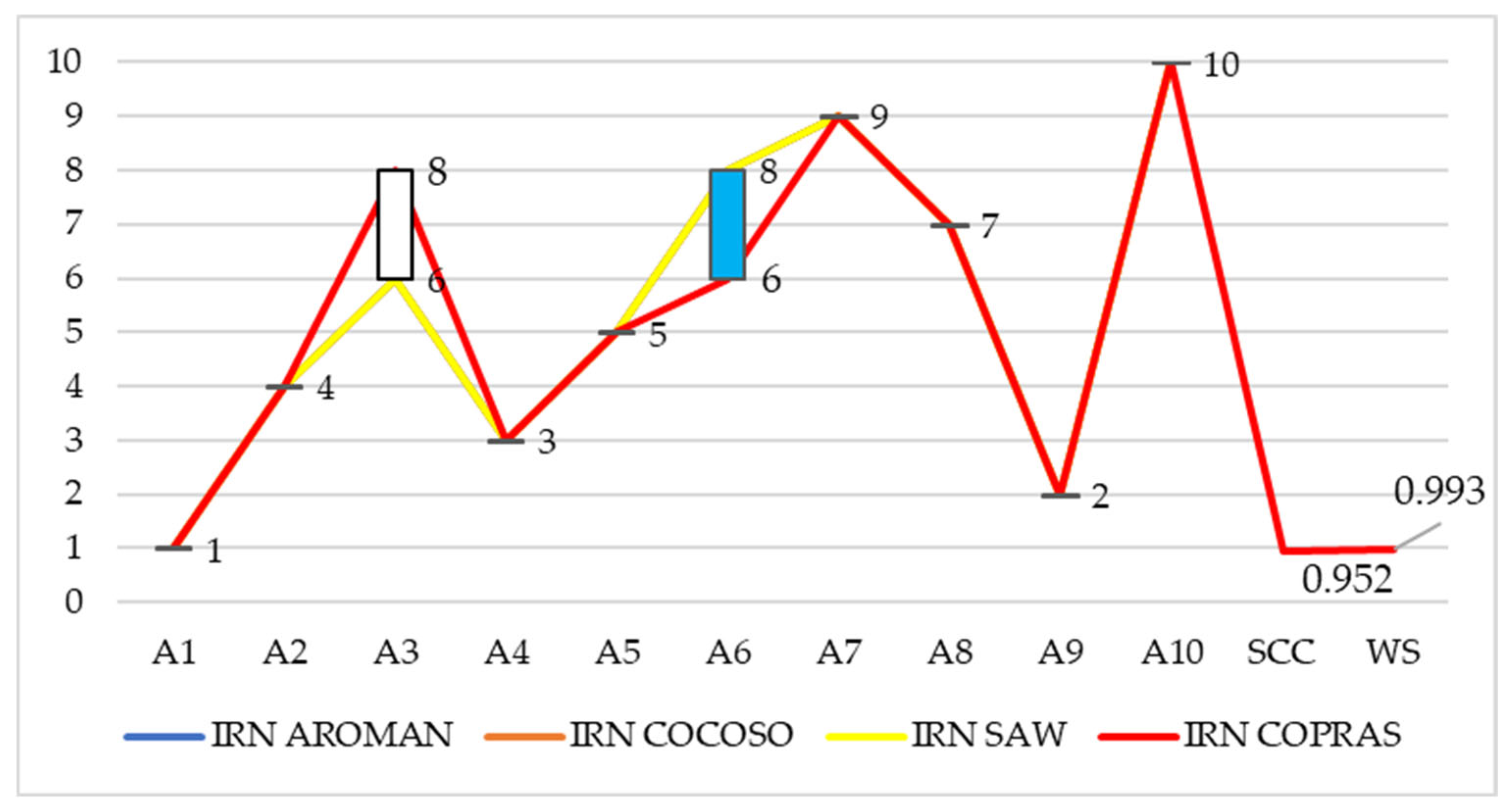
Verification of rankings in MCDM models is performed by reproducing the initial model using different methods, as is the case in this research. The original rankings obtained using the IRN AROMAN method were validated against the following IRN MCDM methods: IRN COCOSO, IRN SAW, and IRN COPRAS, with the results shown in Figure 2.

The results presented in Figure 2 show that the original rankings were confirmed by the IRN COCOSO and IRN SAW methods, while the application of the IRN COPRAS algorithm reveals differences in the rankings of certain last-mile delivery zones. Specifically, two urban areas, A3 and A6, shifted their rankings by two positions: A3: 6 >>> 8, A6: 8 >>> 6. Overall, considering the complete comparative analysis, it can be concluded that the originally obtained results and rankings are largely confirmed.

5.2. Sensitivity Analysis

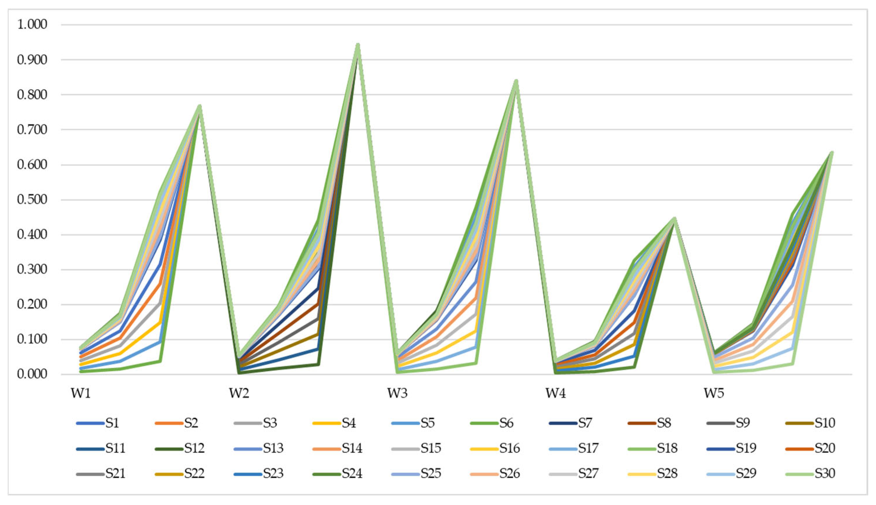
Figure 3 presents newly defined KPI values to determine whether changing the importance of individual criteria affects the final results.

Using Equation (29), a total of 30 scenarios were formed.

$$W_{n\beta }=\left(1-W_{n\alpha }\right){\displaystyle \frac{W_{\beta }}{\left(1-W_n\right)}}$$

(29)

In scenarios S1–S6, the first criterion was changed; criterion C2 was changed in scenarios S7–S12; criterion C3 was changed in scenarios S13–S18; criterion C4 was changed in scenarios S19–S24; and criterion C5 was changed in scenarios S25–S30. In Equation (29), $W_{n\beta }$ marks the new value of criteria C2–C5; for scenarios S1–S6, etc. marks the corrected value of criterion C1; in the first group of scenarios (S1–S6), $W_{\beta }$ represents the original value of the criterion considered; and $W_n$ represents the original value of the criterion whose value is reduced. The newly simulated values are presented across 30 scenarios, involving variations ranging from 15% to 90%, where the reduction in the weight of one criterion is redistributed among the others. This means, for example, that if the weight of the first criterion is reduced, the weights of the remaining criteria increase. Due to the nature of rough number theory, the upper bound of the right interval number remains unchanged. The defined criterion values for all 30 scenarios are then reapplied within the IRN OWCM–IRN AROMAN model to identify potential changes in the results, as illustrated in Figure 4.

The new rankings, generated after running 30 revised models, demonstrate the model’s sensitivity to changes in the importance of input parameters (i.e., KPIs), as ranking changes occur in 60% of the scenarios. No changes are observed in the last six scenarios, where the value of the fifth criterion is reduced. It is important to note that delivery zone A1 consistently remains in first place—that is, it maintains the best performance regardless of the value of any individual criterion. This suggests that changes in the value of the fifth criterion have no effect on its ranking. From this perspective, the stability of the top-performing zone can be confirmed. To provide a clearer view of the ranking changes, only the scenarios in which any change occurred are highlighted and presented in Figure 5.

The variations in rankings shown in Figure 5 indicate that changes most often involve a shift of only one position, either upward or downward. When examining the second-best-ranked zone, it can be observed that productivity has the greatest influence on the ranking changes of A9. Specifically, when the weight of the productivity factor is reduced, this alternative drops by as many as three positions in the sixth set.

5.3. Correlation Test

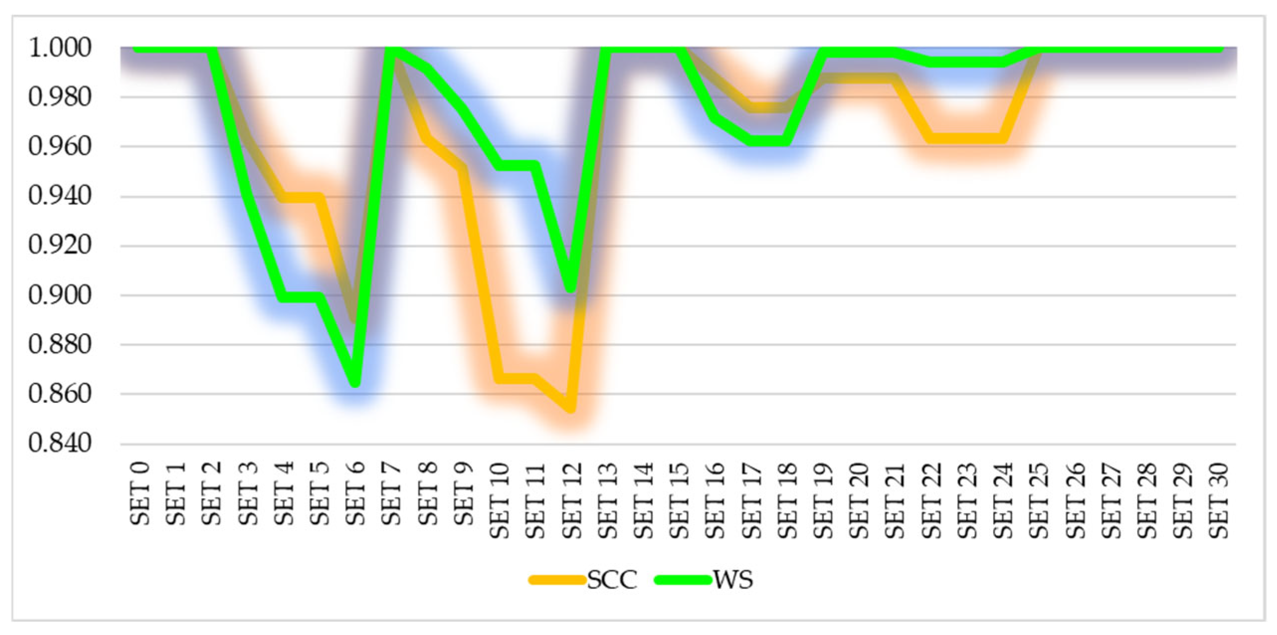
In the following section, a statistical test of correlation was performed to examine the consistency between the previously conducted tests. Two statistical correlation measures were calculated: SCC [61,62] and WS [63]. Regarding the comparative analysis, there is a perfect correlation between IRN AROMAN, IRN COCOSO, and IRN SAW, while the correlation with IRN COPRAS is slightly lower, with SCC = 0.952 and WS = 0.993.

Both statistical correlation coefficients reflecting the ranking changes during the sensitivity analysis are presented in Figure 6. The WS coefficient takes into account rank deviations. For example, if the best-placed variants have deviations, the WS coefficient will be smaller and will show a lower level of correlation, while if the deviations are closer to the last positions, the level of correlation will be higher. In general, the difference between the SCC and WS coefficients is, in fact, that the WS coefficient does not treat each difference in ranks.

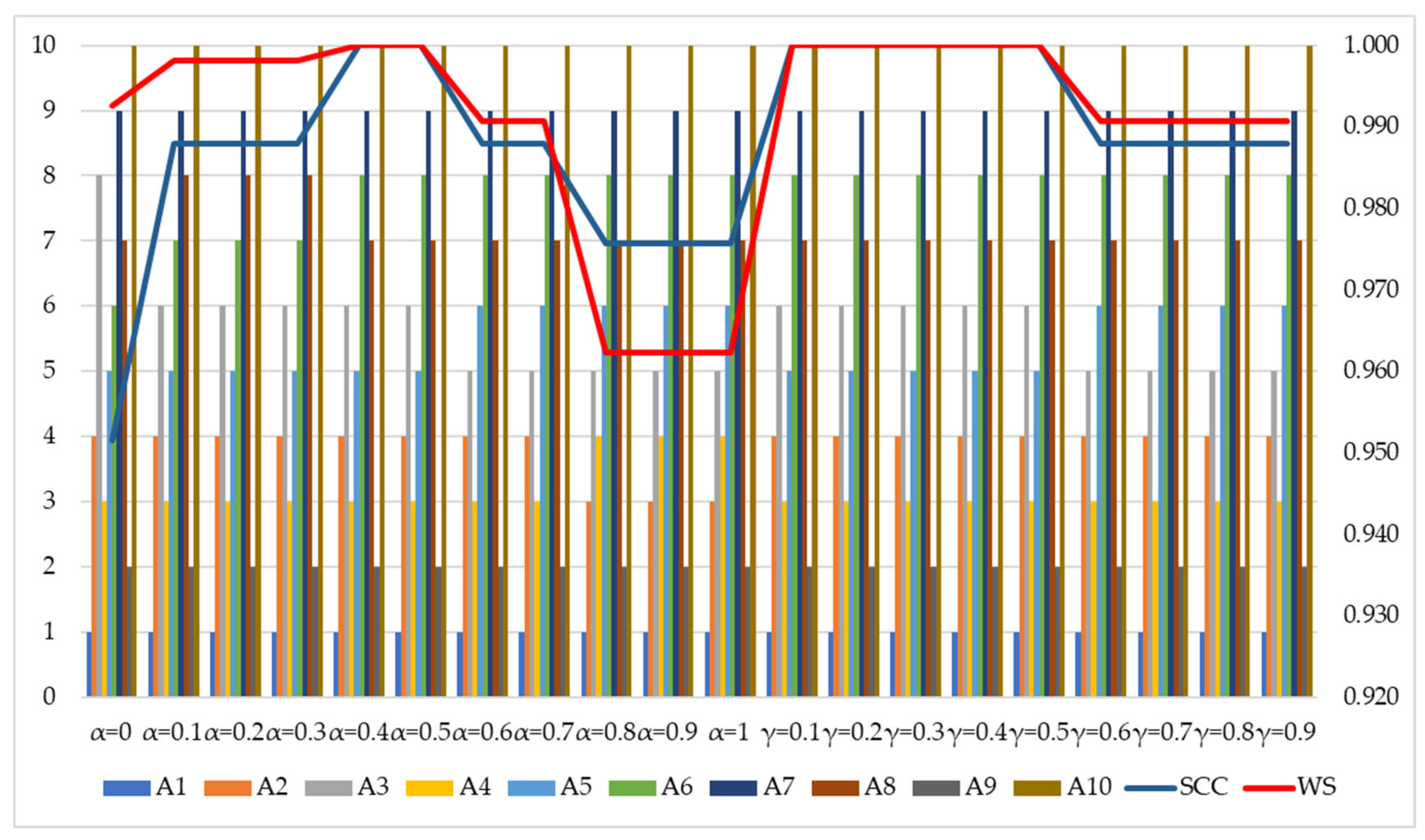
The statistical correlation coefficients show a very high average value, indicating a strong correlation in the sensitivity analysis. The average coefficients are as follows: SCC = 0.969 and WS = 0.976. The final test involves varying two coefficients, α and γ, in the IRN AROMAN method, which is illustrated in Figure 7.

Within the IRN AROMAN method, the value of coefficient α can range from 0 to 1, while coefficient γ ranges from 0.1 to 0.9. Under the standard application conditions of the IRN AROMAN method, both coefficients are set to 0.50. The sensitivity of the rankings to changes in these coefficients was assessed by varying their values within the specified intervals. Values of α = 0.4 and α = 0.5 do not influence the original obtained ranks, while all other values of this coefficient make a different ranking of potential variants. For example, if the value of this coefficient is equal to zero, A3 will be in eighth position, while A6 will receive sixth place. Practically, these two variants replaced their ranks. If we model α to be in the interval 0.1–0.3, alternatives A6 and A8 will replace their positions. The least correlation of WS = 0.962 occurs in cases when α is going toward one, because we have four changes in ranks.

Coefficient γ in the 0.1–0.5 interval does not have any influence on the ranking variants, while in the 0.6–0.9 interval, it influences only A3 and A5, which replaced their positions (5 and 6). The consequence of such modelling can be explained by the fact that all criteria have been modelled as benefits in the transformation of IRN.

In the shown case, coefficient α has more influence on the stability of results than coefficient γ.

The two top-performing delivery zones remain in their positions, while several other alternatives exhibit only minor changes in rank.

6. Discussion and Conclusions

The primary objective of this study was to examine the issues surrounding delivery areas in postal services. This is particularly relevant due to the increasingly rapid growth of e-commerce. The challenge facing postal operators is how to divide the delivery territory into balanced delivery areas. Priority attention has been given to the issue of productivity, as one of the key indicators for both delivery areas and the couriers serving them.

Various activities are being undertaken to improve productivity, ranging from investing in more efficient equipment to standardizing service delivery processes. Standardization in the service sector typically takes the form of manuals or operational procedures that regulate the behavior of operators and aim to minimize errors among employees. This approach achieves increased efficiency and reduced costs.

A new approach has been developed to determine productivity, modifying the formula used by the national operator based on available time for delivery and collection of shipments. Specifically, according to the principle of fairness, it is necessary to determine how much time the courier actually has available to perform the activities required by the postal operator. In other words, the total working time needs to be reduced by the distance traveled, which is an unavoidable side effect of courier activities.

The question arises: can productivity alone comprehensively describe a specific delivery area? Productivity is certainly an important element, but it does not provide insights into other aspects. Therefore, based on available data, in addition to productivity, we proposed certain key performance indicators (KPIs) such as failure rate, number of shipments, distance travelled, and CO₂ emissions per shipment. These KPIs could provide a more complete picture regarding delivery areas and indicate the need for their reorganization.

This model can be further expanded to include variables that characterize the quality of service in contact with the recipient of the shipment, as well as the value of the shipment (since the impact and economic consequences are not the same if a shipment worth €5 or €50 is not delivered).

What immediately catches the eye are the very high values of productivity (with only one area falling below the hypothetical). This raises the question of how they achieve such high levels of productivity. For example, whether they deliver the parcel directly to the door or call the recipient to come to the delivery vehicle and collect the parcel (eliminating idle time on return trips and avoiding wasting parking spaces).

The result of such a situation is a constantly open position for a deliveryman, not only with the operator under consideration but with all relevant operators in the postal services market. The main causes of this situation are primarily the increased volume of shipments due to e-commerce and the high turnover of deliverymen due to inadequately defined delivery areas.

The observed key KPIs were considered from the perspective of the sustainable functioning of the postal system. This involves the division of urban areas into delivery areas to achieve an optimal level of operations, considering the specified spatial and traffic parameters. It was concluded that the observed postal operator does not operate under optimal conditions, but there is potential for improving the observed parameters.

A limitation of this study lies in the limited number of experts involved, which could affect the generalizability of the findings. Moreover, the region-specific nature of the data may challenge the applicability of the results to other geographic contexts.

Future research could consider integrating dynamic data—such as traffic congestion, weather conditions, and real-time delivery information—to enhance model accuracy. Furthermore, incorporating customer satisfaction metrics would offer deeper insight into last-mile delivery efficiency. Lastly, subsequent studies might explore the use of advanced machine learning and artificial intelligence techniques to optimize delivery area processes.

References

1. Ducret, R. Parcel deliveries and urban logistics: Changes and challenges in the courier express and parcel sector in Europe—The French case. Res. Transp. Bus Manag. 2014, 11, 15–22. [Google Scholar] [CrossRef]
2. Kim, W.; Wang, X.C. The adoption of alternative delivery locations in New York City: Who and how far? Transp. Res. A Policy Pract. 2022, 158, 127–140. [Google Scholar] [CrossRef]
3. Rogers, M. The Definition and Measurement of Productivity; Melbourne Institute of Applied Economic and Social Research: Melbourne, Australia, 1998; pp. 1–27. [Google Scholar]
4. Schreyer, P.; Pilat, D. Measuring productivity. OECD Econ. Stud. 2001, 33, 127–170. [Google Scholar]
5. Edwards, K.; Jensen, P.L. Design of systems for productivity and well-being. Appl. Ergon. 2014, 45, 26–32. [Google Scholar] [CrossRef]
6. Syverson, C. What determines productivity? J. Econ. Lit. 2011, 49, 326–365. [Google Scholar] [CrossRef]
7. Segarra-Blasco, A. Innovation and productivity in manufacturing and service firms in Catalonia: A regional approach. Econ. Innov. New Technol. 2010, 19, 233–258. [Google Scholar] [CrossRef]
8. Stiroh, K.J. What drives productivity growth? Econ. Policy Rev. 2001, 7, 37–59. [Google Scholar]
9. Dresch, A.; Collatto, D.C.; Lacerda, D.P. Theoretical understanding between competitiveness and productivity: Firm level. Ing. Compet. 2018, 20, 69–86. [Google Scholar] [CrossRef]
10. Davenport, T.H.; Short, J.E. The New Industrial Engineering: Information Technology and Business Process Redesign; MIT: Cambridge, MA, USA, 1990; pp. 1–31. [Google Scholar]
11. Basu, S.; Fernald, J. Why is productivity procyclical? Why do we care? In New Developments in Productivity Analysis; Hulten, C., Dean, E., Harper, M., Eds.; University of Chicago Press: Chicago, IL, USA, 2001; pp. 225–302. [Google Scholar]
12. Conway, P.; De Rosa, D.; Nicoletti, G.; Steiner, F. Regulation, Competition and Productivity Convergence. OECD Econ. Stud. 2006, 37, 39–76. [Google Scholar] [CrossRef]
13. Auer, R.; Fischer, A.M. The effect of low-wage import competition on US inflationary pressure. J. Monet. Econ. 2010, 57, 491–503. [Google Scholar] [CrossRef]
14. Schmenner, R.W.; Swink, M.L. On theory in operations management. J. Oper. Manag. 1998, 17, 97–113. [Google Scholar] [CrossRef]
15. Schmenner, R.W. Service businesses and productivity. Decis. Sci. 2004, 35, 333–347. [Google Scholar] [CrossRef]
16. Collewet, M.; Sauermann, J. Working hours and productivity. Labour. Econ. 2017, 47, 96–106. [Google Scholar] [CrossRef]
17. Feldstein, M.S. Specification of the labour input in the aggregate production function. Rev. Econ. Stud. 1967, 34, 375–386. [Google Scholar] [CrossRef]
18. Pencavel, J. The productivity of working hours. Econ. J. 2015, 125, 2052–2076. [Google Scholar] [CrossRef]
19. Kretschmer, T. Information and communication technologies and productivity growth: A survey of the literature. OECD Econ. Stud. 2012, 195, 1–27. [Google Scholar]
20. Singh, J. Performance productivity and quality of frontline employees in service organizations. J. Mark. 2000, 64, 15–34. [Google Scholar] [CrossRef]
21. Mangiaracina, R.; Perego, A.; Seghezzi, A.; Tumino, A. Innovative solutions to increase last-mile delivery efficiency in B2C e-commerce: A literature review. Int. J. Phys. Distr. Log. 2019, 49, 901–920. [Google Scholar] [CrossRef]
22. Mohammad, W.A.; Nazih Diab, Y.; Elomri, A.; Triki, C. Innovative solutions in last mile delivery: Concepts, practices, challenges, and future directions. Supply Chain. Forum Int. J. 2023, 24, 151–169. [Google Scholar] [CrossRef]
23. Sorooshian, S.; Khademi Sharifabad, S.; Parsaee, M.; Afshari, A.R. Toward a modern last-mile delivery: Consequences and obstacles of intelligent technology. Appl. Syst. Innov. 2022, 5, 82. [Google Scholar] [CrossRef]
24. Stojčić, M.; Zavadskas, E.K.; Pamučar, D.; Stević, Ž.; Mardani, A. Application of MCDM methods in sustainability engineering: A literature review 2008–2018. Symmetry 2019, 11, 350. [Google Scholar] [CrossRef]
25. Krstić, M.; Tadić, S.; Kovač, M.; Roso, V.; Zečević, S. A novel hybrid MCDM model for the evaluation of sustainable last mile solutions. Math. Probl. Eng. 2021, 5969788. [Google Scholar] [CrossRef]
26. Tadić, S.; Krstić, M.; Radovanović, L. Assessing strategies to overcome barriers for drone usage in last-mile logistics: A novel hybrid fuzzy MCDM model. Mathematics 2024, 12, 367. [Google Scholar] [CrossRef]
27. Moslem, S.; Gündoğdu, F.K.; Saylam, S.; Pilla, F. A hybrid decomposed fuzzy multi-criteria decision-making model for optimizing parcel lockers location in the last-mile delivery landscape. Appl. Soft Comput. 2024, 154, 111321. [Google Scholar] [CrossRef]
28. Nur, F.; Alrahahleh, A.; Burch, R.; Babski-Reeves, K.; Marufuzzaman, M. Last mile delivery drone selection and evaluation using the interval-valued inferential fuzzy TOPSIS. J. Comput. Des. Eng. 2020, 7, 397–411. [Google Scholar] [CrossRef]
29. Li, Y.; Liu, X.; Chen, Y. Selection of logistics center location using Axiomatic Fuzzy Set and TOPSIS methodology in logistics management. Expert Syst. Appl. 2011, 38, 7901–7908. [Google Scholar] [CrossRef]
30. Stević, Ž.; Huskanović, E. Management of last-mile delivery through the selection of locations for parcel lockers. In Proceedings of the XXI International May Conference on Strategic Management–IMCSM25, Bor Lake, Serbia, 30 May 2025; pp. 1–11. [Google Scholar] [CrossRef]
31. Jacobs, R. Alternative methods to examine hospital efficiency: Data envelopment analysis and stochastic frontier analysis. Health Care Manag. Sci. 2001, 4, 103–115. [Google Scholar] [CrossRef]
32. Dar, A.H.; Mathur, S.K.; Mishra, S. The efficiency of Indian banks: A DEA, Malmquist and SFA analysis with bad output. J. Quant. Econ. 2021, 19, 653–701. [Google Scholar] [CrossRef]
33. Cullinane, K.; Wang, T.F.; Song, D.W.; Ji, P. The technical efficiency of container ports: Comparing data envelopment analysis and stochastic frontier analysis. Transp. Res. A Policy. Pract. 2006, 40, 354–374. [Google Scholar] [CrossRef]
34. Adler, N.; Friedman, L.; Sinuany-Stern, Z. Review of ranking methods in the data envelopment analysis context. Eur. J. Oper. Res. 2002, 140, 249–265. [Google Scholar] [CrossRef]
35. Post, T. Estimating non-convex production sets–imposing convex input sets and output sets in data envelopment analysis. Eur. J. Oper. Res. 2001, 131, 132–142. [Google Scholar] [CrossRef]
36. Newhouse, J.P. Frontier estimation: How useful a tool for health economics? J. Health Econ. 1994, 13, 317–322. [Google Scholar] [CrossRef] [PubMed]
37. Amornkitvikai, Y.; Harvie, C. Finance, ownership, executive remuneration, and technical efficiency: A stochastic frontier analysis (SFA) of Thai listed manufacturing enterprises. Austral. Account. Bu. 2011, 5, 35–55. [Google Scholar]
38. Mandil, A.D.A.; Salih, M.M.; Muhsen, Y.R. Opinion weight criteria method (OWCM): A new method for weighting criteria with zero inconsistency. IEEE Access 2024, 12, 5605–5616. [Google Scholar] [CrossRef]
39. Tanackov, I.; Badi, I.; Stević, Ž.; Pamučar, D.; Zavadskas, E.K.; Bausys, R. A novel hybrid interval rough SWARA–interval rough ARAS model for evaluation strategies of cleaner production. Sustainability 2022, 14, 4343. [Google Scholar] [CrossRef]
40. Song, M.; Stević, Ž.; Badi, I.; Marinković, D.; Lv, Y.; Zhong, K. Assessing public acceptance of autonomous vehicles using a novel IRN PIPRECIA-IRN AROMAN model. Facta Univ. Ser. Mech. Eng. 2025, 23, 127–145. [Google Scholar] [CrossRef]
41. Grönroos, C.; Ojasalo, K. Service productivity: Towards a conceptualization of the transformation of inputs into economic results in services. J. Bus. Res. 2004, 57, 414–423. [Google Scholar] [CrossRef]
42. Ojasalo, K.P. Conceptualizing Productivity in Services; Swedish School of Economics and Business Administration: Helsinki, Sweden, 1999. [Google Scholar]
43. Attar, A.A.; Gupta, A.K.; Desai, D.B. A study of various factors affecting labour productivity and methods to improve it. IOSR Mech. Civ. Eng. 2012, 1, 11–14. [Google Scholar]
44. Cleghorn, J.E. The productivity side of quality. Bus. Q. 1992, 57, 123–127. [Google Scholar]
45. PTT Glasnik 432 (In Serbian); Public Enterprise “Post of Serbia”: Belgrade, Serbia, 2006.
46. Wang, Y.; Zhang, D.; Liu, Q.; Shen, F.; Lee, L.H. Towards enhancing the last-mile delivery: An effective crowd-tasking model with scalable solutions. Transp. Res. E Logist. Transp. Rev. 2016, 93, 279–293. [Google Scholar] [CrossRef]
47. Rai, H.B.; Verlinde, S.; Macharis, C. Unlocking the failed delivery problem? Opportunities and challenges for smart locks from a consumer perspective. Res. Transp. Econ. 2021, 87, 100753. [Google Scholar] [CrossRef]
48. PostNord. E-Commerce in Europe 2021. Available online: https://www.postnord.se/siteassets/pdf/rapporter/e-commerce-in-europe-2021.pdf (accessed on 2 April 2024).
49. Mangiaracina, R.; Song, G.; Perego, A. Distribution network design: A literature review and a research agenda. Int. J. Phys. Distrib. Logist. Manag. 2015, 45, 506–531. [Google Scholar] [CrossRef]
50. Sigala, M.; Mylonakis, J. Developing a data envelopment analysis model for measuring and isolating the impact of contextual factors on hotel productivity. Int. J. Bus Perform. Manag. 2005, 7, 174–190. [Google Scholar] [CrossRef]
51. Bowen, D.E.; Schneider, B. Services marketing and management: Implications for organizational behavior. Res. Organ. Behav. 1988, 10, 43–80. [Google Scholar]
52. Dobni, D. A marketing-relevant framework for understanding service worker productivity. J. Serv. Mark. 2004, 18, 303–317. [Google Scholar] [CrossRef]
53. Jaworski, B.J. Toward a theory of marketing control: Environmental context, control types, and consequences. J. Mark. 1988, 52, 23–39. [Google Scholar] [CrossRef]
54. Blumberg, D.F. Strategies for improving field service operations productivity and quality. Serv. Ind. J. 1994, 14, 262–277. [Google Scholar] [CrossRef]
55. Lim, S.F.; Wang, Q.; Webster, S. Do it right the first time: Vehicle routing with home delivery attempt predictors. Prod. Oper. Manag. 2023, 32, 1262–1284. [Google Scholar] [CrossRef]
56. Rao, S.; Rabinovich, E.; Raju, D. The role of physical distribution services as determinants of product returns in Internet retailing. J. Oper. Manag. 2014, 32, 295–312. [Google Scholar] [CrossRef]
57. Statista. Average Cost per Failed Delivery in 2020, by Country. Available online: https://www.statista.com/statistics/973182/last-mile-delivery-average-cost/ (accessed on 12 August 2023).
58. Song, L.; Cherrett, T.; McLeod, F.; Guan, W. Addressing the last mile problem: Transport impacts of collection and delivery points. Transp. Res. Rec. 2009, 2097, 9–18. [Google Scholar] [CrossRef]
59. Edwards, J.B.; McKinnon, A.C.; Cullinane, S.L. Carbon Auditing the ‘Last Mile’: Modelling the Environmental Impacts of Conventional and Online Non-Food Shopping; Green Logistics Report; Heriot-Watt University: Edinburgh, UK, 2009. [Google Scholar]
60. Boyer, K.K.; Prud’homme, A.M.; Chung, W. The last mile challenge: Evaluating the effects of customer density and delivery window patterns. J. Bus. Logist. 2009, 30, 185–201. [Google Scholar] [CrossRef]
61. Božanić, D.; Epler, I.; Puška, A.; Biswas, S.; Marinković, D.; Koprivica, S. Application of the DIBR II–rough MABAC decision-making model for ranking methods and techniques of lean organization systems management in the process of technical maintenance. Facta Univ. Ser. Mech. Eng. 2024, 22, 101–123. [Google Scholar] [CrossRef]
62. Mousavi, M.N.; Ghalehteimouri, K.J.; Alizadeh, I.S.; Bahramijaf, S.; Shamsoddini, A. The Impact of Urban Governance on Enhancing Resilience in Informal Settlements: A Case Study from Jafarabad, Kermanshah. J. Urban Dev. Manag. 2024, 3, 95–108. [Google Scholar] [CrossRef]
63. Więckowski, J.; Kizielewicz, B.; Shekhovtsov, A.; Sałabun, W. How Do the Criteria Affect Sustainable Supplier Evaluation?—A Case Study Using Multi-Criteria Decision Analysis Methods in a Fuzzy Environment. J. Eng. Manag. Syst. Eng. 2023, 2, 37–52. [Google Scholar] [CrossRef]
Figure 1. Positions of delivery areas.
Mathematics 13 02845 g001
Figure 2. Results of comparative analysis with correlation coefficients.
Mathematics 13 02845 g002
Figure 3. New simulated IRN values of criteria.
Mathematics 13 02845 g003
Figure 4. New ranks after performed sensitivity analysis.
Mathematics 13 02845 g004
Figure 5. Changes in ranks after performed SA.
Mathematics 13 02845 g005
Figure 6. SCC and WS in SA.
Mathematics 13 02845 g006
Figure 7. Ranking verification depending on coefficients α and γ and correlation coefficients.
Mathematics 13 02845 g007