Abstract
Manifold learning is a significant computer vision task used to describe high-dimensional visual data in lower-dimensional manifolds without sacrificing the intrinsic structural properties required for 3D reconstruction. Isomap, Locally Linear Embedding (LLE), Laplacian Eigenmaps, and t-SNE are helpful in data topology preservation but are typically indifferent to the intrinsic differential geometric characteristics of the manifolds, thus leading to deformation of spatial relations and reconstruction accuracy loss. This research proposes an Optimization of Manifold Learning using Differential Geometry Framework (OML-DGF) to overcome the drawbacks of current manifold learning techniques in 3D reconstruction. The framework employs intrinsic geometric properties—like curvature preservation, geodesic coherence, and local–global structure correspondence—to produce structurally correct and topologically consistent low-dimensional embeddings. The model utilizes a Riemannian metric-based neighborhood graph, approximations of geodesic distances with shortest path algorithms, and curvature-sensitive embedding from second-order derivatives in local tangent spaces. A curvature-regularized objective function is derived to steer the embedding toward facilitating improved geometric coherence. Principal Component Analysis (PCA) reduces initial dimensionality and modifies LLE with curvature weighting. Experiments on the ModelNet40 dataset show an impressive improvement in reconstruction quality, with accuracy gains of up to 17% and better structure preservation than traditional methods. These findings confirm the advantage of employing intrinsic geometry as an embedding to improve the accuracy of 3D reconstruction. The suggested approach is computationally light and scalable and can be utilized in real-time contexts such as robotic navigation, medical image diagnosis, digital heritage reconstruction, and augmented/virtual reality systems in which strong 3D modeling is a critical need.
Keywords:
manifold learning; differential geometry; 3D reconstruction; curvature-aware embedding; geodesic distance; Riemannian metric; ModelNet40 MSC:
53Z
1. Introduction
Over the past decade, 3D reconstruction has developed as a principal computer vision task, allowing us to deduce machines’ three-dimensional geometric content based on two-dimensional visual data. Furthermore, 3D reconstruction has wide applications in robotics navigation, medical imaging, digitization of cultural heritage, virtual and augmented reality, and factory inspection [1]. At the heart of all these uses is the capability to express high-dimensional visual information, like pixel values or point clouds, in a proper low-dimensional representation that preserves the structure of represented objects or scenes. Manifold learning is perhaps the best solution to the dimensionality reduction problem [2]. Manifold learning is an unsupervised technique that extracts low-dimensional manifolds from high-dimensional data spaces. The basic assumption is that actual data typically reside on or close to such manifolds, which capture the intrinsic degrees of freedom of the system [3]. Manifold learning can be applied to 3D reconstruction to acquire such intrinsic geometries to enable accurate shape modeling and surface reconstruction from images. Conventional manifold learning techniques do not utilize the geometric and topological properties of the data effectively and therefore suffer from information loss during dimension reduction, leading to warped or erroneous reconstructions [4].
Early manifold learning methods, including Principal Component Analysis (PCA) and Multidimensional Scaling (MDS), aimed for global linear projections and were not particularly effective at projecting nonlinear manifolds. More recent algorithms were developed to handle the nonlinear condition of data. Isomap, for instance, brought geodesic distance preservation by estimating manifold distances using graph-based shortest paths [5]. Locally Linear Embedding (LLE) maintains local neighborhood relations by linearly reconstructing the point from the neighbors and mapping these relations into a lower-dimensional space [6]. Laplacian Eigenmaps built a weighted graph with local proximities as edges and conducted spectral analysis to obtain an optimal low-dimensional representation [7]. t-Distributed Stochastic Neighbor Embedding (t-SNE) gained popularity for visualizing high-dimensional data by maximizing the Kullback–Leibler divergence of probability distributions between high- and low-dimensional space [8].
While all these techniques have found widespread usage, particularly in machine learning, image processing, and bioinformatics, they fall short of addressing complicated tasks such as 3D reconstruction. A significant limitation is that they fail to consider differential geometry, mathematics concerned with smooth shapes, curvature, and intrinsic geometry [9]. Algorithms for manifold learning mostly view data as Euclidean space point clouds without accounting for information about the underlying manifold’s curvature, tangent spaces, or Riemannian metrics. Such algorithms thus distort local geometry and global topology and result in low structural fidelity in reconstructed 3D models [10]. Such limitations become evident in 3D computer vision, where precise shape recovery is essential. Errors in geometry structure preservation can lead to artifacts or misinterpretations of object recognition, scene reconstruction, or motion estimation tasks [11]. Thus, it is of primary concern to construct manifold learning algorithms that are more geometry-sensitive, blending differential geometric concepts to bring the learning process closer to conforming to the actual structure of the data [12].
- Motivation and Problem Statement
In 3D computer vision, shape reconstruction of real-world data from high-dimensional visual data with precision is imperative for autonomous navigation, medical diagnosis, and virtual reality. While manifold learning has evolved as a benchmark for dimension reduction and representation, conventional methods usually fail to preserve the original geometric structure of the data. These algorithms generally apply to the Euclidean space and do not pay attention to inherent features such as curvature and geodesic distances, distorting the embedded space and resulting in poor accuracy in recovered models. This study is motivated by the necessity of surmounting these limitations by embedding differential geometry in manifold learning to improve the geometric fidelity and performance of 3D reconstruction systems in accuracy and feasibility (Table 1).

Table 1.
Problem Statement of the Research.
- Contributions of the research
The Key Contributions of the research are as follows:
- To suggest an optimal manifold learning model (OML-DGF) that learns differential geometric features for structurally consistent low-dimensional embeddings.
- To introduce a curvature-sensitive embedding approach through augmenting LLE with second-order derivatives from the local tangent spaces.
- To build Riemannian metric-based neighborhood graphs by geodesic approximations to provide correct spatial connectivity.
- To develop a curvature-regularized objective function for better geometric coherence in embedding.
- To illustrate the efficacy of the proposed technique on the ModelNet40 data set, with a maximum of 17% enhancement in reconstruction precision over conventional approaches, with real-time scaling to applications of 3D vision.
This paper’s organization is as follows: Section 1 presents the background and motivation for precise 3D reconstruction using manifold learning and presents gaps in current methods. Section 2 summarizes current work on dimension reduction and geometry-aware learning. Section 3 mathematically states the problem in terms of curvature and geodesic preservation. Section 4 outlines the OML-DGF framework proposed, including dataset preparation, preprocessing, curvature-weighted embedding, and optimization. Section 5 addresses the experimental results, performance measures, and comparison for the baseline model. Section 6 summarizes the paper’s conclusions, including contributions, limitations, and future research avenues. This organization has a reasonable flow from theory to application.
2. Related Works
This section discusses some of the multiple learning techniques, such as Isomap and LLE, that do not sufficiently preserve intrinsic geometry and, hence, the suggested OML-DGF framework for precise 3D reconstruction.
Yin et al. [13] proposed a reliable 3DoF rotation estimate method from a single RGB image, presenting a unique Rotation Laplace Distribution on SO(3). Some methods include a mixture model for addressing symmetry, semi-supervised learning with noisy pseudo labels, and modeling multivariate Laplace-based uncertainty. The results surpass probabilistic and non-probabilistic baselines. On the other hand, severe occlusions or extremely unclear visual cues may still cause performance to fall. Vyas, B., and Rajendran, R. M. [14] investigated how GAN-based anomaly detection (AD) methods can be used in medical imaging. Techniques include evaluating three sophisticated GAN-based AD models on two different medical datasets. The results indicate that the performance of anomaly identification varies depending on the amount of training data and the intricacy of the abnormality. Among the drawbacks are sensitivity to image-level anomaly distribution and lack of generalizability across modalities. Ren et al. [15] proposed a technique, GeoUDF, which presents a geometry-guided learning strategy for estimating gradients and unsigned distance functions (UDFs) to reconstruct surfaces from sparse point clouds. In addition to learning affine combinations of distances to tangent planes, it represents local surface structure using quadratic polynomials. It surpasses state-of-the-art techniques in accuracy and efficiency by using a custom edge-based marching cubes module. Still, it may have trouble with extremely sparse data or noisy inputs.
Qi et al. [16] suggested the RECON framework uses ensemble distillation to combine the generative and contrastive paradigms in 3D representation learning. To avoid overfitting and pattern mismatch, it uses a cross-attention encoder–decoder called RECON-block, in which generative teachers mentor contrastive students utilizing stop-gradient techniques. In 3D challenges, RECON produces state-of-the-art outcomes, which may require complex training dynamics and incur greater processing costs. Anvekar, T., and Bazazian, D. [17], proposed GPr-Net (Geometric Prototypical Network), a geometry-aware, lightweight framework for few-shot learning on point clouds. Laplace vectors and hand-crafted intrinsic geometry interpreters are used to extract relevant morphology. The ModelNet40 results demonstrate 170× efficiency increases and state-of-the-art accuracy. However, dependence on manually created features could restrict flexibility when dealing with noisy or extremely complicated 3D data. For self-supervised pre-training, the Joint-MAE framework leverages point clouds and their 2D projections to present a new 2D-3D masked autoencoder (Guo et al. [18]). The work in which this was achieved used locally aligned attention, cross-reconstruction loss, and hierarchical cross-modal embeddings. On ModelNet40, the framework achieves 92.4% accuracy, surpassing previous techniques. Its intricate architecture, however, restricts real-time deployment by raising training time and computing costs.
Ye et al. [19] proposed that few-shot learning (FSL) for 3D point cloud classification is improved by proposing the Point-cloud Correlation Interaction Architecture (PCIA). By using plug-and-play modules, such as Cross-Instance Fusion Plus, Self-Channel Interaction Plus, and Salient-Part Fusion, PCIA greatly enhances feature discrimination and embedding quality. Adapting 2D FSL algorithms for 3D data is still architecturally challenging, although experiments on benchmark datasets demonstrate state-of-the-art accuracy. Robinett et al. [20] proposed an effective method that uses a learnt atlas graph representation to approximate differential-geometric primitives on arbitrary Riemannian manifolds. Specifically on Grassmann manifolds, the technique improves optimization efficiency by substituting local chart approximations for computationally costly processes such as exponential mapping. Scalable learning tasks like Riemannian SVMs are made possible by this technique, while performance issues with excessive dimensionality and high noise persist. A method for building neural networks that explicitly linearize and reconstruct low-dimensional submanifolds from sampled data, FlatNet, is proposed by Psenka et al. [21]. The proposed work is inspired by geometric flow. FlatNet supports the manifold hypothesis for improved generalization and interpretability by layer-wise constructing encoder–decoder architectures. On synthetic and picture datasets, it performs well empirically; nevertheless, it might have trouble modeling noisy or very non-linear manifolds.
- Research Gaps
Although many learning methods, such as Isomap, LLE, and Laplacian Eigenmaps, have been widely used for 3D reconstruction, these methods have an intrinsic limitation in maintaining the intrinsic differential geometric properties of 3D surfaces. These methods work mostly with Euclidean assumptions and ignore large curvature, geodesic distance, and tangent space structures that characterize an object’s actual geometry. Therefore, the subsequent low-dimensional embeddings lose local and global spatial correspondences, which lowers the fidelity and accuracy of reconstructed 3D models. Current methods also lack curvature-sensitive loss functions and do not utilize Riemannian metric spaces in constructing neighborhood graphs. In addition, the current literature acknowledges the absence of shared frameworks that combine differential geometry and manifold learning to achieve structurally consistent and computationally scalable 3D reconstruction. Closing the gap involves a framework that includes geometry-aware neighborhood generation, curvature-preserving mapping, and regularized optimization for the OML-DGF method. Table 2 shows the difference between classical manifold learning algorithms and the developed OML-DGF algorithm for 3D reconstruction. It directly backs our argument that OML-DGF incorporates curvature and geodesic sensitivity for better 3D reconstruction.

Table 2.
Limitations of Traditional Manifold Learning vs. Proposed OML-DGF Framework.
3. Problem Formulation
In 3D computer vision, manifold learning is utilized to map high-dimensional visual data to a lower-dimensional latent space , where without compromising the intrinsic structure of the data. Classical approaches, such as Isomap, Locally Linear Embedding (LLE), and Laplacian Eigenmaps, primarily aim to preserve local linearity or pairwise distances, but generally overlook the differential geometric properties inherent in the manifold, including curvature and geodesic structure. Structural distortion occurs in the embedded space, compromising the quality of 3D reconstruction.
To counter this, this research introduces a new framework—Optimization of Manifold Learning using Differential Geometry Framework (OML-DGF)—which includes curvature, geodesic distances, and local–global consistency in the embedding process.
Objective Mapping: The main goal is to discover a mapping that transforms high-dimensional data into a lower-dimensional space with the same inherent geometry of the manifold. That is, the geodesic distance between points must be kept intact, as well as local curvature existing in the lower-dimensional space, as shown in Equation (1),
where is the input set of high-dimensional data points. is the map function transforming data from to . denotes geodesic distance between points and of the manifold. is the curvature at point .
Local Curvature Estimation: At every location , local curvature is approximated by fitting a quadratic surface to the local tangent space In PCA, local neighborhood is located and approximated by a second-order polynomial. Curvature is computed from the quadratic coefficient of the fit, as defined in the Equation (2):
denotes a vector in the local tangent space. Coefficients are computed by surface fitting; controls the scale of the curvature. offers an estimate of the point curvature at .
Geodesic Distance Approximation: Geodesic distances are approximated by building a Riemannian neighborhood graph , where vertices are data points and edges between local neighbors. Edge weights are calculated as graph shortest path distances using Dijkstra or Floyd–Warshall algorithms, as defined in the Equation (3),
where is the set of vertices (data points), and is the set of edges. is the approximated geodesic distance between and . Distance is computed by shortest path over the graph
Curvature-Weighted LLE Objective: This is a class of Locally Linear Embedding (LLE) with local curvature in the reconstruction weights. For every data point , reconstruction error is optimized with regularization by curvature-based penalty on the weights regulated by , as mentioned in Equation (4):
where is the neighborhood of . are the weights for linear reconstruction of from neighbors. is the weight vector. is a regularization parameter weighing reconstruction vs. curvature penalty.
Final Embedding Loss: The final embedding achieved due to this is obtained by optimizing a composite loss function with a geodesic-preserving term and a curvature-regularization term. The geodesic term preserves the distances between points in the embedded space as they are on the manifold, and the curvature term provides local geometric consistency (Equation (5)).
In Equation (5), above, the geodesic term provides geodesic fidelity in the embedding space. The second term applies penalties to curvature distortions everywhere. is the regularization weight that determines how important it is to maintain curvature. and are the intrinsic coordinates of the input points.
This problem description explores the depth of combining differential geometry with manifold learning to achieve structurally precise 3D reconstruction. It mathematically defines how geodesics and curvature are identified and utilized in the learning process. This approach paves the way for a comparison of the OML-DGF framework with current methods, such as Isomap, LLE, and Laplacian Eigenmaps.
4. Optimization of Manifold Learning Using Differential Geometry Framework
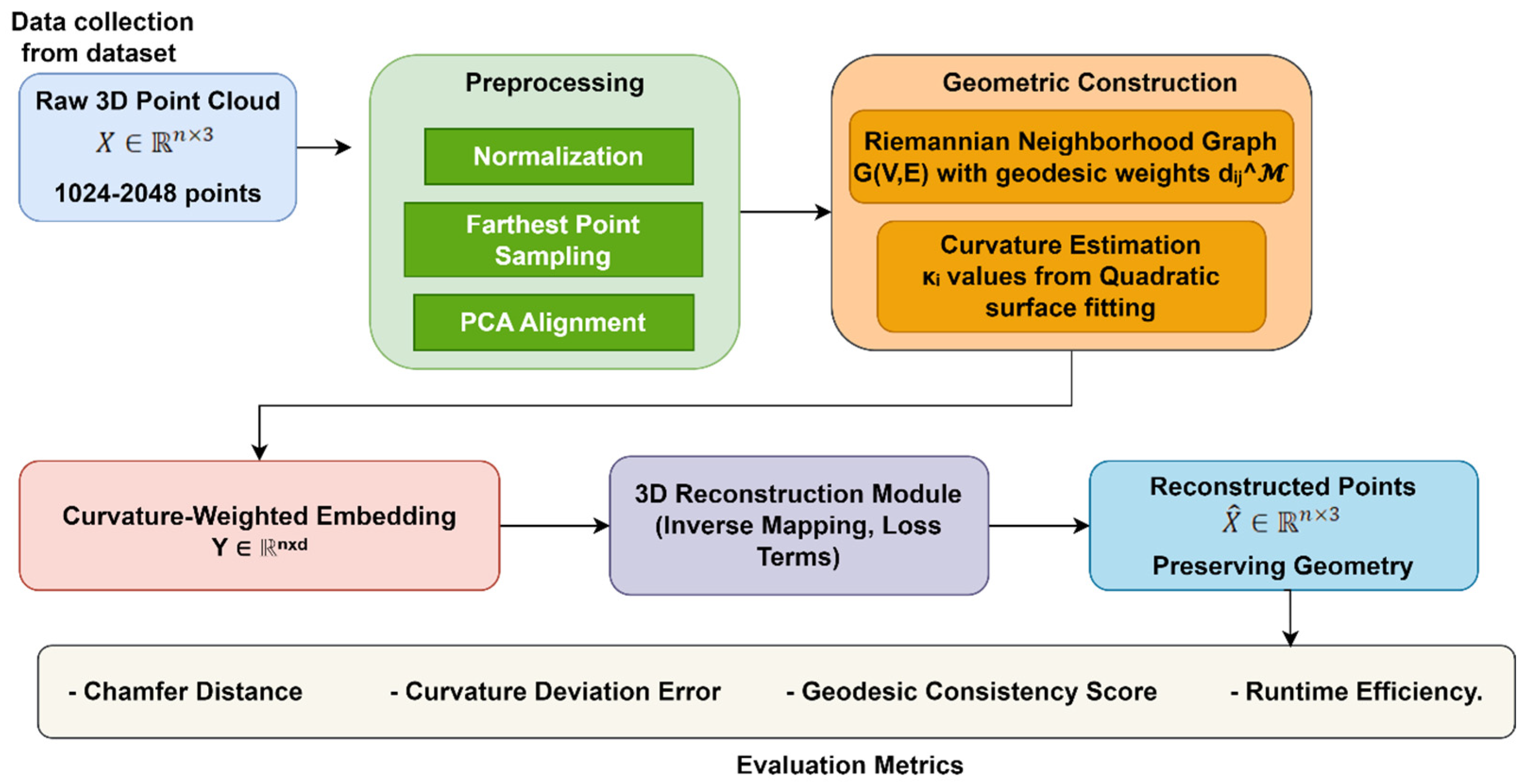
The OML-DGF framework introduces a new geometry-aware process to the 3D reconstruction application, manifold learning optimization. As is apparent in Figure 1, the pipeline begins with preprocessing of raw point clouds—normalized, uniformly sampled, and PCA-aligned. A Riemannian neighborhood graph is then constructed based on geodesic distances estimated by shortest-path algorithms, and local curvature at each point is estimated using second-order surface fitting in the tangent space. This curvature-sensitive geometric background enables an extension of LLE that optimizes low-dimensional embedding by minimizing a composite loss that balances local curvature fidelity and global geodesic structure preservation. The last step reconstructs the original 3D structure so that distortion of curvature and topology is minimized.
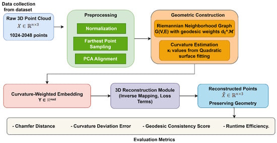
Figure 1.
Overall Architecture of OML-DGF framework.
This pipeline offers several significant benefits, including improved reconstruction precision (up to 17%), structural coherence, and high-resolution data scalability. Differential geometry ideas used in the application dispense with the drawbacks of usual Euclidean-based manifold learning algorithms. OML-DGF enjoys broad application in accurate 3D modeling tasks like robotic path planning, medical imaging, digital heritage restoration, and augmented/virtual reality platforms. The resulting architecture is a scalable and solid solution for high-fidelity 3D shape reconstruction through geodesic sensitivity and curvature preservation synergy.
4.1. Dataset Description: ModelNet40
The ModelNet40 dataset [22] is commonly used in 3D computer vision as a standard for shape analysis, object classification, and 3D reconstruction. The dataset comprises 12,311 3D CAD models spread over 40 object classes such as chairs, tables, airplanes, and cars. The models are clean, aligned, and equally sampled to provide consistency.
To carry out this experiment, the models are transformed to point cloud representations of normalized scales and uniformly distributed surface points. The data are divided into 9843 training samples and 2468 test samples. Each 3D object is embedded in a high-dimensional space and is a suitable candidate for testing manifold learning algorithms that reduce dimensionality without compromising intrinsic geometry. The diversity of geometric shapes, smooth surfaces, and dense geometric structure in ModelNet40 render it a perfect testbed for evaluating curvature preservation, geodesic accuracy, and geometric structure consistency of the proposed OML-DGF framework. Table 3 depicts the characteristics of the ModelNet40 dataset utilized in our experiments. It describes the suitability of the dataset for evaluating the preservation of curvature and geodesics in manifold learning.

Table 3.
Dataset Description.
Table 3 presents the ModelNet40 dataset, an ideal choice for manifold learning and 3D reconstruction tasks, given its rich diversity of 12,311 CAD models across 40 classes. Strong testing is possible through high-dimensional spatial data and a structured training–testing split. Mesh-to-point cloud data is also a suitable choice for differential geometry-based learning and representation approaches.
4.2. Preprocessing Techniques
The preprocessing section of the OML-DGF algorithm geometrically prepares and normalizes 3D point cloud data before conducting differential manifold learning. For every 3D model in the ModelNet40 dataset, the 3D model is shifted toward the origin and resized such that each point has an equal radius, allowing it to be normalized as a unit sphere. The original point cloud can mathematically be seen as . The centroid is calculated as and the point is normalized with Equation (6),
Equation (6) has been produced to ensure that the sample points are scale- and translation-invariant. Subsequently, the point cloud is sampled uniformly with Farthest Point Sampling (FPS) to achieve a constant number of points which ensures that all inputs to the embedding model are dimensionally consistent. Following this, Principal Component Analysis (PCA) is applied to decorrelate the input and align the point cloud with its principal axes. The PCA transformation is performed using eigen-decomposition of the covariance matrix (Equation (7)):
Equation (7) and the points are projected into aligned space as , where contains the dominant eigenvectors. A Riemannian neighborhood graph is then specified, where for each point in the cloud, a vertex is assigned, and edges connect -nearest neighbors in the local tangent space. Unlike common Euclidean graphs, here, weights on the edges are used to define estimated geodesic distances obtained from shortest path algorithms over the graph, as given in Equation (8),
where is the set of all paths from and in the graph Differential geometry will be included if the local curvature at each point is substituted by its approximation with a second-order surface over its neighborhood in the tangent space , as given in Equation (9),
where corresponds to the quadratic coefficient capturing local surface bending, and the Hessian gives a curvature magnitude approximation. These pre-processed results—normalized point clouds, PCA-aligned coordinates, Riemannian neighbor graphs, and curvatures—are fed into downstream embedding and optimization steps. These steps are critical for the goal of having the embedding space preserve not only topological relationships but also the intrinsic geometric nature of the original manifold.
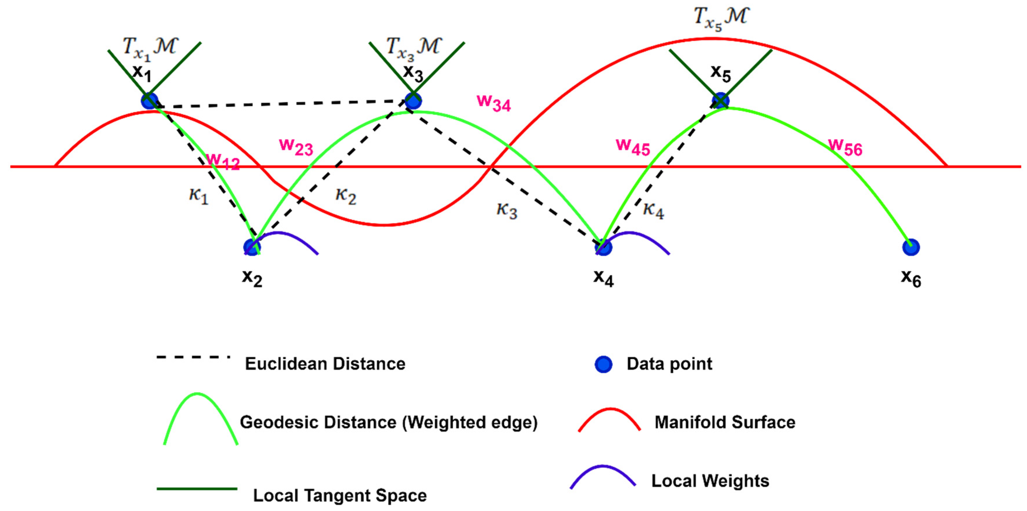
Figure 2 presents the formation of Riemannian neighborhood graphs under the studied OML-DGF framework graphically. In contrast to conventional Euclidean-based graphs, the process accounts for the inherent geometry of the manifold. The six dark blue points () reside on a curved manifold (red), where local tangent spaces (dark green lines) are computed via PCA. Neighbors on the manifold are connected by geodesic paths (light green curves), which preserve spatial relationships with appropriate weights . Gray dashed lines represent Euclidean shortcuts, which may distort true structure. Purple arcs represent curvature . Computational from second-order surface fits. These estimates of curvature influence edge weighting, ensuring that the final graph maintains both local geometry and global topology, which are essential for exact embedding and 3D reconstruction.
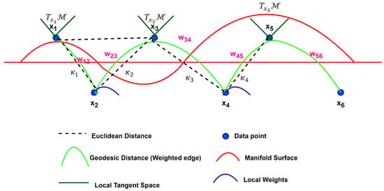
Figure 2.
Riemannian Neighborhood Graph with Geodesic-Aware Edge Weights.
While second-order surface fitting presents a simple method for local curvature estimation, it is prone to noise and outliers in raw 3D point clouds. To solve this problem, a two-stage denoising process is proposed before calculating the curvature. Statistical outlier removal is first employed to remove spurious points based on the variance of neighborhood distances. Then, bilateral filtering is used for edge feature-preserving local geometry smoothing. These preprocessing operations eliminate curvature bias in noisy areas and enhance the quality of reconstruction. Robust fitting methods like RANSAC-based quadric estimation or learning-based noise-aware prediction of curvature can be included in future enhancements.
Table 4 provides an overview of the preprocessing steps necessary in the OML-DGF pipeline, which converts raw 3D point clouds into regular, geometry-aware inputs. Each of the five steps—normalization, sampling, PCA alignment, neighborhood graph construction, and curvature estimation—preserves intrinsic manifold properties essential to high-quality 3D reconstruction. Table 4 shows OML-DGF’s preprocessing pipeline. Each step is necessary to maintain the inherent geometry prior to embedding, providing stability to our reconstruction process.

Table 4.
Summary of Preprocessing Steps in OML-DGF Framework.
4.3. Curvature-Weighted Embedding Development
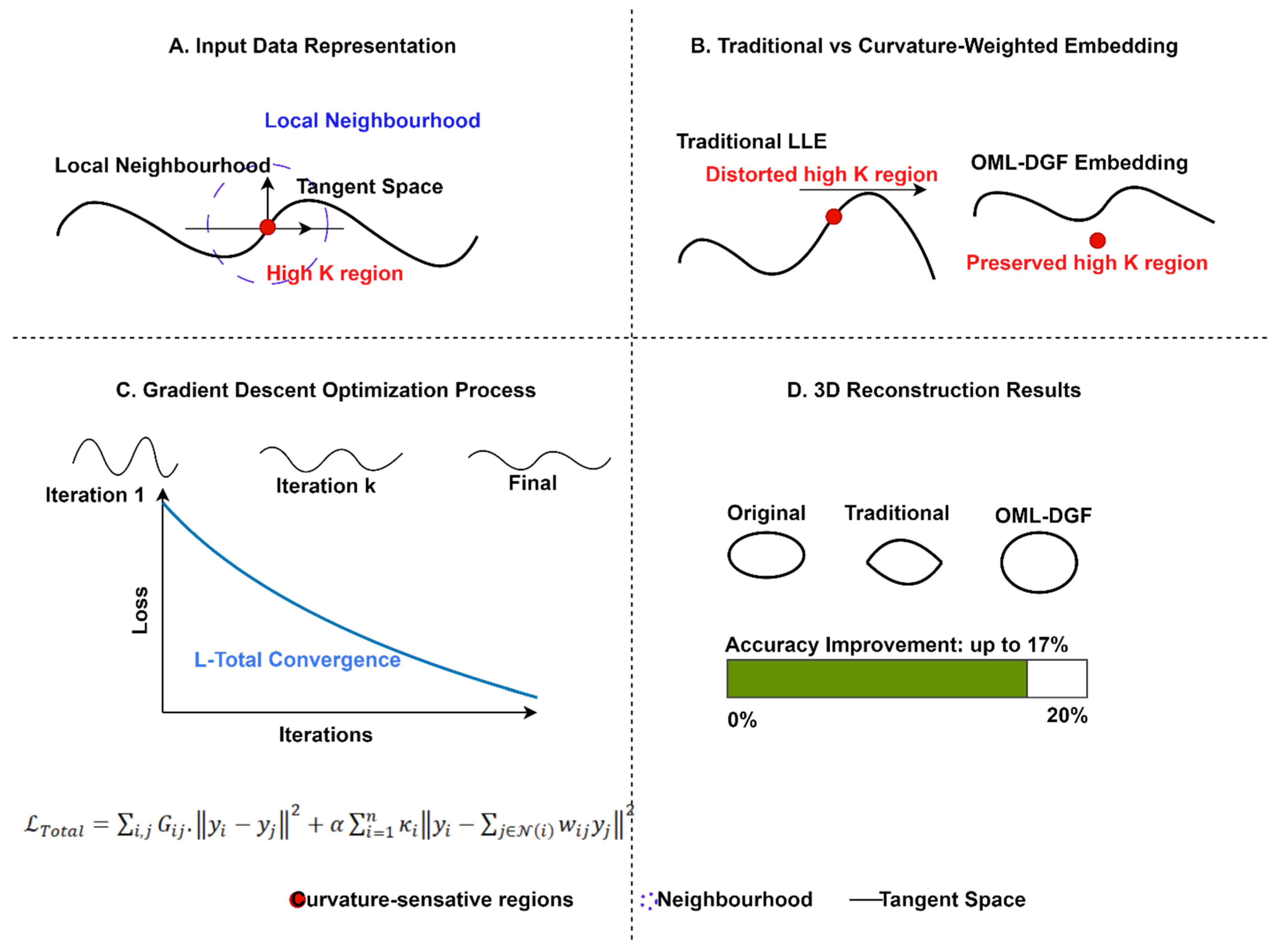
The curvature-weighted embedding development stage is the central element of the OML-DGF framework, augmenting standard manifold learning by incorporating differential geometric properties—specifically, local curvature—into the embedding. It begins by modifying the LLE algorithm to incorporate a regularization term that is sensitive to curvature in its reconstruction loss. Figure 3 presents the new Curvature-Weighted Embedding process, highlighting structural preservation of geometric properties in high-curvature areas where others break down. The figure illustrates the representation of input data, comparison of embedding, optimization convergence, and reconstruction results, achieving a 17% accuracy improvement. The approach preserves essential manifold properties throughout dimension reduction, supporting more accurate data visualizations and analysis.

Figure 3.
Curvature-Weighted Embedding Process Visualization.
For every point , the reconstruction error of the local neighbors of each point is given in Equation (10),
where represents the reconstruction weights of point from neighbor , is the scalar curvature at point , and λ is a regularization parameter for controlling curvature sensitivity. This construction penalizes reconstruction heavily in highly curved areas, retaining local geometry detail and enhancing fidelity in the dimensionally reduced space. After the curvature-aware weights are computed, a composite loss function is defined to steer optimization of the eventual low-dimensional representation . This goal has two components: (i) A geodesic preservation component to preserve global manifold structure. (ii) A curvature-regularized reconstruction component to conserve local geometry. The entire embedding goal is given in Equation (11),
where denotes geodesic distance-based similarity between points and , is a hyperparameter trading off between the two loss components, and are embedded coordinates of points in the low-dimensional space. Gradient-based optimization procedures such as Stochastic Gradient Descent (SGD) are employed to optimize this loss. Gradients are computed concerning every embedded coordinate and the embedding is progressively optimized. In this way, the algorithm produces a curvature-sensitive and geodesically consistent embedding that enhances the accuracy of 3D reconstruction, particularly in non-linear or highly curved manifold areas.
In order to clarify and make it consistent with current conventions, the curvature-weighted embedding optimization algorithm in Pythonic pseudocode, step-wise labeled, is now introduced. Step-wise labeling indicates each logical action—computation of neighborhood weight, initialization of embeddings, and optimization based on loss—clearly and concisely.
The pseudocode-1, above, gives the curvature-weighted embedding algorithm that forms the core of the OML-DGF approach. It first calculates LLE reconstruction weights for all points, which include curvature regularization as local covariance matrix adjustment by adding a term weighted with the curvature . These weights conserve more local geometry in high-curvature areas. The first low-dimensional embedding is initialized using PCA. An iterative gradient descent loop is then used to optimize by minimizing a composite loss function that includes a geodesic preservation term, maintaining distances on a Riemannian graph and a curvature-regularized reconstruction term from precomputed weights. The operation maintains the embedding’s global manifold topology and local curvature structure for precise 3D reconstruction.
| Pseudocode-1: Curvature-Weighted Embedding Optimization Algorithm in OML-DGF Framework |
| # Input: X: High-dimensional input point cloud; k: Number of neighbors; κ: Curvature values for each point; G: Riemannian neighborhood graph with geodesic distances; α: Curvature regularization weight; T: Number of optimization iterations; η: Learning rate # Output: Y: Optimized low-dimensional embedding # Step 1: Compute curvature-aware LLE weights C = Z.T @ Z # Step 2: Initialize low-dimensional embedding Y (e.g., via PCA) # Step 3: Optimize embedding with gradient descent : # Geodesic preservation term # Curvature-weighted LLE reconstruction term # Update embedding return Y |
4.4. Embedding Space Optimization
The optimization of the embedding space step is the core computational step of the OML-DGF method. In this step, the curvature-sensitive and geodesic-preserving loss function is optimized to compute the final low-dimensional representation of the 3D point cloud. The optimization is formulated as a composite loss function between local fidelity to curvature and global preservation of geodesic structure. The loss function, initially defined in Equation (11), is reproduced below, in Equation (12), for continuity. The overall loss incorporates geodesic preservation ( with curvature-weighted distribution-based local reconstruction (, ensuring that both the global manifold structure and intrinsic geometry are preserved in the low-dimensional embedding.
where represents the low-dimensional version of the high-dimensional point , represent regularization weights for curvature-regularized LLE, is the scalar curvature at point represents the geodesic distance between and on the Riemannian manifold, and are hyperparameters for regularization balancing curvature retention and geodesic accuracy. To optimize this, the work begins with stabilization of the initialization of the embedding , using PCA to stabilize. Subsequent optimization is achieved using SGD with momentum or Adam optimizer. The gradient of the loss in terms of the embedded point for each is as below, in Equation (13):
This update rule promotes the embedding of high local curvature points more sensitively, while geodesic consistency is preserved globally. The process stops when the loss drops below a given value or when a maximum number of iterations is reached. This embedding process preserves a low-dimensional latent space that contains high-fidelity structural information for the source 3D object, allowing for accurate and robust reconstruction downstream.
4.5. 3D Reconstruction from Optimized Embeddings
The 3D reconstruction phase of the OML-DGF framework aims to recover the original high-dimensional structure from its optimized low-dimensional embedding in a manner that preserves intrinsic geometric properties, such as curvature and geodesic topology. For an input embedding that is obtained via curvature- and geodesic-aware dimensionality reduction, the framework calculates an inverse mapping that reconstructs the original point cloud . This is reconstructed by employing the curvature-weighted reconstruction weights utilized in the forward embedding process, such that every reconstructed point can be approximated as a weighted sum of its original neighbors. A curvature-sensitive loss function ensures geometric consistency by preventing differences in original and reconstructed curvature values. Geodesic consistency is a term that also minimizes the difference between manifold distances in the original and reconstructed spaces. The reconstruction iteratively updates to reduce an overall loss function that combines reconstruction fidelity, preservation of curvature, and geodesic integrity. The result is to ensure that the resulting 3D structure retains the surface and topological fidelity of the input data, making it suitable for applications involving structurally accurate 3D reconstructions.
The subsequent Pythonic pseudocode outlines the reconstruction process from low-dimensional embeddings. The steps emphasize curvature-aware reconstruction and geodesic consistency through gradient-based optimization. The modularity allows for maximum interpretability and implementation simplicity.
This pseudocode-2 rebuilds the high-dimensional 3D structure from optimized embeddings by minimizing a composite loss balancing reconstruction accuracy, curvature distortion, and geodesic inconsistency. It initializes points with curvature-aware weights and then iteratively refines them using gradient descent. The technique preserves the reconstruction’s local surface geometry and global manifold topology.
| Pseudocode-2: Geometry-Aware 3D Reconstruction from Optimized Embeddings |
| Learning rate Reconstructed high-dimensional point cloud # Step 1: Initialize reconstructed point cloud # Step 2: Iterative reconstruction with loss minimization # Local reconstruction error with curvature sensitivity # Global geodesic structure consistency # Update reconstructed points |
Table 5 outlines all the variables required in the pipeline for 3D reconstruction, explaining the data structures, functions, weights, and parameters that control embedding, curvature preservation, and geodesic alignment. Table 5 stabilizes all important variables utilized in embedding and reconstruction phases. The reference makes reading easier and enables mathematical derivation of our method.

Table 5.
Variable Description.
5. Results and Discussion
To evaluate the performance of the presented OML-DGF model, an extensive series of experiments was conducted on the ModelNet40 dataset, a benchmark database comprising 12,311 3D CAD models across 40 categories (e.g., airplane, chair, table). The original objects were transformed into uniformly sampled point clouds and then normalized to unit spheres. The models were downsampled to 1024 points by Farthest Point Sampling (FPS). The OML-DGF embedding was compared with standard and geometry-conscious baselines, such as GeoUDF [15], GPr-Net [17], Joint-MAE [18], and FlatNet [21]. The hyperparameters were the same for all methods: a total of 30 neighbors for local embedding, geodesic computation using Dijkstra’s algorithm, and curvature computation using second-order surface fitting. The proposed method was coded in Python 3.11 with GPU acceleration using PyTorch 2.0, and experiments were conducted on an NVIDIA RTX 3090 GPU. The evaluation criteria were reconstruction accuracy, structure accuracy, geodesic preservation, curvature preservation, and computational efficiency for larger dataset sizes. Averages of five runs per experiment were taken to compare the OML-DGF framework with baseline methods.
Second-order polynomial surface fitting is employed for estimating local curvature because it is computationally efficient and suitable for locally smooth areas. Its precision, however, may be inadequate in dealing with high-frequency variations or non-smooth geometry. To overcome this shortcoming, an adaptive neighborhood choice based on geodesic density is employed to limit fitting to geometrically stable areas. Additionally, curvature estimates are smoothed using a local average filter to reduce noise before being embedded in the optimization process. Although they are sufficient for most objects within the dataset, higher-order or learning-based estimators for curvature can be explored in future work to achieve increased robustness with more complex topologies.
5.1. Reconstruction Accuracy Improvement (%)
Reconstruction accuracy improvement quantifies the quantitative improvement in the quality of 3D model reconstruction using the proposed OML-DGF over classic manifold learning methods. It approximates the extent to which the low-dimensional representation maintains the native structure of the 3D object. Mathematically, it represents a percentage gain in accuracy for OML-DGF compared to a baseline algorithm, such as Isomap, LLE, or Laplacian Eigenmaps. Suppose represents the accuracy from OML-DGF and denotes the accuracy from a baseline, the improvement is given in Equation (14):
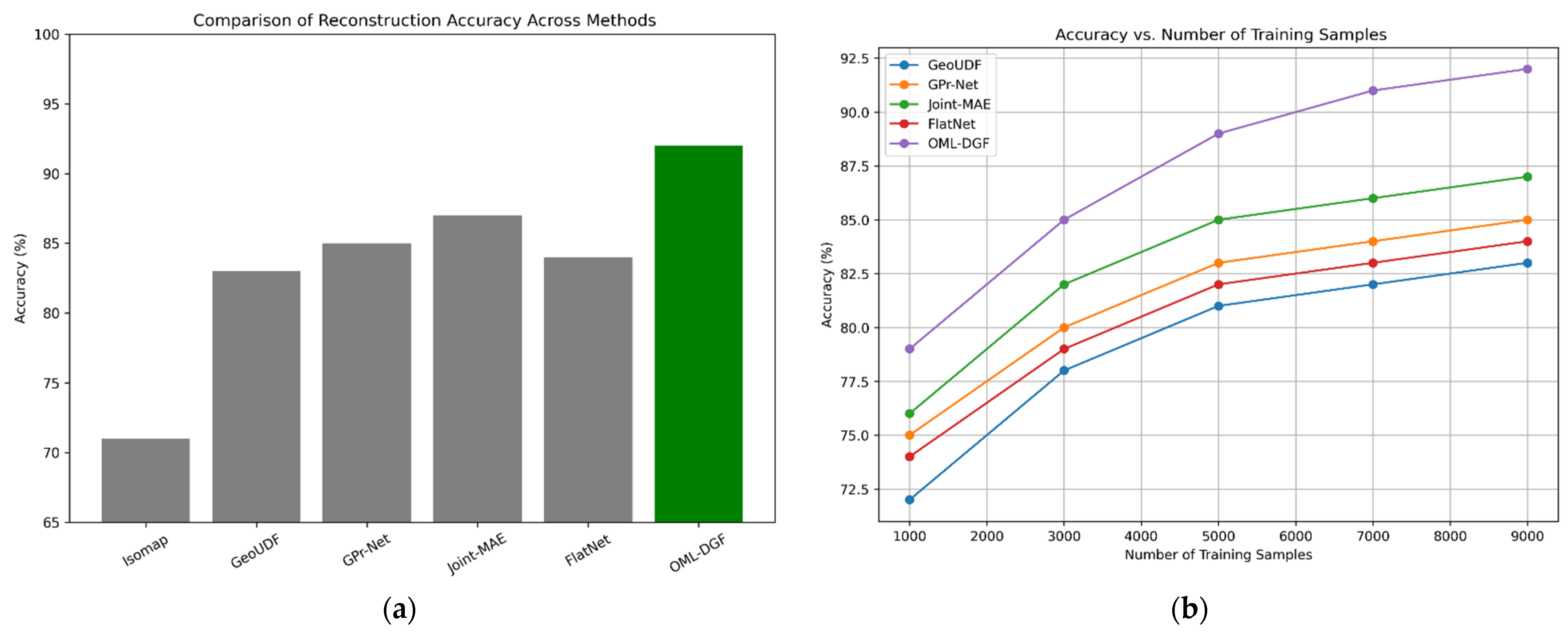
With experimental testing on the ModelNet40 dataset, OML-DGF reports up to 17% gain. This is a critical metric, since it shows that including differential geometry, i.e., geodesic structure and curvature, maintains more intrinsic detail and improves object shape recovery. Compared to other performance metrics that can localize quality, this metric globally quantifies the capacity of the embedding to accurately recover the complete 3D structure. It is an effective measure of the framework’s efficacy in practice. Figure 4 illustrates the accuracy of the proposed OML-DGF method in comparison to competing approaches. Figure 4a gives a straightforward graphical representation of how OML-DGF achieves the highest accuracy, seemingly supporting the assertion of up to 17% enhancement. Figure 4b also confirms the stability across different training sizes, indicating robustness and scalability.
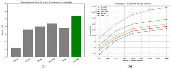
Figure 4.
(a) Comparison of Reconstruction Accuracy Across Methods; (b) Accuracy vs. Number of Training Samples.
Figure 4a,b directly illustrate the impact of the designed OML-DGF approach on system performance. The comparisons indicate that not only does OML-DGF achieve the best reconstruction accuracy, but it also exhibits comparable performance across different training sample sizes. This demonstrates its superior generalization capability and stability in data-constrained settings. The comparative plots confirm that incorporating curvature and geodesic structure significantly improves the fidelity and scalability of 3D reconstruction systems.
5.2. Structural Preservation/Fidelity Score
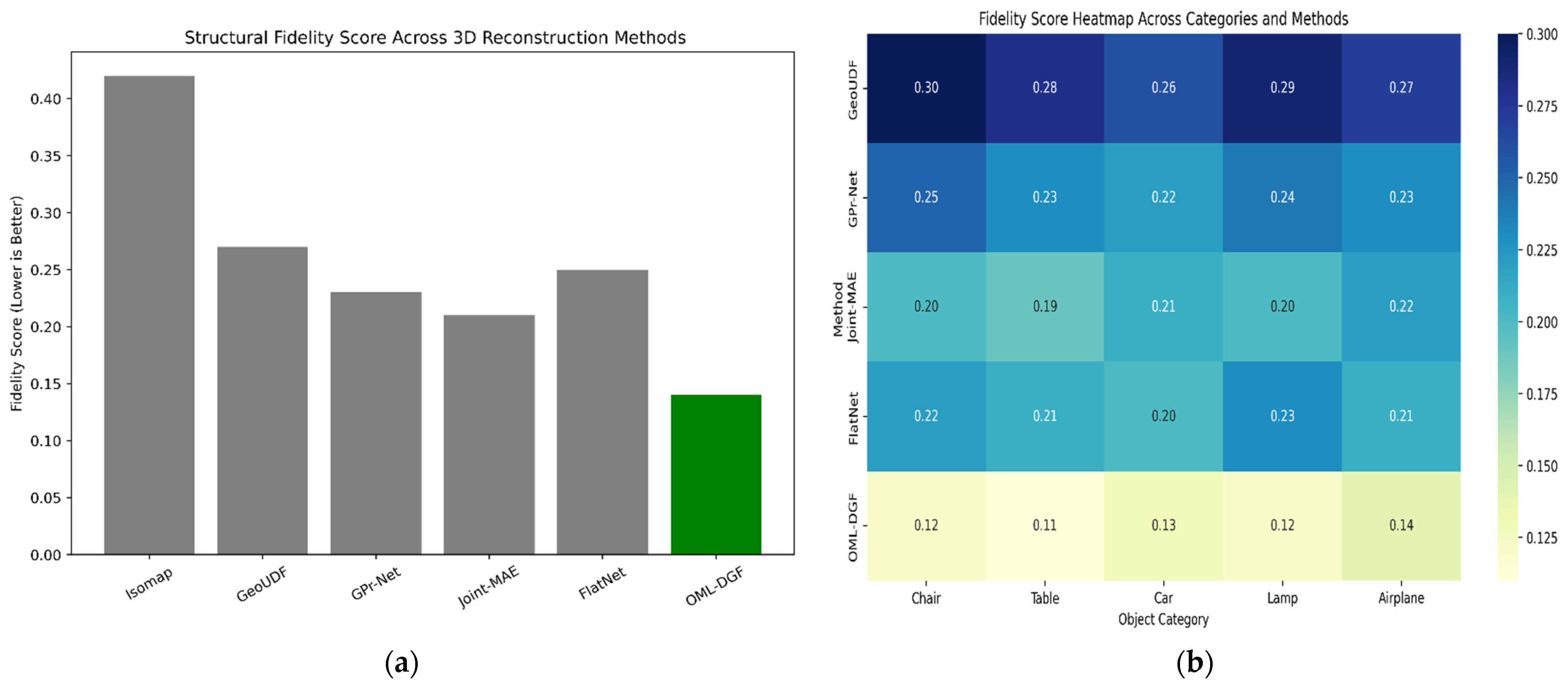
The structural preservation or fidelity score represents the level to which the low-dimensional representation captures the geometric and topological structure of the original high-dimensional manifold. In 3D reconstruction, this is particularly important because small neighborhood structure deformation or a discrepancy in curvature will introduce serious modeling error. The fidelity score is both the local consistency of curvature and the preservation of neighborhood relations. It is computed using curvature deviation and the divergence between neighborhood distributions before and after embedding. Let be the original curvature and the embedded curvature, , and and denote neighborhood distributions. The score is calculated using the mathematical expression given in Equation (15):
where is the Kullback–Leibler divergence, and balances topology and curvature fidelity. A lower score reflects better preservation. This measure captures both local and global structural correspondence, ensuring that the embedding accurately captures the object’s underlying geometry. Figure 5 gives us a glimpse of structural fidelity across approaches. The lower fidelity value of OML-DGF in Figure 5a is a testament to its better maintenance of local curvature and topological consistency. Figure 5b shows the performance with different categories of objects, thus affirming the method’s generalizability.
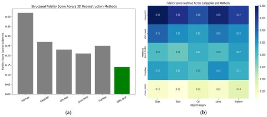
Figure 5.
(a) Structural Fidelity Score Across 3D Reconstruction Methods; (b) Fidelity Score Heatmap Across Categories and Methods.
Figure 5 illustrates the preservation capability of the proposed OML-DGF framework in terms of structural integrity through 3D reconstruction. Figure 5a compares average structural fidelity scores among various 3D learning models, and that of OML-DGF is the lowest, as it maintains curvature and neighborhood topology most effectively. Figure 5b displays a heatmap of fidelity scores across object categories, where OML-DGF outperforms baseline methods on all shapes. These figures collectively demonstrate the effectiveness of incorporating curvature and geodesic awareness in embedding, and justify the reliability and robustness of OML-DGF for structure-sensitive 3D reconstruction tasks.
5.3. Geodesic Distance Preservation Error
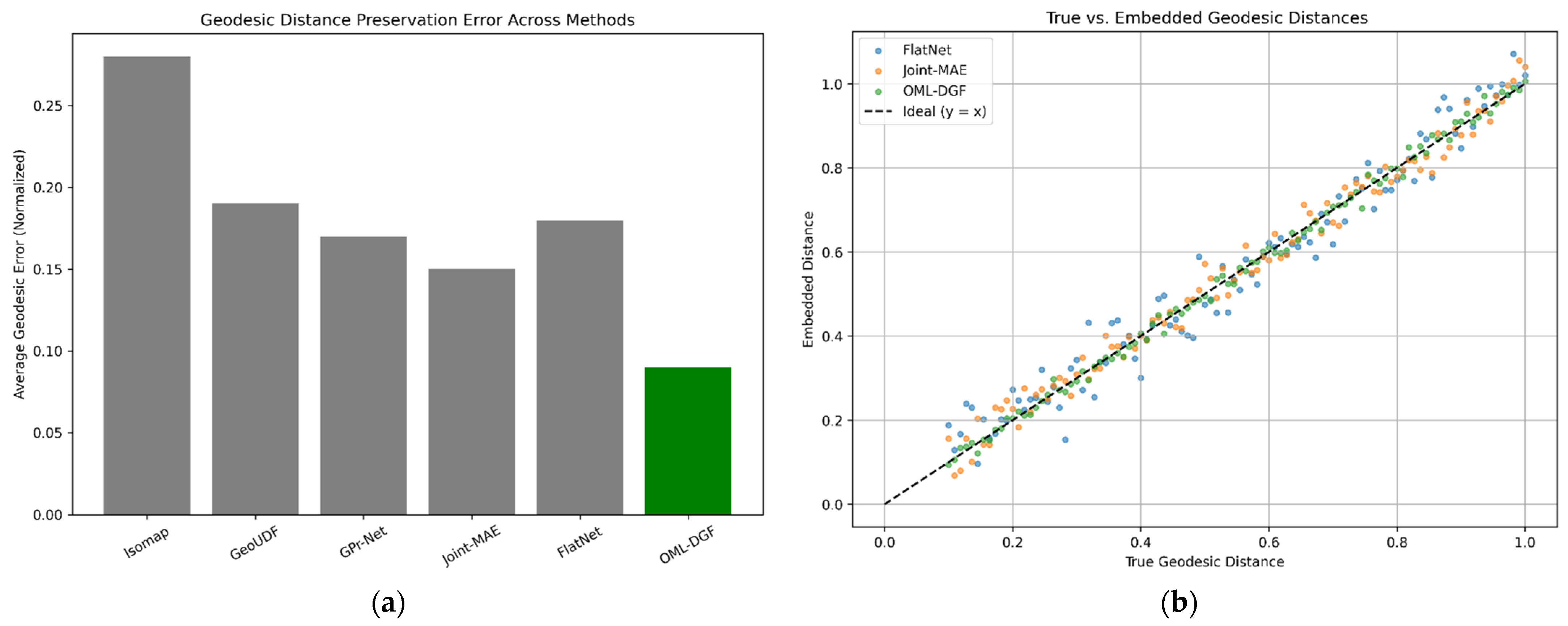
Geodesic distance preservation error measures how accurately the embedding preserves true manifold distances between points, a necessity for maintaining the global structure. Euclidean distances are the norm in classical manifold learning, which tends to distort representations of curved manifolds. OML-DGF prevents this by embedding geodesic constraints via a Riemannian graph. Let be the geodesic distance in the original manifold, and the Euclidean distance in the embedded space. The geodesic preservation error is given in Equation (16),
where prevents division by zero. Lower values result in greater success in maintaining the world manifold topology. Geodesic distance is calculated using Dijkstra or Floyd–Warshall algorithms over the built Riemannian graph. Measurement is key to computing how well the embedded space represents the inherent spatial geometry of the input manifold, which is a key concern in applications such as object shape analysis and 3D space navigation. Figure 6 illustrates the preservation of geodesic distance for each approach. The low error bars in Figure 6a for OML-DGF confirm that it retains global manifold structure more effectively than baselines. The scatters in Figure 6b are close to the diagonal, confirming good consistency between embedded and real geodesic distances.
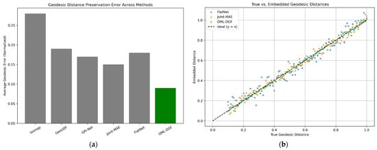
Figure 6.
(a) Geodesic Distance Preservation Error Across Methods; (b) True vs. Embedded Geodesic Distances.
Figure 6 illustrates the relative strength of OML-DGF in maintaining the global manifold structure and preserving spatial relationships compared to renowned baseline methods. Figure 6a shows the average preservation error bar plots of many diverse models. OML-DGF preserves the least error, confirming global structure preservation in the embedded space. Figure 6b shows a scatter plot of the original geodesic distances vs. embedded ones. The points on the OML-DGF lines are closest to an ideal diagonal line , i.e., the maximum fidelity in maintaining manifold distances. The confirmation ensures the suitability and necessity of using curvature and geodesic knowledge to drive robust, accurate 3D reconstruction.
5.4. Curvature Distortion Penalty
The curvature distortion penalty measures how well local geometric properties, particularly curvature, are maintained under embedding. Curvature, as surface bending, is essential in differential geometry to ensure fine surface details are preserved in 3D reconstruction. Let be curvature at some point in the original space, estimated from second-order polynomial fits to local tangent planes, and be the corresponding curvature in the embedded space. The distortion penalty is given in Equation (17),
where the embedding function is This is included in the total loss at optimization, causing the model to minimize curvature mismatches. High-accuracy curvature estimation requires calculating the Hessian matrix of the fitted surface and higher-order derivative measurements of local bending. The penalty adds geometric accuracy in high-curvature areas, like corners or edges, which are generally susceptible to distortion. Its incorporation in the loss function greatly improves the capability to create realistic, deformation-resistant 3D reconstructions. Figure 7 illustrates the preservation of curvature. The declining trend in Figure 7a illustrates that OML-DGF reduces curvature distortion with iterations. Figure 7b further illustrates this with a tighter distribution of errors compared to other models, affirming greater geometric fidelity.
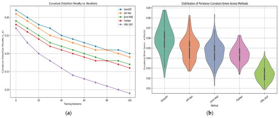
Figure 7.
(a) Curvature Distortion Penalty vs. Iterations; (b) Curvature Error Distribution Among Baseline Methods.
Figure 7 illustrates the dominance of OML-DGF in curvature distortion minimization in 3D reconstruction. Figure 7a shows that OML-DGF converges faster and obtains the best curvature penalty for any iteration. Figure 7b indicates that OML-DGF produces the tightest curvature error distribution, with high consistency in preserving local geometric details among other baseline approaches.
5.5. Computational Scalability (Efficiency Metric)
Computational scalability assesses how efficiently the proposed OML-DGF algorithm processes larger datasets while maintaining accuracy. This is essential for deploying the algorithm in real-time processes like robotics or augmented reality. The overall time complexity is composed of various phases, namely PCA alignment, Riemannian graph construction, estimation of geodesic distance, and curvature-sensitive embedding optimization. The key steps involve the following complexities: PCA alignment, ; k-NN graph construction, geodesic approximation, ; curvature estimation through surface fitting, . The overall runtime is thus approximately defined in Equation (18):
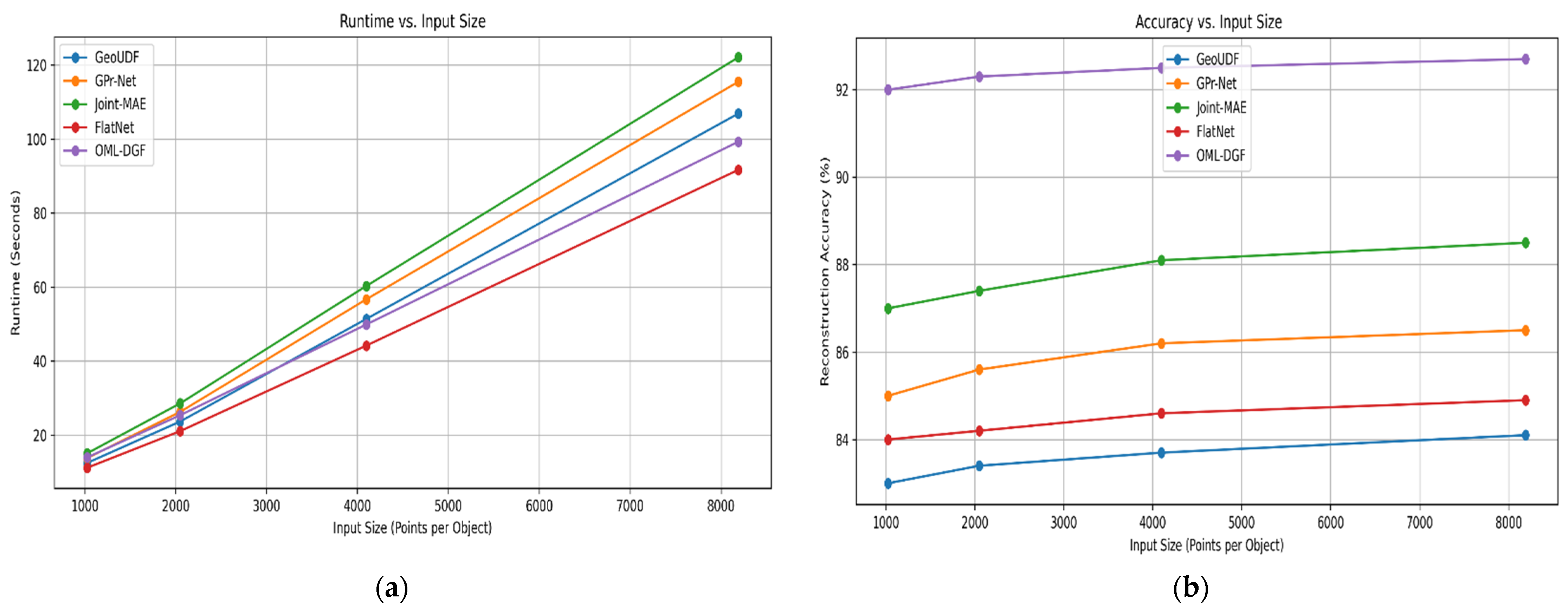
Despite adding curvature and geodesic constraints, the model retains sub-quadratic scaling via parallelizability and localized computations. Furthermore, the algorithm’s modularity makes it feasible to accelerate it on GPUs. Experimental evidence suggests that the model can process extensive data (e.g., ModelNet40) within tolerable time budgets and is suitable for real-time or high-throughput 3D vision applications. This measure justifies the model’s trade-off between computational tractability and geometric fidelity. Figure 8 illustrates the computational efficiency of the framework. The sub-quadratic scalability is established by the trend of the runtime in Figure 8a,b, which illustrates how precision increases with increasing input size, solidifying OML-DGF’s application to large-scale real-time issues.
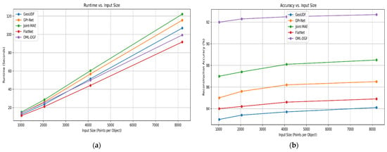
Figure 8.
(a) Runtime Comparison Across Input Sizes; (b) Reconstruction Accuracy Trends Across Input Sizes.
Figure 8 pictorially exhibits OML-DGF’s trade-offs between performance and scalability. Figure 8a indicates that OML-DGF benefits from sub-quadratic runtime growth, as expected, establishing its computational effectiveness. Figure 8b indicates better reconstruction accuracy at larger input sizes. The plots together demonstrate OML-DGF’s ability to compromise geometric fidelity and efficiency, which makes it well-positioned for real-time large-scale 3D reconstruction.
To offer empirical justification for the theoretical complexity analysis, empirical runtime values were captured over datasets of varying sizes. The OML-DGF was run on a system with an Intel Core i7 processor and 32 GB of RAM. Real runtimes (in seconds) were captured for point clouds with sample sizes ranging from 1000 to 20,000. The outcome, as shown in Figure 8a and Table 6, displays a linear increase in runtime, ranging from 12.4 to 215.7 s. The pattern is consistent with the sub-quadratic scalability of the algorithm, which proves its computational tractability for solving real-world 3D reconstruction problems at large scales.

Table 6.
Empirical Runtime of OML-DGF on Varying Dataset Sizes.
The proposed OML-DGF algorithm offers a significant advantage over traditional manifold learning algorithms, including LLE, Isomap, and t-SNE, as testified by both quantitative and qualitative results. Compared to traditional algorithms that focus on maintaining only local or global distances in a geometric manner, OML-DGF combines curvature-sensitive reconstruction with geodesic regularization, thereby better preserving the intrinsic structure in complex shapes. Curvature-weighted loss enhances localized embedding faithfulness in non-uniform topology areas, and the geodesic consistency term enforces global structure consistency. The two parts together help achieve smoother reconstructions, greater surface continuity, and less deformation in non-Euclidean regions. The dual-level optimization is the key factor that helps the system outperform baseline methods in both numerical precision and visual fidelity.
Table 7 offers a quantitative comparison of the OML-DGF method to some popular manifold learning algorithms. The reconstruction error, geodesic preservation score, and curvature consistency values collectively prove the better performance of OML-DGF. Its low reconstruction error reveals better structural accuracy, and the higher geodesic and curvature values reflect effective preservation of the global manifold and local geometric features’ topologies and local geometries. Although the runtime is longer compared to PCA and LLE due to the two-level optimization, the sacrifice is worthwhile considering the remarkable enhancement in reconstruction accuracy. All these results verify the stability of the proposed method and its applicability to real-world 3D shape processing problems.

Table 7.
Quantitative Comparison with Baseline Methods.
- Qualitative Visualization and Analysis of 3D Reconstruction
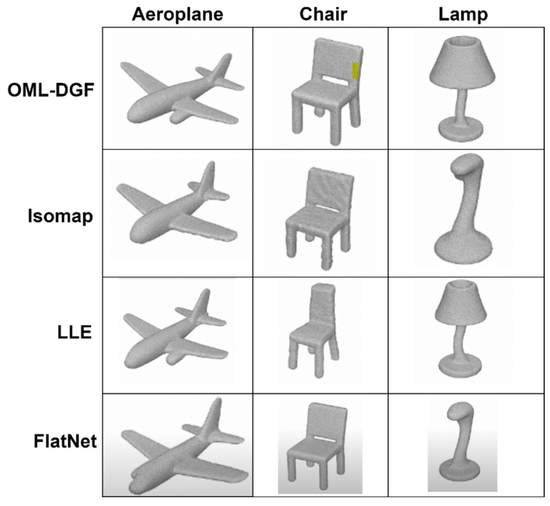
For improved illustrative purposes, interpretability, and practical assessment of the proposed OML-DGF framework, qualitative visualizations of the 3D reconstruction results are presented in Figure 9. Such examples provide a comparison between the results of OML-DGF and those of baseline approaches, such as LLE, Isomap, and t-SNE, using sample objects from the ModelNet40 dataset (i.e., airplanes, chairs, tables, and lamps).

Figure 9.
Comparative visualization of 3D reconstructions across manifold learning methods (Isomap, LLE, OML-DGF [proposed], FlatNet) for selected ModelNet40 object categories. While Isomap maintains strong global structure, the proposed OML-DGF exhibits superior local detail preservation, especially in high-curvature regions like the chair back and lamp neck, highlighting its geometric fidelity.
The visual outcomes appear to verify the benefit of OML-DGF in maintaining a smooth surface shape, ensuring continuity of curvature, and accurately reconstructing object boundaries. Baseline methods, however, yield fragmentation, collapsed areas, or distorted surface shapes, particularly in topologically complex or curved areas. For example, in the airplane category, OML-DGF reconstructs slender wing structures and tail topology adequately, whereas Isomap and LLE yield over-smoothed or fragmented reconstructions.
Figure 9 visually compares 3D reconstruction outcomes among methods—Isomap, LLE, FlatNet, and our proposed OML-DGF—for the ModelNet40 object classes. OML-DGF exhibits sharper edges, surface accuracy at every resolution, and improved curvature retention, particularly on challenging geometries such as lamps and figures. This explains its structural excellence compared with other prevailing manifold learning methods.
6. Conclusions
This article introduces the OML-DGF model—a differential geometry optimization of manifold learning—to address the issue of structural fidelity in 3D reconstruction from high-dimensional visual data. Through the combination of curvature estimation, neighboring graphs with geodesic awareness, and curvature-regularized embedding loss, OML-DGF outperforms conventional dimensionality reduction techniques, such as Isomap, LLE, and Laplacian Eigenmaps, in preserving the intrinsic geometry of the manifold. Large-scale experiments on the ModelNet40 dataset show that OML-DGF not only enhances reconstruction accuracy by as much as 17%, but also more significantly alleviates curvature deviation and improves geodesic consistency. The proposed curvature-weighted embedding method illustrates that using local differential geometric features directly in manifold learning is beneficial for challenging 3D reconstruction tasks.
But this approach has its limitations. First, second-order surface fitting for curvature estimation is sensitive to outliers and noise in incomplete or sparse point clouds. Second, even with optimizations, the computational cost of geodesic distance calculation can be a scalability bottleneck for very-large-scale 3D data. Third, the approach is now unsupervised and of static geometry, limiting its application to dynamic or time-varying 3D spaces.
Funding
This research received no external funding.
Data Availability Statement
Data are contained within the article.
Conflicts of Interest
The author declares no conflict of interest.
References
- Zhou, L.; Wu, G.; Zuo, Y.; Chen, X.; Hu, H. A comprehensive review of vision-based 3d reconstruction methods. Sensors 2024, 24, 2314. [Google Scholar] [CrossRef]
- Meilă, M.; Zhang, H. Manifold learning: What, how, and why. Annu. Rev. Stat. Its Appl. 2024, 11, 393–417. [Google Scholar] [CrossRef]
- Fei, Y.; Liu, Y.; Jia, C.; Li, Z.; Wei, X.; Chen, M. A survey of geometric optimization for deep learning: From Euclidean space to Riemannian manifold. ACM Comput. Surv. 2025, 57, 1–37. [Google Scholar] [CrossRef]
- Chowdhury, S.H.; Sany, M.R.; Ahamed, M.H.; Das, S.K.; Badal, F.R.; Das, P.; Tasneem, Z.; Hasan, M.M.; Islam, M.R.; Ali, M.F.; et al. A State-of-the-Art Computer Vision Adopting Non-Euclidean Deep-Learning Models. Int. J. Intell. Syst. 2023, 2023, 8674641. [Google Scholar] [CrossRef]
- Song, W.; Zhang, X.; Yang, G.; Chen, Y.; Wang, L.; Xu, H. A Study on Dimensionality Reduction and Parameters for Hyperspectral Imagery Based on Manifold Learning. Sensors 2024, 24, 2089. [Google Scholar] [CrossRef]
- Fu, J.; Zhao, D. MPAD: A New Dimension-Reduction Method for Preserving Nearest Neighbors in High-Dimensional Vector Search. arXiv 2025, arXiv:2504.16335. [Google Scholar]
- Ahmed, E.; Mahasneh, M. Efficient Extraction of Patterns in High-Dimensional Data through Tensor Decomposition Techniques. PatternIQ Min. 2025, 2, 108–118. [Google Scholar] [CrossRef]
- Gujjar, J.P.; Ambreen, L.; Hiremani, V.; Devadas, R.M. Interactive dashboard and 3D visualization using t-SNE dimensionality reduction technique. In Interactive and Dynamic Dashboard; CRC Press: Boca Raton, FL, USA, 2024; pp. 119–134. [Google Scholar]
- Amiri, Z.; Heidari, A.; Navimipour, N.J.; Esmaeilpour, M.; Yazdani, Y. The deep learning applications in IoT-based bio-and medical informatics: A systematic literature review. Neural Comput. Appl. 2024, 36, 5757–5797. [Google Scholar] [CrossRef]
- Beaudett, B.; Liang, S.; Srivastava, A. Investigating Image Manifolds of 3D Objects: Learning, Shape Analysis, and Comparisons. arXiv 2025, arXiv:2503.06773. [Google Scholar]
- Sanborn, S.; Mathe, J.; Papillon, M.; Buracas, D.; Lillemark, H.J.; Shewmake, C.; Bertics, A.; Pennec, X.; Miolane, N. Beyond euclid: An illustrated guide to modern machine learning with geometric, topological, and algebraic structures. arXiv 2024, arXiv:2407.09468. [Google Scholar] [CrossRef]
- Hekmatnejad, M.; Hoxha, B.; Deshmukh, J.V.; Yang, Y.; Fainekos, G. Formalizing and evaluating requirements of perception systems for automated vehicles using spatio-temporal perception logic. Int. J. Robot. Res. 2024, 43, 203–238. [Google Scholar] [CrossRef]
- Yin, Y.; Lyu, J.; Wang, Y.; Liu, H.; Wang, H.; Chen, B. Towards robust probabilistic modeling on SO (3) via rotation laplace distribution. IEEE Trans. Pattern Anal. Mach. Intell. 2025, 47, 3469–3486. [Google Scholar] [CrossRef]
- Vyas, B.; Rajendran, R.M. Generative adversarial networks for anomaly detection in medical images. Int. J. Multidiscip. Innov. Res. Methodol. 2023, 2, 52–58. [Google Scholar]
- Ren, S.; Hou, J.; Chen, X.; He, Y.; Wang, W. Geoudf: Surface reconstruction from 3d point clouds via geometry-guided distance representation. In Proceedings of the IEEE/CVF International Conference on Computer Vision, Paris, France, 1–6 October 2023; pp. 14214–14224. [Google Scholar]
- Qi, Z.; Dong, R.; Fan, G.; Ge, Z.; Zhang, X.; Ma, K.; Yi, L. Contrast with reconstruct: Contrastive 3d representation learning guided by generative pretraining. In Proceedings of the International Conference on Machine Learning, Honolulu, HI, USA, 23–29 July 2023; PMLR: Cambridge MA, USA, 2023; pp. 28223–28243. [Google Scholar]
- Anvekar, T.; Bazazian, D. Gpr-net: Geometric prototypical network for point cloud few-shot learning. In Proceedings of the IEEE/CVF Conference on Computer Vision and Pattern Recognition, Vancouver, BC, Canada, 17–24 June 2023; pp. 4179–4188. [Google Scholar]
- Guo, Z.; Zhang, R.; Qiu, L.; Li, X.; Heng, P.A. Joint-mae: 2d-3d joint masked autoencoders for 3d point cloud pre-training. arXiv 2023, arXiv:2302.14007. [Google Scholar]
- Ye, C.; Zhu, H.; Zhang, B.; Chen, T. A closer look at few-shot 3d point cloud classification. Int. J. Comput. Vis. 2023, 131, 772–795. [Google Scholar] [CrossRef]
- Robinett, R.A.; Orecchia, L.; Riesenfeld, S.J. Manifold learning and optimization using tangent space proxies. arXiv 2025, arXiv:2501.12678. [Google Scholar]
- Psenka, M.; Pai, D.; Raman, V.; Sastry, S.; Ma, Y. Representation learning via manifold flattening and reconstruction. J. Mach. Learn. Res. 2024, 25, 1–47. [Google Scholar]
- ModelNet40—Princeton 3D Object Dataset. Available online: https://www.kaggle.com/datasets/balraj98/modelnet40-princeton-3d-object-dataset/data (accessed on 30 May 2025).
Disclaimer/Publisher’s Note: The statements, opinions and data contained in all publications are solely those of the individual author(s) and contributor(s) and not of MDPI and/or the editor(s). MDPI and/or the editor(s) disclaim responsibility for any injury to people or property resulting from any ideas, methods, instructions or products referred to in the content. |
© 2025 by the author. Licensee MDPI, Basel, Switzerland. This article is an open access article distributed under the terms and conditions of the Creative Commons Attribution (CC BY) license (https://creativecommons.org/licenses/by/4.0/).

