Inhomogeneous Whittaker Equation with Initial and Boundary Conditions

Abstract

In this study, a semi-analytical solution to the inhomogeneous Whittaker equation is developed for both initial and boundary value problems. A new class of special integral functions ${}^f\mathrm{Zi}_{\kappa ,\mu }\left(x\right)$, along with their derivatives, is introduced to facilitate the construction of the solution. The analytical properties of ${}^f\mathrm{Zi}_{\kappa ,\mu }\left(x\right)$ are rigorously investigated, and explicit closed-form expressions for ${}^f\mathrm{Zi}_{\kappa ,\mu }\left(x\right)$ and its derivatives are derived in terms of Whittaker functions ${\mathrm{M}}_{\kappa ,\mu }\left(z\right)$ and ${\mathrm{W}}_{\kappa ,\mu }\left(z\right)$, confluent hypergeometric functions, and other special functions including Bessel functions, modified Bessel functions, and the incomplete gamma functions, along with their respective derivatives. These expressions are obtained for specific parameter values using symbolic computation in Maple. The results contribute to the broader analytical framework for solving inhomogeneous linear differential equations with applications in engineering, mathematical physics, and biological modeling.

1. Introduction

The homogeneous Whittaker equation, first formulated in 1903, represents a classical second-order linear differential equation and is expressed in the form [1]:

$${\displaystyle \frac{{\mathrm{d}}^2\mathrm{W}}{\mathrm{d}{z}^2}}+\left(-{\displaystyle \frac{1}{4}}+{\displaystyle \frac{\kappa }{z}}+{\displaystyle \frac{\frac{1}{4}-{\mu }^2}{z^2}}\right)\mathrm{W}=0,$$

(1)

wherein $\kappa$ and $\mu$ are parameters and z and $\mathrm{W}$ are variables that could be real or complex. Whittaker [1] introduced the functions ${\mathrm{M}}_{\kappa ,\mu }\left(z\right)$ and ${\mathrm{W}}_{\kappa ,\mu }\left(z\right)$ as linearly independent solutions to the homogeneous Whittaker equation. The pairs of functions ${\mathrm{M}}_{\kappa ,\mu }\left(z\right)$, ${\mathrm{M}}_{\kappa ,-\mu }\left(z\right)$ and ${\mathrm{W}}_{\kappa ,\mu }\left(z\right),{\mathrm{W}}_{-\kappa ,\mu }\left(z\right)$ discussed below are linearly independent solutions of Equation (1). The Wronskian of the Whittaker functions is provided in detail in [2]:

$$\begin{array}{c}\mathcal{W}\left\{{\mathrm{M}}_{\kappa ,\mu }\left(z\right),{\mathrm{M}}_{\kappa ,-\mu }\left(z\right)\right\}=-2\mu ,\\ \mathcal{W}\left\{{\mathrm{M}}_{\kappa ,\mu }\left(z\right),{\mathrm{W}}_{\kappa ,\mu }\left(z\right)\right\}=-{\displaystyle \frac{\Gamma (1+2\mu )}{\Gamma \left(\frac{1}{2}+\mu -\kappa \right)}},\\ \mathcal{W}\left\{{\mathrm{M}}_{\kappa ,\mu }\left(z\right),{\mathrm{W}}_{-\kappa ,\mu }\left({\mathrm{e}}^{\pm \pi \mathrm{i}}z\right)\right\}={\displaystyle \frac{\Gamma (1+2\mu )}{\Gamma \left(\frac{1}{2}+\mu +\kappa \right)}}{\mathrm{e}}^{\mp \left({\displaystyle \frac{1}{2}}+\mu \right)\pi \mathrm{i}},\\ \mathcal{W}\left\{{\mathrm{M}}_{\kappa ,-\mu }\left(z\right),{\mathrm{W}}_{\kappa ,\mu }\left(z\right)\right\}=-{\displaystyle \frac{\Gamma (1-2\mu )}{\Gamma \left(\frac{1}{2}-\mu -\kappa \right)}}.\end{array}$$

(2)

Equation (1) represents the reduced form of a degenerate hypergeometric equation and possesses a regular singular point at $z=0$ and an irregular singular point at $z=\infty$. A broad class of second-order linear differential equations including Whittaker’s and Weber’s equations can be systematically transformed, through suitable changes of variables and function substitutions, into the canonical confluent hypergeometric form [2]:

$$z{\displaystyle \frac{{\mathrm{d}}^{2}w}{\mathrm{d}{z}^2}}+(b-z){\displaystyle \frac{\mathrm{d}w}{\mathrm{d}z}}-aw=0.$$

(3)

This structural reducibility reveals a profound analytical equivalence among these equations, thereby establishing a unified framework for their investigation. The solution framework for the Whittaker equation, as presented in this work, can be derived from the results in [3] via an appropriate change of variables. This connection not only highlights the versatility of the Whittaker formulation but also underscores the broader applicability of methods developed for the Weber-type equations. In the homogeneous case, the correspondence between their respective solutions and classical special functions is well established in the literature. However, in the inhomogeneous case, the transformation of the forcing term often leads to complicated integrals. These difficulties become particularly pronounced when employing the method of variation of parameters to construct particular solutions, as the transformed forcing function may not yield to standard integration techniques. The solution of the inhomogeneous Weber’s equation has been thoroughly analyzed in [3], where both theoretical and computational aspects are addressed. For practical applications, particularly in fluid dynamics and engineering, refer to [4], which demonstrates the relevance of the inhomogeneous Weber equation in modeling and simulation.

Whittaker’s Equation (1) arises in various areas of physics, particularly in quantum mechanics, and plays a significant role in solving the radial Schrödinger equation in spherical coordinates and in the solution to the wave equation in parabolic coordinates [5], in addition to describing the behavior of charged particles in a Coulomb potential [6]. Akbarzadeh [7] utilized the Whittaker differential equation in deriving an exact, analytical solution for convective heat transfer of thermally fully developed laminar nanofluid flow in a circular tube, where the pipe wall is exposed to a constant temperature. Gupta and Bhengra [8] applied Whittaker functions to the derivation of the dispersion equation governing the propagation of torsional surface waves in an anisotropic layer sandwiched between two anisotropic inhomogeneous media. Conway [9] employed the Wronskian of the Whittaker functions to calculate indefinite integrals involving Whittaker’s functions and their products.

In the analysis of processes governed by time fractional diffusion and diffusion-wave equations, the Whittaker functions are important both as special functions and for their broad applications in mathematical physics, as they play a central role in the theory of uniform asymptotic expansions of differential equations with coalescing turning points and simple poles, as discussed in [2,10,11]. Mainardi et al. [12] compared Wright functions of the second kind with Whittaker functions in specific cases of fractional order. Their work in [12] underscores the importance of Whittaker functions in the context of higher transcendental functions. Szmytkowski and Bielski [13] investigated the orthogonality of Whittaker functions of the second kind, ${\mathrm{W}}_{\kappa ,i\mu }\left(x\right)$, where $\mu \in \mathbb{R}$, with the weight function $w\left(x\right)={\displaystyle \frac{1}{x^2}}$. Chang et al. [14] investigated the asymptotic behavior of the Whittaker function of the second kind for large values of the parameters and the independent variable z. Dunster [15] derived uniform asymptotic expansions for the Whittaker functions $M_{\kappa ,\mu }\left(z\right)$ and $W_{\kappa ,\mu }\left(z\right)$, as well as the numerically satisfactory companion function $W_{-\kappa ,\mu }\left(z{e}^{-\pi i}\right)$. The expansions are uniformly valid for $\mu \to \infty$ and for a specific ratio of the parameters $\kappa$ and $\mu$, with $0\le arg\left(z\right)\le \pi$. Using appropriate connection and analytic continuation, the expansions are extended to all unbounded non-zero complex values of z.

Izarra et al. [16] applied Pade approximants in combination with Wynn’s algorithm on a specific asymptotic expansion to achieve precise numerical computations of the Whittaker functions ${\mathrm{W}}_{\kappa ,\mu }\left(z\right)$ for various values of the argument z and the parameters $\kappa$ and $\mu$. Ragab [17] systematically evaluated integrals involving products of Whittaker and Bessel functions.

A general solution to Equation (1) can be expressed as a linear combination of these two solutions as

$$\begin{array}{cc}\hfill & \mathrm{W}\left(z\right)=C_1{\mathrm{M}}_{\kappa ,\mu }\left(z\right)+C_2{\mathrm{W}}_{\kappa ,\mu }\left(z\right),\hfill \\ \hfill & 2\mu \ne -1,-2,\dots ,\hfill \end{array}$$

(4)

where $\kappa$ and $\mu$ are parameters.

The Whittaker functions can be expressed as [2]:

$$\begin{array}{cc}\hfill & {\mathrm{M}}_{\kappa ,\mu }\left(z\right)={\mathrm{e}}^{-{\displaystyle \frac{1}{2}}z}{z}^{{\displaystyle \frac{1}{2}}+\mu }M\left({\displaystyle \frac{1}{2}}+\mu -\kappa ,1+2\mu ,z\right),\hfill \\ \hfill & {\mathrm{W}}_{\kappa ,\mu }\left(z\right)={\mathrm{e}}^{-{\displaystyle \frac{1}{2}}z}{z}^{{\displaystyle \frac{1}{2}}+\mu }\mathrm{U}\left({\displaystyle \frac{1}{2}}+\mu -\kappa ,1+2\mu ,z\right),\hfill \end{array}$$

(5)

where $M(a,b,z):={}_{1}F_1(a;b;z)$ denotes Kummer’s confluent hypergeometric function of the first kind, and $\mathrm{U}(a,b;z)$ denotes the confluent hypergeometric function of the second kind (also known as Tricomi’s function). The functions $M(a,b,z)$ and $\mathrm{U}(a,b,z)$ constitute the two standard linearly independent solutions of the confluent hypergeometric differential Equation (3). Their definitions are given as follows [2]:

$$M(a,b,z)=\sum _{s=0}^{\infty }{\displaystyle \frac{{\left(a\right)}_s}{{\left(b\right)}_{s}s!}}{z}^s=1+{\displaystyle \frac{a}{b}}z+{\displaystyle \frac{a(a+1)}{b(b+1)2!}}{z}^2+\dots ,$$

(6)

where ${\left(a\right)}_s$ denotes the Pochhammer symbol, defined by ${\left(a\right)}_s=a(a+1)\dots (a+s-1)$ for $s\ge 1$, with ${\left(a\right)}_0=1$. For non-integer values of b, the function $\mathrm{U}(a,b;z)$ can be expressed in terms of $M(a,b,z)$:

$$\mathrm{U}(a,b;z)={\displaystyle \frac{\Gamma (1-b)}{\Gamma (a-b+1)}}M(a,b,z)+{\displaystyle \frac{\Gamma (b-1)}{\Gamma \left(a\right)}}{z}^{1-b}M(a-b+1,2-b,z).$$

(7)

Equation (7) is equivalent to [18]:

$$\mathrm{U}(a,b,z)={\displaystyle \frac{\pi }{sin\left(\pi b\right)}}\left[{\displaystyle \frac{M(a,b,z)}{\Gamma (1+a-b)\Gamma \left(b\right)}}-z^{1-b}{\displaystyle \frac{M(1+a-b,2-b,z)}{\Gamma \left(a\right)\Gamma (2-b)}}\right].$$

(8)

In the case where b assumes integer values, the function $\mathrm{U}(a,b,z)$ can be computed via appropriate limiting procedures or alternative representations, due to singularities at integer values of b, where $sin\left(b\pi \right)=0$, in Equation (8). Regarding the calculation of the function $\mathrm{U}(a,b,z)$ for integer values of the parameter b, the reader is referred to [19]. The function $M_{\kappa ,\mu }\left(z\right)$ is undefined when $2\mu =-1,-2,-3,\dots$. Therefore, hereafter, it is understood that $2\mu =-1,-2,-3,\dots$, unless otherwise specified. For specific values of these parameters, the Whittaker functions ${\mathrm{M}}_{\kappa ,\mu }\left(x\right)$ and ${\mathrm{W}}_{\kappa ,\mu }\left(x\right)$ can be simplified to various elementary and special functions, including modified Bessel functions, incomplete gamma functions, parabolic cylinder functions, error functions, and logarithmic and cosine integrals, as well as generalized Hermite and Laguerre polynomials. For more details, see [20] and the references therein. In view of potential applications to engineering problems, we restrict our analysis of the inhomogeneous Whittaker equation to the case where the independent variable z is real; hence,

$${\mathrm{M}}_{\kappa ,\mu }\left(x\right)=x^{\mu -1/2}{e}^{-x/2}{}_{1}F_1\left(\left.\begin{array}{c}\mu -\kappa +{\displaystyle \frac{1}{2}}\\ 1+2\mu \end{array}\right|x\right).$$

(9)

The Whittaker function ${\mathrm{W}}_{\kappa ,\mu }\left(x\right)$ can be expressed in terms of the Whittaker functions of the first kind ${\mathrm{M}}_{\kappa ,\mu }\left(x\right)$, provided that $2\mu \notin \mathbb{Z}$, as follows [10,11]:

$${\mathrm{W}}_{\kappa ,\mu }\left(x\right)={\displaystyle \frac{\Gamma (-2\mu )}{\Gamma \left(\frac{1}{2}-k-\mu \right)}}{\mathrm{M}}_{\kappa ,\mu }\left(x\right)+{\displaystyle \frac{\Gamma \left(2\mu \right)}{\Gamma \left(\frac{1}{2}-k+\mu \right)}}{\mathrm{M}}_{\kappa ,-\mu }\left(x\right).$$

(10)

It is important to note that both ${\mathrm{M}}_{\kappa ,\mu }\left(x\right)$ and ${\mathrm{M}}_{\kappa ,-\mu }\left(x\right)$ constitute two linearly independent solutions of the homogeneous Whittaker equation.

In this work, we present a method for obtaining the general solution to Whittaker’s inhomogeneous equation. The approach is based on the introduction of an integral function, denoted by ${}^f\mathrm{Zi}_{\kappa ,\mu }\left(x\right)$, whose evaluation relies on a generalization of the Whittaker integrals previously discussed by Appleblatt and Santandar [20]. Accordingly, the function ${}^f\mathrm{Zi}_{\kappa ,\mu }\left(x\right)$ serves as a fundamental instrument for representing solutions to the initial and boundary value problems associated with the inhomogeneous Whittaker equation.

To achieve this objective, the manuscript is organized as follows.

Section 2 introduces the inhomogeneous Whittaker equation and presents the function ${}^f\mathrm{Zi}_{\kappa ,\mu }\left(x\right)$ as part of its solution. The section also outlines the properties of ${}^f\mathrm{Zi}_{\kappa ,\mu }\left(x\right)$ and explains how it can be evaluated. In Section 3, we evaluate the function ${}^f\mathrm{Zi}_{\kappa ,\mu }\left(x\right)$ for specific parameter values and various forms of the function $f\left(x\right)$. Section 4 presents the derivative of ${}^f\mathrm{Zi}_{\kappa ,\mu }\left(x\right)$, derived using the known derivatives of the Whittaker functions. In Section 5, we provide solutions to the inhomogeneous Whittaker differential equation for both initial and boundary value problems. Finally, the conclusion summarizes the key results and suggests possible directions for future research.

2. Inhomogeneous Whittaker Equation

In this section, we will investigate the inhomogeneous Whittaker equation, which is given by

$${\displaystyle \frac{{\mathrm{d}}^{2}W}{\mathrm{d}{x}^2}}+\left(-{\displaystyle \frac{1}{4}}+{\displaystyle \frac{\kappa }{x}}+{\displaystyle \frac{\frac{1}{4}-{\mu }^2}{x^2}}\right)W=f\left(x\right).$$

(11)

A particular solution to the differential equation can be found using the method of variation of parameters. To this end, we introduce the following function:

$${}^f\mathrm{Zi}_{\kappa ,\mu }\left(x\right)=\left[{\mathrm{M}}_{\kappa ,\mu }\left(x\right){\int }_0^{x}f\left(t\right){\mathrm{W}}_{\kappa ,\mu }\left(t\right)dt-{\mathrm{W}}_{\kappa ,\mu }\left(x\right){\int }_0^{x}f\left(t\right){\mathrm{M}}_{\kappa ,\mu }\left(t\right)dt\right].$$

(12)

The principal role of the integral function ${}^f\mathrm{Zi}_{\kappa ,\mu }\left(x\right)$ is to underpin the formulation of solutions to the inhomogeneous Whittaker equation. Accordingly, we commence the analysis with the following foundational theorem.

Theorem 1.

The general solution of the inhomogeneous Whittaker Equation (11) is given by

$$\begin{array}{cc}\hfill & \mathrm{W}\left(x\right)=C_1{\mathrm{M}}_{\kappa ,\mu }\left(x\right)+C_2{\mathrm{W}}_{\kappa ,\mu }\left(x\right)+{\displaystyle \frac{\Gamma \left(\frac{1}{2}+\mu -\kappa \right)}{\Gamma (1+2\mu )}}{}^f\mathrm{Zi}_{\kappa ,\mu }\left(x\right),\hfill \\ \hfill & 2\mu \ne -1,-2,\dots \hfill \end{array}$$

(13)

Proof. 

The general solution of (11) can be expressed as

$$W\left(x\right)=W_h\left(x\right)+W_p\left(x\right),$$

(14)

where $W_h\left(x\right)$ denotes the general solution of the associated homogeneous equation, whereas $W_p\left(x\right)$ corresponds to a particular solution of the inhomogeneous problem. The homogeneous solution $W_h\left(x\right)$ is given by Equation (4); hence,

$$W_h\left(x\right)=C_1{\mathrm{M}}_{\kappa ,\mu }\left(x\right)+C_2{\mathrm{W}}_{\kappa ,\mu }\left(x\right).$$

(15)

To complete the solution, it remains to construct a particular solution. This is achieved through the method of variation of parameters, yielding the following expression:

$$W_p\left(x\right)=-{\mathrm{M}}_{\kappa ,\mu }\left(x\right){\int }_0^x{\displaystyle \frac{{\mathrm{W}}_{\kappa ,\mu }\left(t\right)f\left(t\right)}{\mathcal{W}\left\{M_{\kappa ,\mu }\left(t\right),W_{\kappa ,\mu }\left(t\right)\right\}}}dt+{\mathrm{W}}_{\kappa ,\mu }\left(x\right){\int }_0^x{\displaystyle \frac{{\mathrm{M}}_{\kappa ,\mu }\left(t\right)f\left(t\right)}{\mathcal{W}\left\{M_{\kappa ,\mu }\left(t\right),W_{\kappa ,\mu }\left(t\right)\right\}}}dt.$$

(16)

The Wronskian $\mathcal{W}\left\{M_{\kappa ,\mu }\left(x\right),W_{\kappa ,\mu }\left(x\right)\right\}$ of the Whittaker functions is given in Equation (2) as

$$\mathcal{W}\left\{M_{\kappa ,\mu }\left(x\right),W_{\kappa ,\mu }\left(x\right)\right\}=-{\displaystyle \frac{\Gamma (1+2\mu )}{\Gamma \left(\frac{1}{2}+\mu -\kappa \right)}}.$$

(17)

By substituting Equation (17) into Equation (16) and simplifying, we obtain a particular solution to Equation (11) given by

$$\begin{array}{cc}\hfill & W_p\left(x\right)={\displaystyle \frac{\Gamma \left(\frac{1}{2}+\mu -\kappa \right)}{\Gamma (1+2\mu )}}{}^f\mathrm{Zi}_{\kappa ,\mu }\left(x\right)\hfill \\ \hfill & 2\mu \ne -1,-2,\dots \hfill \end{array}$$

(18)

Using Equations (4) and (18), a general solution of the inhomogeneous Whittaker Equation (11) is given by

$$\begin{array}{cc}\hfill & W\left(x\right)=C_1{\mathrm{M}}_{\kappa ,\mu }\left(x\right)+C_2{\mathrm{W}}_{\kappa ,\mu }\left(x\right)+{\displaystyle \frac{\Gamma \left(\frac{1}{2}+\mu -\kappa \right)}{\Gamma (1+2\mu )}}{}^f\mathrm{Zi}_{\kappa ,\mu }\left(x\right),\hfill \\ \hfill & 2\mu \ne -1,-2,\dots \hfill \end{array}$$

(19)

□

The properties of the function ${}^f\mathrm{Zi}_{\kappa ,\mu }\left(x\right)$ are influenced by the properties of the Whittaker functions for different values of the parameters $\kappa$ and $\mu$, as well as by the characteristics of the function $f\left(x\right)$. Before presenting a solution to the inhomogeneous Whittaker equation, we will first investigate the function ${}^f\mathrm{Zi}_{\kappa ,\mu }\left(x\right)$ for various parameter values and different forms of $f\left(x\right)$.

In their analysis of integrals involving Whittaker functions, Apelblat et al. [20] define the integral functions ${\mathrm{Mi}}_{\kappa ,\mu }\left(x\right)$ and ${\mathrm{Wi}}_{\kappa ,\mu }\left(x\right)$ that can offer examples of the function ${}^f\mathrm{Zi}_{\kappa ,\mu }\left(x\right)$ for various parameter values, especially when $f\left(x\right)={\displaystyle \frac{1}{x}}$. These Whittaker integral functions are defined as follows [20]:

$${\mathrm{Mi}}_{\kappa ,\mu }\left(x\right)={\int }_0^x{\displaystyle \frac{{\mathrm{M}}_{\kappa ,\mu }\left(t\right)}{t}}dt$$

(20)

and

$${\mathrm{Wi}}_{\kappa ,\mu }\left(x\right)={\int }_0^x{\displaystyle \frac{{\mathrm{W}}_{\kappa ,\mu }\left(t\right)}{t}}dt.$$

(21)

For simplicity, we will generalize the notation from [20] as follows:

$$\begin{array}{c}{}^f\mathrm{Mi}_{\kappa ,\mu }\left(x\right)={\int }_0^{x}f\left(t\right){\mathrm{M}}_{\kappa ,\mu }\left(t\right)dt,\\ {}^f\mathrm{Wi}_{\kappa ,\mu }\left(x\right)={\int }_0^{x}f\left(t\right){\mathrm{W}}_{\kappa ,\mu }\left(t\right)dt.\end{array}$$

(22)

Hence, in the newly introduced generalized notation, the functions

${\mathrm{Mi}}_{\kappa ,\mu }\left(x\right)$ and ${\mathrm{Wi}}_{\kappa ,\mu }\left(x\right)$ are represented as

$$\begin{array}{c}{\mathrm{Mi}}_{\kappa ,\mu }\left(x\right)={}^{\frac{1}{t}}\mathrm{Mi}_{\kappa ,\mu }\left(x\right),\\ {\mathrm{Wi}}_{\kappa ,\mu }\left(x\right)={}^{\frac{1}{t}}\mathrm{Wi}_{\kappa ,\mu }\left(x\right).\end{array}$$

(23)

Therefore, we can rewrite the function ${}^f\mathrm{Zi}_{\kappa ,\mu }\left(z\right)$ given by Equation (12) as follows:

$${}^f\mathrm{Zi}_{\kappa ,\mu }\left(x\right)={\mathrm{M}}_{\kappa ,\mu }\left(x\right){}^f\mathrm{Mi}_{\kappa ,\mu }\left(x\right)-{\mathrm{W}}_{\kappa ,\mu }\left(x\right){}^f\mathrm{Wi}_{\kappa ,\mu }\left(x\right).$$

(24)

From (24), it is easy to see that ${}^f\mathrm{Zi}_{\kappa ,\mu }\left(0\right)=0$. Apelblat et al. [20] used the Mathematica program to express the Whittaker integral functions in terms of elementary special functions and obtained specific cases of the Whittaker integral functions for different values of the parameters $\mu$ and $\kappa$. We used those expressions to derive the following Table 1 for the function ${}^{{\displaystyle \frac{1}{x}}}\mathrm{Zi}_{\kappa ,\mu }\left(x\right)$:

Table 1. Example of ${}^{{\displaystyle \frac{1}{x}}}\mathrm{Zi}_{\kappa ,\mu }\left(z\right)$.

$\mathit{\kappa }$	$\mathit{\mu }$	${}^{\frac{1}{\mathit{x}}}\mathbf{Zi}_{\mathit{\kappa },\mathit{\mu }}\left(\mathit{x}\right)$
${\displaystyle \frac{3}{2}}$	0	$2\sqrt{x}{e}^{-x/2}\left({\mathbf{W}}_{{\displaystyle \frac{3}{2}},0}\left(x\right)-{\mathbf{M}}_{{\displaystyle \frac{3}{2}},0}\left(x\right)\right)$
2	${\displaystyle \frac{1}{2}}$	$x{e}^{-x/2}\left({\mathbf{W}}_{2,{\displaystyle \frac{1}{2}}}\left(x\right)-\mathbf{2}{M}_{2,{\displaystyle \frac{1}{2}}}\left(x\right)\right)$

Apelblat et al. [20] used the following recurrence relations between the Whittaker functions [10,11]:

$$2\mu \left[{\mathrm{M}}_{\kappa -1/2,\mu -1/2}\left(t\right)-{\mathrm{M}}_{\kappa +1/2,\mu -1/2}\left(t\right)\right]=t^{1/2}{\mathrm{M}}_{\kappa ,\mu }\left(t\right),$$

(25)

$$(\kappa +\mu ){\mathrm{W}}_{\kappa -1/2,\mu }\left(t\right)+{\mathrm{W}}_{\kappa +1/2,\mu }\left(t\right)=t^{1/2}{\mathrm{W}}_{\kappa ,\mu +1/2}\left(t\right).$$

(26)

By rearranging this expression, Equation (26) can thus be reformulated as

$$t^{1/2}{\mathrm{W}}_{\kappa ,\mu }\left(t\right)=\left(\kappa +\mu -{\displaystyle \frac{1}{2}}\right){\mathrm{W}}_{\kappa -1/2,\mu -1/2}\left(t\right)+{\mathrm{W}}_{\kappa +1/2,\mu -1/2}\left(t\right).$$

(27)

Consequently, we express integrals involving Whittaker functions in terms of the Whittaker functions ${\mathrm{Mi}}_{\kappa ,\mu }\left(x\right)$ and ${\mathrm{Wi}}_{\kappa ,\mu }\left(x\right)$ in the following relation:

$$\begin{array}{cc}\hfill & {\int }_0^x{\displaystyle \frac{{\mathrm{M}}_{\kappa ,\mu }\left(t\right)}{t^{1/2}}}dt=2\mu \left[{\mathrm{Mi}}_{\kappa -1/2,\mu -1/2}\left(t\right)-{\mathrm{Mi}}_{\kappa +1/2,\mu -1/2}\left(t\right)\right],\hfill \\ \hfill & {\int }_0^x{\displaystyle \frac{{\mathrm{W}}_{\kappa ,\mu }\left(t\right)}{t^{1/2}}}dt=(\kappa +\mu -{\displaystyle \frac{1}{2}}){\mathrm{Wi}}_{\kappa -1/2,\mu -1/2}\left(t\right)+{\mathrm{Wi}}_{\kappa +1/2,\mu -1/2}\left(t\right).\hfill \end{array}$$

(28)

Equation (28) can be used to derive an expression for the function ${}^{t^{{\displaystyle \frac{1}{2}}}}\mathbf{Zi}_{\kappa ,\mu }\left(t\right)$ as follows:

$$\begin{array}{c}\hfill {}^{t^{{\displaystyle \frac{1}{2}}}}\mathbf{Zi}_{\kappa ,\mu }\left(x\right)={\mathrm{M}}_{\kappa ,\mu }\left(x\right)\left[(\kappa +\mu -{\displaystyle \frac{1}{2}}){\mathrm{Wi}}_{\kappa -1/2,\mu -{\displaystyle \frac{1}{2}}}\left(t\right)+{\mathrm{Wi}}_{\kappa +1/2,\mu -{\displaystyle \frac{1}{2}}}\left(t\right)\right]\\ \hfill -2\mu {\mathrm{W}}_{\kappa ,\mu }\left(x\right)\left[{\mathrm{Mi}}_{\kappa -1/2,\mu -1/2}\left(t\right)-{\mathrm{Mi}}_{\kappa +1/2,\mu -1/2}\left(t\right)\right].\end{array}$$

(29)

3. Values of the Function ${}^f\mathrm{Zi}_{\kappa ,\mu }\left(\mathit{x}\right)$ for Specific Values of $\mathit{f}\left(\mathit{x}\right)$ and Parameters $\mathit{\kappa }$ and $\mathit{\mu }$

In this section, we derive closed-form expressions for the function ${}^f\mathrm{Zi}_{\kappa ,\mu }\left(x\right)$. The resulting formulas are obtained either by leveraging established relations and known identities of the Whittaker functions or through symbolic computation using Maple to evaluate the relevant integral expressions. We list below some of the expressions obtained in [2] for ${\mathrm{M}}_{\kappa ,\mu }\left(x\right)$ and ${\mathrm{W}}_{\kappa ,\mu }\left(x\right)$ for selected values of the parameters $\mu$ and $\kappa$, and then use Maple’s symbolic computation to define the corresponding values of ${}^f\mathrm{Zi}_{\kappa ,\mu }\left(x\right)$.

• $\kappa =0$ and $\mu ={\displaystyle \frac{1}{2}}$:
  from [2] we have

  $${\mathrm{M}}_{0,{\displaystyle \frac{1}{2}}}\left(2\mathrm{x}\right)=2sinhx,$$

  (30)

  $${\mathrm{W}}_{0,{\displaystyle \frac{1}{2}}}\left(\mathrm{x}\right)=e^{{\displaystyle \frac{-x}{2}}}.$$

  (31)
  Hence, the following closed-form expressions for the function ${}^f\mathrm{Zi}_{0,{\displaystyle \frac{1}{2}}}\left(x\right)$ can be derived:

  $${}^1\mathrm{Zi}_{0,{\displaystyle \frac{1}{2}}}\left(z\right)=2\left(e^{{\displaystyle \frac{x}{2}}}+e^{-{\displaystyle \frac{x}{2}}}\right)-4,$$

  (32)

  $${}^t\mathrm{Zi}_{0,{\displaystyle \frac{1}{2}}}\left(z\right)=4\left(e^{{\displaystyle \frac{x}{2}}}-e^{-{\displaystyle \frac{x}{2}}}\right)-4x,$$

  (33)

  $${}^{t^2}\mathrm{Zi}_{0,{\displaystyle \frac{1}{2}}}\left(z\right)=16\left(e^{{\displaystyle \frac{x}{2}}}-e^{-{\displaystyle \frac{x}{2}}}\right)-4x^2-32.$$

  (34)
  Additionally, by employing Maple computations, we derive the following closed-form expressions for the function ${}^f\mathrm{Zi}_{0,{\displaystyle \frac{1}{2}}}\left(x\right)$:

  $${}^{e^{-t}}\mathrm{Zi}_{0,{\displaystyle \frac{1}{2}}}\left(z\right)=0.6666666665e^{{\displaystyle \frac{x}{2}}}+1.333333334e^{-x}-2e^{-{\displaystyle \frac{x}{2}}}-2\times {10}^{-10}{e}^{-2x},$$

  (35)

  $${}^{e^t}\mathrm{Zi}_{0,{\displaystyle \frac{1}{2}}}\left(z\right)=-2e^{{\displaystyle \frac{x}{2}}}+0.666666667e^{-{\displaystyle \frac{x}{2}}}+1.33333333333e^x-6\times {10}^{-10}{e}^{-x}+1\times {10}^{-9}.$$

  (36)
• $\mu =\kappa -{\displaystyle \frac{1}{2}}$:

  $${\mathrm{M}}_{\kappa ,\kappa -{\displaystyle \frac{1}{2}}}\left(x\right)={\mathrm{W}}_{\kappa ,\kappa -{\displaystyle \frac{1}{2}}}\left(x\right)={\mathrm{W}}_{\kappa ,-\kappa +{\displaystyle \frac{1}{2}}}\left(x\right)={\mathrm{e}}^{-{\displaystyle \frac{1}{2}}x}{x}^{\kappa },$$

  (37)

  and from [20] we have

  $${}^{{\displaystyle \frac{1}{t}}}\mathrm{Mi}_{\kappa ,\kappa -1/2}\left(x\right)={}^{{\displaystyle \frac{1}{t}}}\mathrm{Wi}_{\kappa ,\kappa -1/2}\left(x\right)={}^{{\displaystyle \frac{1}{t}}}\mathrm{Wi}_{\kappa ,-\kappa +1/2}\left(x\right)=2^{\kappa }\gamma \left(\kappa ,{\displaystyle \frac{x}{2}}\right),$$

  (38)

  where $\gamma (a,x)$ is the lower incomplete gamma function defined by

  $$\gamma (a,x)={\int }_0^x{t}^{a-1}{\mathrm{e}}^{-t}\mathrm{d}t.$$

  (39)
  The lower incomplete gamma function can be evaluated from Maple using

  $$\gamma (a,x)+\Gamma (a,x)=\Gamma \left(a\right),$$

  (40)

  where $\Gamma (a,x)$ represents the upper incomplete gamma function, defined by

  $$\Gamma (a,x)={\int }_x^{\infty }{t}^{a-1}{\mathrm{e}}^{-t}\mathrm{d}t,$$

  (41)

  and Equation (37) will lead to the following result:

  $${}^f\mathbf{Zi}_{\kappa ,\kappa -1/2}\left(t\right)=0.$$

  (42)
• $\kappa =\mu -{\displaystyle \frac{1}{2}}$:

  $$\begin{array}{c}{M}_{\mu -{\displaystyle \frac{1}{2}},\mu }\left(x\right)=2\mu {\mathrm{e}}^{{\displaystyle \frac{1}{2}}x}{x}^{{\displaystyle \frac{1}{2}}-\mu }\gamma (2\mu ,x),\\ W_{\mu -{\displaystyle \frac{1}{2}},\mu }\left(x\right)={\mathrm{e}}^{{\displaystyle \frac{1}{2}}x}{x}^{{\displaystyle \frac{1}{2}}-\mu }\Gamma (2\mu ,x).\end{array}$$

  (43)
  Here, $\gamma (a,x)$ denotes the lower incomplete gamma function as defined in Equation (39), while $\Gamma (a,x)$ represents the upper incomplete gamma function defined in Equation (41).
  Using Maple we obtain the following:

  $$\begin{array}{cc}\hfill {}^1\mathrm{Zi}_{\mu -{\displaystyle \frac{1}{2}},\mu }\left(x\right)=& -x^{-\mu +{\displaystyle \frac{1}{2}}}·e^{0.5x}·[\hfill \\ \hfill & \mu \left({\int }_0^x{e}^{0.5t}{t}^{-\mu +{\displaystyle \frac{1}{2}}}\Gamma (2\mu ,t)\mathrm{d}t\right)\left(-2\Gamma \left(2\mu \right)+2\Gamma (2\mu ,x)\right)\hfill \\ \hfill & +\Gamma (2\mu ,x)\left({\int }_0^x\mu e^{0.5t}{t}^{-\mu +{\displaystyle \frac{1}{2}}}\left(2\Gamma \left(2\mu \right)-2\Gamma (2\mu ,t)\right)\mathrm{d}t\right)],\hfill \end{array}$$

  (44)

  $$\begin{array}{cc}\hfill & {}^x\mathrm{Zi}_{\mu -{\displaystyle \frac{1}{2}},\mu }\left(x\right)=-e^{0.5x}{x}^{-\mu +{\displaystyle \frac{1}{2}}}·[\hfill \\ \hfill & -\left({\int }_0^x{t}^{{\displaystyle \frac{3}{2}}-\mu }{e}^{0.5t}\Gamma (2\mu ,t)\mathrm{d}t\right)\left(2\Gamma \left(2\mu \right)-2\Gamma (2\mu ,x)\right)\mu \hfill \\ \hfill & +\Gamma (2\mu ,x)\left({\int }_0^x\mu t^{{\displaystyle \frac{3}{2}}-\mu }{e}^{0.5t}\left(2\Gamma \left(2\mu \right)-2\Gamma (2\mu ,t)\right)\mathrm{d}t\right)].\hfill \end{array}$$

  (45)
• $\kappa =0$:

  $${\mathrm{M}}_{0,\mu }\left(x\right)=2^{2\mu +{\displaystyle \frac{1}{2}}}\Gamma (1+\mu )\sqrt{{\displaystyle \frac{x}{2}}}{I}_{\mu }\left({\displaystyle \frac{x}{2}}\right),$$

  (46)

  $${\mathrm{W}}_{0,\mu }\left(x\right)=\sqrt{{\displaystyle \frac{x}{\pi }}}{K}_{\mu }\left({\displaystyle \frac{x}{2}}\right).$$

  (47)

  and [20] to derive

  $${}^{{\displaystyle \frac{1}{t}}}\mathrm{Mi}_{0,\mu }\left(x\right)={\displaystyle \frac{x^{\mu +1/2}}{\mu +1/2}}{}_{1}F_2\left(\left.\begin{array}{c}{\displaystyle \frac{2\mu +1}{4}}\\ \mu +1,{\displaystyle \frac{2\mu +5}{4}}\end{array}\right|{\displaystyle \frac{x^2}{16}}\right),$$

  (48)

  $${}^{{\displaystyle \frac{1}{t}}}\mathrm{Wi}_{0,\mu }\left(x\right)={\displaystyle \frac{\sqrt{\pi }}{2sin\pi \mu }}\left[{\displaystyle \frac{4^{\mu }{}^{{\displaystyle \frac{1}{t}}}\mathrm{Mi}_{0,-\mu }\left(x\right)}{\Gamma (1-\mu )}}-{\displaystyle \frac{4^{-\mu }{}^{{\displaystyle \frac{1}{t}}}\mathrm{Mi}_{0,\mu }\left(x\right)}{\Gamma (1+\mu )}}\right].$$

  (49)
  Therefore,

  $$\begin{array}{cc}\hfill {}^{{\displaystyle \frac{1}{t}}}\mathrm{Zi}_{0,\mu }\left(x\right)=& 2^{2\mu +{\displaystyle \frac{1}{2}}}\Gamma (1+\mu )\sqrt{{\displaystyle \frac{x}{2}}}{I}_{\mu }\left({\displaystyle \frac{x}{2}}\right)·{\displaystyle \frac{\sqrt{\pi }}{2sin\left(\pi \mu \right)}}\hfill \\ \hfill & \times \left[{\displaystyle \frac{4^{\mu }{}^{{\displaystyle \frac{1}{t}}}\mathrm{Mi}_{0,-\mu }\left(x\right)}{\Gamma (1-\mu )}}-{\displaystyle \frac{4^{-\mu }{}^{{\displaystyle \frac{1}{t}}}\mathrm{Mi}_{0,\mu }\left(x\right)}{\Gamma (1+\mu )}}\right]\hfill \\ \hfill & -\sqrt{{\displaystyle \frac{x}{\pi }}}{K}_{\mu }\left({\displaystyle \frac{x}{2}}\right)·{\displaystyle \frac{x^{\mu +1/2}}{\mu +1/2}}{}_{1}F_2\left(\left.\begin{array}{c}{\displaystyle \frac{2\mu +1}{4}}\\ \mu +1,{\displaystyle \frac{2\mu +5}{4}}\end{array}\right|{\displaystyle \frac{x^2}{16}}\right),\hfill \end{array}$$

  (50)

  and using Maple we obtain

  $$\begin{array}{cc}\hfill & {}^1\mathrm{Zi}_{0,\mu }\left(x\right)=-{\displaystyle \frac{1}{\sqrt{\pi }sin\left(\pi \mu \right)(4{\mu }^2-9)}}[2x^{-\mu +2}·{16}^{\mu }·\Gamma {\left(\mu \right)}^2·\mu ·\hfill \\ & I_{\mu }\left(\frac{x}{2}\right)·\left(\frac{3}{2}+\mu \right)·{}_{2}F_2\left(\left.\begin{array}{c}{\displaystyle \frac{3}{4}}-{\displaystyle \frac{\mu }{2}}\\ 1-\mu ,{\displaystyle \frac{7}{4}}-{\displaystyle \frac{\mu }{2}}\end{array}\right|{\displaystyle \frac{x^2}{16}}\right)+x^{\mu +2}·\pi ·\left(\mu -\frac{3}{2}\right)\hfill \\ & ·I_{\mu }\left(\frac{x}{2}\right)·{}_{2}F_2\left(\left.\begin{array}{c}{\displaystyle \frac{3}{4}}+{\displaystyle \frac{\mu }{2}}\\ 1+\mu ,{\displaystyle \frac{7}{4}}+{\displaystyle \frac{\mu }{2}}\end{array}\right|{\displaystyle \frac{x^2}{16}}\right)+{\displaystyle \frac{\Gamma \left(\mu \right)·sin\left(\pi \mu \right)·\mu ·\sqrt{x}}{2}}·K_{\mu }\left(\frac{x}{2}\right)\hfill \\ \hfill & ·\left({\int }_0^x\sqrt{t}·I_{\mu }\left(\frac{t}{2}\right)dt\right)·\left(4+2{\mu }^3-{94}^{\mu }\right)].\hfill \end{array}$$

  (51)
• $\kappa =-{\displaystyle \frac{1}{4}}$ and $\mu ={\displaystyle \frac{1}{4}}$: from [2] we have

  $$\begin{array}{cc}\hfill & {\mathrm{M}}_{-{\displaystyle \frac{1}{4}},{\displaystyle \frac{1}{4}}}\left(x^2\right)={\displaystyle \frac{1}{2}}{\mathrm{e}}^{{\displaystyle \frac{1}{2}}{x}^2}\sqrt{\pi x}erf\left(x\right),\hfill \\ \hfill & {\mathrm{W}}_{-{\displaystyle \frac{1}{4}},\pm {\displaystyle \frac{1}{4}}}\left(x^2\right)={\mathrm{e}}^{{\displaystyle \frac{1}{2}}{x}^2}\sqrt{\pi x}erfc\left(x\right).\hfill \end{array}$$

  (52)
  Furthermore, using Maple symbolic computation, we derive the following closed-form expressions for the function ${}^f\mathrm{Zi}_{-{\displaystyle \frac{1}{4}},{\displaystyle \frac{1}{4}}}\left(x\right)$:

  $$\begin{array}{cc}\hfill {}^1\mathrm{Zi}_{-{\displaystyle \frac{1}{4}},{\displaystyle \frac{1}{4}}}\left(x\right)=& -{\displaystyle \frac{1}{2}}{\mathrm{e}}^{{\displaystyle \frac{x}{2}}}\sqrt{\pi x}[erf\left(\sqrt{x}\right)\left({\int }_0^x{\mathrm{e}}^{{\displaystyle \frac{t}{2}}}\sqrt{\pi t}(-1+erf\left(\sqrt{t}\right))\mathrm{d}t\right)\hfill \\ \hfill & -2\left({\int }_0^x{\mathrm{e}}^{{\displaystyle \frac{t}{2}}}\sqrt{\pi t}erf\left(\sqrt{t}\right)\mathrm{d}t\right)erf\left(\sqrt{x}\right)+2\left({\int }_0^x{\mathrm{e}}^{{\displaystyle \frac{t}{2}}}\sqrt{\pi t}erf\left(\sqrt{t}\right)\mathrm{d}t\right)],\hfill \end{array}$$

  (53)

  $$\begin{array}{cc}\hfill {}^{{\displaystyle \frac{1}{x}}}\mathrm{Zi}_{-{\displaystyle \frac{1}{4}},{\displaystyle \frac{1}{4}}}\left(x\right)=-{\displaystyle \frac{1}{2}}{e}^{{\displaystyle \frac{x}{2}}}\pi x^{1/4}[& erf\left(\sqrt{x}\right){\int }_0^x{\displaystyle \frac{(erf\left(\sqrt{t}\right)-1)e^{\frac{t}{2}}}{t^{3/4}}}dt\hfill \\ \hfill & -erf\left(\sqrt{x}\right){\int }_0^x{\displaystyle \frac{e^{\frac{t}{2}}erf\left(\sqrt{t}\right)}{t^{3/4}}}dt+{\int }_0^x{\displaystyle \frac{e^{\frac{t}{2}}erf\left(\sqrt{t}\right)}{t^{3/4}}}dt],\hfill \end{array}$$

  (54)

  $$\begin{array}{cc}\hfill {}^{{\displaystyle \frac{1}{\sqrt{x}}}}\mathrm{Zi}_{-{\displaystyle \frac{1}{4}},{\displaystyle \frac{1}{4}}}\left(x\right)=-{\displaystyle \frac{1}{2}}{e}^{{\displaystyle \frac{x}{2}}}\pi x^{1/4}[& erf\left(\sqrt{x}\right){\int }_0^x{\displaystyle \frac{(erf\left(\sqrt{t}\right)-1)e^{\frac{t}{2}}}{t^{1/4}}}dt\hfill \\ \hfill & -erf\left(\sqrt{x}\right){\int }_0^x{\displaystyle \frac{e^{\frac{t}{2}}erf\left(\sqrt{t}\right)}{t^{1/4}}}dt+{\int }_0^x{\displaystyle \frac{e^{\frac{t}{2}}erf\left(\sqrt{t}\right)}{t^{1/4}}}dt],\hfill \end{array}$$

  (55)

  $$\begin{array}{cc}\hfill {}^{e^{-x/2}}\mathrm{Zi}_{-{\displaystyle \frac{1}{4}},{\displaystyle \frac{1}{4}}}\left(x\right)={\displaystyle \frac{4}{7}}[& -{\displaystyle \frac{7\pi x^{1/4}erf\left(\sqrt{x}\right)}{8}}{\int }_0^x{t}^{1/4}\left(erf\left(\sqrt{t}\right)-1\right)dt\hfill \\ \hfill & +\sqrt{\pi }{x}^2{}_{2}F_2\left(\left.\begin{array}{c}{\displaystyle \frac{1}{2}},{\displaystyle \frac{7}{4}}\\ {\displaystyle \frac{3}{2}},{\displaystyle \frac{11}{4}}\end{array}\right|-x\right)\left(erf\left(\sqrt{x}\right)-1\right)]e^{x/2}.\hfill \end{array}$$

  (56)
• $\kappa =-{\displaystyle \frac{1}{2}}$ and $\mu ={\displaystyle \frac{1}{4}}$:
  using Maple we obtain the following:

  $$\begin{array}{cc}\hfill & {}^1\mathrm{Zi}_{-1/2,1/4}\left(x\right)={\displaystyle \frac{x^{9/4}}{9\sqrt{\pi }}}\left[-{\displaystyle \frac{24x^{3/2}}{11}}\left(K_{1/4}\left({\displaystyle \frac{x}{2}}\right)-K_{3/4}\left({\displaystyle \frac{x}{2}}\right)\right)·{}_{2}F_2\left(\left.\begin{array}{c}{\displaystyle \frac{11}{8}}\\ {\displaystyle \frac{7}{4}},{\displaystyle \frac{19}{8}}\end{array}\right|\begin{array}{c}{\displaystyle \frac{x^2}{16}}\\ \mid \end{array}\right)\right.\hfill \\ \hfill & +{\displaystyle \frac{9\Gamma {\left(\frac{3}{4}\right)}^2}{5}}\left(I_{3/4}\left({\displaystyle \frac{x}{2}}\right)+I_{-1/4}\left({\displaystyle \frac{x}{2}}\right)\right)·{}_{2}F_2\left(\left.\begin{array}{c}{\displaystyle \frac{5}{8}}\\ {\displaystyle \frac{1}{4}},{\displaystyle \frac{19}{8}}\end{array}\right|\begin{array}{c}{\displaystyle \frac{x^2}{16}}\\ \end{array}\right)\hfill \\ \hfill & -{\displaystyle \frac{9\sqrt{x}}{7}}\left(K_{1/4}\left({\displaystyle \frac{x}{2}}\right)-K_{3/4}\left({\displaystyle \frac{x}{2}}\right)\right)·{}_{2}F_2\left(\left.\begin{array}{c}{\displaystyle \frac{7}{8}}\\ {\displaystyle \frac{3}{4}},{\displaystyle \frac{15}{8}}\end{array}\right|\begin{array}{c}{\displaystyle \frac{x^2}{16}}\\ 16\end{array}\right)\hfill \\ \hfill & +\left\{x\Gamma {\left({\displaystyle \frac{3}{4}}\right)}^2·{}_{2}F_2\left(\left.\begin{array}{c}{\displaystyle \frac{9}{8}}\\ {\displaystyle 2},{\displaystyle \frac{17}{8}}\end{array}\right|\begin{array}{c}{\displaystyle \frac{x^2}{16}}\\ \end{array}\right)\right.-{\displaystyle \frac{3\pi \sqrt{2}{x}^{3/2}}{22}}·{}_{2}F_2\left(\left.\begin{array}{c}{\displaystyle \frac{11}{8}}\\ {\displaystyle 2},{\displaystyle \frac{19}{8}}\end{array}\right|\begin{array}{c}{\displaystyle \frac{x^2}{16}}\\ \end{array}\right)\hfill \\ \hfill & \left.-{\displaystyle \frac{9\pi \sqrt{2}\sqrt{x}}{14}}·{}_{2}F_2\left(\left.\begin{array}{c}{\displaystyle \frac{7}{8}}\\ {\displaystyle \frac{3}{4}},{\displaystyle \frac{17}{8}}\end{array}\right|\begin{array}{c}{\displaystyle x^2}\\ {\displaystyle \frac{16}{16}}\end{array}\right)·\left(I_{3/4}\left({\displaystyle \frac{x}{2}}\right)+I_{-1/4}\left({\displaystyle \frac{x}{2}}\right)\right)\right]\hfill \end{array}$$

  (57)

The notation ${}_{p}F_q$, as it appears in the above expressions, denotes the generalized hypergeometric function, which is defined in [2] as follows:

$${}_{p}F_q\left({\displaystyle \genfrac{}{}{0pt}{}{a_1,\dots ,a_p}{b_1,\dots ,b_q}}\right)=\sum _{k=0}^{\infty }{\displaystyle \frac{{\left(a_1\right)}_k\dots {\left(a_p\right)}_k}{{\left(b_1\right)}_k\dots {\left(b_q\right)}_k}}{\displaystyle \frac{z^k}{k!}}.$$

(58)

Equivalently, the function may be written as ${}_{p}F_q\left(\begin{array}{c}\mathbf{a}\hfill \\ \mathbf{b}\hfill \end{array};z\right),{}_{p}F_q(\mathbf{a};\mathbf{b};z)$, or, more concisely, ${}_{p}F_q\left(z\right)$.

Figure 1 and Figure 2 illustrate the graph of the function ${}^f\mathrm{Zi}_{\kappa ,\mu }\left(x\right)$ for various values of the function $f\left(x\right)$.

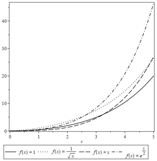
Figure 1. ${}^f\mathrm{Zi}_{-{\displaystyle \frac{1}{4}},{\displaystyle \frac{1}{4}}}\left(x\right)$ for different values of f(x).

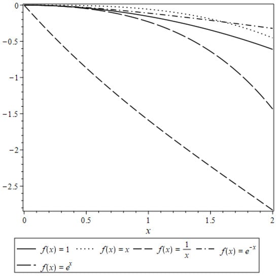
Figure 2. ${}^f\mathrm{Zi}_{-{\displaystyle \frac{1}{2}},{\displaystyle \frac{-1}{4}}}\left(x\right)$ for different values of f(x).

4. Derivatives of the Function ${}^{\mathit{f}}\mathrm{Zi}_{\mathbf{\kappa },\mathit{\mu }}\left(\mathit{x}\right)$

The derivatives of the Whittaker functions are given in [2] as

$${\mathrm{M}}_{\kappa ,\mu }^{\prime }\left(x\right)=\left({\displaystyle \frac{1}{2}}-{\displaystyle \frac{\kappa }{x}}\right){\mathrm{M}}_{\kappa ,\mu }\left(x\right)+\left({\displaystyle \frac{1}{2}}+\mu +\kappa \right){\displaystyle \frac{{\mathrm{M}}_{\kappa +1,\mu }\left(x\right)}{x}},$$

(59)

$${\mathrm{W}}_{\kappa ,\mu }^{\prime }\left(x\right)=\left({\displaystyle \frac{1}{2}}-{\displaystyle \frac{\kappa }{x}}\right){\mathrm{W}}_{\kappa ,\mu }\left(x\right)-{\displaystyle \frac{{\mathrm{W}}_{\kappa +1,\mu }\left(x\right)}{x}}.$$

(60)

The derivative of the function ${}^{f}Z_{\kappa ,\mu }\left(x\right)$ is equal to

$${}^{f}Z_{\kappa ,\mu }^{\prime }\left(z\right)=M_{\kappa ,\mu }^{\prime }\left(z\right){}^f\mathrm{Wi}_{\kappa ,\mu }\left(z\right)-W_{\kappa ,\mu }{\left(z\right)}^{\prime }{}^f\mathrm{Mi}_{\kappa ,\mu }\left(z\right).$$

(61)

Using Equations (59) and (60) in (61), we reach the following form of the derivative of the function ${}^{f}Z_{\kappa ,\mu }\left(z\right)$:

$$\begin{array}{cc}\hfill {}^{f}Z_{\kappa ,\mu }^{\prime }\left(x\right)& =\left[\left({\displaystyle \frac{1}{2}}-{\displaystyle \frac{\kappa }{x}}\right){\mathrm{M}}_{\kappa ,\mu }\left(x\right)+\left({\displaystyle \frac{1}{2}}+\mu +\kappa \right){\displaystyle \frac{{\mathrm{M}}_{\kappa +1,\mu }\left(x\right)}{x}}\right]{}^f\mathrm{Wi}_{\kappa ,\mu }\left(x\right)\hfill \\ \hfill & -\left[\left({\displaystyle \frac{1}{2}}-{\displaystyle \frac{\kappa }{x}}\right){\mathrm{W}}_{\kappa ,\mu }\left(x\right)-{\displaystyle \frac{{\mathrm{W}}_{\kappa +1,\mu }\left(x\right)}{x}}\right]{}^f\mathrm{Mi}_{\kappa ,\mu }\left(x\right).\hfill \end{array}$$

(62)

5. Initial and Boundary Value Problems

In this section, we explore examples of initial and boundary value problems related to the inhomogeneous Whittaker equation. To compute the solutions efficiently, we will employ Maple for the necessary calculations and provide the corresponding graphical representations. By doing so, we aim to illustrate the behavior of the solutions under various conditions and gain insights into the underlying mathematical structures of the equation.

5.1. Initial Value Problems

Theorem 2.

Consider the inhomogeneous Whittaker Equation (11) with the initial conditions:

$$W\left(a\right)=\alpha ;W^{\prime }\left(a\right)=\beta ,$$

(63)

where α and β are known constants. Then, the solution to the initial value problem is given by

$$W\left(x\right)=C_1{\mathrm{M}}_{\kappa ,\mu }\left(x\right)+C_2{\mathrm{W}}_{\kappa ,\mu }\left(x\right)+{\displaystyle \frac{\Gamma \left(\frac{1}{2}+\mu -\kappa \right)}{\Gamma (1+2\mu )}}{}^f\mathrm{Zi}_{\kappa ,\mu }\left(x\right),$$

(64)

where

$$\begin{array}{cc}\hfill C_1={\displaystyle \frac{\Gamma \left(\frac{1}{2}+\mu -\kappa \right)}{\Gamma (1+2\mu )}}[& {\mathrm{W}}_{\kappa ,\mu }\left(a\right)\left(\beta -{\displaystyle \frac{\Gamma \left(\frac{1}{2}+\mu -\kappa \right)}{\Gamma (1+2\mu )}}{}^f\mathrm{Zi}_{\kappa ,\mu }^{\prime }\left(a\right)\right)\hfill \\ \hfill -& {\mathrm{W}}_{\kappa ,\mu }^{\prime }\left(a\right)\left(\alpha -{\displaystyle \frac{\Gamma \left(\frac{1}{2}+\mu -\kappa \right)}{\Gamma (1+2\mu )}}{}^f\mathrm{Zi}_{\kappa ,\mu }\left(a\right)\right)]\hfill \end{array}$$

(65)

and

$$\begin{array}{cc}\hfill C_2={\displaystyle \frac{\Gamma \left(\frac{1}{2}+\mu -\kappa \right)}{\Gamma (1+2\mu )}}[& {\mathrm{M}}_{\kappa ,\mu }^{\prime }\left(a\right)\left(\alpha -{\displaystyle \frac{\Gamma \left(\frac{1}{2}+\mu -\kappa \right)}{\Gamma (1+2\mu )}}{}^f\mathrm{Zi}_{\kappa ,\mu }\left(a\right)\right)\hfill \\ \hfill -& {\mathrm{M}}_{\kappa ,\mu }\left(a\right)\left(\beta -{\displaystyle \frac{\Gamma \left(\frac{1}{2}+\mu -\kappa \right)}{\Gamma (1+2\mu )}}{}^f\mathrm{Zi}_{\kappa ,\mu }^{\prime }\left(a\right)\right)].\hfill \end{array}$$

(66)

Proof. 

By applying the initial conditions (63) in (19), we obtain

$$\begin{array}{cc}\hfill & C_1{\mathrm{M}}_{\kappa ,\mu }\left(a\right)+C_2{\mathrm{W}}_{\kappa ,\mu }\left(a\right)+{\displaystyle \frac{\Gamma \left(\frac{1}{2}+\mu -\kappa \right)}{\Gamma (1+2\mu )}}{}^f\mathrm{Zi}_{\kappa ,\mu }\left(a\right)=\alpha ,\hfill \\ \hfill & C_1{\mathrm{M}}_{\kappa ,\mu }^{\prime }\left(a\right)+C_2{\mathrm{W}}_{\kappa ,\mu }^{\prime }\left(a\right)+{\displaystyle \frac{\Gamma \left(\frac{1}{2}+\mu -\kappa \right)}{\Gamma (1+2\mu )}}{}^f\mathrm{Zi}_{\kappa ,\mu }^{\prime }\left(a\right)=\beta ,\hfill \end{array}$$

(67)

which can be rewritten in matrix form as

$$\left[\begin{array}{cc}{\mathrm{M}}_{k,\mu }\left(a\right)\hfill & {\mathrm{W}}_{k,\mu }\left(a\right)\hfill \\ {\mathrm{M}}_{k,\mu }^{\prime }\left(a\right)\hfill & {\mathrm{W}}_{k,\mu }^{\prime }\left(a\right)\hfill \end{array}\right]\left[\begin{array}{c}{C}_1\hfill \\ C_2\hfill \end{array}\right]=\left[\begin{array}{c}\alpha -{\displaystyle \frac{\Gamma \left(\frac{1}{2}+\mu -\kappa \right)}{\Gamma (1+2\mu )}}{}^f\mathrm{Zi}_{\kappa ,\mu }\left(a\right)\hfill \\ \beta -{\displaystyle \frac{\Gamma \left(\frac{1}{2}+\mu -\kappa \right)}{\Gamma (1+2\mu )}}{}^f\mathrm{Zi}_{\kappa ,\mu }^{\prime }\left(a\right)\hfill \end{array}\right].$$

(68)

Upon solving the system, we obtain

$$\begin{array}{cc}\hfill C_1={\displaystyle \frac{\Gamma \left(\frac{1}{2}+\mu -\kappa \right)}{\Gamma (1+2\mu )}}[& {\mathrm{W}}_{\kappa ,\mu }\left(a\right)\left(\beta -{\displaystyle \frac{\Gamma \left(\frac{1}{2}+\mu -\kappa \right)}{\Gamma (1+2\mu )}}{}^f\mathrm{Zi}_{\kappa ,\mu }^{\prime }\left(a\right)\right)\hfill \\ \hfill -& {\mathrm{W}}_{\kappa ,\mu }^{\prime }\left(a\right)\left(\alpha -{\displaystyle \frac{\Gamma \left(\frac{1}{2}+\mu -\kappa \right)}{\Gamma (1+2\mu )}}{}^f\mathrm{Zi}_{\kappa ,\mu }\left(a\right)\right)],\hfill \end{array}$$

(69)

$$\begin{array}{cc}\hfill C_2={\displaystyle \frac{\Gamma \left(\frac{1}{2}+\mu -\kappa \right)}{\Gamma (1+2\mu )}}[& {\mathrm{M}}_{\kappa ,\mu }^{\prime }\left(a\right)\left(\alpha -{\displaystyle \frac{\Gamma \left(\frac{1}{2}+\mu -\kappa \right)}{\Gamma (1+2\mu )}}{}^f\mathrm{Zi}_{\kappa ,\mu }\left(a\right)\right)\hfill \\ \hfill -& {\mathrm{M}}_{\kappa ,\mu }\left(a\right)\left(\beta -{\displaystyle \frac{\Gamma \left(\frac{1}{2}+\mu -\kappa \right)}{\Gamma (1+2\mu )}}{}^f\mathrm{Zi}_{\kappa ,\mu }^{\prime }\left(a\right)\right)]\hfill \end{array}$$

(70)

□

Since ${}^f\mathrm{Zi}_{\kappa ,\mu }\left(0\right)={}^f\mathrm{Zi}_{\kappa ,\mu }^{\prime }\left(0\right)=0$, the values of the constants $C_1$ and $C_2$ in case $a=0$ are

$$C_1={\displaystyle \frac{\Gamma \left(\frac{1}{2}+\mu -\kappa \right)}{\Gamma (1+2\mu )}}\left[\beta {\mathrm{W}}_{k,\mu }\left(0\right)-\alpha {\mathrm{W}}_{k,\mu }^{\prime }\left(0\right)\right],$$

(71)

$$C_2={\displaystyle \frac{\Gamma \left(\frac{1}{2}+\mu -\kappa \right)}{\Gamma (1+2\mu )}}\left[\alpha {\mathrm{M}}_{k,\mu }^{\prime }\left(0\right)-\beta {\mathrm{M}}_{k,\mu }\left(0\right)\right].$$

(72)

The limiting behavior of the Whittaker functions for $x\to 0$ and real parameters [2] are

$$\begin{array}{cc}\hfill & {\mathrm{M}}_{\kappa ,\mu }\left(x\right)=x^{\mu +{\displaystyle \frac{1}{2}}}(1+O\left(x\right))\hfill \\ \hfill & 2\mu \ne -1,-2,-3,\dots ,\hfill \end{array}$$

(73)

$$\begin{array}{cc}{\mathrm{W}}_{\kappa ,\mu }\left(x\right)={\displaystyle \frac{\Gamma \left(2\mu \right)}{\Gamma \left(\frac{1}{2}+\mu -\kappa \right)}}{x}^{{\displaystyle \frac{1}{2}}-\mu }+O\left(x^{{\displaystyle \frac{3}{2}}-\mu }\right),& \mu >{\displaystyle \frac{1}{2}},\\ {\mathrm{W}}_{\kappa ,{\displaystyle \frac{1}{2}}}\left(x\right)={\displaystyle \frac{1}{\Gamma (1-\kappa )}}+O(xlnx),& \\ {\mathrm{W}}_{\kappa ,\mu }\left(x\right)={\displaystyle \frac{\Gamma \left(2\mu \right)}{\Gamma \left(\frac{1}{2}+\mu -\kappa \right)}}{x}^{{\displaystyle \frac{1}{2}}-\mu }+{\displaystyle \frac{\Gamma (-2\mu )}{\Gamma \left(\frac{1}{2}-\mu -\kappa \right)}}{x}^{{\displaystyle \frac{1}{2}}+\mu }+O\left(x^{{\displaystyle \frac{3}{2}}-\mu }\right),& 0<\mu <{\displaystyle \frac{1}{2}},\\ {\mathrm{W}}_{\kappa ,0}\left(x\right)=-{\displaystyle \frac{\sqrt{x}}{\Gamma \left(\frac{1}{2}-\kappa \right)}}\left(lnx+\psi \left({\displaystyle \frac{1}{2}}-\kappa \right)+2\gamma \right)+O\left(x^{3/2}lnx\right),\end{array}$$

(74)

where, $\psi \left(z\right)$ is given by

$$\begin{array}{cc}\hfill & \psi \left(x\right)={\Gamma }^{\prime }\left(x\right)/\Gamma \left(x\right),\hfill \\ \hfill & x\ne 0,-1,-2,\dots .\hfill \end{array}$$

(75)

The solution of the initial value problem is shown in in Figure 3 for various $f\left(x\right)$. It should be emphasized that all numerical results presented in the figures were obtained through the application of the function ${}^f\mathrm{Zi}_{\kappa ,\mu }\left(x\right)$, in conjunction with Theorem 2.

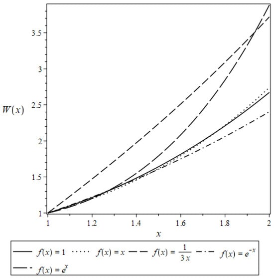
Figure 3. Solution of ${\displaystyle \frac{{\mathrm{d}}^2}{\mathrm{d}{x}^2}}W\left(x\right)+\left(-{\displaystyle \frac{1}{4}}-{\displaystyle \frac{1}{4x}}+{\displaystyle \frac{3}{16x^2}}\right)W\left(x\right)=f\left(x\right),W\left(1\right)=1,W^{\prime }\left(1\right)=1$ for different values of $f\left(x\right)$.

5.2. Boundary Value Problems

In the previous section, we derived the solution to the inhomogeneous Whittaker equation under a set of prescribed initial conditions. This formulation allowed us to explore the time-evolution and dynamic behavior of the system starting from known initial states. The focus was primarily on the temporal aspect of the solution, assuming the spatial domain and boundary influences were either trivial or not the primary concern.

In the present section, we shift our attention to a more general and practically significant case: the solution of the inhomogeneous Whittaker equation subject to boundary conditions. This framework is especially pertinent to physical systems in which spatial boundary behavior significantly influences the overall dynamics, such as quantum mechanical potential problems, heat conduction processes, fluid flow through porous media, and wave propagation in confined or bounded domains. To this end, we consider the inhomogeneous Whittaker Equation (11) subject to the following boundary conditions:

$$W\left(a\right)=\alpha ;W\left(b\right)=\beta ,$$

(76)

where $\alpha$ and $\beta$ are known constants.

Theorem 3.

Consider the inhomogeneous Whittaker equation given by (11) subject to the boundary conditions

$$W\left(a\right)=\alpha ,W\left(b\right)=\beta ,$$

(77)

where $\alpha ,\beta$ are prescribed constants.

Then, the solution to the boundary value problem is given by

$$W\left(x\right)=C_1{\mathrm{M}}_{\kappa ,\mu }\left(x\right)+C_2{\mathrm{W}}_{\kappa ,\mu }\left(x\right)+{\displaystyle \frac{\Gamma \left(\frac{1}{2}+\mu -\kappa \right)}{\Gamma (1+2\mu )}}{}^f\mathrm{Zi}_{\kappa ,\mu }\left(x\right),$$

(78)

where

$$\begin{array}{cc}\hfill C_1={\displaystyle \frac{1}{{\mathrm{M}}_{\kappa ,\mu }\left(a\right){\mathrm{W}}_{\kappa ,\mu }\left(b\right)-{\mathrm{M}}_{\kappa ,\mu }\left(b\right){\mathrm{W}}_{\kappa ,\mu }\left(a\right)}}[& {\mathrm{W}}_{\kappa ,\mu }\left(b\right)\left(\alpha -{\displaystyle \frac{\Gamma \left(\frac{1}{2}+\mu -\kappa \right)}{\Gamma (1+2\mu )}}{\mathrm{Zi}}_{\kappa ,\mu }\left(a\right)\right)\hfill \\ \hfill -& {\mathrm{W}}_{\kappa ,\mu }\left(a\right)\left(\beta -{\displaystyle \frac{\Gamma \left(\frac{1}{2}+\mu -\kappa \right)}{\Gamma (1+2\mu )}}{\mathrm{Zi}}_{\kappa ,\mu }\left(b\right)\right)],\hfill \end{array}$$

(79)

$$\begin{array}{cc}\hfill C_2={\displaystyle \frac{1}{{\mathrm{M}}_{\kappa ,\mu }\left(a\right){\mathrm{W}}_{\kappa ,\mu }\left(b\right)-{\mathrm{M}}_{\kappa ,\mu }\left(b\right){\mathrm{W}}_{\kappa ,\mu }\left(a\right)}}[& {\mathrm{M}}_{\kappa ,\mu }\left(a\right)\left(\beta -{\displaystyle \frac{\Gamma \left(\frac{1}{2}+\mu -\kappa \right)}{\Gamma (1+2\mu )}}{\mathrm{Zi}}_{\kappa ,\mu }\left(b\right)\right)\hfill \\ \hfill -& {\mathrm{M}}_{\kappa ,\mu }\left(b\right)\left(\alpha -{\displaystyle \frac{\Gamma \left(\frac{1}{2}+\mu -\kappa \right)}{\Gamma (1+2\mu )}}{\mathrm{Zi}}_{\kappa ,\mu }\left(a\right)\right)].\hfill \end{array}$$

(80)

Proof. 

Applying the boundary conditions (77) in (19), we obtain

$$\begin{array}{cc}\hfill & C_1{\mathrm{M}}_{\kappa ,\mu }\left(a\right)+C_2{\mathrm{W}}_{\kappa ,\mu }\left(a\right)+{\displaystyle \frac{\Gamma \left(\frac{1}{2}+\mu -\kappa \right)}{\Gamma (1+2\mu )}}{}^f\mathrm{Zi}_{\kappa ,\mu }\left(a\right)=\alpha ,\hfill \\ \hfill & C_1{\mathrm{M}}_{\kappa ,\mu }\left(b\right)+C_2{\mathrm{W}}_{\kappa ,\mu }\left(b\right)+{\displaystyle \frac{\Gamma \left(\frac{1}{2}+\mu -\kappa \right)}{\Gamma (1+2\mu )}}{}^f\mathrm{Zi}_{\kappa ,\mu }\left(b\right)=\beta .\hfill \end{array}$$

(81)

The equations in (81) can be rewritten in matrix form as

$$\left[\begin{array}{cc}{\mathrm{M}}_{k,\mu }\left(a\right)\hfill & {\mathrm{W}}_{k,\mu }\left(a\right)\hfill \\ {\mathrm{M}}_{k,\mu }\left(b\right)\hfill & {\mathrm{W}}_{k,\mu }\left(b\right)\hfill \end{array}\right]\left[\begin{array}{c}{C}_1\hfill \\ C_2\hfill \end{array}\right]=\left[\begin{array}{c}\alpha -{\displaystyle \frac{\Gamma \left(\frac{1}{2}+\mu -\kappa \right)}{\Gamma (1+2\mu )}}{}^f\mathrm{Zi}_{\kappa ,\mu }\left(a\right)\hfill \\ \beta -{\displaystyle \frac{\Gamma \left(\frac{1}{2}+\mu -\kappa \right)}{\Gamma (1+2\mu )}}{}^f\mathrm{Zi}_{\kappa ,\mu }\left(b\right)\hfill \end{array}\right].$$

(82)

Upon solving the system, we obtain

$$\begin{array}{cc}\hfill C_1={\displaystyle \frac{1}{{\mathrm{M}}_{\kappa ,\mu }\left(a\right){\mathrm{W}}_{\kappa ,\mu }\left(b\right)-{\mathrm{M}}_{\kappa ,\mu }\left(b\right){\mathrm{W}}_{\kappa ,\mu }\left(a\right)}}[& {\mathrm{W}}_{\kappa ,\mu }\left(b\right)\left(\alpha -{\displaystyle \frac{\Gamma \left(\frac{1}{2}+\mu -\kappa \right)}{\Gamma (1+2\mu )}}{\mathrm{Zi}}_{\kappa ,\mu }\left(a\right)\right)\hfill \\ \hfill -& {\mathrm{W}}_{\kappa ,\mu }\left(a\right)\left(\beta -{\displaystyle \frac{\Gamma \left(\frac{1}{2}+\mu -\kappa \right)}{\Gamma (1+2\mu )}}{\mathrm{Zi}}_{\kappa ,\mu }\left(b\right)\right)]\hfill \end{array}$$

(83)

and

$$\begin{array}{cc}\hfill C_2={\displaystyle \frac{1}{{\mathrm{M}}_{\kappa ,\mu }\left(a\right){\mathrm{W}}_{\kappa ,\mu }\left(b\right)-{\mathrm{M}}_{\kappa ,\mu }\left(b\right){\mathrm{W}}_{\kappa ,\mu }\left(a\right)}}[& {\mathrm{M}}_{\kappa ,\mu }\left(a\right)\left(\beta -{\displaystyle \frac{\Gamma \left(\frac{1}{2}+\mu -\kappa \right)}{\Gamma (1+2\mu )}}{\mathrm{Zi}}_{\kappa ,\mu }\left(b\right)\right)\hfill \\ \hfill -& {\mathrm{M}}_{\kappa ,\mu }\left(b\right)\left(\alpha -{\displaystyle \frac{\Gamma \left(\frac{1}{2}+\mu -\kappa \right)}{\Gamma (1+2\mu )}}{\mathrm{Zi}}_{\kappa ,\mu }\left(a\right)\right)].\hfill \end{array}$$

(84)

□

Figure 4 shows the solution of the inhomogeneous Whittaker equation for $\kappa =-{\displaystyle \frac{1}{4}}$ and $\mu ={\displaystyle \frac{1}{4}}$ with boundary conditions.

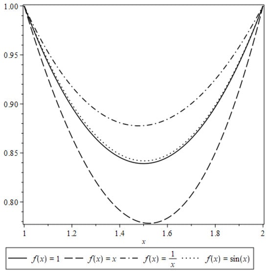
Figure 4. Solution of ${\displaystyle \frac{{\mathrm{d}}^2}{\mathrm{d}{x}^2}}W\left(x\right)+\left(-{\displaystyle \frac{1}{4}}-{\displaystyle \frac{1}{4x}}+{\displaystyle \frac{3}{16x^2}}\right)W\left(x\right)=f\left(x\right),W\left(1\right)=1,W\left(2\right)=1$ for different values of $f\left(x\right)$.

Figure 5 illustrates the behavior of the solution to the boundary value problem near zero.

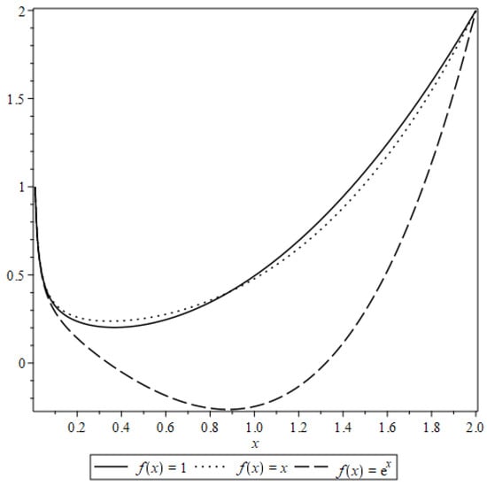
Figure 5. Solution of ${\displaystyle \frac{{\mathrm{d}}^2}{\mathrm{d}{x}^2}}W\left(x\right)+\left(-{\displaystyle \frac{1}{4}}-{\displaystyle \frac{1}{2x}}-{\displaystyle \frac{3}{4x^2}}\right)W\left(x\right)=f\left(x\right),W\left(0.01\right)=1,W\left(2\right)=2$ for different values of $f\left(x\right)$.

6. Conclusions

The primary objective of this work has been to develop a method for solving the inhomogeneous Whittaker differential equation. To achieve this, we introduced a novel class of special integral functions, denoted by ${}^f\mathrm{Zi}_{\kappa ,\mu }\left(a\right)$, which facilitate the construction of particular solutions to the inhomogeneous form of the Whittaker equation. A detailed analytical study of the function ${}^f\mathrm{Zi}_{\kappa ,\mu }\left(a\right)$ was carried out, including the investigation of its fundamental properties and the derivation of expressions for its derivatives. Computational formulas were established for certain representative cases, especially when the forcing function $f\left(x\right)$ and the associated parameters $\kappa$ and $\mu$ take specific, analytically tractable forms.

To complement the theoretical analysis, we provided graphical representations of the function ${}^f\mathrm{Zi}_{\kappa ,\mu }\left(a\right)$, which reveal its behavior under various parameter regimes. These visualizations not only illustrate the properties of the ${}^f\mathrm{Zi}_{\kappa ,\mu }\left(a\right)$ function but also highlight the structure of the corresponding solutions to initial and boundary value problems associated with the Whittaker inhomogeneous differential equation.

The results presented in this work contribute to the broader understanding of special function theory in the context of linear differential equations with inhomogeneous terms. The approach developed here opens up further avenues for the study of related differential systems and may serve as a foundation for applications in mathematical physics and engineering where such equations naturally arise.

References

- Whittaker, E. An expression of certain known functions as generalized hypergeometric functions. Bull. Am. Math. Soc. 1903, 10, 125–134. [Google Scholar] [CrossRef]
- Olver, F.; Lozier, D.; Boisvert, R.; Clark, C. NIST Handbook of Mathematical Functions; Cambridge University Press: Cambridge, UK, 2010. [Google Scholar]
- Abu Zaytoon, M.S.; Alderson, T.L.; Hamdan, M.H. Weber’s inhomogeneous differential equation with initial and boundary con-ditions. Int. J. Open Problems Compt. Math. 2016, 9, 1–11. [Google Scholar] [CrossRef]
- Abu Zaytoon, M.S.; Hamdan, M.H. Weber equation model of flow through a variable-permeability porous core bounded by fluid layers. J. Fluids Eng. Trans. ASME 2022, 144, 041302. [Google Scholar] [CrossRef]
- Hochstadt, H. The Functions of Mathematical Physics; John Wiley & Sons, Inc.: New York, NY, USA, 1971. [Google Scholar]
- Gaspard, D. Connection formulas between Coulomb wave functions. J. Math. Phys. 2018, 59, 112104. [Google Scholar] [CrossRef]
- Akbarzadeh, P. A new exact-analytical solution for convective heat transfer of nanofluids flow in isothermal pipes. J. Mech. 2017, 35, 233–242. [Google Scholar] [CrossRef]
- Gupta, S.; Bhengra, N. Dispersion study of propagation of torsional surface wave in a layered structure. J. Mech. 2017, 33, 303–315. [Google Scholar] [CrossRef]
- Conway, J.T. Indefinite integrals from Wronskians for Whittaker and Gauss hypergeometric functions. Integral Transform. Spec. Funct. 2022, 33, 609–622. [Google Scholar] [CrossRef]
- Abramowitz, M.; Stegun, I.A. Handbook of Mathematical Functions; Dover: New York, NY, USA, 1984. [Google Scholar]
- Magnus, W.; Oberhettinger, F.; Soni, R. Formulas and Theorems for the Special Functions of Mathematical Physics, 3rd ed.; Springer: Berlin/Heidelberg, Germany, 1966. [Google Scholar]
- Mainardi, F.; Paris, R.B.; Consiglio, A. Wright functions of the second kind and Whittaker functions. Fract. Calc. Appl. Anal. 2022, 25, 858–875. [Google Scholar] [CrossRef]
- Szmytkowski, R.; Bielski, S. An orthogonality relation for the Whittaker functions of the second kind of imaginary order. Integral Transform. Spec. Funct. 2010, 21, 739–744. [Google Scholar] [CrossRef]
- Chang, C.-C.; Chu, B.-T.; O’Brien, V. Asymptotic expansion of the Whittaker’s function Wk,m(z) for large values of k,m,z. J. Frankl. Inst. 1953, 255, 215–236. [Google Scholar] [CrossRef]
- Dunster, T.M. Uniform asymptotic expansions for the Whittaker functions Mκ,μ(z) and Wκ,μ(z) with μ large. Proc. Roy. Soc. London A 2021, 477, 20210360. [Google Scholar]
- Izarra, C.; Vallée, O.; Picart, J.; Minh, N.T. Computation of the Whittaker functions Wκ,μ(z) with series expansions and Padé Approximants. Comput. Phys. 1995, 9, 318–323. [Google Scholar] [CrossRef]
- Ragab, F.M. Integrals involving Whittaker functions. Ann. Di Mat. Pura Ed Appl. 1964, 65, 49–79. [Google Scholar] [CrossRef]
- Slater, L.J. Confluent Hypergeometric Functions; Cambridge University Press: Cambridge, UK, 1960. [Google Scholar]
- Mathews, W.N., Jr.; Esrick, M.A.; Teoh, Z.Y.; Freericks, J.K. A physicist’s guide to the solution of Kummer’s equation and confluent hypergeometric functions. Condens. Matter Phys. 2022, 25, 33203. [Google Scholar] [CrossRef]
- Apelblat, A.; González-Santander, J.L. The integral Mittag-Leffler, Whittaker and Wright functions. Mathematics 2021, 9, 3255. [Google Scholar] [CrossRef]
Disclaimer/Publisher’s Note: The statements, opinions and data contained in all publications are solely those of the individual author(s) and contributor(s) and not of MDPI and/or the editor(s). MDPI and/or the editor(s) disclaim responsibility for any injury to people or property resulting from any ideas, methods, instructions or products referred to in the content. |
© 2025 by the authors. Licensee MDPI, Basel, Switzerland. This article is an open access article distributed under the terms and conditions of the Creative Commons Attribution (CC BY) license (https://creativecommons.org/licenses/by/4.0/).