An Analytic Approximation for the Bessel Function J_ν(x) for −1/2 < ν < 3/2

Abstract

We found analytic approximations for the Bessel function of the first kind $J_{\nu }\left(x\right)$, valid for any real value of x and any value of $\nu$ in the interval (−1/2, 3/2). The present approximation is exact for $\nu =-1/2$, $\nu =1/2$, and $\nu =3/2$, where an exact function for each case is well known. The maximum absolute errors for $\nu$ near these peculiar values are very small. Throughout the interval, the absolute values remain below 0.05. The structure of the approximate function is defined considering the corresponding power series and asymptotic expansions, and they are quotients of three polynomials of the second degree combined with trigonometrical functions and fractional powers. This is, in some way, the Multipoint Quasi-rational Approximation (MPQA) technique, but now only two variables are considered, x and $\nu$, which is novel, since in all previous publications only the variable x was considered and $\nu$ was given. Furthermore, in the case of $J_{-1/2}\left(x\right)$, $J_{1/2}\left(x\right)$, and $J_{3/2}\left(x\right)$, the corresponding exact function was also a condition to be considered and fulfilled. It is important to point out that the zeros of the exact functions and the approximate ones are also almost coincident with small relative errors. Finally, the approximation presented here has the property of preservation of symmetry for $\nu >0$, i.e., when there is a sign change in the variable x, the corresponding change agrees with a similar change in the power series of the exact function.

1. Introduction

Regular Bessel functions $J_{\nu }\left(x\right)$ usually appear in important applications in Physics, Electrodynamics, and Engineering [1,2,3,4,5,6,7], including works that employ $J_0$ to obtain magnetic fields [8], as well as others where both $J_0$ and $J_1$ functions arise; for example, in the modeling of antenna structures [9] and in thermal phenomena of superconducting wires [10]. Their power series and asymptotic expansions are well known [11], and the calculation for small values of the variable x is straightforward. However, the power series converges slowly when x increases, requiring a large number of terms to achieve an acceptable accuracy. On the other hand, the asymptotic expansions are only valid for sufficiently large x, and they lose precision in intermediate ranges. As a result, obtaining reliable numerical values of $J_{\nu }\left(x\right)$ for the values commonly needed in applications is not trivial, and motivates the search for alternative representations and efficient approximation schemes.

In this work, an analytical approximation for the aforementioned functions is presented, valid for any value of the variable x and for orders $\nu$ within the range $-1/2\le \nu \le 3/2$. The technique we used is an extension of the Multipoint Quasirational Approximation (MPQA) method, which has been the subject of several previous works [12,13,14,15,16]. In this case, the accuracy of the approximation is exact for $\nu =-1/2$, $\nu =1/2$, and $\nu =3/2$. Furthermore, the precision remains high for most values of the order $\nu$ within the interval considered.

In the present method, both power series and asymptotic expansions are employed, and rational functions are combined with other elementary functions. This distinguishes the present technique from the Padé approximation, as the rational functions must be combined with other elementary functions due to the use of asymptotic expansions. Consequently, the usual issues associated with Padé approximations [17,18] as the so-called defects (a zero in the denominator with another zero nearby in the numerator) have been avoided in the present work. This paper is organized as follows: theoretical analysis is presented in Section 2, and the results are presented in Section 3. Finally, the last section will be devoted to the conclusions.

2. Theoretical Analysis

The power series of the Regular Bessel functions [11] are given by

$$J_{\nu }\left(x\right)={\left({\displaystyle \frac{x}{2}}\right)}^{\nu }\sum _{k=0}^{\infty }{\displaystyle \frac{{(-1)}^k}{k!\Gamma (k+\nu +1)}}{\left({\displaystyle \frac{x}{2}}\right)}^{2k},$$

(1)

which can also be written as follows:

$$J_{\nu }\left(x\right)={\displaystyle \frac{x^{\nu }}{2^{\nu }\Gamma (\nu +1)}}\left(1-a_1{x}^2+a_2{x}^4-a_3{x}^6+\dots \right)={\displaystyle \frac{1}{\Gamma (\nu +1)}}{\left({\displaystyle \frac{x}{2}}\right)}^{\nu }\sum _{j=0}^{\infty }{(-1)}^j{a}_j{x}^{2j},$$

(2)

where $a_j=1/4^{j}j!{(\nu +1)}_j$, with ${(\nu +1)}_j$ the rising factorial (Pochhammer symbol). Thus, we can express $a_0=1$,

$$\begin{array}{ccc}\hfill a_1& =& {\displaystyle \frac{1}{4(\nu +1)}},\hfill \end{array}$$

(3)

$$\begin{array}{ccc}\hfill a_2& =& {\displaystyle \frac{1}{32(\nu +1)(\nu +2)}},\hfill \end{array}$$

(4)

$$\begin{array}{ccc}\hfill a_3& =& {\displaystyle \frac{1}{384(\nu +1)(\nu +2)(\nu +3)}}.\hfill \end{array}$$

(5)

The corresponding asymptotic expansions of these functions are expressed as follows [11]:

$$J_{\nu }\left(x\right)\sim \sqrt{{\displaystyle \frac{2}{\pi x}}}\left[sin\alpha sinx+cos\alpha cosx+\mathcal{O}(1/x)\right],$$

(6)

where

$$\alpha \left(\nu \right)=(2\nu +1){\displaystyle \frac{\pi }{4}}.$$

(7)

To simplify the notation, the following constants and variables are introduced as follows:

$$\begin{array}{ccc}\hfill a\left(\nu \right)& =& 2^{\nu }\Gamma (\nu +1),\hfill \end{array}$$

(8)

$$\begin{array}{ccc}\hfill \beta \left(\nu \right)& =& {\displaystyle \frac{2\nu -1}{4}},\hfill \\ \hfill \gamma \left(\nu \right)& =& |1-2(\nu -\left[\nu \right]\left)\right|,\hfill \end{array}$$

(9)

$$\begin{array}{ccc}\hfill \chi & =& x-\alpha \left(\nu \right).\hfill \end{array}$$

(10)

where $\left[\nu \right]$ is the integer part of $\nu$. Additionally, it is well-known that

$$\begin{array}{ccc}\hfill J_{-1/2}\left(x\right)& =& \sqrt{{\displaystyle \frac{2}{\pi }}}{\displaystyle \frac{cosx}{\sqrt{\left|x\right|}}},\hfill \end{array}$$

(11)

$$\begin{array}{ccc}\hfill J_{1/2}\left(x\right)& =& \sqrt{{\displaystyle \frac{2}{\pi }}}{\displaystyle \frac{sinx}{\sqrt{\left|x\right|}}},\hfill \end{array}$$

(12)

$$\begin{array}{ccc}\hfill J_{3/2}\left(x\right)& =& \sqrt{{\displaystyle \frac{2}{\pi }}}\left({\displaystyle \frac{sinx}{\sqrt{{\left|x\right|}^3}}}-{\displaystyle \frac{cosx}{\sqrt{\left|x\right|}}}\right).\hfill \end{array}$$

(13)

The bridge approximation function, which connects the power and asymptotic expansions, is constructed as follows:

$${\tilde{J}}_{\nu }\left(x\right)={\displaystyle \frac{x^{\nu -1}\left[(p_0+{\tilde{p}}_0\sqrt{1+{\gamma }^4{x}^2}+p_2{x}^2)sinx+(p_1+p_3\sqrt{1+{\gamma }^4{x}^2})xcosx\right]}{a{(1+{\gamma }^4{x}^2)}^{\beta }(q_0+x^2)}}.$$

(14)

To explain the derivation of this structure, the following points are highlighted:

1.

From the power series, it is evident that the approximation must include only the even powers of the variable x, in order to preserve the symmetry.

2.

The asymptotic behavior indicates that the approximation should incorporate $sinx$ and $cosx$ combined with $x^{-1/2}$. This is achieved because the power term $p_2{x}^2$ is compensated for by $q_0+x^2$, and the factor $x^{\nu -1}$ simplifies with $2\beta$, resulting in the required $x^{-1/2}$. For $cosx$, the additional power of x is taken into account for the numerator function, to preserve symmetry.

3.

From the power series, it is known that $x^{\nu }$ is multiplied by even power series. This property is also presented in the approximate function ${\tilde{J}}_{\nu }\left(x\right)$.

4.

The approximation must reproduce the exact forms of $J_{1/2}\left(x\right)$ and $J_{3/2}\left(x\right)$ when the parameters are appropriately determined. To ensure this, the term involving $\beta \left(\nu \right)$, must reduce to unity, as happens because $\beta (1/2)=0$ and $\gamma (1/2)=\gamma (3/2)=0$.

The next step involves determining the parameters $p_0$, ${\tilde{p}}_0$, $p_1$, $p_2$, $p_3$, and $q_0$ using the power series and asymptotic expansions. It is worth noting that to avoid complications, the parameters are determined through linear equations, bypassing the challenges of nonlinear relationships. This is achieved by first multiplying the power series of $J_{\nu }\left(x\right)$ by $(q_0+x^2){(1+{\gamma }^4{x}^2)}^{\beta }$, and then equating terms.

From the above, six linear equations are obtained for the parameters $p_0$, ${\tilde{p}}_0$, $p_1$, $p_2$, $p_3$, and $q_0$. Consequently, there are six parameters and six equations. Thus, it is possible to determine all $J_{\nu }\left(x\right)$ and to compute the maximum absolute errors as follows:

$${\epsilon }_{A,\max }=max\left|J_{\nu }\left(x\right)-{\tilde{J}}_{\nu }\left(x\right)\right|.$$

(15)

Relative errors cannot be computed for the entire range of x in this case, since the functions $J_{\nu }\left(x\right)$ have zeros. However, we present an example of its behavior in Appendix B.

In this work, four equations are obtained from the power series and two from the asymptotic expansions. The expansions used for the power series are

$$\begin{array}{ccc}& & {(1+{\gamma }^4{x}^2)}^{\beta }(q_0+x^2)\left(1-a_1{x}^2+a_2{x}^4-a_3{x}^6\pm \dots \right)\hfill \\ & & =\left(p_0+{\tilde{p}}_0\sqrt{1+{\gamma }^4{x}^2}+p_2{x}^2\right){\displaystyle \frac{sinx}{x}}+\left(p_1+p_3\sqrt{1+{\gamma }^4{x}^2}\right)cosx.\hfill \end{array}$$

(16)

which are combined with the additional power series

$$\begin{array}{ccc}\hfill {\left(1+{\gamma }^4{x}^2\right)}^{1/2}& =& 1+{\displaystyle \frac{1}{2}}{\gamma }^4{x}^2-{\displaystyle \frac{1}{8}}{\gamma }^8{x}^4+{\displaystyle \frac{1}{16}}{\gamma }^{12}{x}^6\pm \dots ,\hfill \end{array}$$

(17)

$$\begin{array}{ccc}\hfill {\left(1+{\gamma }^4{x}^2\right)}^{\beta }& =& 1+\beta {\gamma }^4{x}^2+{\displaystyle \frac{1}{2}}\beta (\beta -1){\gamma }^8{x}^4+{\displaystyle \frac{1}{6}}\beta (\beta -1)(\beta -2){\gamma }^{12}{x}^6+\dots ,\hfill \end{array}$$

(18)

$$\begin{array}{ccc}\hfill sinx& =& x-{\displaystyle \frac{1}{6}}{x}^3+{\displaystyle \frac{1}{120}}{x}^5-{\displaystyle \frac{1}{5040}}{x}^7\pm \dots ,\hfill \end{array}$$

(19)

$$\begin{array}{ccc}\hfill cosx& =& 1-{\displaystyle \frac{1}{2}}{x}^2+{\displaystyle \frac{1}{12}}{x}^4-{\displaystyle \frac{1}{720}}{x}^6\pm \dots .\hfill \end{array}$$

(20)

In this way, the following four equations for the parameters are obtained:

$$q_0=p_0+{\tilde{p}}_0+p_1+p_3,$$

(21)

$$1+q_0\beta {\gamma }^4-q_0{a}_1={\displaystyle \frac{1}{6}}\left[-p_0-{\tilde{p}}_0-3(p_1-2p_2+p_3)+3({\tilde{p}}_0+p_3){\gamma }^4\right].$$

(22)

$$\begin{array}{ccc}& & {\displaystyle \frac{15}{4}}\left(16q_0{\beta }^2{\gamma }^8+8\beta {\gamma }^4\left(4-2q_0{\gamma }^4-4q_0{a}_1\right)+32\left(q_0{a}_2-{\displaystyle \frac{1}{4}}\right)\right)\hfill \\ & & =p_0+{\tilde{p}}_0+5(p_1-4p_2+p_3)-10({\tilde{p}}_0+3p_3){\gamma }^4-15({\tilde{p}}_0+p_3){\gamma }^8,\hfill \end{array}$$

(23)

$$\begin{array}{ccc}& & 192(\beta -1)\beta {\gamma }^8+64q_0(\beta -2)(\beta -1)\beta {\gamma }^{12}-192\beta {\gamma }^4{a}_1(2+q_0(\beta -1){\gamma }^4)\hfill \\ & & +384a_2(1+q_0\beta {\gamma }^4)-384q_0{a}_3\hfill \\ & & ={\displaystyle \frac{-p_0-{\tilde{p}}_0-7(p_1-6p_2+p_3)+21({\tilde{p}}_0+5p_3){\gamma }^4+105({\tilde{p}}_0+3p_3){\gamma }^8+315({\tilde{p}}_0+p_3){\gamma }^{12}}{8/105}}.\hfill \end{array}$$

(24)

Two additional equations are obtained from the asymptotical expansions [details are given in Appendix A].

$$\begin{array}{ccc}\hfill p_2& =& \sqrt{{\displaystyle \frac{2}{\pi }}}a{\gamma }^{4\beta }sin\left(\alpha \right),\hfill \end{array}$$

(25)

$$\begin{array}{ccc}\hfill p_3& =& \sqrt{{\displaystyle \frac{2}{\pi }}}a{\gamma }^{4(\beta -1/2)}cos\left(\alpha \right).\hfill \end{array}$$

(26)

In this way six equations are obtained for the six parameters $p_0$, ${\tilde{p}}_0$, $p_1$, $p_2$, $p_3$, and $q_0$.

3. Results

From the previous equations all the parameters are determined. The first parameter to determine is $q_0$, obtaining

$$q_0={\displaystyle \frac{N_0}{D}},$$

(27)

where

$$\begin{array}{ccc}& & N_0={\displaystyle \frac{2^{3/2}{\gamma }^{2+4\beta }a\left((16-525{\gamma }^8)cos\left(\alpha \right)-20{\gamma }^2(4+21{\gamma }^4)sin\left(\alpha \right)\right)}{\sqrt{\pi }/3}}\hfill \\ & & -5040(4+15{\gamma }^4)a_2\hfill \\ & & -18\left(4+5{\gamma }^4\left(11+42{\gamma }^4+4\beta \left(4+7{\gamma }^4\left(1+\beta (4+15{\gamma }^4)\right)\right)\right)\right)\hfill \\ & & +20\left(4+7{\gamma }^4\left(5+64\beta +15(1+16\beta ){\gamma }^4\right)\right)a_1.\hfill \end{array}$$

(28)

and

$$\begin{array}{ccc}\hfill D& =& 4+3{\gamma }^4\left(25+24\beta +15\left(7+2\beta (3+8\beta )\right){\gamma }^4+140\beta \left(10+\beta (8\beta -9)\right){\gamma }^8\right.\hfill \\ & & \left.+2100(\beta -1)\beta (2\beta -1){\gamma }^{12}\right)\hfill \\ & & -18\left(4+5{\gamma }^4\left(11+42{\gamma }^4+4\beta \left(4+7{\gamma }^4\left(-27+32\beta +15(-7+8\beta ){\gamma }^4\right)\right)\right)\right)a_1\hfill \\ & & +360\left(4+7{\gamma }^4\left(5+8\beta +15(1+2\beta ){\gamma }^4\right)\right)a_2\hfill \\ & & -5040\left(4+15{\gamma }^4\right)a_3.\hfill \end{array}$$

(29)

An important point about this parameter is that it must be positive to avoid zeros in the denominator, i.e., the so-called defects in the Padé treatments. This condition is verified in Figure 1 for $\nu$ in the interval (−1/2, 3/2), but later $q_0$ becomes negative and the approximation is no longer useful. This is the reason why the present work is restricted to the mentioned interval.

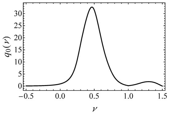
Figure 1. $q_0$ parameter as a function of $\nu$.

The results for the other parameters are given by the following equations:

$$\begin{array}{ccc}& & p_{0}D=\hfill \\ & & 3\sqrt{2}a{\gamma }^{2+4\beta }cos\left(\alpha \right)(16+15{\gamma }^4(11+16\beta +2\left(7+\beta (64\beta -11)\right){\gamma }^4\hfill \\ & & +7(2\beta -1)(15-38\beta +32{\beta }^2){\gamma }^8+210\beta (3+4(\beta -2)\beta ){\gamma }^{12})\hfill \\ & & -30\left(8+{\gamma }^4\left(53+128\beta +84(1+\beta (64\beta -57)){\gamma }^4+105(96{\beta }^2-1-88\beta ){\gamma }^8\right)\right)a_1\hfill \\ & & +120\left(32+21{\gamma }^4(7+16\beta +10(1+3\beta ){\gamma }^4)\right)a_2-5040(8+15{\gamma }^4)a_3)\hfill \\ & & +\sqrt{2}a{\gamma }^{4\beta }sin\left(\alpha \right)(8+3{\gamma }^4(48\beta +15(32(\beta -1)-21\beta ){\gamma }^4\hfill \\ & & +35(2\beta (43+32(\beta -3)\beta )-45){\gamma }^8-6300{\beta }^2{\gamma }^{12}-6300(\beta -1)\beta (2\beta -1){\gamma }^{16})\hfill \\ & & +18\left(5{\gamma }^4\left(-32\beta +7(7-256(-1+\beta )\beta ){\gamma }^4+210(1+2\beta ){\gamma }^8+1260\beta (8\beta -7){\gamma }^{12}\right)-8\right)a_1\hfill \\ & & -360\left(7{\gamma }^4(15{\gamma }^4-16\beta +45(1+2\beta ){\gamma }^8)-8\right)a_2+5040(45{\gamma }^8-8)a_3).\hfill \end{array}$$

(30)

$$\begin{array}{ccc}& & {\tilde{p}}_{0}D=\hfill \\ & & -8\sqrt{2}a{\gamma }^{4\beta }sin\left(\alpha \right)(1+6\beta {\gamma }^4\left(3+10(\beta -1){\gamma }^4(3+14(\beta -2){\gamma }^4)\right)\hfill \\ & & -18\left(1+20\beta {\gamma }^4(1+56(\beta -1){\gamma }^4)\right)a_1+360(1+14\beta {\gamma }^4)a_2-5040a_3)\hfill \\ & & -3\sqrt{2}a{\gamma }^{2+4\beta }cos\left(\alpha \right)(16+5{\gamma }^4(19+21{\gamma }^4+6\beta (8+{\gamma }^4(64\beta -25+14(20+\beta (16\beta -33)){\gamma }^4\hfill \\ & & +70(\beta -1)(2\beta -1){\gamma }^8\left)\right))\hfill \\ & & -30\left(8+{\gamma }^4\left(39+42{\gamma }^4+4\beta \left(32+21{\gamma }^4(64\beta -59+5(8\beta -7){\gamma }^4)\right)\right)\right)a_1\hfill \\ & & +120\left(32+21{\gamma }^4(5+16\beta +5(1+2\beta ){\gamma }^4)\right)a_2-5040(8+5{\gamma }^4)a_3)\hfill \\ & & +6\sqrt{\pi }(1+40\beta {\gamma }^4\left(1+3{\gamma }^4(-2+5\beta +28({\beta }^2-1){\gamma }^4+70\beta ({\beta }^2-1){\gamma }^8)\right)\hfill \\ & & +360\left(1+224\beta {\gamma }^4(1+5(1+\beta ){\gamma }^4)\right)a_1^2+10080a_3\hfill \\ & & -40a_1\left(1+3\beta {\gamma }^4\left(59+42(7+9\beta ){\gamma }^4+280({\beta }^2-1){\gamma }^8\right)+252(1+80\beta {\gamma }^4)a_2+2520a_3\right)\hfill \\ & & +480\left(a_2(1-210\beta {\gamma }^8+210a_2)+210\beta {\gamma }^4{a}_3\right)).\hfill \end{array}$$

(31)

$$\begin{array}{ccc}& & p_{1}D{\gamma }^2=\hfill \\ & & 15\sqrt{2}a{\gamma }^{6+4\beta }sin\left(\alpha \right)(31+21{\gamma }^4\left(7+2\beta \left(7+30{\gamma }^4(\beta +(\beta -1)(2\beta -1){\gamma }^4)\right)\right)\hfill \\ & & -42\left(7+30{\gamma }^4(1+2\beta +6\beta (8\beta -7){\gamma }^4)\right)a_1+2520(1+(3+6\beta ){\gamma }^4)a_2-15120a_3)\hfill \\ & & -\sqrt{2}a{\gamma }^{4\beta }cos\left(\alpha \right)(4+9(21+8\beta ){\gamma }^4+90(7+\beta (17+8\beta )){\gamma }^8\hfill \\ & & +105(-15+4\beta (1+\beta )(1+8\beta )){\gamma }^{12}+9450\beta (3+4(\beta -2)\beta ){\gamma }^{16}\hfill \\ & & -18\left(4+5{\gamma }^4(25+16\beta +28(3+\beta (32\beta -21)){\gamma }^4+105(-1-88\beta +96{\beta }^2){\gamma }^8)\right)a_1\hfill \\ & & +360\left(4+7{\gamma }^4(11+8\beta +30(1+3\beta ){\gamma }^4)\right)a_2-5040(4+45{\gamma }^4)a_3)\hfill \\ & & +3\sqrt{\pi }{\gamma }^2(11+15{\gamma }^4(6+21{\gamma }^4+4\beta (6+7{\gamma }^4(1+10\beta +5(2\beta -1)(5+4\beta ){\gamma }^4\hfill \\ & & +15(1+\beta )(2\beta -1)(1+2\beta ){\gamma }^8\left)\right))\hfill \\ & & +2520\left(1+5{\gamma }^4(1+32\beta +3(1+16\beta (3+2\beta )){\gamma }^4)\right)a_1^2+50400a_3\hfill \\ & & -60a_1(6+7{\gamma }^4\left(5+15{\gamma }^4+2\beta (59+15{\gamma }^4(23+18\beta +(16+\beta (27+8\beta )){\gamma }^4))\right)\hfill \\ & & +420(2+(3+96\beta ){\gamma }^4)a_2+5040a_3)\hfill \\ & & +840\left(a_2(4-45(1+8\beta ){\gamma }^8+360a_2)+90(1+4\beta ){\gamma }^4{a}_3\right)).\hfill \end{array}$$

(32)

Finally, $p_2$ and $p_3$ have already been given in Equations (25) and (26), written here as follows:

$$\begin{array}{ccc}\hfill p_2& =& \sqrt{{\displaystyle \frac{2}{\pi }}}a\left(\nu \right){\gamma }^{4\beta }sin\left[\alpha \left(\nu \right)\right],\hfill \\ \hfill p_3& =& \sqrt{{\displaystyle \frac{2}{\pi }}}a\left(\nu \right){\gamma }^{4(\beta -1/2)}cos\left[\alpha \left(\nu \right)\right].\hfill \end{array}$$

(33)

For some particular values of $\nu$, the parameters are calculated and given in Table 1.

Table 1. Values of the parameters $q_0$, $p_0$, ${\tilde{p}}_0$, $p_1$, $p_2$, and $p_3$, for specific values of $\nu$.

	$\mathit{\nu }=-1/4$	$\mathit{\nu }=0$	$\mathit{\nu }=1/4$	$\mathit{\nu }=3/4$	$\mathit{\nu }=1$
$q_0$	0.188815	0.947332	17.6217	16.9528	0.2080
$p_0$	0.113495	0.703224	17.3098	17.2822	0.2729
${\tilde{p}}_0$	0.00395082	−0.0480095	−2.05988	1.66612	0.556802
$p_1$	−0.112395	−0.272072	0.509957	−0.660611	0.506645
$p_2$	0.171265	0.56419	1.1237	0.805671	1.12838
$p_3$	0.183765	0.56419	1.8618	−1.33488	−1.12838

Now it is clear how each approximate function is determined for each $\nu$, and how to compare it with the exact one. The point is to find the approximate function for the values $\nu =-1/2$, $\nu =1/2$, and $\nu =3/2$. It is clear that $\gamma (-1/2)=2$, $\gamma (1/2)=\gamma (3/2)=0$, and then the complete result is as follows:

$$\begin{array}{ccc}\hfill {\tilde{J}}_{-1/2}\left(x\right)& =& \sqrt{{\displaystyle \frac{2}{\pi }}}{\displaystyle \frac{cosx}{\sqrt{\left|x\right|}}},\hfill \end{array}$$

(34)

$$\begin{array}{ccc}\hfill {\tilde{J}}_{1/2}\left(x\right)& =& \sqrt{{\displaystyle \frac{2}{\pi }}}{\displaystyle \frac{sinx}{\sqrt{\left|x\right|}}},\hfill \end{array}$$

(35)

$$\begin{array}{ccc}\hfill {\tilde{J}}_{3/2}\left(x\right)& =& \sqrt{{\displaystyle \frac{2}{\pi }}}\left({\displaystyle \frac{sinx}{\sqrt{{\left|x\right|}^3}}}-{\displaystyle \frac{cosx}{\sqrt{\left|x\right|}}}\right).\hfill \end{array}$$

(36)

That is, the result is exact.

Another important point is to determine the maximum absolute error for each $\nu$ (the maximum relative errors are always infinity, as was explained in the Section 2). The maximum absolute errors are well defined for $-1/2\le \nu <3/2$. A plot of the maximum absolute errors is shown in Figure 2. From the latter, it is observed that the maximum difference between the exact and approximated function is less than 0.02 in the entire interval.

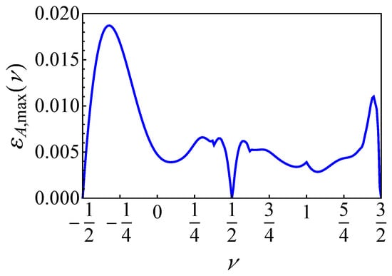
Figure 2. Maximum value of the absolute error obtained as a funcition of $\nu$.

To show the effectiveness of the described technique, let us focus on the details of the results obtained for the orders $\nu =0$ and $\nu =1$. These are shown in the following Figure 3 and Figure 4, respectively. In all cases, the exact and approximate functions are represented by solid and dashed lines, respectively. From the direct comparison, it is clear that the approximated function follows with good accuracy the shape of the exact one, obtaining the value ${\epsilon }_{A,\max }=0.0047$ at $x=3.5591$ for $\nu =0$, and ${\epsilon }_{A,\max }=0.0039$ at $x=3.5383$ for $\nu =1$. Note that a better accuracy between both functions is obtained as x increases.

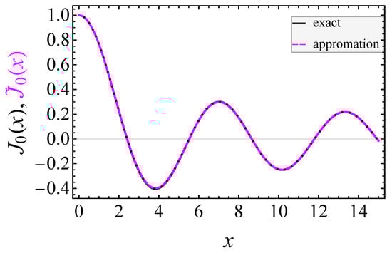
Figure 3. Comparison between the exact and approximated functions for $\nu =0$.

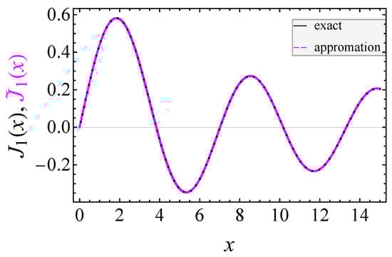
Figure 4. Comparison between the exact and approximated functions for $\nu =1$.

In order to give more details of the accuracy of the results, the relative error for the zeros obtained using the approximated function it is studied. The formula for these relative errors is given by

$${\epsilon }_{\mathrm{rel}}\left(n\right)={\displaystyle \frac{\mid x_n-{\tilde{x}}_n\mid }{x_n}},$$

(37)

where $x_n$ is the n-zero of $J_{\nu }\left(x\right)$ and ${\tilde{x}}_n$ the corresponding one of ${\tilde{J}}_{\nu }\left(x\right)$. The relative errors of the zeros of the Bessel functions for some values of $\nu$ are give in Figure 5.

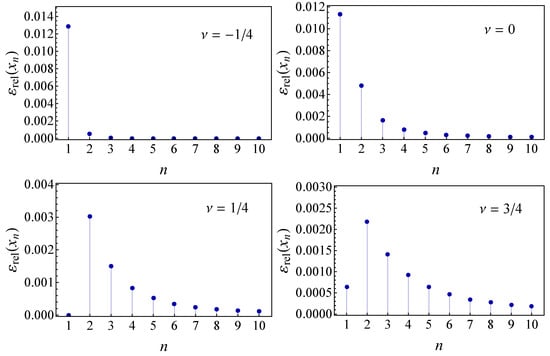
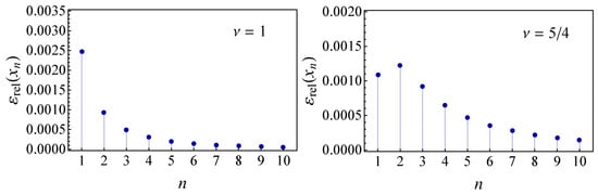
Figure 5. Relative errors in the zeros $x_n$, $n=1,2,3,\dots ,10$. Ten zeros are shown for each of the cases $\nu =-1/4,0,1/4,3/4,1$, and $5/4$.

As it is clear from these graphs (Figure 5), the error decreases always with the increasing of the values of x, for all values of $\nu$.

4. Conclusions

An analytic approximation for the first kind Bessel functions (function $J_{\nu }\left(x\right)$) has been determined for any positive value of the variable x and any value of $\nu$ in the interval $-1/2\le \nu <3/2$. The procedure followed here is novel, as it resembles finding approximations for functions of two variables, although in this case, one of the variables is the order $\nu$ of the Bessel function. The approach employed simultaneously utilizes the power series and the asymptotic expansions of the corresponding functions, as in the Multipoint Quasi-rational Approximation (MPQA) technique. However, the presence of two variables complicates the search for the structure of the approximated function.

The accuracy of the approximations is very good for all the values of $\nu$ inside the considered interval. Furthermore, the approximation coincides with the exact functions in cases where the functions are simpler, such as for $\nu =-1/2$, $\nu =1/2$, and $\nu =3/2$. The maximum errors for each $\nu$ typically occur between integer values of $\nu$ congruents with 1/2. After these points, the errors decrease rapidly. The six parameters of the proposed approximation are determined precisely through six corresponding linear equations. The parameters are not left to be determined via numerical computation, as it is often the case with traditional approximations of the Bessel functions in the interval $-1/2\le \nu <3/2$.

Given the very small errors observed, it appears that the present approximation will be useful for most applications involving the first-kind Bessel functions.

For context, we include a short comparison with Chebyshev-based approximations. These methods perform very well on fixed interval of x and, with rational mappings or by factoring the leading asymptotics, can achieve high accuracy. However, attaining comparable uniform accuracy simultaneously in x and $\nu$ typically requires higher polynomial degree or piecewise expansions. By contrast, the MPQA technique used here enforces both the polinomial series and asymptotics expansions, yielding a single closed form expression that is uniform in x and $\nu$ and has lower evaluation cost [19,20,21,22].

References

- Jackson, J.D. Classical Electrodynamics, 3rd ed.; John Willey and Sons, Inc.: New York, NY, USA, 1998; pp. 112–119. [Google Scholar]
- Watson, G.N. A Treatise on the Theory of Bessel Functions, 2nd ed.; Cambridge University Press: Cambridge, UK, 1966; pp. 85–224. [Google Scholar]
- Rothwell, E.J. Exponential Approximation of the Bessel functions I0(x), I1(x), J0(x), J1(x),Y0(x) and H0(x) with applications to electromagnetic scattering, radiation and diffraction [EM Programmer’s Notebooks]. IEEE Antennas Propag. Mag. 2009, 51, 138–147. [Google Scholar] [CrossRef]
- Khosravian-Arab, H.; Dehghan, M.; Eslahchi, M.R. Generalized Bessel functions: Theory and their applications. Math. Methods Appl. Sci. 2017, 40, 6389–6410. [Google Scholar] [CrossRef]
- Guo, L.; Liang, P. Condensed matter physics in time crystals. New J. Phys. 2020, 22, 075003. [Google Scholar] [CrossRef]
- Ahumada, M.; Valderrama-Quinteros, N.; Romero, G. Floquet-engineered system-reservoir interaction in the transverse field Ising model. arXiv 2025, arXiv:2501.07527. [Google Scholar]
- Chen, K.; Li, J.; Zhu, G.; Zhang, W.; He, Z.; Zheng, G.; Li, Z. Phase-assisted angular-multiplexing nanoprinting based on the Jacobi-Anger expansion. Opt. Express 2022, 30, 46552–46559. [Google Scholar] [CrossRef] [PubMed]
- Collomb, D.; Bending, S.J.; Koshelev, A.E.; Smylie, M.P.; Farrar, L.; Bao, J.-K.; Chung, D.Y.; Kanatzidis, M.G.; Kwok, W.-K.; Welp, U. Observing the Suppression of Superconductivity in RbEuFe4As4 by Correlated Magnetic Fluctuations. Phys. Rev. Lett. 2021, 126, 157001. [Google Scholar] [CrossRef] [PubMed]
- Shaban, M. Development and Implementation of High-Gain, and High-Isolation Multi-Input Multi-Output Antenna for 5G mmWave Communications. Telecom 2025, 6, 14. [Google Scholar] [CrossRef]
- Khan, Z.; Pradhan, S.; Ahmed, I. Temperature Instability in High-Tc Superconducting Wire Exposed to Thermal Disturbance. Procedia Mater. Sci. 2014, 6, 249–255. [Google Scholar] [CrossRef]
- Abramovitz, M.; Stegun, I.A. Handbook of Mathematical Functions; Ninth Printing; Dover Books: New York, NY, USA, 1970; pp. 355–379. [Google Scholar]
- Martin, P.; Castro, E.; Paz, J.L.; De Freitas, A. Chapter 4: Multipoint quasi-rational approximations in Quantum Chemistry. In New Developments in Quantum Chemistry; Paz, J.L., Hernandez, J.A., Eds.; Transworld Research Network: Kerala, India, 2009; Chapter 3; pp. 55–76. [Google Scholar]
- Martin, P.; Ramos-Andrade, J.P.; Caro-Pérez, F.; Lastra, F. Accurate Analytical Approximation for the Bessel Function J2(x). Math. Comput. Appl. 2024, 29, 63. [Google Scholar] [CrossRef]
- Maass, F.; Martin, P.; Olivares, J. Analytic Approximation to the Bessel function J0(x). Comput. Appl. Math. 2020, 39, 222. [Google Scholar] [CrossRef]
- Maass, F.; Martin, P. Precise analytic Approximations for the Bessel function J1(x). Results Phys. 2018, 8, 1234–1238. [Google Scholar] [CrossRef]
- Martin, P.; Rojas, E.; Olivares, J.; Sotomayor, A. Quasi-rational analytic approximation for the modified Bessel function I1(x) with high accuracy. Symmetry 2021, 13, 741–742. [Google Scholar] [CrossRef]
- Baker, G.A., Jr.; Travers-Morris, P. Padé Approximants; Cambrige U.P.: Cambrige, UK, 1996. [Google Scholar]
- Peker, H.A. An Introduction to Padé Approximation. In Current Studies in Basic Sciences, Engineering and Tecnology; ISRES Publishing: Konya, Turkey, 2021; pp. 143–155. [Google Scholar]
- Trefethen, L.N. Approximation Theory and Approximation Practice; SIAM: Philadelphia, PA, USA, 2013. [Google Scholar]
- Boyd, J.P. Orthogonal rational functions on a semi-infinite interval. J. Comput. Phys. 1987, 70, 63–88. [Google Scholar] [CrossRef]
- Gil, A.; Segura, J.; Temme, N.M. Numerical Methods for Special Functions; SIAM: Philadelphia, PA, USA, 2007. [Google Scholar]
- Olver, F.W.J.; Lozier, D.W.; Boisvert, R.F.; Clark, C.W. (Eds.) NIST Handbook of Mathematical Functions; Cambridge University Press: Cambridge, UK, 2010. [Google Scholar]
Disclaimer/Publisher’s Note: The statements, opinions and data contained in all publications are solely those of the individual author(s) and contributor(s) and not of MDPI and/or the editor(s). MDPI and/or the editor(s) disclaim responsibility for any injury to people or property resulting from any ideas, methods, instructions or products referred to in the content. |
© 2025 by the authors. Licensee MDPI, Basel, Switzerland. This article is an open access article distributed under the terms and conditions of the Creative Commons Attribution (CC BY) license (https://creativecommons.org/licenses/by/4.0/).