Abstract
We present a computational approach for performing the Gaussian decomposition (GD) of experimental spectral data, called evolutionary Gaussian decomposition (EGD). The key feature of EGD is its ability to estimate the optimal number of Gaussian components required to fit a target function, which can be any experimental functional dependence. The efficiency and robustness of EGD are achieved through the use of the differential evolution (DE) algorithm, which allows us to tune the performance of the method. Based on statistics from the independent trials of DE, EGD can determine the number of Gaussians above which further improvement in fit quality does not occur. EGD works by collecting statistics on local minima in the vicinity of the estimated optimal number of Gaussians, and, if necessary, repeats this process several times during optimization until the desired results are obtained. The method was tested using both synthetic spectral-like functions and measured spectra of photosynthetic pigments. In addition to the local minima statistics, the most significant factors that affect the results of the analysis were the median and minimum values of the cost function. These values were obtained for each different number of Gaussian functions used in the evaluation process.
Keywords:
Gaussian decomposition; differential evolution; data fitting; optimization; absorption spectrum; pigments MSC:
68W50
1. Introduction
Experimental determination of many quantities in the natural sciences involves measuring the functional dependence of certain variables on a specific parameter. In physics, specifically in optics, this dependence is referred to as a spectrum and can be thought of as a set of intensity values for emitted or absorbed light particles. The shape of an optical spectrum is influenced by both the specific physical phenomena occurring within the studied object, as well as the spectroscopy measurement method and the characteristics of the recording device.
The presence of noise and distortions caused by instruments often makes it difficult to unambiguously interpret experimental spectra, especially when they include closely spaced bands. Technical analysis of spectra requires an accurate determination of peak numbers and shapes [1,2]. For example, in inorganic and organic chemistry, analytical formulas for simulating spectra are integral expressions defined by the optical response function of a sample. Semiclassical quantum theory can accurately predict the absorption line shape of any system of electronic transitions that interact with the vibrational modes of a molecule [3,4]. This line shape can be irregular, but, in most cases, it can be well approximated by a combination of Gaussian functions.
The Gaussian decomposition is widely used in various applications [5,6], including astrophysics [7,8,9,10,11], chromatography, spectroscopy [12,13,14,15,16,17,18,19], mass spectrometry [20], Raman spectroscopy [21], engineering [22], and optics design processing [23]. Fitting the spectra with Lorentzian functions is also used in X-ray diffraction analysis [24], overlapping signal decomposition [25], laser-induced breakdown spectroscopy [26,27,28], NMR [29], and Mössbauer spectroscopy [30].
The main challenge with Gaussian functions fitting is that the results of calculations are not unambiguous, since any given curve can theoretically be represented by an infinite number of different fitting functions. Therefore, the practical goal of using Gaussian decomposition is to estimate the minimum number of Gaussian components needed to accurately reproduce the modeled spectrum, while maintaining high fitting quality. If M is the number of independent Gaussian functions, the decomposition of a spectral curve can be seen as a nonlinear optimization problem with 3M fitting parameters. The development of evolutionary optimization algorithms [31,32,33,34,35] has made it possible to significantly advance the solution of applied problems, such as the decomposition of spectral curves. In particular, genetic algorithms [36] have been actively used to optimize fitting [25,29,37,38,39], as well as particle swarm optimization [40], machine learning [9,41], and deep learning [1].
A developed approach to solving the Gaussian decomposition problem involves using the differential evolution (DE) algorithm [42,43] to fit functions that represent the absorption spectrum profile of organic pigments. DE is a multiparametric metaheuristic technique designed to minimize a wide range of functions, particularly those that are nondifferentiable. The algorithm works on principle of natural selection. Initially, a population of different parameters sets of function parameters is generated, which are then modified during the algorithm’s evolution to ensure that the objective function reaches its global minimum. The most critical component of the algorithm is the strategy used to select the next generation of parameters. The main problem of all evolutionary optimization methods is the absence of a single effective and stable scheme that leads to a global optimum. Despite having some optimal settings available, additional convergence tests are still required for each specific problem.
Recently, we proposed a procedure that allows us to determine if DE has reached a local minimum and, after making partial modifications to the parameters of the population, guide the evolution of the algorithm towards the global optimum [44]. This procedure is not based on a specific strategy but rather serves as a supplement to any existing strategy. However, it turns out that a disadvantage of any optimization algorithm, such as falling into a local minimum, can be used to evaluate the quality of modeling. Specifically, based on the analysis of local minima statistics, this study has developed a criterion that allows us to determine the optimal number of Gaussians required to fit the target function.
2. Statement of the Problem
Let us consider an optical spectrum, where each frequency is associated with the intensity of the recorded signal . The dependency of intensity on frequency, , can be of any type. However, for a wide range of physical phenomena, the observed spectrum is typically considered to be a combination of Gaussian functions.
Thus, the evaluation of Gaussian parameters by fitting the spectra allows us to understand the phenomena under study. In fact, this approach is not only applicable to the study of physical phenomena; it has many applications in various fields of science where GDs occur.
Considering M as the number of Gaussian functions in the decomposition and x as the matrix of GD parameters, the simulated curve can be expressed as . The comparison of the target and simulated data is carried out in accordance with the following expression:
where K is the number of frequencies . Technically, any type of optimization algorithm can be used to minimize this expression (3), as long as it can find the correct solution. Thus, considering the results of benchmark testing of various optimization algorithms, DE was selected as the basis on which the EGD algorithm will be built.
Two main issues need to be addressed in order to achieve successful optimization. The first one is adjusting the performance of the DE algorithm when focusing on a specific problem. The second issue is developing a criterion to determine the optimal number of Gaussian functions for fitting. This latter point is particularly important, as it is obvious that any experimental curve with noise could be approximated to a given accuracy using an infinite number of Gaussians.
3. Differential Evolution
Let us consider the principles behind the operation of the classic DE algorithm, which has been widely used for both engineering and scientific applications [32,45]. It is designed to find the optimal solution for a function with a large number of variables. One of its advantages over other algorithms is that it does not require knowledge about the minima–maxima landscape of the function being minimized.
Several parameters can be adjusted in order to optimize the performance of the algorithm. These include the population size (where N is the number of free parameters), the number of generations g, the weighting factor , and the crossover probability . By adjusting these parameters, one can improve the efficiency of the algorithm for various type of problems. The number of simulation procedure calls .
The classic DE algorithm consists of a series of repetitive steps in which the best possible solution is found. At each step, a set of vectors in an N-dimensional space is generated. Among these vectors, the best one is selected and used to generate a new set of vectors. The best vector from the new set is then compared to the current best solution. There are five basic ways to create mutant vectors from the current ones, as follows:
where of each member of the new population and of the current one.
After is created, a crossover operation is performed. The trial vectors for a new generation are determined based on the crossover conditions, which are controlled by a single parameter . There are two types of crossovers, namely binomial and exponential. Binomial crossover is applied to all elements of the vector, while exponential crossover works like a “while-do” loop; after the first replacement of the mutant vector, the remaining elements are taken from the previous vector.
At the selection, the best trial vector is compared with the best one of the current generation. The stopping point is determined by reaching a certain value of the cost function (usually a kind of “machine epsilon”) or the specified number of generations.
4. The Strategy Choice
As shown in [46], choosing the optimal strategy and tuning parameters is crucial for each task. There are many different variations of DE [32], but to achieve the best optimization performance, a proper combination of strategies and tuning parameters must be found.
Two types of crossover and five equations (Equations (4)–(8)) result in ten classic DE strategies. The efficiency of each strategy was evaluated by estimating the convergence rate during the fitting of simulated and experimental data. In these simulations, we preferentially use four strategies (DE/best/1/exp, DE/rand-to-best/1/exp, DE/best/1/bin, and DE/rand-to-best/1/bin) that have shown the best performance in previous studies [44,46].
In addition to the strategy, the selection of tuning parameters also has a significant impact on the results. The variability in the new generation is closely linked to F and Cr. F influences the relative diversity of each individual variable, while Cr determines the total number of variables that can be modified. If the level of variability is either too low or too high, the algorithm may take an excessively long time to find the optimal solution, or it may become stuck in a local minimum. Due to the narrow range of acceptable settings for many strategies, it is essential to conduct thorough testing, as it is impossible to predict the optimal settings in advance.
5. Results
To evaluate the effectiveness of EGD, two types of objective functions, namely synthetic and experimental, were used. Synthetic curves are generated by combining a set of Gaussian curves with different parameters. It is expected that when fitting these curves, the resulting parameters will match the parameters used in the generation of the synthetic data. This type of modeling is used to study the behavior of the algorithm and the fine-tuning of its performance.
The experimental curves are absorption spectra obtained directly from a spectrophotometer. These spectra do not necessarily follow a simple Gaussian distribution and may contain a significant percentage of noise, making them more challenging to interpret. By using both synthetic and experimental data, we can explore both idealized scenarios and real-world challenges that the EGD algorithm may encounter.
5.1. Synthetic Data Fitting
5.1.1. One and Two Gaussians
Analyzing data that are modeled using one or two Gaussian functions may seem like a simple task at first, but when processing spectrophotometry results, even this simple problem requires careful calculations [47]. Therefore, this example serves as a starting point for this research. The fitting results of the simulated spectra using one (A) and two (C) Gaussians are presented in Figure 1. The strategy DE/rand/1/bin is used with and for both cases. The number of generations is 200 for (A) and 500 for (C). The parameters of the Gaussian curve for (A) are . The parameters of Gaussian curves for (C) are , , , , , . The corresponding dynamics of the cost function are shown on the right.
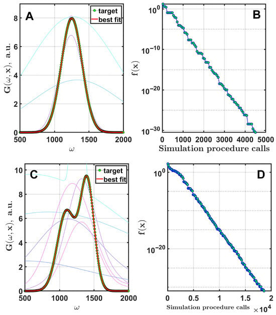
Figure 1.
Fitting of two spectrum-like curves simulated with one (A) and two (C) Gaussian functions. Thin colored lines are the current best results for the first eight generations of optimization. The overall convergence dynamics are shown in (B,D).
5.1.2. Gaussians with Almost Identical Frequencies
The next step of the research was to determine the extent to which the algorithm can distinguish between closely spaced Gaussian functions and whether there is a limit to its ability. Since the combination of two closely located Gaussians forms a function that resembles a single Gaussian, it is tempting for the optimization algorithm to try to take the easier route out and fit the combined objective function with a single Gaussian.
Based on strategy tests, the DE/rand-to-best/1/exp strategy was used with and in both cases. The number of generations was 5000, 15,000, and 30,000. Calculations were performed with six free parameters, i.e., two Gaussian functions with three parameters each (Figure 2). The intensities of the Gaussians were . Cases where the algorithm clearly identified two Gaussians were marked as “+”, and those where it failed were marked “−”. A case with two Gaussians with , and using 30,000 generations is presented in Figure 2B,C. A similar case with 150,000 generations is shown in Figure 2D.
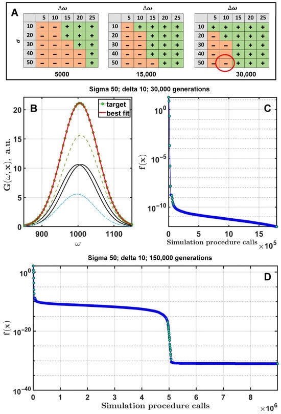
Figure 2.
Fitting of curves consisting of two Gaussians with similar frequencies. The tables on plot (A) show the distribution of successful DE runs as a function of the number of generations. The red circle indicates the case where DE failed to find the correct solution after 30,000 generations for 2 Gaussian functions with and . The green line with markers is the target function (B), which is the sum of the two black Gaussians. The green and blue dotted lines represent the resulting components after fitting. Plots (C,D) show the dynamics of the objective function at different numbers of generations.
Based on the panels of Figure 2A, it can be seen that the wider the distance between the peaks, and the narrower their width, the easier it is for the algorithm to find the specified Gaussians. As can be seen, in the vicinity of 75,000 generations (450,000 simulation procedure calls) the algorithm finds the correct solution, resulting in the target function moving towards machine epsilon (~10−32). Therefore, 150,000 generations were sufficient for the algorithm to accurately determine two closely located Gaussians. At some point, the cost function starts to converge rapidly towards machine epsilon.
5.1.3. Test with a Set of Gaussian Curves
Let us now evaluate whether EGD can achieve an acceptable result for a combination of multiple Gaussians. In Figure 3, the fitting results of the simulated spectra using eight equidistant identical Gaussian functions (A) and the eight different Gaussians (C) are presented. The Gaussian parameters are given in Table 1. The DE/rand/1/bin strategy was used, with and for the equal frequencies set, and and for the unequal set. The number of generations was 10,000 for both cases. The corresponding dynamics of the cost function are shown on the right.
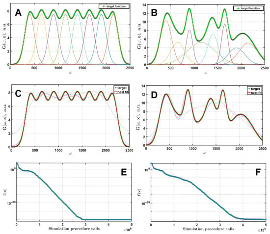
Figure 3.
Fitting of a simulated spectrum-like curve consisting of 8 identical Gaussian functions (A) and a curve consisting of 8 Gaussians with different parameters for each function (B). The results of the successful fits are presented for both cases (C,D). Thin lines indicate the current best curves immediately after beginning of the optimization. The convergence dynamics are presented in (E,F).

Table 1.
Parameters of two datasets used to generate synthetic spectral-like curves to test the EGD method.
To determine the optimal number of Gaussian functions for the synthetic spectrum, calculations were performed where the fitting was performed using different combinations of Gaussians with the number of functions varying from 4 to 12. The number of independent runs was 25, and the results for medians and means are shown in Figure 4.
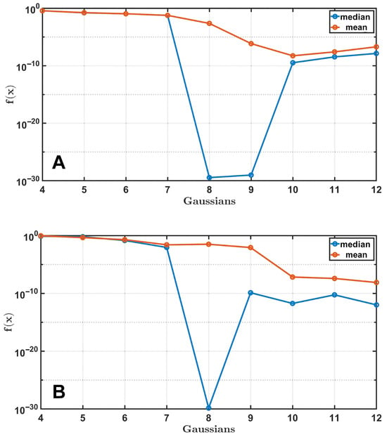
Figure 4.
A demonstration of the process of finding the optimal set of Gaussian functions. The synthetic curves shown in Figure 3 serve as target functions. The medians and means of the cost function after 100,000 generations, averaged over 25 independent DE runs, are shown for test curve 1 (A) and 2 (B).
The results show that with a smaller number of Gaussians, there will be no complete overlap between the curves. However, with a larger number, the algorithm will find a better solution, although it will be significantly slower due to the increased number of parameters in the system. This is because it takes longer to solve the optimization problem due to overdetermination. Therefore, if each Gaussian function contributes significantly and can be distinguished from the others, the DE algorithm will still be able to find this solution using the same set of parameters.
5.2. Experimental Data Fitting
In order to extend the applicability of the EGD algorithm for fitting experimental data, simulations were made for absorption spectra of chlorophyll a, bacteriochlorophyll a, spheroidene, and spheroidenone [17]. The chemical structure of the studied pigments and their absorption spectra are presented in Figure 5. An additional challenge of such modeling is the unknown optimal number of Gaussians, which requires the development of a certain criterion for the fitting procedure. Taking into account the results of the preliminary simulations, the process for determining the optimal number of Gaussians for the experimental data can be algorithmized as follows.
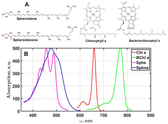
Figure 5.
The chemical structure of biological pigments (A) and their absorption spectra (B).
Evolutionary Gaussian Decomposition Algorithm
This algorithm is implemented in the following way (Algorithm 1). Before simulation starts, a guess number for the optimal number of Gaussians, , is chosen. It can take any value, but it is better to choose a reasonable number that roughly corresponds to the shape of the modeled curve. Then the search range of integer numbers is set, where δ is the width of the range; here, appeared to be good enough for the test spectra. Then DE runs 25 times for each and the mean, median, and minimum values of the objective function are saved. When the cycle is finished, one of the three possible options occurs: (i) the optimum is within the given range; the optimal number of Gaussians in decomposition is determined according to the developed criterium and optimization stops; (ii) the minimum value is on the left of (i.e., at ), becomes , and the optimization runs once again with the new search range; and (iii) the minimum value is on the right of , becomes , and the optimization runs once again, as in (ii). The program runs until it reaches (i).
| Algorithm 1. Pseudocode for the evolutionary Gaussian decomposition |
| 1: Input: the objective function and the guess number of Gaussians |
| 2: Create the boundaries ) |
| 3: if then |
| 4: , |
| 5: , |
| 6: else |
| 7: |
| 8: |
| 9: end if |
| 10: Fitting a curve with a different number of Gaussians from |
| 11: do_next_statistics = true |
| 12: while do_next_statistics do |
| 13: for |
| 14: Creating statistic for a model with the current number of Gaussians |
| 15: for to 25 |
| 16: DE: initialization |
| 17: DE: main loop |
| 18: Save |
| 19: end for |
| 20: Save the mean value |
| 21: Save the median |
| 22: Save the minimum |
| 23: Save statistic of local minima |
| 24: end for |
| 25: Analyze |
| 26: if ) then |
| 27: , |
| 28: , |
| 29: else |
| 30: if ) then |
| 31: , |
| 32: , |
| 33: else |
| 34: if (Check statistic of the local minima : if there is such that |
| 35: for there are the same and all values of |
| 36: are different) then |
| 37: do_next_statistics = false |
| 38: else |
| 39: Vary slightly parameters of DE (F,Cr) and do another while code |
| 40: do_next_statistics = true |
| 41: end if |
| 42: end if |
| 43: end if |
| 44: end while |
| 45: Output: |
The results of the fitting are presented in Figure 6. The DE/rand-to-best/1/exp strategy was used with and for all calculations with 50,000 generations. Calculations were made for the number of Gaussians , and the number of independent runs was 25. Means , medians , and minima are shown in Figure 6, and corresponding cost function values are presented in Table 2 and Table 3. The results indicate that the optimal number of Gaussian functions lies between 8 and 10. In contrast to the synthetic spectra, the minimum required number of Gaussians is not known beforehand and depends on the quality of the experimental data (signal-to-noise ratio).
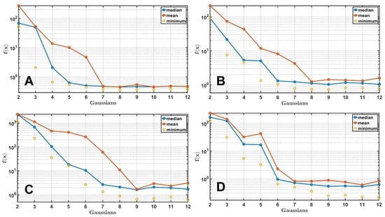
Figure 6.
Fitting the absorption spectra of Chl a (A), BChl a (B), spheroidene (C) and spheroidenone (D) in solvents. The medians, means, and minimum values of the cost function for each Gaussian combination after 25 independent DE runs are presented.

Table 2.
The statistics of for different M values while fitting the chlorophyll a and bacteriochlorophyll a spectra.

Table 3.
The statistics of for different M values while fitting the spheroidene and spheroidenone spectra.
Upon analyzing the results, an interesting pattern emerged: with a sufficient number of Gaussian functions, all solutions were unique, while with an insufficient number, groups of similar results were formed. This relationship is illustrated in more detail in Figure 7. The results suggest that the optimal number for chlorophyll is , while for the other three pigments, the optimal number is , which corresponds to the optimal range shown in Figure 6. An example of the best fit for each pigment can be seen in Figure 8, with the corresponding dynamics of the cost function shown on the right. Despite the significant differences in the initial generations, the algorithm achieves a good agreement between the experimental and simulated spectra by the end of the process for all pigments.
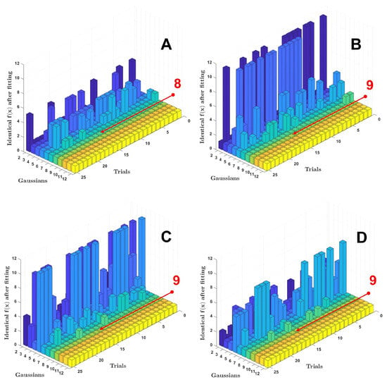
Figure 7.
3D bar graphs representing the statistics of the cost function values for the experimental data of Chl a (A), BChl a (B), spheroidene (C), and spheroidenone (D). The z-axis corresponds to the number of identical values.
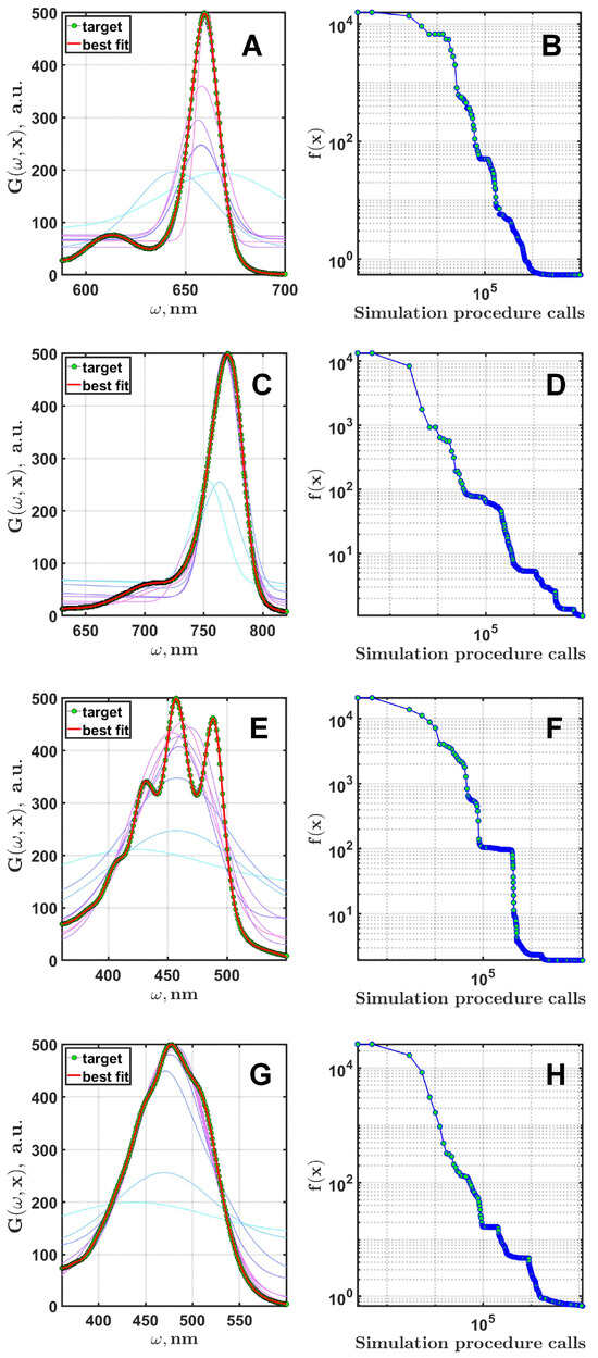
Figure 8.
The results of the fitting for Chl a (A), BChl a (C), spheroidene (E), and spheroidenone (G). The thin lines indicate the best spectra after first seven generations of the optimization process. The corresponding convergence dynamics are shown in (B,D,F,H) on logarithmic scales.
6. Discussion
6.1. Synthetic Data Fitting
In the synthetic data, a sharp decrease in the cost function can be observed when a sufficient number of Gaussian components is reached. This can be considered one of the indicators of an optimal value (Figure 4). With a number of Gaussian components less than in the synthetic spectrum (target function), the modeled spectrum cannot completely match the target one. For cases where the Gaussian functions are noticeably different from each other and their contributions to the spectrum are clearly visible, the optimal number equals the number of components in the target spectrum (Figure 3B).
When there are a large number of Gaussian components, some of them may be completely nullified or their intensities may be divided between several components, thereby fitting one Gaussian in the synthetic spectrum. If the number of Gaussian components significantly exceeds the number in the target spectrum, the situation becomes more complex. There may be a complete elimination of “extra” components or different variations in the intensity distribution, where each component will be significant.
6.2. Experimental Data Fitting
Similar calculations were made for the experimental spectra as target functions. One significant difference from previous fits is that the algorithm initially does not know how many Gaussian components are present in the spectrum, and it finds the optimal number during the modeling process.
For experimental spectra, the behavior of the cost function during the optimization differs from that of synthetic data. As the number of Gaussian components increases, the minimum constantly decreases (Figure 6). This is because the experimental data always contain a noise component, and with each additional Gaussian function, the accuracy of the fit increases. It is also worth noting that when is clearly insufficient (Figure 6, range from 2 to 6), , , and decrease fast and then reach plateaus where they fluctuate slightly within the error bounds as the number of Gaussians is further increased. is definitely located around the point when the plateau begins.
In analyzing the data, we tried to identify characteristics in the fitting process that could be used as a criterion for determining the minimum number of Gaussians needed. Parameters, such as the mean and minimum values of the object function, are used to assess the quality of the fitting. Interestingly, unlike DE, the genetic algorithm has been used more than once to optimize the decomposition of experimental optical spectra into Gaussian functions [29,37]. However, the main drawback of these studies is the use of the genetic algorithm itself and the lack of a clear criterion for determining how many Gaussian functions will be sufficient for the decomposition to be considered acceptable. In this study, an original criterion was developed based on estimating the frequency of local minima reached by the DE algorithm during optimization (see pseudocode). Figure 7 shows statistics on these local minima. When fitting experimental spectra with an insufficient number of Gaussian functions, many solutions form groups of local minima (bars in Figure 7). These groups disappear when the system is overdetermined, which can also be seen as an implicit indication of the optimal number of Gaussians. However, further study is needed to fully understand this feature. It is important to note that the disappearance of local minima often coincides with the alignment of the mean, median, and, in some cases, the minimum values of the objective function.
The decomposition of spectra into Gaussian components is widely used in research, especially in areas where the measured spectra are known to have a Gaussian line profile of a combination of Gaussians. For instance, there is a study that proposes a method for analyzing the spectra of neutral hydrogen in galaxy spectra [9]. This method combines derivative spectroscopy and a machine learning technique. Interestingly, the study compares the effectiveness of this method with traditional manual fitting of the spectra. Another method of identifying bands in spectra was proposed based on the Bayesian Monte Carlo algorithm [48], which demonstrated some success in detecting absorption lines with a low signal-to-noise ratio. Actually, Monte Carlo simulation is used in many applications to fit spectra [11,49]. It is important to note that evolutionary algorithms, such as DE, use Monte Carlo ideas at the initial stage of their evolution. However, they move on to a more sophisticated evolution of parameter modification. Evolutionary algorithms allow us to explore a large number of possibilities, especially if the computational procedures are not resource-consuming, such as Gaussian decomposition.
7. Conclusions
While investigating the convergence of the DE algorithm in solving problems related to modeling the optical response of organic pigments, we have encountered the classic issue of premature convergence, which is common for many types of optimization algorithms. Our recent research has led to the development of a specific procedure that can be applied in conjunction with the classic DE algorithm to significantly improve its performance in certain applications [44]. During this work, it became clear that even such problems as local minima can be utilized to analyze experimental data, as they provide valuable insights into the optimization process.
Thus, the idea of analyzing the frequency with which an optimization algorithm become stuck in local minima was incorporated into the proposed implementation of a widely used method known as Gaussian decomposition. By investigating the behavior of DE on both synthetic and experimental data, an evolutionary Gaussian decomposition (EGD) method was developed that allows us to estimate the minimum number of Gaussians required for the decomposition. This number represents the limit beyond which the quality of the fit for the studied spectrum or function does not significantly improve.
The main feature of EGD is its analysis of the statistics of reaching local minima (see Figure 7). EGD calculates the number of times optimization completes with the same objective function values. By comparing the mean, median, and minimum values of the objective function, we conclude that analyzing the statistic of local minima can be useful for determining the optimal number of Gaussians in a decomposition.
Author Contributions
Supervision, conceptualization, software, and writing—review and editing, R.Y.P.; writing—review and editing, software, and investigation, D.D.C.; software and investigation, V.A.K.; validation, formal analysis, visualization, and investigation, A.P.R.; conceptualization and methodology, S.V.G.; conceptualization, methodology, and visualization, A.S.D.; supervision, methodology, and funding acquisition, A.Y.I. All authors have read and agreed to the published version of the manuscript.
Funding
This research was funded by a grant from the Ministry of Science and Higher Education of the Russian Federation, grant number 075-15-2024-540.
Institutional Review Board Statement
Not applicable.
Informed Consent Statement
Not applicable.
Data Availability Statement
No additional data available.
Conflicts of Interest
The authors declare no conflict of interests. The funders had no role in the design of the study; in the collection, analyses, or interpretation of data; in the writing of the manuscript; or in the decision to publish the results.
Abbreviations
The following abbreviations are used in this manuscript:
| DE | Differential evolution |
| GD | Gaussian decomposition |
| EGD | Evolutionary Gaussian decomposition |
References
- Nikita, S.; Bhattacharya, S.; Manocha, K.; Rathore, A.S. Deep learning framework for peak detection at the intact level of therapeutic proteins. J. Sep. Sci. 2024, 47, e2400051. [Google Scholar] [CrossRef]
- Döring, A.; Qiu, Y.; Rogach, A.L. Improving the accuracy of carbon dot temperature sensing using multi-dimensional machine learning. ACS Appl. Nano Mater. 2024, 7, 2258–2269. [Google Scholar] [CrossRef]
- Mukamel, S. Principles of Nonlinear Optical Spectroscopy; Oxford University Press: New York, NY, USA; Oxford, UK,, 1995; Volume 6, p. 543. [Google Scholar]
- Massicotte, P.; Markager, S. Using a gaussian decomposition approach to model absorption spectra of chromophoric dissolved organic matter. Mar. Chem. 2016, 180, 24–32. [Google Scholar] [CrossRef]
- Kramynin, S.P. On the possibility of decomposition of integral spectra represented by a superposition of gaussian, lorentz and pseudo-voigt profiles. Solid State Commun. 2025, 397, 115806. [Google Scholar] [CrossRef]
- Liu, J.; Zhang, X.; Lv, J.; Li, X.; Du, L. Gaussian decomposition method for full waveform data of lidar base on neural network. Sci. Rep. 2025, 15, 5639. [Google Scholar] [CrossRef]
- Stutzki, J.; Güsten, R. High spatial resolution isotopic co and cs observations of m17 sw: The clumpy structure of the molecular cloud core. Astrophys. J. 1990, 356, 513–533. [Google Scholar] [CrossRef]
- Haud, U. Gaussian decomposition of the leiden/dwingeloo survey—I. Decomposition algorithm. Astron. Astrophys. 2000, 364, 83–101. [Google Scholar]
- Lindner, R.R.; Vera-Ciro, C.; Murray, C.E.; Stanimirović, S.; Babler, B.; Heiles, C.; Hennebelle, P.; Goss, W.M.; Dickey, J. Autonomous gaussian decomposition. Astron. J. 2015, 149, 138. [Google Scholar] [CrossRef]
- Petzler, A.; Dawson, J.R.; Wardle, M. Amoeba: Automated molecular excitation bayesian line-fitting algorithm. Astrophys. J. 2021, 923, 261. [Google Scholar] [CrossRef]
- Juvela, M.; Tharakkal, D. Fast fitting of spectral lines with gaussian and hyperfine structure models. Astron. Astrophys. 2024, 685, A164. [Google Scholar] [CrossRef]
- Fernández-González, A.; Montejo-Bernardo, J.M. Natural logarithm derivative method: A novel and easy methodology for finding maximums in overlapping experimental peaks. Spectrochim. Acta Part A Mol. Biomol. Spectrosc. 2009, 74, 714–718. [Google Scholar] [CrossRef]
- Wang, Q.; Chen, H.; Hu, S.; Zhao, Y.; Chen, H. Curve-fitting analysis of micro ft-ir and its application on individual oil inclusion and micro-area bitumens. Earth Sci. China Univ. Geosci. 2016, 41, 1921–1934. [Google Scholar] [CrossRef]
- Pavlov, E. Applying hierarchical mappings to describe gaussian spectrum of luminescence. Eur. Phys. J. Plus 2022, 137, 1–5. [Google Scholar] [CrossRef]
- Li, K.; Zhang, Y.; Li, Y. A false peak recognition method based on deep learning. Chemometr. Intell. Lab. Syst. 2023, 238, 104849. [Google Scholar] [CrossRef]
- Dubrovkin, J. Evaluation of undetectable perturbations of peak parameters estimated by the least square curve fitting of analytical signal consisting of overlapping peaks. Chemometr. Intell. Lab. Syst. 2016, 153, 9–21. [Google Scholar] [CrossRef]
- Razjivin, A.P.; Kozlovsky, V.S.; Ashikhmin, A.A.; Pishchalnikov, R.Y. Gaussian decomposition vs. Semiclassical quantum simulation: Obtaining the high-order derivatives of a spectrum in the case of photosynthetic pigment optical properties studying. Sensors 2023, 23, 8248. [Google Scholar] [CrossRef]
- Kovalenko, A.V.; Vovk, S.M.; Plakhtii, Y.G. Sum decomposition method for gaussian functions comprising an experimental photoluminescence spectrum. J. Appl. Spectrosc. 2021, 88, 357–362. [Google Scholar] [CrossRef]
- Kramynin, S.P.; Zobov, E.M.; Zobov, M.E. Decomposition of aiibvi semiconductor compounds integral photoluminescence spectra using mathematical and computer analysis. J. Lumin. 2022, 252, 119432. [Google Scholar] [CrossRef]
- Zhang, J.; Gonzalez, E.; Hestilow, T.; Haskins, W.; Huang, Y. Review of peak detection algorithms in liquid-chromatography-mass spectrometry. Curr. Genom. 2009, 10, 388–401. [Google Scholar] [CrossRef]
- Schulze, H.G.; Atkins, C.G.; Devine, D.V.; Blades, M.W.; Turner, R.F.B. Fully automated decomposition of raman spectra into individual pearson’s type vii distributions applied to biological and biomedical samples. Appl. Spectrosc. 2015, 69, 26–36. [Google Scholar] [CrossRef]
- Kumanan, T.S.; Sofi, A. Waste-based evolution of elasticity in altered lime adobe units with explanatory predictions of peak functions models. Innov. Infrastruct. Solut. 2024, 9, 337. [Google Scholar] [CrossRef]
- Nguyen, A.Q.D.; Nguyen, V.H.; Lee, H.Y. Gaussian decomposition method in designing a freeform lens for an led fishing/working lamp. Curr. Opt. Photonics 2017, 1, 233–238. [Google Scholar] [CrossRef]
- De Weljer, A.P.; Lucaslus, C.B.; Buydens, L.; Kateman, G.; Heuvel, H.M.; Mannee, H. Curve fitting using natural computation. Anal. Chem. 1994, 66, 23–31. [Google Scholar] [CrossRef]
- Karakaplan, M. Fitting lorentzian peaks with evolutionary genetic algorithm based on stochastic search procedure. Anal. Chim. Acta 2007, 587, 235–239. [Google Scholar] [CrossRef]
- Zhang, B.; Yu, H.; Sun, L.; Xin, Y.; Conga, Z. A method for resolving overlapped peaks in laser-induced breakdown spectroscopy (libs). Appl Spectrosc 2013, 67, 1087–1097. [Google Scholar] [CrossRef]
- Rosas-Román, I.; Meneses-Nava, M.A.; Barbosa-García, O.; Maldonado, J.L. Simultaneous height adjust fitting: An alternative automated fitting procedure for laser-induced plasma spectra composed by multiple lorentzian profiles. Spectrochim. Acta Part B At. Spectrosc. 2017, 134, 1–5. [Google Scholar] [CrossRef]
- Meneses-Nava, M.A. Automatic spectral fitting for libs and raman spectra by boosted deconvolution method. Chemometr. Intell. Lab. Syst. 2025, 258, 105334. [Google Scholar] [CrossRef]
- Karakaplan, M.; Avcu, F.M. A parallel and non-parallel genetic algorithm for deconvolution of nmr spectra peaks. Chemometr. Intell. Lab. Syst. 2013, 125, 147–152. [Google Scholar] [CrossRef]
- Gwizdałła, T.M.; Moneta, M.E. Mössbauer distribution fitting by using global optimization approach. Nucl. Instrum. Methods Phys. Res. Sect. B Beam Interact. Mater. At. 2012, 279, 205–207. [Google Scholar] [CrossRef]
- Telikani, A.; Tahmassebi, A.; Banzhaf, W.; Gandomi, A.H. Evolutionary machine learning: A survey. ACM Comput. Surv. 2021, 54, 1–35. [Google Scholar] [CrossRef]
- Ahmad, M.F.; Isa, N.A.M.; Lim, W.H.; Ang, K.M. Differential evolution: A recent review based on state-of-the-art works. Alex. Eng. J. 2022, 61, 3831–3872. [Google Scholar] [CrossRef]
- Katoch, S.; Chauhan, S.S.; Kumar, V. A review on genetic algorithm: Past, present, and future. Multimed. Tools Appl. 2021, 80, 8091–8126. [Google Scholar] [CrossRef]
- Haupt, R.L.; Haupt, S.E. Practical Genetic Algorithms; Wiley-Blackwell: Hoboken, NJ, USA, 2004; pp. 1–253. [Google Scholar] [CrossRef]
- Gudkov, S.V.; Sarimov, R.M.; Astashev, M.E.; Pishchalnikov, R.Y.; Yanykin, D.V.; Simakin, A.V.; Shkirin, A.V.; Serov, D.A.; Konchekov, E.M.; Gusein-Zade, N.G.; et al. Modern physical methods and technologies in agriculture. Phys.-Uspekhi 2024, 67, 194–210. [Google Scholar] [CrossRef]
- Leardi, R. 1.24—Genetic algorithms in chemistry. In Comprehensive Chemometrics: Chemical and Biochemical Data Analysis, 2nd ed.; Elsevier: Amsterdam, The Netherlands, 2020; Volume 1, pp. 617–634. [Google Scholar] [CrossRef]
- Avcu, F.M.; Karakaplan, M. Finding exact number of peaks in broadband uv-vis spectra using curve fitting method based on evolutionary computing. J. Turk. Chem. Soc. Sec. A Chem. 2020, 7, 117–124. [Google Scholar] [CrossRef]
- Karakaplan, M.; Avcu, F.M. Deconvolution of gaussian peaks with mixed real and discrete-integer optimization based on evolutionary computing. J. Chemometr. 2020, 34, e3229. [Google Scholar] [CrossRef]
- Zhu, Q.; Gao, K.; Liu, Y. Meta-heuristics for solving curve fitting problems in optical-diffraction based image depth reconstruction. In Proceedings of the 3rd IEEE International Conference on Software Engineering and Artificial Intelligence (SEAI 2023), Xiamen, China, 16–18 June 2023; Institute of Electrical and Electronics Engineers Inc.: New York, NY, USA, 2023; pp. 178–183. [Google Scholar] [CrossRef]
- Polo-Corpa, M.J.; Salcedo-Sanz, S.; Pérez-Bellido, A.M.; López-Espí, P.; Benavente, R.; Pérez, E. Curve fitting using heuristics and bio-inspired optimization algorithms for experimental data processing in chemistry. Chemometr. Intell. Lab. Syst. 2009, 96, 34–42. [Google Scholar] [CrossRef]
- Alfar, I.J.; Khorshidtalab, A.; Akmeliawati, R.; Ahmad, S.; Jaswir, I. Towards authentication of beef, chicken and lard using micro near-infrared spectrometer based on support vector machine classification. ARPN J. Eng. Appl. Sci. 2016, 11, 4130–4136. [Google Scholar]
- Storn, R. System design by constraint adaptation and differential evolution. IEEE Trans. Evol. Comput. 1999, 3, 22–34. [Google Scholar] [CrossRef]
- Storn, R.; Price, K. Differential evolution—A simple and efficient heuristic for global optimization over continuous spaces. J. Glob. Optim. 1997, 11, 341–359. [Google Scholar] [CrossRef]
- Chesalin, D.D.; Pishchalnikov, R.Y. A local minima escape procedure to improve the convergence of differential evolution. Appl. Soft Comput. 2025, 171, 112753. [Google Scholar] [CrossRef]
- Bilal; Pant, M.; Zaheer, H.; Garcia-Hernandez, L.; Abraham, A. Differential evolution: A review of more than two decades of research. Eng. Appl. Artif. Intell. 2020, 90, 103479. [Google Scholar] [CrossRef]
- Chesalin, D.D.; Kulikov, E.A.; Yaroshevich, I.A.; Maksimov, E.G.; Selishcheva, A.A.; Pishchalnikov, R.Y. Differential evolution reveals the effect of polar and nonpolar solvents on carotenoids: A case study of astaxanthin optical response modeling. Swarm Evol. Comput. 2022, 75, 101210. [Google Scholar] [CrossRef]
- Lawton, W.H.; Sylvestre, E.A. Self modeling curve resolution. Technometrics 1971, 13, 617–633. [Google Scholar] [CrossRef]
- Allison, J.R.; Sadler, E.M.; Whiting, M.T. Application of a bayesian method to absorption spectral-line finding in simulated askap data. Publ. Astron. Soc. Aust. 2013, 29, 221–228. [Google Scholar] [CrossRef]
- Feroz, F.; Hobson, M.P.; Bridges, M. Multinest: An efficient and robust bayesian inference tool for cosmology and particle physics. Mon. Not. R. Astron. Soc. 2009, 398, 1601–1614. [Google Scholar] [CrossRef]
Disclaimer/Publisher’s Note: The statements, opinions and data contained in all publications are solely those of the individual author(s) and contributor(s) and not of MDPI and/or the editor(s). MDPI and/or the editor(s) disclaim responsibility for any injury to people or property resulting from any ideas, methods, instructions or products referred to in the content. |
© 2025 by the authors. Licensee MDPI, Basel, Switzerland. This article is an open access article distributed under the terms and conditions of the Creative Commons Attribution (CC BY) license (https://creativecommons.org/licenses/by/4.0/).