Article

Temperature-Compensated Multi-Objective Framework for Core Loss Prediction and Optimization: Integrating Data-Driven Modeling and Evolutionary Strategies

State Key Laboratory of Deep Earth Exploration and Imaging, School of Engineering and Technology, China University of Geosciences (Beijing), Beijing 100083, China
*
Author to whom correspondence should be addressed.
Mathematics 2025, 13(17), 2758; https://doi.org/10.3390/math13172758
Submission received: 16 July 2025 / Revised: 25 August 2025 / Accepted: 25 August 2025 / Published: 27 August 2025
(This article belongs to the Special Issue Multi-Objective Optimization and Applications)

Abstract

Magnetic components serve as critical energy conversion elements in power conversion systems, with their performance directly determining overall system efficiency and long-term operational reliability. The development of accurate core loss frameworks and multi-objective optimization strategies has emerged as a pivotal technical bottleneck in power electronics research. This study develops an integrated framework combining physics-informed modeling and multi-objective optimization. Key findings include the following: (1) a square-root temperature correction model (exponent = 0.5) derived via nonlinear least squares outperforms six alternatives for Steinmetz equation enhancement; (2) a hybrid Bi-LSTM-Bayes-ISE model achieves industry-leading predictive accuracy (R2 = 96.22%) through Bayesian hyperparameter optimization; and (3) coupled with NSGA-II, the framework optimizes core loss minimization and magnetic energy transmission, yielding Pareto-optimal solutions. Eight decision-making strategies are compared to refine trade-offs, while a crow search algorithm (CSA) improves NSGA-II’s initial population diversity. UFM, as the optimal decision strategy, achieves minimal core loss (659,555 W/m3) and maximal energy transmission (41,201.9 T·Hz) under 90 °C, 489.7 kHz, and 0.0841 T conditions. Experimental results validate the approach’s superiority in balancing performance and multi-objective efficiency under thermal variations.

1. Introduction

Amidst the rapid progression of power electronics toward higher frequencies and power densities, magnetic components serve as critical energy conversion elements in power conversion systems, with their performance directly determining overall system efficiency and long-term operational reliability [1,2,3]. The proliferation of wide-bandgap semiconductor devices has pushed switching frequencies into the MHz regime [4], imposing significant challenges in thermal management [5], electromagnetic interference (EMI) mitigation [6,7,8], and efficiency optimization [9,10]. Against this backdrop, the development of accurate core loss modeling frameworks and multi-objective optimization strategies has emerged as a pivotal technical bottleneck in power electronics research.
Power losses in magnetic components comprise two primary components: winding losses and core losses [11,12,13]. Winding losses, originating from Joule heating in conductive materials, can be quantitatively assessed through finite element analysis (FEA) incorporating high-frequency skin effect corrections [14,15]. In contrast, core loss mechanisms exhibit greater complexity, arising from irreversible energy dissipation caused by magnetic domain wall motion, eddy currents, and residual losses under alternating magnetic fields [16,17,18]. According to Bertotti’s seminal theory, total core loss can be decomposed into three distinct contributions: hysteresis loss (linearly proportional to magnetization frequency), eddy current loss (quadratic dependency on frequency), and residual loss (encompassing relaxation phenomena and other complex mechanisms) [13,19,20]. This intrinsic nonlinearity positions core loss as a critical limiting factor for system energy efficiency: (1) Joule heating from losses accelerates material degradation and induces thermal runaway risks [21]. (2) Nonlinear loss characteristics may deteriorate EMI spectral distributions, compromising electromagnetic compatibility (EMC) [6]. Consequently, the establishment of high-precision core loss prediction models holds strategic importance for achieving the tripartite objectives of “high efficiency—high density—high reliability”.
The existing representative core loss analysis methods in recent years are shown in Table 1. The physical mechanisms governing core losses involve profound coupling between material microstructures and macroscopic electromagnetic parameters [22,23]. Empirical studies reveal that loss characteristics depend not only on intrinsic material properties such as permeability and coercivity but also exhibit complex nonlinear relationships with operational parameters including frequency [24], flux density amplitude [25], ambient temperature [26,27,28], and excitation waveforms [29,30]. While classical models like the Steinmetz Equation provide a theoretical foundation for loss calculation, their assumptions of sinusoidal excitation and isothermal conditions limit practical applicability, particularly under non-sinusoidal or thermally varying conditions [31,32]. Recent data-driven approaches demonstrate superior adaptability. Oumiguil and Nejmi [33] employed extreme gradient boosting (XGBoost) to daily PV power forecasting, while Liu and Liang [34] implemented a CNN-Bi-LSTM architecture for small-sample loss prediction. Yu et al. [35] explored the energy loss and heat generated by high-speed solenoid valves (HSV) under high-frequency operating conditions and utilized NSGA-II to provide efficient HSV driving strategy optimization. Shen et al. [36] combined the enhancement method of GAN with NSGA-II to calculate the multi-objective optimization of core loss. Core loss prediction and optimization is an issue that is receiving increasing attention [30,37,38].
However, there are still the following three challenges at present: (1) The traditional core loss model (Stanmetz equation) has relatively limited applicability, as it is primarily derived for sinusoidal excitations and temperature-invariant scenarios, resulting in significant errors in practical engineering applications when applied to non-sinusoidal waveforms or thermally dynamic conditions. (2) Traditional empirical models are limited in accuracy when dealing with complex waveforms (such as other triangular and trapezoidal waves), nonlinear temperature rise effects (abnormal changes in core losses at different temperatures), and the coupling effects of multiple factors (magnetic energy, temperature, waveforms, etc.). These limitations necessitate data-driven deep learning approaches to enhance predictive capability. (3) In engineering applications, the design of magnetic cores should not only focus on minimizing losses but also take into account the efficiency of magnetic energy transmission simultaneously to ensure multi-objective optimization.
This study proposes a multi-dimensional core loss analysis framework. First, a temperature-compensated Steinmetz Equation is developed by introducing six nonlinear correction strategies (linear, exponential, logarithmic, quadratic, square root, and multiplicative models), with comparative analysis of prediction accuracy under variable thermal conditions. Second, a Bayesian-optimized BiLSTM (BiLSTM-Bayes) deep learning model is constructed to capture temporal dependencies in excitation waveforms, demonstrating superior performance in modeling nonlinear loss behaviors. Finally, a multi-objective optimization paradigm is established combining the following: (1) a BiLSTM-Bayes-ISE core loss predictor as the objective function; and (2) magnetic energy transfer efficiency as an additional optimization target. The NSGA-II is employed to generate Pareto front, with crow search algorithm (CSA)-enhanced initial population initialization improving convergence characteristics. Through comparative analysis of eight decision-making strategies (weighted sum, utility function, etc.), optimal operational conditions achieving simultaneous core loss minimization and transmitted magnetic energy maximization are identified.

2. Methodology

2.1. Classical Core Loss Equation (SE) and Improved Strategy (ISE)

2.1.1. Classical Core Loss Equation (SE)

The Steinmetz Equation (SE), as a classic core loss prediction model, is widely applied in fields such as power electronic transformers and magnetic components [39]. SE is expressed as follows:
P = k f α B m β
where P is the core loss; Bm is the peak (maximum) of magnetic flux density; f is the frequency; and k, α, and β are the coefficients related to the material properties fitted from experimental data. The effect evaluation of coefficient fitting adopts the following five indicators.
(1)
Max Error
Max Error reflects the prediction error of the model in the worst case. The smaller the Max Error, the better the prediction of the model.
M a x E r r o r = max T r u e P r e
(2)
Mean squared error (MSE)
MSE is the average of the squared errors and is highly sensitive to large errors and outliers. The smaller the MSE, the closer the predicted value is to the true value.
M S E = 1 n i = 1 n T r u e P r e 2
(3)
Root mean squared error (RMSE)
RMSE is the square root of the mean squared error and can visually reflect the prediction error. The smaller the RMSE, the higher the prediction accuracy of the model.
R M S E = 1 n i = 1 n T r u e P r e 2
(4)
Mean Absolute Error (MAE)
MAE is the average value of the absolute values of errors, reflecting the average degree of error. The smaller the MAE, the smaller the average prediction error of the model.
M A E = 1 n i = 1 n T r u e P r e
(5)
Coefficient of determination (R2)
R2 reflects the degree of fit between the predicted value and the true value, with a value range of [0, 1]. The closer R2 is to 1, the higher the accuracy of the model.
R 2 = 1 i = 1 n T r u e P r e 2 i = 1 n T r u e A v e 2

2.1.2. Improved Core Loss Equation (ISE)

Recognizing the limitations of the classical Steinmetz Equation (SE) under non-sinusoidal excitations and thermally varying conditions, this study proposes a systematic temperature-compensated modeling approach. The original SE exhibits significant prediction errors under temperature deviations from the reference condition (T0 = 25 °C). To address this, six temperature correction strategies were formulated by introducing a thermal modification factor Φ(T) into the original SE framework as follows:
P = k f α B m β Φ T
We selected six different improved equations, hoping to compare their accuracy to determine the final improvement method. The functions were chosen to represent plausible temperature-loss relationships observed in magnetic materials (e.g., linear thermal expansion at low temperatures, nonlinear saturation effects at elevated temperatures). The set includes linear, exponential, logarithmic, polynomial, radical, and multiplicative forms to comprehensively capture potential thermal dependencies. All functions contain a minimal number of parameters (k, α, β, C) to avoid overfitting while retaining sufficient flexibility for curve fitting. Mathematical formulations are detailed below.
(1)
Linear Correction:
Φ T = 1 + C ( T T 0 )
(2)
Exponential Correction:
Φ T = e C T T 0
(3)
Logarithmic Correction:
Φ T = 1 + C log ( 1 + T T 0 )
(4)
Quadratic Correction:
Φ T = 1 + C ( T T 0 ) 2
(5)
Square Root Correction:
Φ T = 1 + C T T 0
(6)
Multiplicative Correction:
Φ T = 1 + T T 0 C
where T is the current working temperature, and T0 is the normal laboratory temperature (25 °C); k, α, β and C are the coefficients related to the material properties fitted from experimental data.

2.2. Core Loss Prediction Model Based on Bi-LSTM-Bayes-ISE

2.2.1. Bi-LSTM Method

The accuracy of traditional empirical models is limited when dealing with complex waveforms, nonlinear temperature rise effects, and the coupling of multiple factors. Therefore, it is necessary to rely on data-driven deep learning methods to enhance the predictive ability. To select the optimal model, we conducted a comparative study of three machine learning models (SVR, Decision Tree, Linear Regression) and two deep learning models (LSTM and GRU). To this end, this study proposes a core loss prediction framework based on Bi-LSTM (Figure 1). Results showed that Bi-LSTM outperformed other models in capturing bidirectional contextual information (forward/backward waveform history) and handling multi-factor interactions. This model can effectively capture the nonlinear influence of historical information of the excitation waveform on the current loss.

2.2.2. Bayesian Optimization Algorithm

Bayesian Optimization employs Gaussian Processes to iteratively refine prior distributions by observing objective function outputs at sampled input points [40]. This method demonstrates superior computational efficiency, achieving rapid convergence with significantly fewer iterations compared to traditional approaches. As illustrated in Figure 2, the framework jointly optimizes multiple hyperparameters in a model-driven paradigm, capturing synergistic interactions through advanced acquisition strategies. By integrating techniques such as Tree-structured Parzen Estimator (TPE), Adaptive TPE (ATPE), and Gaussian Process (GP), the algorithm systematically identifies optimal hyperparameters for core loss prediction tasks.

2.2.3. Bi-LSTM-Bayes-ISE Framework

The Bi-LSTM-Bayes-ISE framework constitutes an integrated predictive methodology for core loss estimation. The workflow commences with data preprocessing encompassing temperature, excitation waveform, material type, and core loss measurements, followed by feature encoding of categorical variables while designating specific core loss per unit volume as the target variable. A data-driven predictive model is initially developed using Bi-LSTM. Subsequently, Bayesian hyperparameter optimization is employed to globally tune critical architectural parameters including network depth, hidden neuron count, and learning rate, resulting in the Bi-LSTM-Bayes configuration. Building upon this, the framework integrates a physics-informed Steinmetz Equation (SE) correction module to refine predictions through domain-specific knowledge, culminating in the final Bi-LSTM-Bayes-ISE model. Quantitative evaluation through comparative analysis of prediction errors before and after optimization demonstrates the framework’s capacity to systematically enhance accuracy while maintaining computational efficiency.

2.3. Core Loss Optimization Model Based on NSGA-II-CSA

2.3.1. NSGA-II

Multi-objective optimization problems (MOOs) are prevalent in engineering design, characterized by conflicting objective functions that preclude resolution through conventional single-objective optimization methods [41]. The NSGA-II represents a classical and computationally efficient evolutionary algorithm framework, widely implemented in complex engineering optimization domains including power electronics, electric machine design, structural optimization, and path planning [42].
Formally, the MOO formulation seeks decision variables xχ that simultaneously optimize multiple objective functions fi(x) under the constraint that no solution pair exhibits mutual dominance. The set of objective functions for NSGA-II is defined as follows:
min F x = f 1 x , f 2 x , , f m x T , x χ
Define two solutions x1 and x2 that satisfy the following conditions:
i , f i x 1 f i x 2 j , f j x 1 f j x 2
Then it is said that x1 governs x2. In engineering applications, the design of magnetic cores should not only focus on minimizing losses but also take into account the efficiency of magnetic energy transmission simultaneously. Therefore, in this paper, a multi-objective optimization model is further constructed based on the Bi-LSTM-Bayes-ISE prediction model to simultaneously optimize the two major objectives of core loss and magnetic energy transmission.

2.3.2. Crow Search Algorithm (CSA)

The CSA is employed to dynamically calibrate NSGA-II’s operational parameters as pragmatic tools for specific applications (addressing hyperparameter-induced variability in multi-objective electromagnetic optimization) [43,44,45]. Rooted in a probabilistic model of crows’ caching behavior, CSA introduces stochastic perturbation mechanisms to balance exploration and exploitation [46]. In this framework, CSA adapts NSGA-II’s population size, crossover probability, and mutation rate based on solution diversity metrics and convergence progress. The algorithm initializes a population of candidate parameter sets, iteratively refining them through the following: (1) global search via Levy flight-inspired jumps to escape local optima, and (2) local refinement through neighborhood-based adjustments. Empirical validation on benchmark functions demonstrates CSA’s capacity to maintain stable convergence trajectories while preserving Pareto front diversity [47,48]. This integration specifically targets the non-convex optimization landscape of core loss minimization, where traditional parameter tuning often struggles to balance computational efficiency and solution quality [45,49].

2.3.3. Pareto Front and Solution Strategies

NSGA-II finds the Pareto Optimal Set, which together constitute the optimal frontier curve or surface in the target space [49,50]. The Pareto solution set is a group of non-dominated solutions in multi-objective optimization, meaning that these solutions cannot improve another objective without sacrificing the performance of one. In fact, choosing an optimal solution (or the most representative one) from the relevant Pareto solution set requires the adoption of certain decision-making methods.
It may not be possible to find a global optimum by only one method. Eight different decision-making methods were adopted to obtain the optimal solution, namely, the Weigiht Sum Method (WSM), Ideal Point Method (IPM), Entropy Weight Method (EWM), Technique for Order Preference by Similarity to an Ideal Solution (TOPSIS) Method, Utility Function Method (UFM), Ranking-Based Selection Method (RBSM), Interactive Method (IM), and Hierarchical Optimization Method (HOM). The selection of eight decision-making methods was driven by the need to comprehensively evaluate trade-offs between core loss minimization and magnetic energy transmission efficiency under diverse operational scenarios. These methods were chosen to represent distinct decision-making philosophies. This selection strategy ensures robustness against method-specific limitations while covering all major multi-criteria decision-making (MCDM) paradigms. By incorporating this diversity, we ensure robustness against method-specific biases while capturing variations in engineering priorities (e.g., cost-sensitive vs. performance-critical applications).
(1)
Weight Sum Method (WSM)
J = i = 1 n w i f i x
where wi is normalized weights satisfying Σwi = 1, and fi is objective function.
(2)
Ideal Point Method (IPM)
d j = i 1 n f i x j f i * f i * f i n a d 2
where fi* is the ideal value, finad is the nadir value, and xj is Pareto solution.
(3)
Entropy Weight Method (EWM)
e i = k j = 1 m p i j ln p i j , k > 0
p i j = f i j j = 1 m f i j
where fij is the normalized objective value.
(4)
TOPSIS Method
C i = d i d i + d i +
where di+ and di- are the distance to idea and anti-ideal solutions, respectively.
(5)
Utility Function Method (UFM)
U x = i = 1 n ϕ i f i x , ϕ i 0
where ϕ i is the monotonic utility function reflecting decision-maker preferences.
(6)
Ranking-Based Selection Method (RBSM)
R j = i = 1 n 1 r i j
where rij is the rank of solution j for objective i (1 = best).
(7)
Interactive Method (IM)
x k + 1 = arg min x P F i = 1 n λ i k f i x
where λi(k) are the preference weights updated in iteration k.
(8)
Hierarchical Optimization Method (HOM)
min x P F f 1 x s . t . f 2 x ε 2 , , f n x ε n
where εi are the predefined thresholds for lower-priority objectives.

2.4. The Proposed Prediction and Optimization Framework

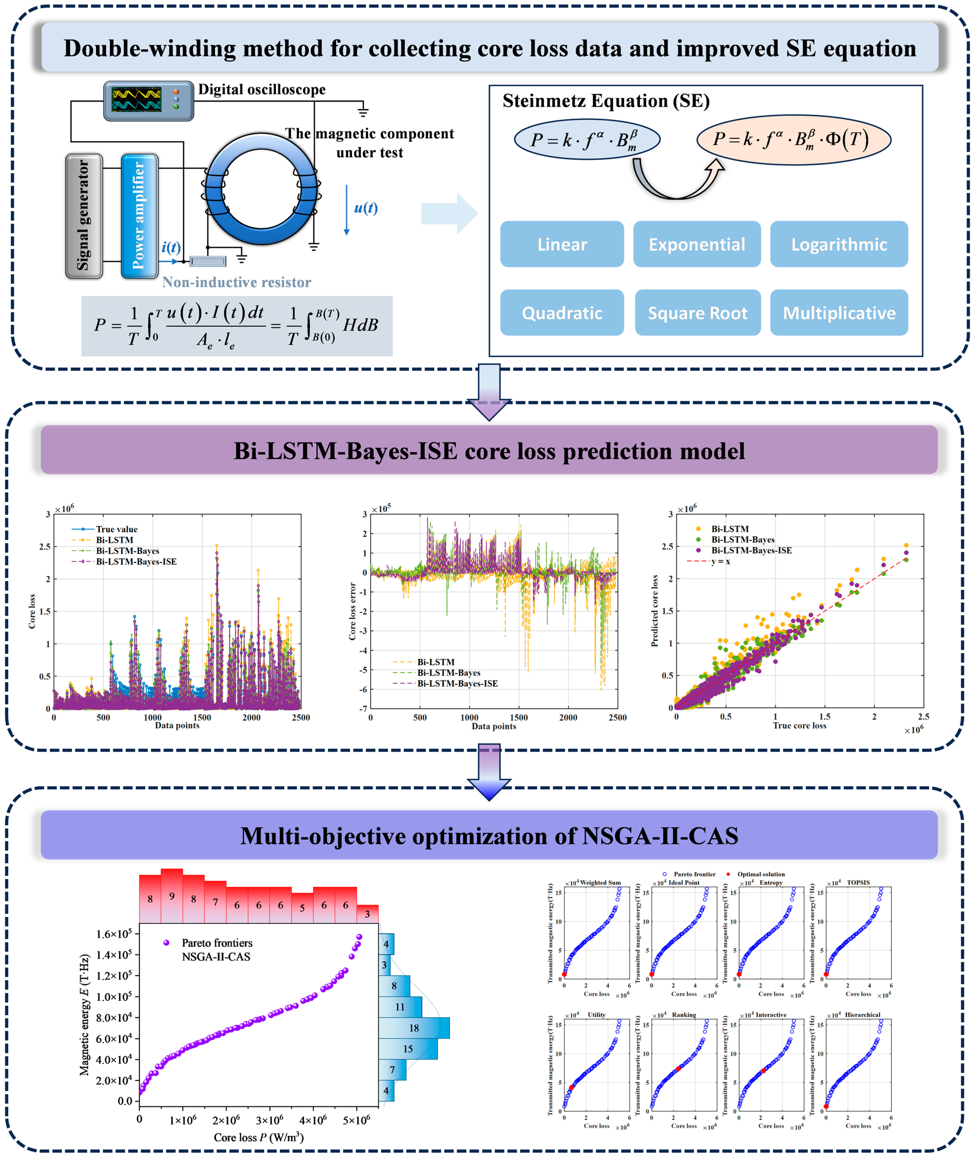
This study proposes a comprehensive prediction and optimization framework (Figure 3) to explore the optimal trade-off point between minimum loss and maximum energy efficiency, and to guide the selection of magnetic materials and the adjustment of working parameters in different application scenarios. Firstly, the SE equation and the optimization of its improved equation considering temperature were discussed. Then, based on the Bi-LSTM-Bayes-ISE core loss prediction model and combined with the measurement index of transmission magnetic energy, a comprehensive optimization model for core loss prediction optimization based on the NSGA-II-CAS algorithm is established. By analyzing the influence of multiple variables, the optimal conditions are identified.

2.5. Materials and Data Preprocessing

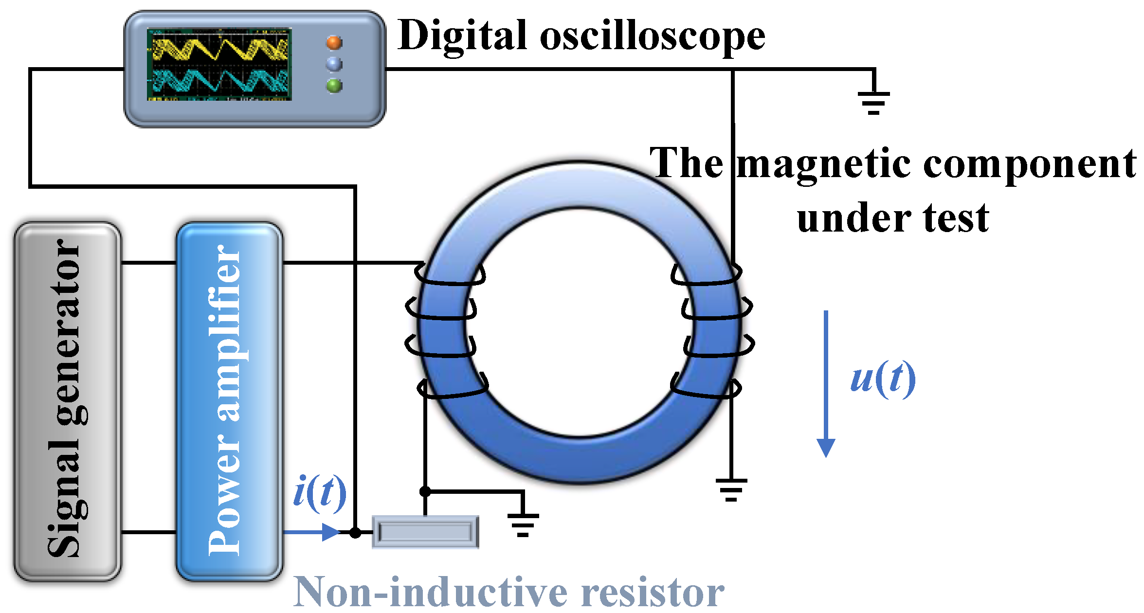
Core loss characterization commonly employs the AC power method, with the experimental setup depicted in Figure 4. The toroidal core (mean magnetic path length le, cross-sectional area Ae) is equipped with dual symmetrically wound coils (N1 = N2 turns). A signal generator produces sinusoidal/arbitrary waveforms at frequency f (period T = 1/f), amplified by a high-frequency power amplifier before driving the excitation coil.
Governed by Ampère’s Law, the excitation current I(t) generates magnetic field strength H(t) = N1I(t)/le (magnetomotive force per unit length). Concurrently, time-varying B(t) (magnetic flux density) is induced per Faraday’s Law, producing measurable voltage in the sensing coil. Simultaneous acquisition of I(t) and sensing voltage u(t) enables H(t)/B(t) waveform reconstruction for core loss density calculation (Equation (25)), with B(t) characteristics serving as operational state indicators.
P = 1 T 0 T u t I t d t A e l e = 1 T B 0 B T H d B
The dataset adopted in this study (Table 2) includes material, temperature, frequency, core loss, excitation waveform, and magnetic flux density time series of 1024 sampling points in each group. The dimensions of the four different material datasets are 3400 × 1028, 3000 × 1028, 3200 × 1028, and 2800 × 1028 respectively, among which the materials (four types) and excitation waveforms (sine, triangle, and trapezoid) are label data. Source of data set for the 21st session of Chinese graduate students mathematical contest in modeling problem C public data sets (https://cpipc.acge.org.cn/cw/detail/4/2c90801791c6c0a80191f9a6b0366533, accessed on 21 September 2024). The original source of this dataset is the MagNet open-source database [36,51]. The database was jointly developed and established by Princeton University and Dartmouth College. The excitation waveforms have been classified according to the waveform characteristics of the magnetic flux density time series. Considering the transparency of the data, all data can be directly obtained from the official links. In this study, only the statistical data characteristics of all four different material types are presented as shown in Table 2. While the dataset provides comprehensive multi-material coverage, two limitations warrant attention: The excitation waveform classification relies on predefined flux density characteristics, which may not capture all real-world variations.
The collection of this dataset was carried out using the double-line method (Figure 4), and the quality of the dataset was strictly controlled by the official and authoritative organizing committee of the China Postgraduate Mathematical Modeling Contest. At the same time, considering the occurrence of errors, while modeling and predicting, we adopted the 3sigma (3σ) method to handle outliers on the data in the dataset. We excluded a very small number of core loss data samples that did not meet 3σ. According to the calculation of sigma based on Equation (26), it can be known that the probability of the data distribution within the 3sigma interval (μ − 3σ, μ + 3σ) is 99.73%.
μ = 1 n i = 1 n x i σ = i = 1 n x i μ 2 n
where n is the sample quantity, xi is the core loss, μ is the average core loss of all samples, and σ is the standard deviation of the core loss of all samples.

3. Results and Discussion

3.1. Core Loss Coefficient Fitting and Temperature Correction Equation

3.1.1. Coefficient Fitting of the SE Equation

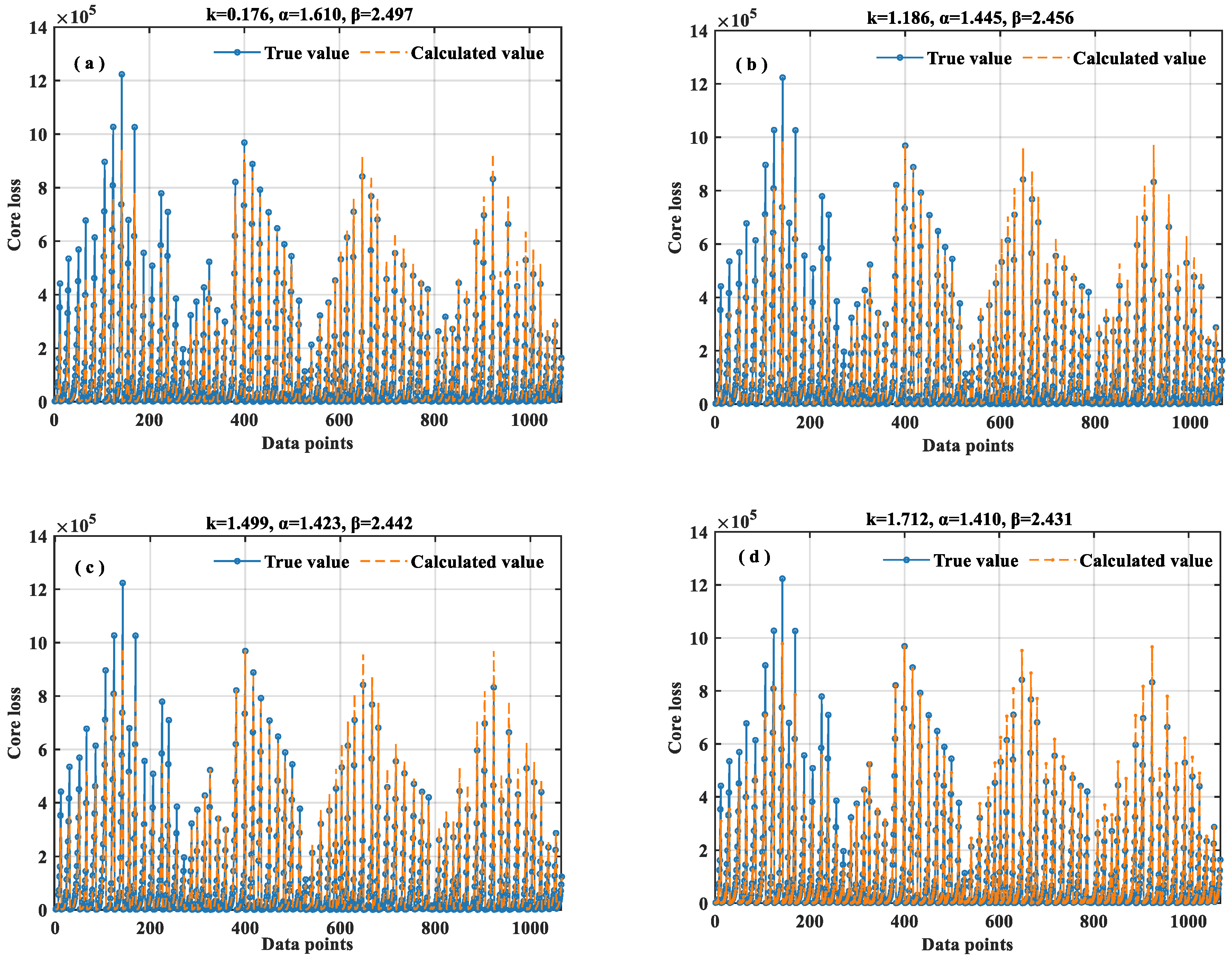
In order to study the temperature correction scheme of the SE equation under the condition that the magnetic waveform is sinusoidal, the coefficients are fitted first. By analyzing the existing experimental data, without considering the influence of temperature, k, α, and β of the SE equation are fitted using f and Bm. The fitting results are shown in Figure 5.
The four fitting methods adopted are linear fitting, nonlinear least square method, annealing algorithm, and genetic algorithm. Among them, the linear fitting method is simple and has a small computational load, but it has poor adaptability to nonlinear relationships. The nonlinear least square method is suitable for complex nonlinear relationships and performs parameter fitting by minimizing the error square. Annealing algorithms and genetic algorithms are applicable to multimodal optimization problems, which can avoid local optima, but they have relatively high computational complexity. For the four proposed methods, f and Bm are used as inputs to fit the core loss and find the optimal coefficient. In Figure 5, the fitting results of the four methods are relatively close. The predictions for the first 500 or so data points are all smaller, while the predicted values after 500 are larger than the true values. The core losses obtained after fitting by four methods were evaluated and the errors were analyzed. The error results of core loss calculated by four methods are shown in Table 3.
The MaxError, MSE, RMSE, and MAE of the nonlinear least squares method are all the smallest (Table 3), while it has the largest R2 (0.9455). The calculation results of the annealing algorithm are similar to those of the nonlinear least square method, but the local errors are relatively large. Therefore, among the four methods, the nonlinear least square method has the best fitting effect. The nonlinear least squares fitting process adopts the Levenberg–Marquardt algorithm and the Gauss–Newton method and has better convergence performance for nonlinear problems.

3.1.2. ISE Equation and Verification

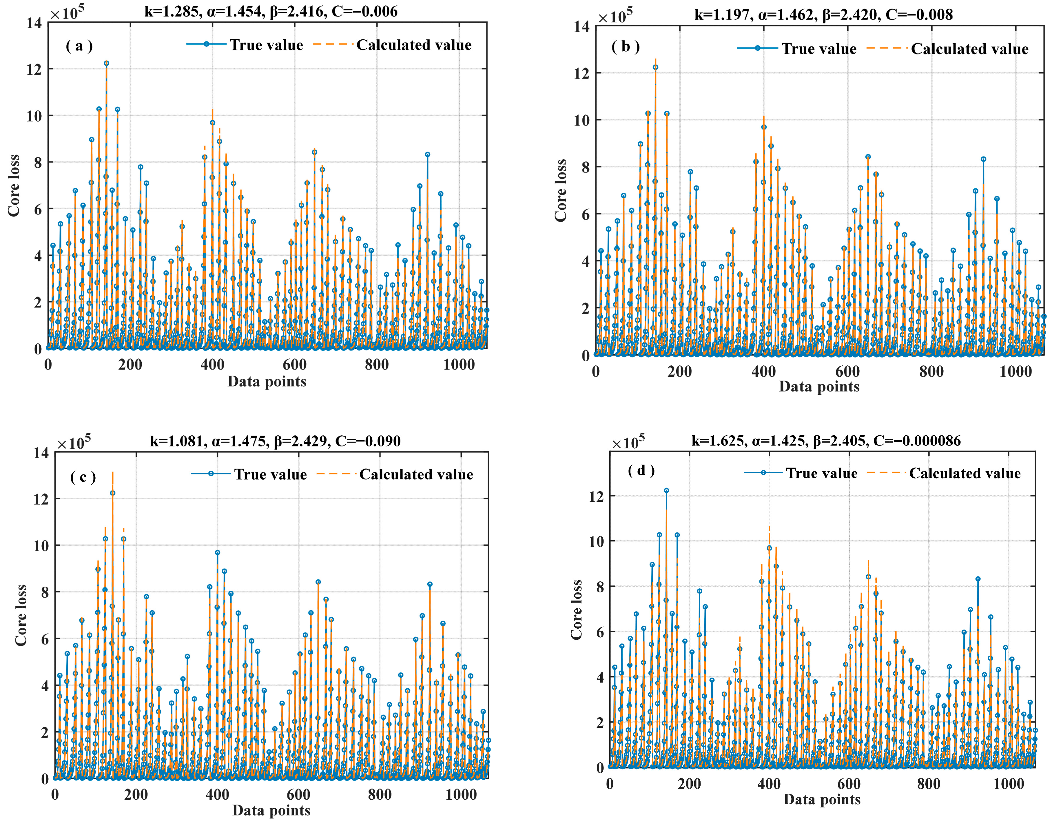
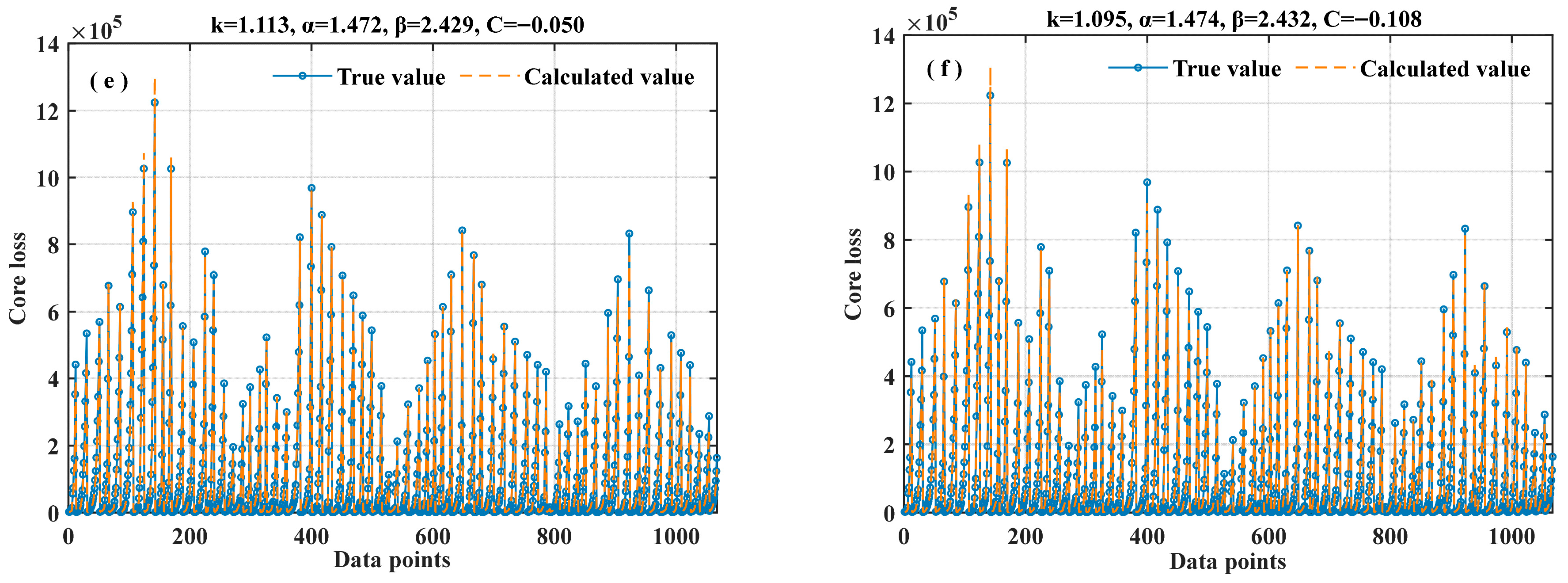
Based on the nonlinear least squares method for optimal coefficient fitting of the core loss model, the accuracy of core loss prediction is further improved. Different temperature correction forms are adopted, and the temperature factor is taken into account in the SE equation to enhance the calculation accuracy of core loss. Taking the sinusoidal waveform data in Material 1 as the analysis object, the modified equation considering temperature constructed was applied to the same data set to calculate the modified predicted value of core loss. Compare the errors between the SE and ISE, and evaluate the improvement effect of the modified equation in predicted value. According to the six modified equations proposed in Section 2.1.2, the equation coefficients were re-fitted, and the fitting results are shown in Figure 6.
The results of core loss calculated by various correction methods after introducing temperature as a variable for correction are all closer to the true value (Figure 6). Among them, the overall visual effect of square root correction and multiplication correction is better. Error analysis was conducted on six correction methods to screen out the one with the best correction effect. Table 4 presents the performance analysis results of core loss calculation for different correction methods.
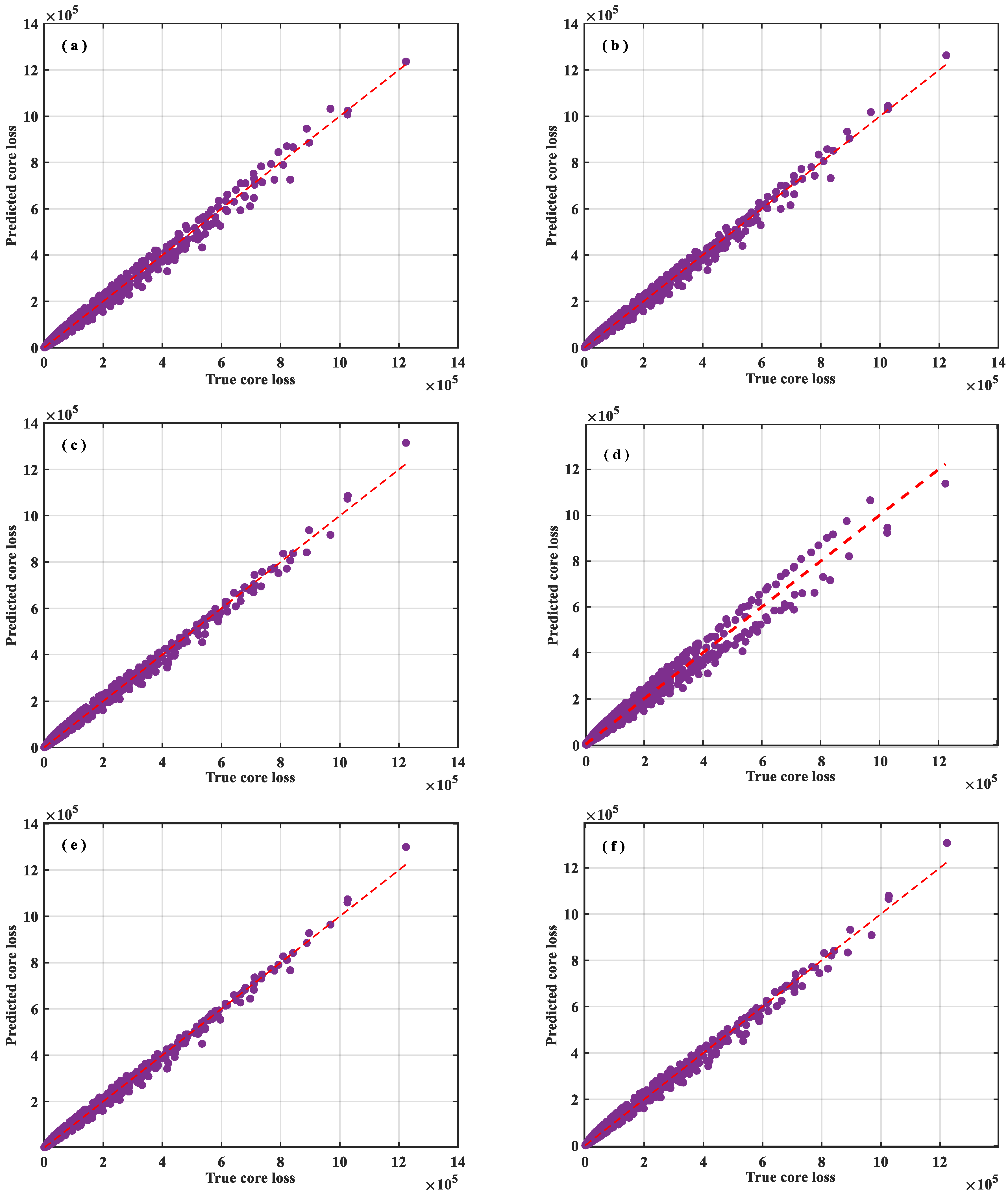
The error generated by linear correction is much higher than that of the other five methods, and the effect is average (Table 4). The errors of exponential correction and logarithmic correction are relatively low, and the R2 values are high, with better effects. The square correction error is relatively large, and the R2 value is also relatively low, making it the method with the worst correction effect among all methods. Among all the square root correction error indicators, it is the lowest, and the R2 value (0.9954) is the highest, which is the best effect among all the methods. The effect of multiplication correction is similar to that of square root correction. The R2 value (0.9937) is slightly lower than that of the square root correction method, and its effect is second only to that of the square root correction. To analyze the effects of the six correction methods more intuitively, the results were visualized using kernel density plots. The kernel density plots of the six methods are shown in Figure 7.
It can be seen from Figure 7 that the fitting accuracy of the square correction method is the worst, and the data has shown discrete bifurcations. The core loss calculated by the square root correction method has a higher fitting accuracy with the real core loss curve, which proves that the core loss temperature correction model using the square root correction method has the best effect. The square root obtained so far is 1/2 of the temperature, which is not necessarily the optimal parameter. Therefore, the correction effects of both linear correction and quadratic correction methods are weaker than those of the square root correction method.
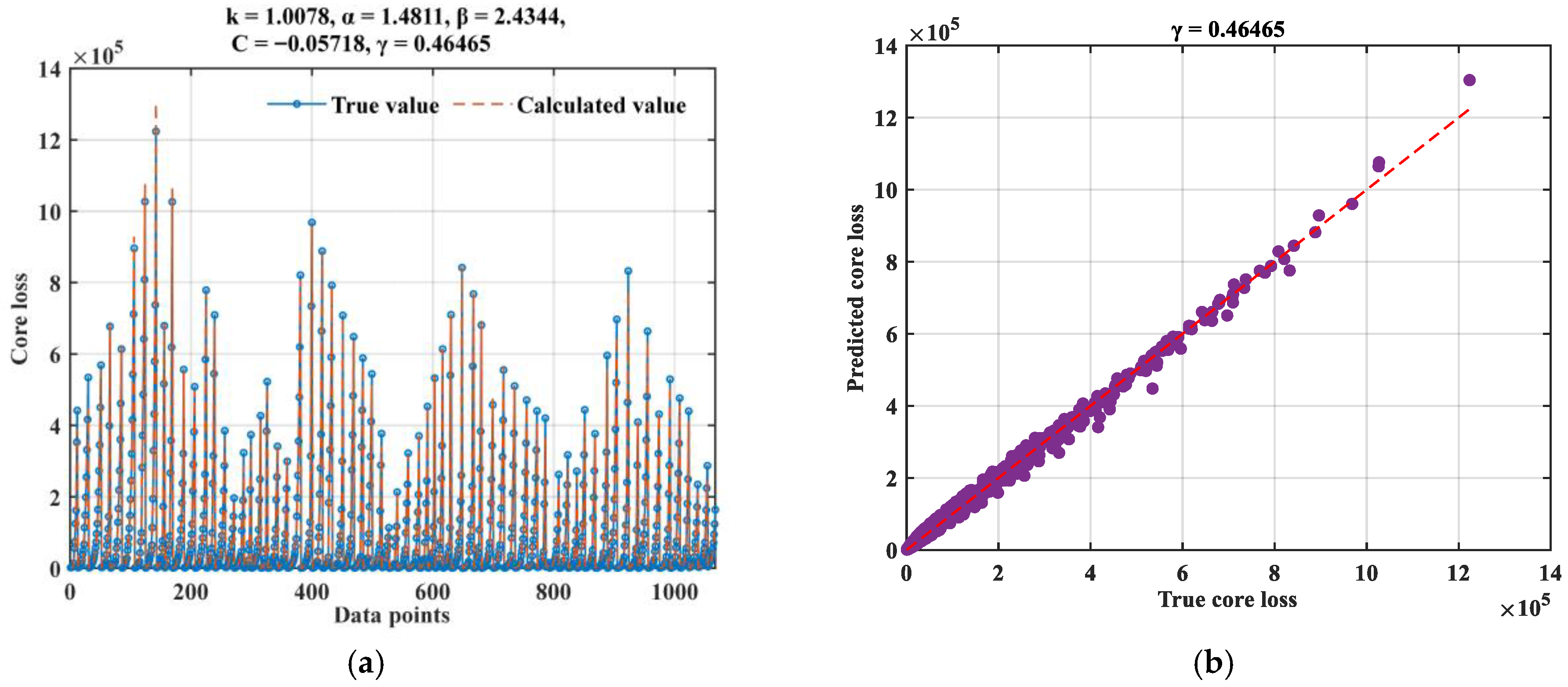
Based on the proposed core loss temperature correction model using the square root correction method, the exponential power of the temperature is further optimized. Let the exponential power of the temperature be the coefficient γ (ranging from 0 to 1) for parameter optimization (Figure 8 and Table 5).
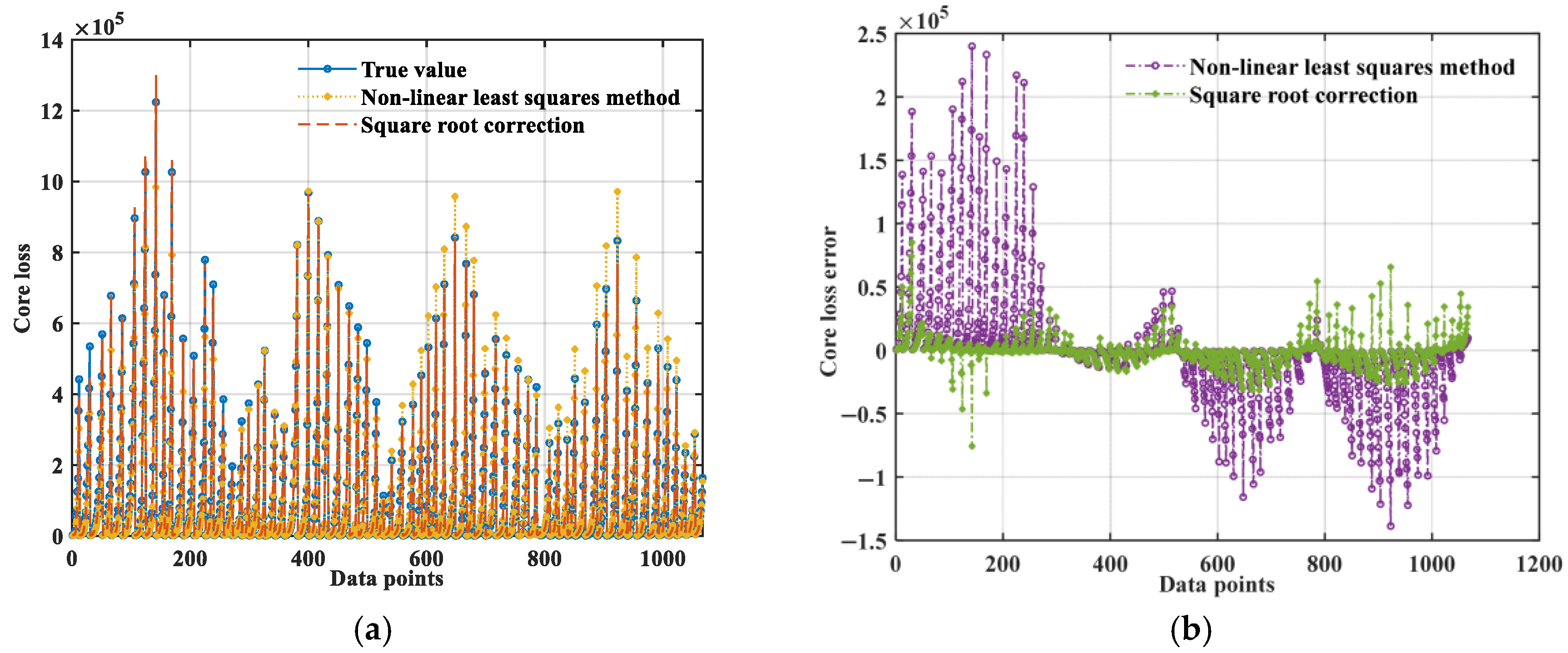
It can be seen from the result analysis in Table 5 that optimizing the value of the exponential power can slightly improve the model accuracy, but the optimized equation is not conducive to calculation (with an exponent of 0.46465). Considering the actual situation, we need to reduce the computational complexity. The square root (with an exponent of 0.5) correction model is still adopted. The core loss after fitting the SE equation by the nonlinear least square method, the core loss after fitting the SE equation by square root correction considering the temperature factor (ISE), and the actual core loss value are compared as shown in Figure 9. When the temperature factor is not considered, the core loss fitted by the nonlinear least square method still deviates significantly from the true value. After temperature correction by the SE equation, the calculated value of the core loss is significantly closer to the true value, which proves the correctness of the core loss temperature correction model adopted. It can adapt to different temperature changes and make the prediction effect of core loss better.

3.2. Core Loss Prediction Based on Bi-LSTM-Bayes-ISE

3.2.1. Bi-LSTM

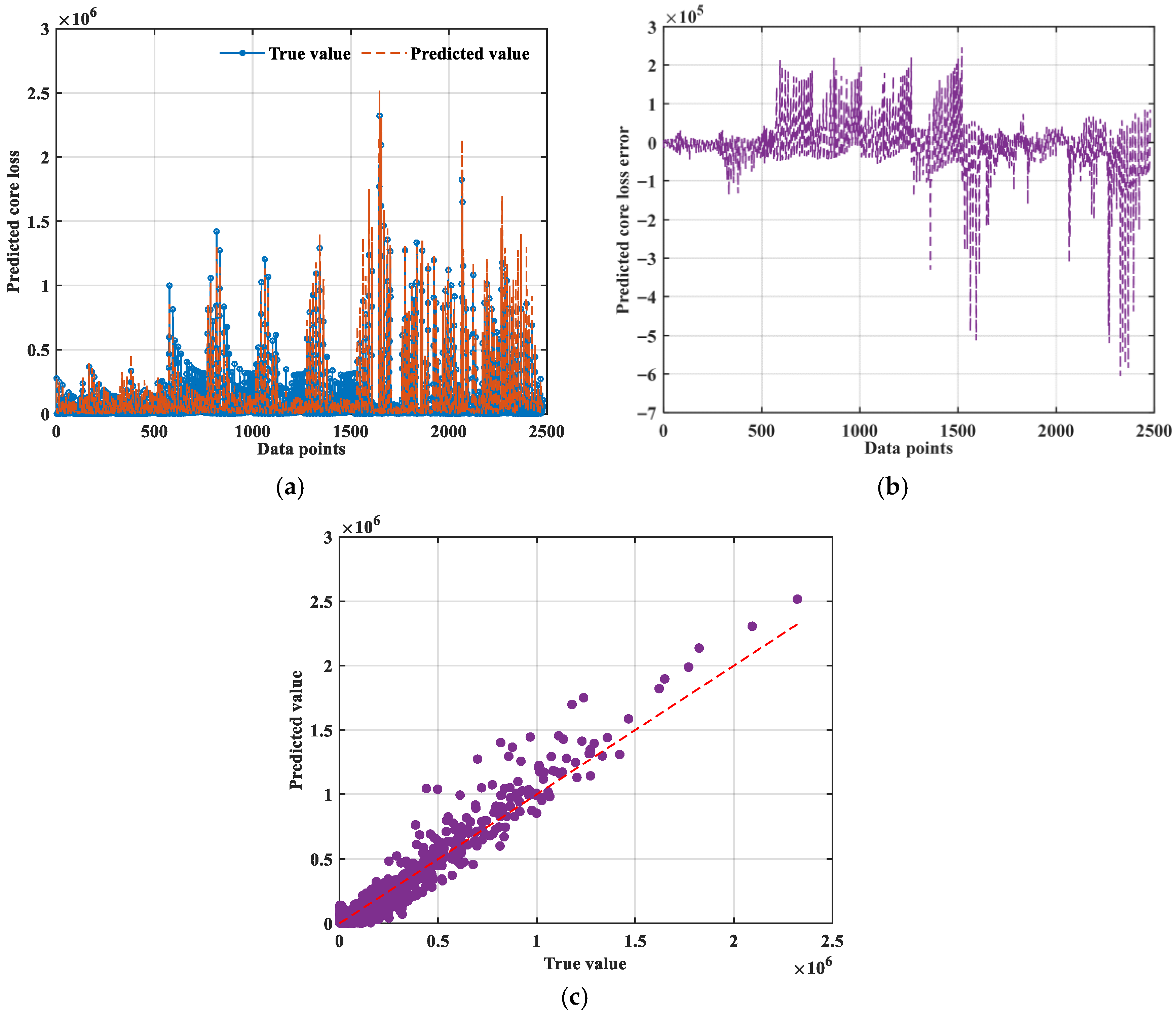
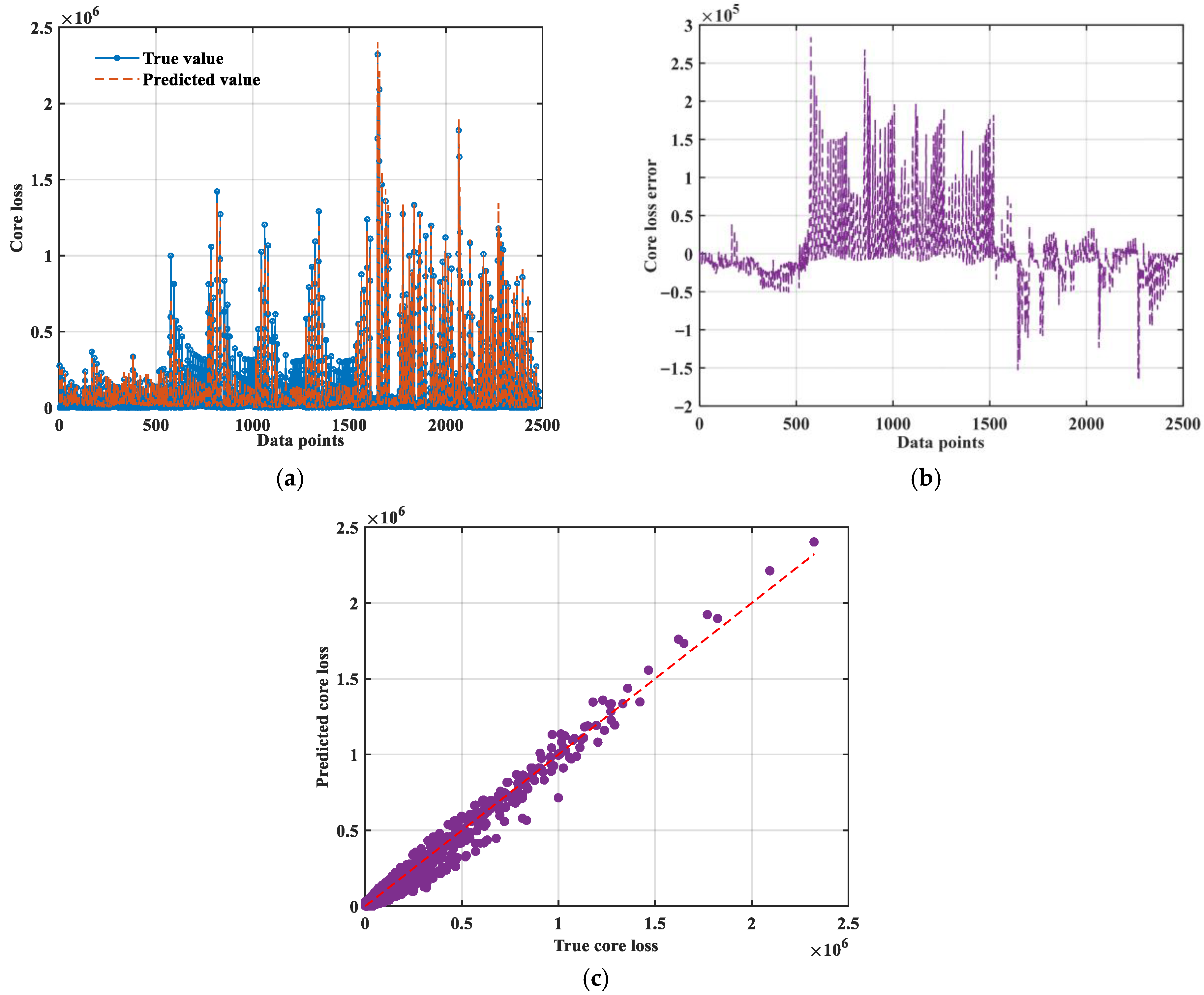
The establishment of a core loss prediction model based on Bi-LSTM deep learning is a process involving the processing of complex data sequences. Core loss is closely related to factors such as material type, temperature, and excitation waveform, and these data usually exhibit significant time series characteristics. Therefore, Bi-LSTM is highly suitable for predicting core losses. Figure 10a presents the comparison results between the predicted values and the true values of core loss by the Bi-LSTM deep learning algorithm. Figure 10b shows the statistics of the error values of core loss. Figure 10c presents the visualization processing results of the kernel density of the predicted values.
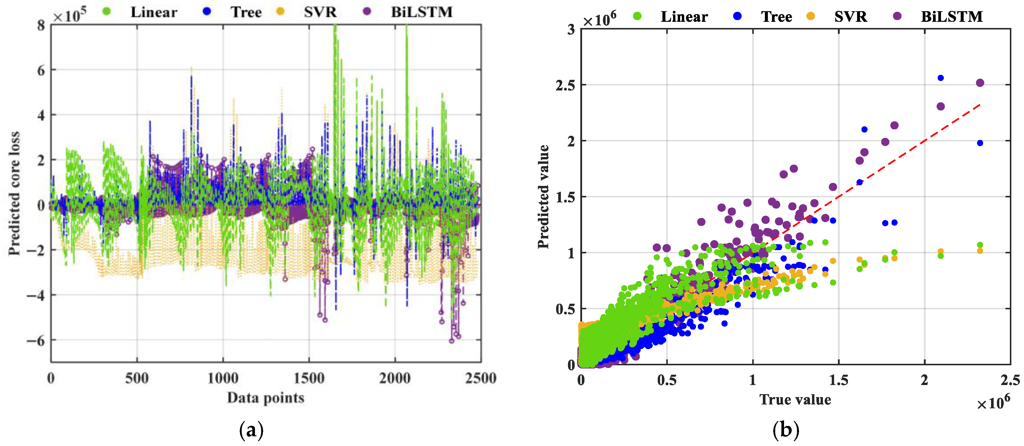
From the comparison results of the true values and predicted values of the core loss prediction model in Figure 10a, it can be seen that there is a certain error especially for some data points between 1500 and 2500. The error values is relatively large. Meanwhile, according to the kernel density graph of the predicted core loss values, it can be seen that the data points are relatively discrete and the fitting accuracy is poor. Figure 11 presents the analysis results of core loss performance and error based on Bi-LSTM and three basic machine learning models. The prediction error of Bi-LSTM is smaller than that of Linear, SVR, and Decision Tree (Figure 11a). It can be seen that the values of RMSE, MSE, MAE, and SMAPE are relatively large. Although Bi-LSTM performs better than other basic models, there is still room for improvement, which inspires us to expand further optimizations (such as Section 3.2.2 and Section 3.2.3).
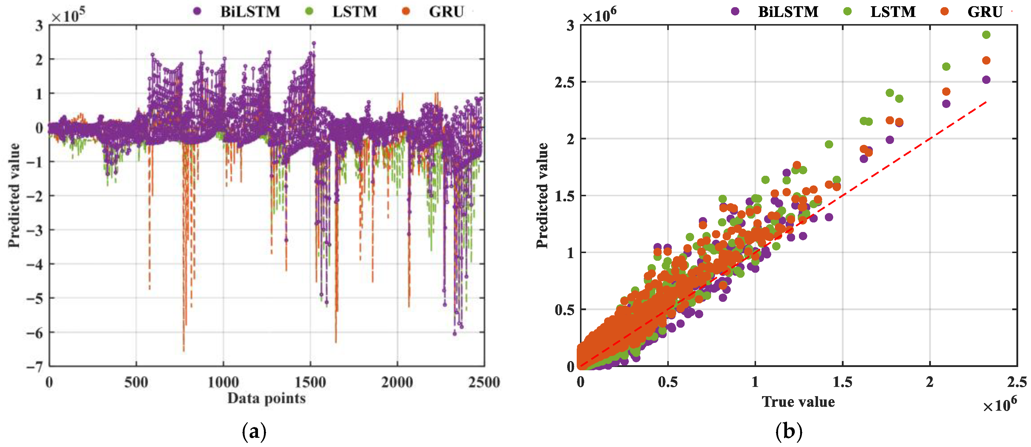
Furthermore, we also conducted a comparative analysis of the Bi-LSTM model with other classic deep learning models (LSTM, GRU), as shown in Figure 12. Bi-LSTM is closest to the 1:1 error line in both Figure 11b and Figure 12b, indicating that the error gap is the smallest. The performance results of all the basic models are presented in Table 6. Based on the comprehensive performance results, Bi-LSTM has the largest R2 and the best performance, and can be considered as the basic model for core loss prediction.

3.2.2. Bi-LSTM-Bayes

Because the predicted values obtained by the core loss prediction model based on Bi-LSTM still have a certain error compared with the true values, the Bayesian method is adopted to optimize the model. Bayesian hyperparameter optimization aims to automatically adjust the hyperparameters of the model to improve its performance. Table 7 presents the parameter range and the optimal hyperparameters for Bayesian hyperparameter optimization, including the number of hidden units, learning rate, maximum training number, and batch size.
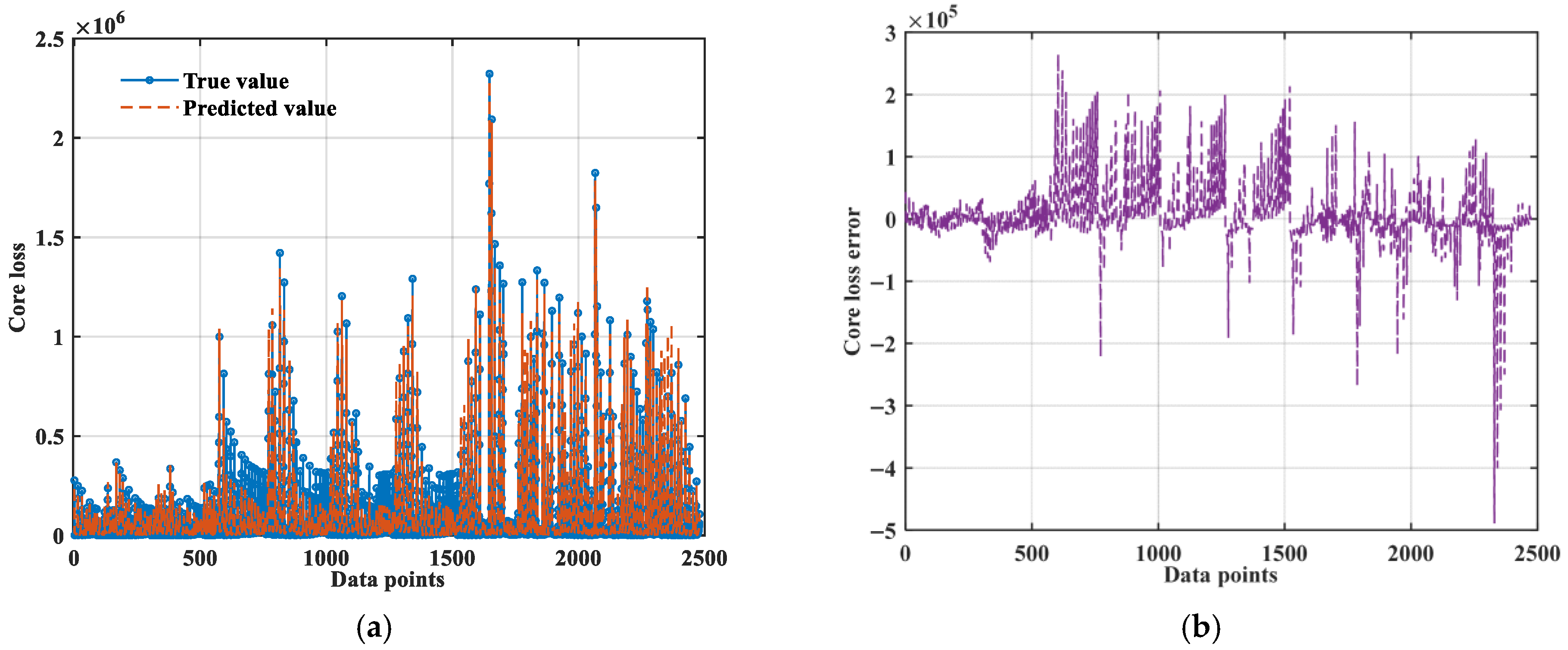
Based on the optimal hyperparameters obtained from the optimization of Bayes hyperparameters, the Bi-LSTM-Bayes core loss prediction model is constructed below and compared with the real values. Figure 13 presents the comparison result between the predicted value and the true value of core loss. The accuracy of the prediction model corrected with the optimal hyperparameters has been significantly improved (compared with Figure 10). In particular, the error values of some data points from 1500 to 2500 have been significantly reduced.
Table 8 presents the error analysis results based on the Bi-LSTM-Bayes core loss prediction model. Compared with Table 6, the RMSE, MSE, MAE, and SMAPE values have generally decreased, and the R2 value of the Bi-LSTM-Bayes model has also increased (reaching 0.9568, an increase of approximately 6%). It can be seen that after Bayesian hyperparameter optimization, the accuracy of the core loss model has been significantly improved. Compared with LSTM, GRU, SVR, Decision Tree, and Linear, Bi-LSTM shows relatively better performance whether it is optimized by Bayes or not.

3.2.3. Bi-LSTM-Bayes-ISE

Although the accuracy of the core loss model based on Bi-LSTM has been improved after Bayesian hyperparameter optimization, the physical model based on the aforementioned SE modified equation also has high prediction accuracy and a high-precision function model. Therefore, based on the Bi-LSTM-Bayes core loss prediction model, the physical model of the ISE is considered as an input feature supplement to optimize the prediction model. Figure 14 presents the results of the Bi-LSTM-Bayes-ISE core loss prediction model, the statistics of the error values, and the visualization results of the kernel density.
The accuracy of the prediction model optimized by the ISE physical model has been significantly improved, and the error values have been significantly reduced (Figure 14). Table 9 presents the performance analysis results based on the Bi-LSTM-Bayes-ISE core loss prediction model. Compared with Table 8, the values of RMSE, MSE, MAE, and SMAPE were further reduced, and the R2 value was also increased (reaching 0.9622). It can be seen that after considering the ISE physical model, the prediction accuracy of the core loss model has been further improved.
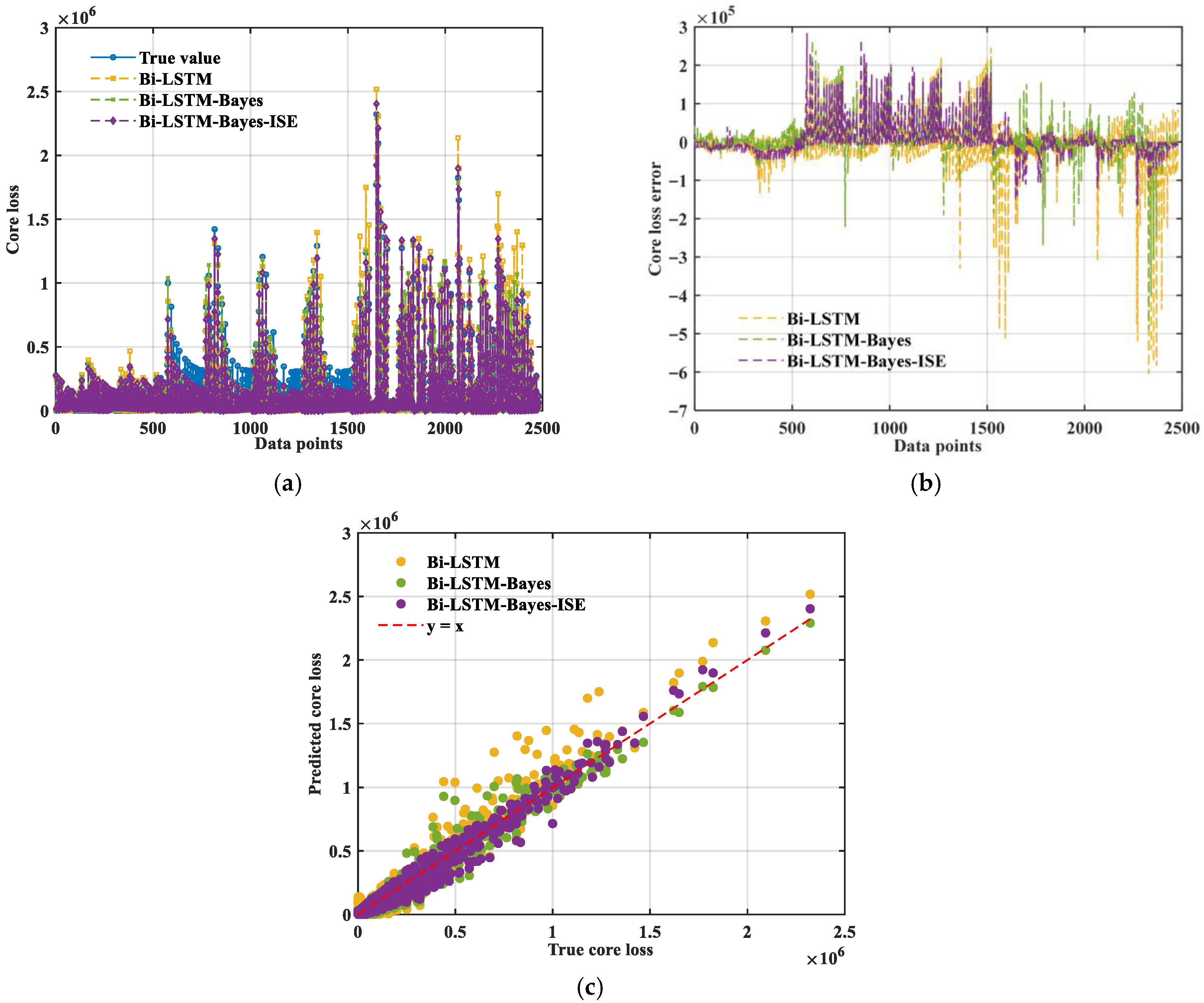
The predicted values of the core loss prediction models of Bi-LSTM, Bi-LSTM-Bayes, and Bi-LSTM-Bayes-ISE were compared with the true values, and the results are shown in Figure 15. Before the Bayesian hyperparameter optimization, the predicted core loss based on Bi-LSTM deep learning still deviated greatly from the true value. After the hyperparameter optimization, the calculated value of the core loss was significantly closer to the true value, which proved the correctness of the hyperparameter optimization. After introducing the ISE modified equation, the accuracy of the prediction model was further improved, making the best predicted results.

3.3. Core Loss Prediction Optimization Based on NSGA-II-CSA

Multiple objectives to be solved need to be transformed into solvable extremum objective functions. Firstly, the objective functions regarding P and E are defined as follows:
Min   P   =   g T , f , W , B m , M
Max   E = f × B m
where P is the core loss; g(·) is a function of P; E is the transmitted magnetic energy, and T, f, M, W, and Bm are, respectively, the temperature, frequency, material type, excitation waveform type, and peak magnetic flux density. Meanwhile, these decision variables need to meet the following conditions:
S . t   T = 25 , 50 , 70 , 90 f 49990 , 501180 W = s i n e , t r i a n g l e , t r a p e z o i d = 1 , 2 , 3 M = M a t e r i a l 1 , M a t e r i a l 2 , M a t e r i a l 3 , M a t e r i a l 4 = 1 , 2 , 3 , 4 B m 0.0096 , 0.3133
The NSGA-II algorithm randomly generates a series of initial populations of a certain scale based on the search space and constraints of the problem. This population contains the starting point of algorithm optimization, and each individual represents a potential solution. Furthermore, non-dominant sorting is carried out based on the dominance relationship to divide multiple Pareto front. Then, a series of crowding degree calculations (such as the sum of total distances, see Equation (30)), selection of crowding comparison operators, crossover and mutation (such as individual c mutation, see Equation (31)), population mutation, and update are carried out until the maximum population convergence or the maximum algebra G is reached.
d i = k = 1 m d i k = k = 1 m f k i + 1 f k i 1 f k max f k min d 1 k = d N k =
δ m = 2 u 1 / n m + 1 1 , if   u < 0.5   1 2 1 u 1 / n m + 1 , if   u 0.5 c i = c i + δ m c i max c i min
where di is the total congestion distance, u is a uniformly distributed random number, and nm is the mutation release index.

3.3.1. Pareto Front

Based on the NSGA-II algorithm, the Bi-LSTM-Bayes-ISE core loss prediction model was adopted as the core loss function objective, and MOO training was carried out. The parameter selection of related algorithms will affect the number of selected Pareto frontiers and the degree of training. Referring to the current data volume and operating costs, the algorithm parameters are shown in Table 10.
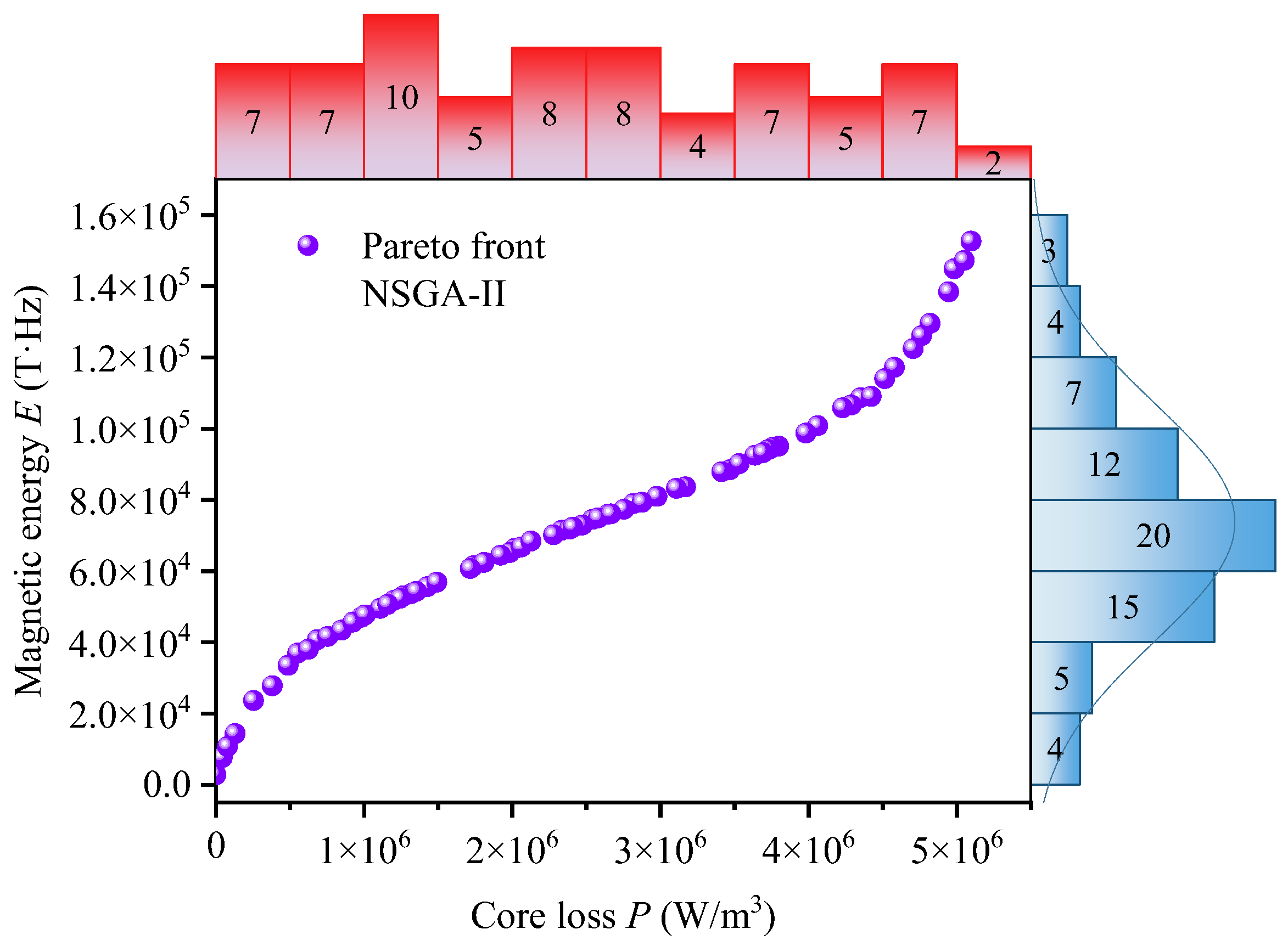
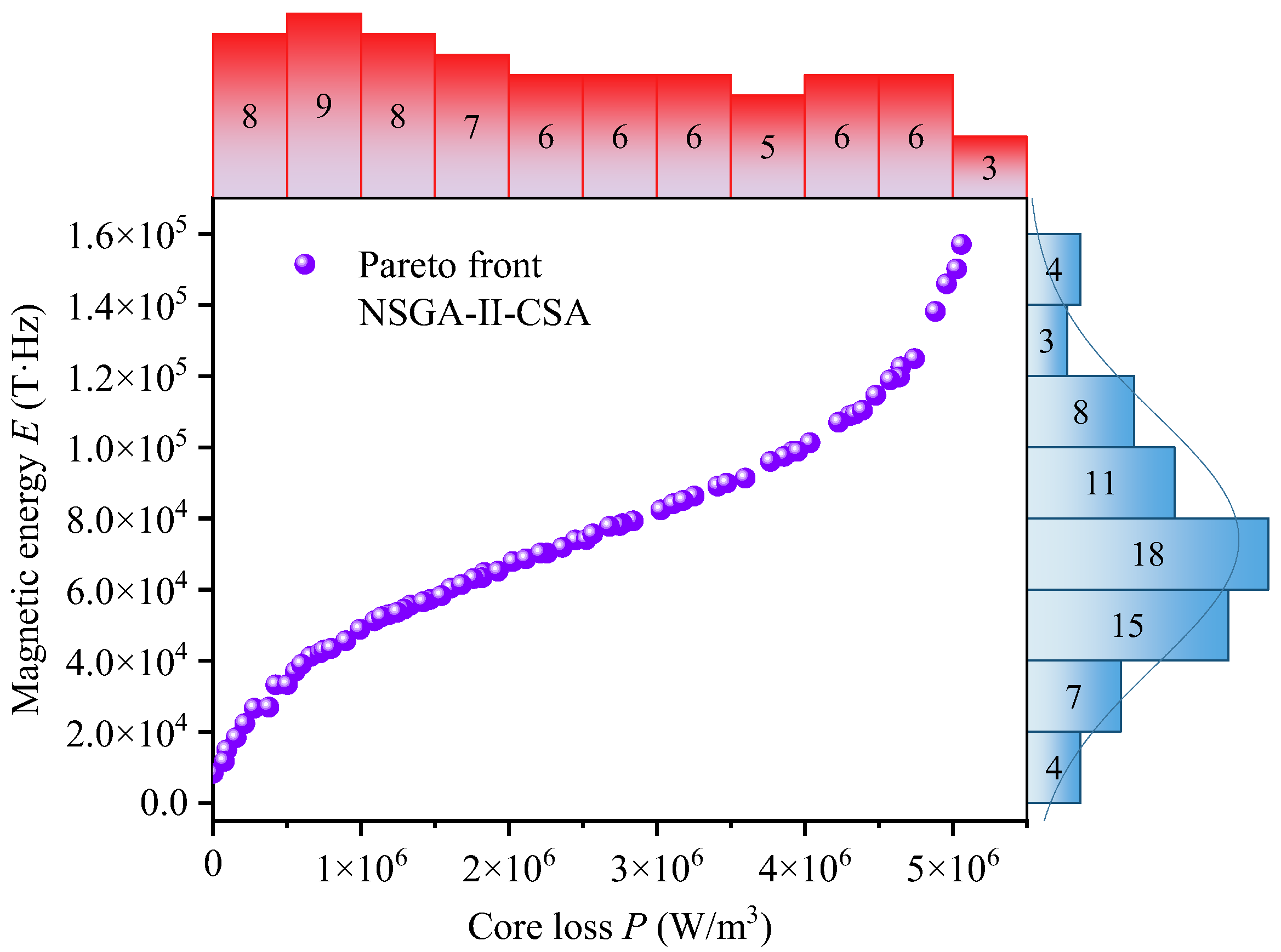
Taking into account P and E comprehensively, the Pareto front diagram of the optimization result is shown in Figure 16. It shows 70 Pareto frontier values, represented by a “gradient red” to indicate the frequency distribution histogram of the related core losses, highlighting the negative impact of core losses on magnetic components. Correspondingly, the frequency distribution histogram of the relevant transmitted magnetic energy is represented by “gradient blue” to demonstrate the positive effect of the transmission magnetic energy. The magnetic flux loss distribution corresponding to the value of the optimal solution is uniform, and the transmission magnetic energy shows a normal distribution law.

3.3.2. Optimal Condition Solution Based on Eight Decision-Making Methods

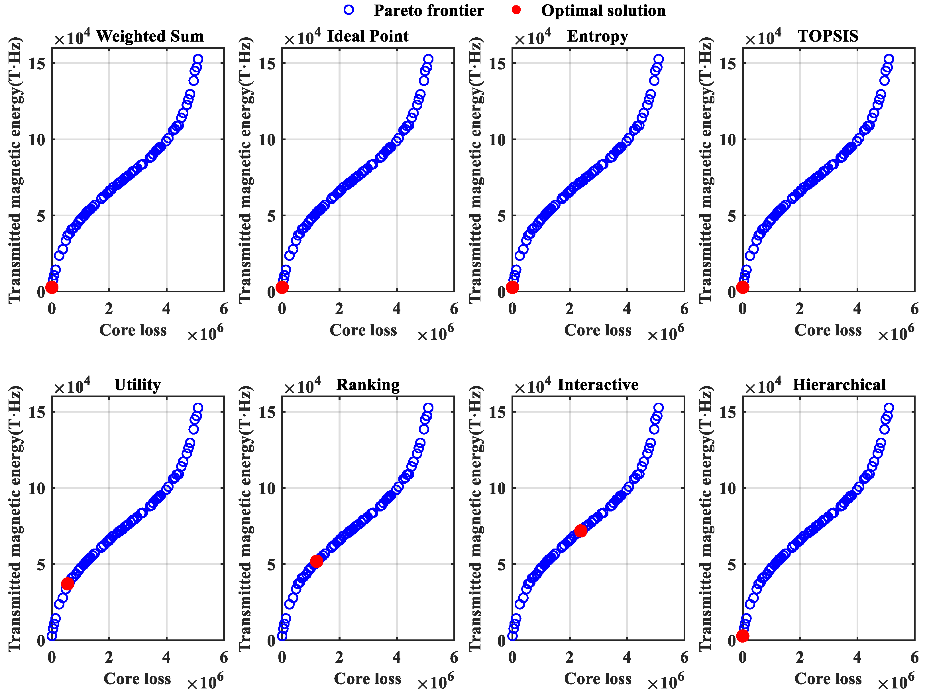
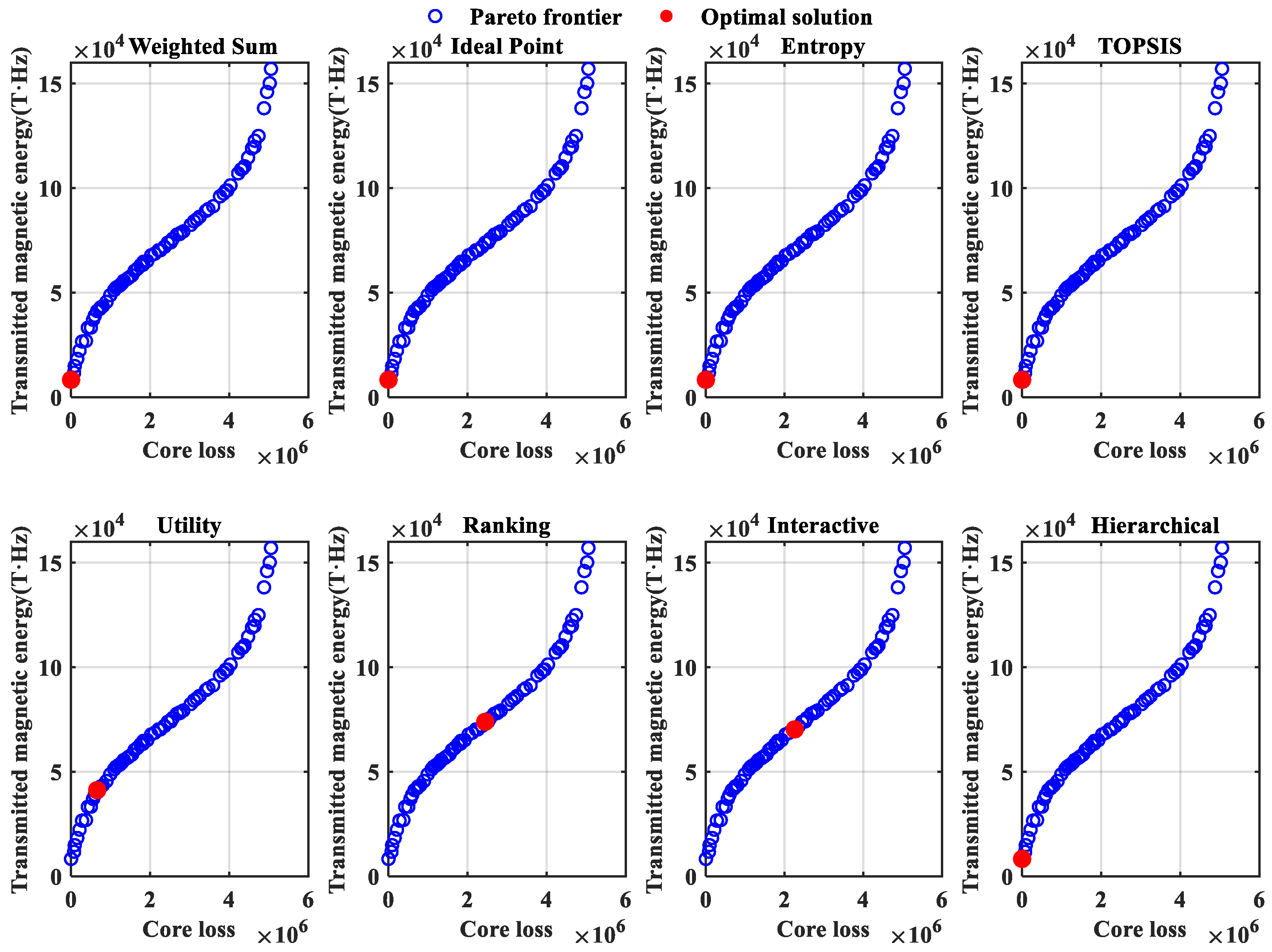
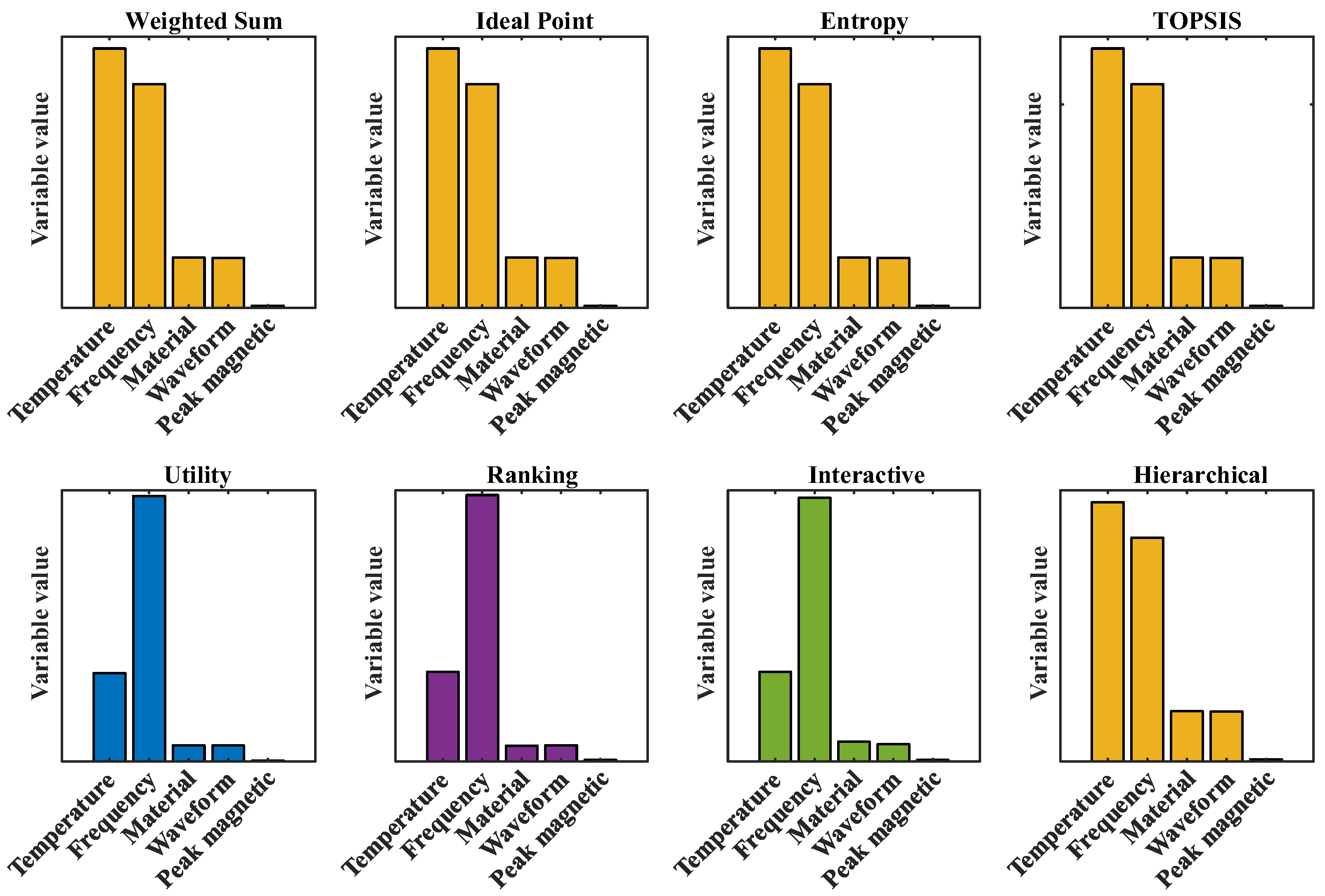
Figure 17 shows the selection of the optimal solution for eight decision-making methods. Among them, WSM, IPM, EWM, TOPSIS method, and HOM have selected the same point under the default setting conditions, where both the core loss and the transmitted magnetic energy are at the lowest values. This is obviously not the most suitable optimal solution.
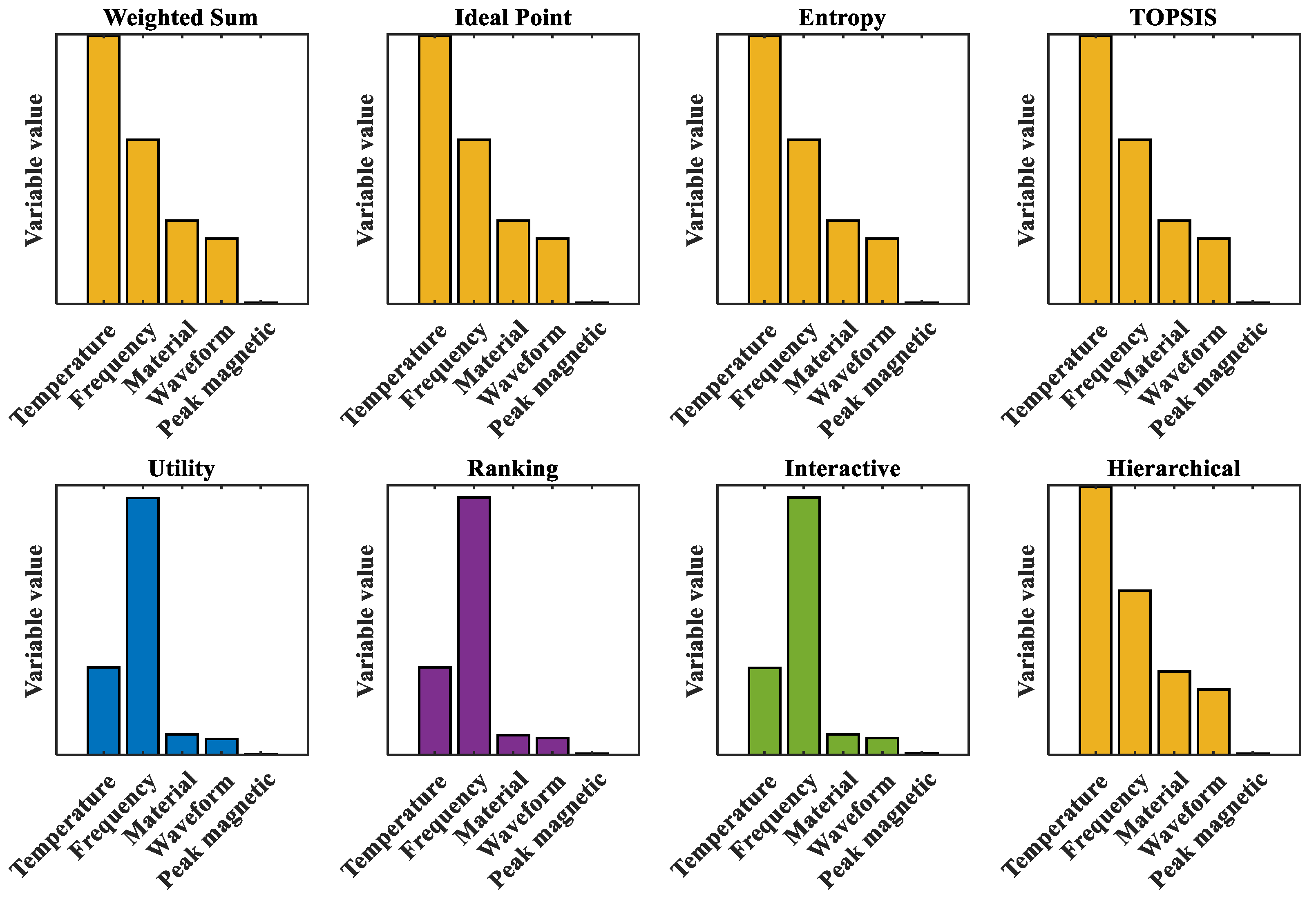
Taking into account the scattered point distribution in Figure 17 comprehensively, the optimal solution selection of UFM, RBSM, and IM would be more appropriate. The optimal solutions and influencing factors for all eight types of decision-making methods are selected (Table 11 and Figure 18), respectively. The optimal solutions selected by WSM, IPM, EWM, TOPSIS method, and HOM are only theoretically reasonable. Although the core loss (22.71 W/m3) is very low, the actual magnetic energy is only 0.00036 T·Hz. On the contrary, the optimal solutions of UFM, RBSM, and IM are more suitable for the actual requirements of magnetic components. These three optimal solutions are all sinusoidal waves, material 1, and 90 °C, with specific frequencies all around 470,000 Hz. The peak magnetic flux densities are different, and the corresponding core losses and transmitted magnetic energy basically maintain a positive correlation state.

3.3.3. NSGA-II-CSA

Based on the NSGA-II-CSA model, Figure 19 shows the Pareto front results calculated by the improved model. It can be seen from the figure that the relevant scattered points are concentrated. Especially when the core loss is between 106 and 2 × 10⁶ W/m3 and the transmitted magnetic energy is between 4 × 10⁴ and 6 × 10⁴ T·Hz, the number of Pareto frontiers reaches 30.
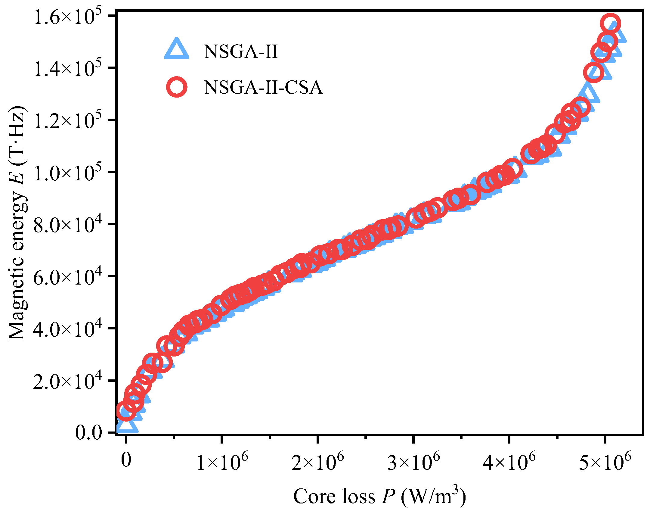
To further compare the model effects before and after optimization, a Pareto front scatter comparison chart before and after improvement was drawn (as shown in Figure 20). From the comparison chart, it can be seen that the similarity of the relevant optimal condition solution sets is relatively large, and the overall deviation is small. However, we can find that the Pareto front after CSA optimization is more concentrated in the middle of the two objectives, and the number of solutions in the lower left and upper right corners of Figure 20 is sparser. It is impossible to determine the optimal solution merely from the solution set graph. At this time, eight optimization strategies are necessary. The optimal conditions of the NSGA-II-CSA model were solved by using the same eight decision-making methods, and the multi-decision optimal solution selection graph was drawn as shown in Figure 21.
Through these eight types of methods, decisions can be made to select the optimal conditions. To further understand the relevant optimal solution values, we have supplemented Table 12 and Figure 22 to demonstrate the optimal conditions of the NSGA-II-CSA algorithm. According to the optimal decision conditions in Table 12, the magnetic components selected under 90 °C, material 1, and sine wave conditions can approach the optimum in terms of core loss and transmission magnetic energy.
For the specific selection of the optimal solution, refer to the bolded part in Table 12. The scientific analysis of optimal solution selection based on UFM, RBSM, and IM methods reveals critical trade-offs between core loss minimization and magnetic energy transmission maximization. UFM achieves the lowest core loss (659,555 W/m3) while simultaneously maximizing transmitted magnetic energy (41,201.9 T·Hz). This dual superiority suggests UFM effectively balances the conflicting objectives of loss reduction and energy efficiency.
UFM operates at lower frequency (489,674 Hz) and peak flux density (0.0841 T) compared to RBSM and IM. These conservative parameters likely reduce hysteresis/eddy current losses while maintaining sufficient energy transmission through optimized waveform utilization. RBSM and IM use higher flux densities (0.1445–0.1504 T) and frequencies (486,189–491,283 Hz), which increase energy transmission but at the cost of significantly higher core losses (3.7–3.8× UFM’s loss). UFM’s utility function framework appears to capture nonlinear relationships between operational parameters more effectively than ranking-based (RBSM) or interactive (IM) approaches. This enables simultaneous optimization of multiple objectives without requiring predefined weights or iterative adjustments. The Pareto front analysis demonstrates that UFM provides the optimal trade-off under the given operational constraints (Material 1, sinusoidal waveform, 90 °C). Its superior performance stems from parameter selection that avoids excessive flux/frequency levels while maintaining energy efficiency through mathematical formulation advantages. UFM represents the scientifically optimal solution as it uniquely achieves both lowest core loss and highest magnetic energy transmission among the three methods. This finding validates the utility function approach for multi-objective core loss optimization under industrial conditions.

4. Limitations and Future Work

This study presents a comprehensive methodology for magnetic core loss prediction and multi-objective optimization through interdisciplinary integration. Firstly, we established a physics-informed modeling framework by solving the sinusoidal Steinmetz equation (SE) using four fitting approaches (linear, nonlinear least squares, annealing, and genetic algorithms) and six temperature correction strategies. The nonlinear least squares method proved optimal for deriving ISE with a square-root temperature correction model (exponent = 0.5), effectively capturing thermal-loss coupling. Building on this, we developed a hybrid Bi-LSTM-Bayes-ISE prediction model combining deep learning with physical constraints, achieving exceptional accuracy (R2 = 96.22%). Furthermore, we enhanced NSGA-II-CSA to improve initial population diversity, enabling systematic comparison of eight MCDM methods. UFM emerged as the optimal decision strategy, achieving the dual objectives of minimum core loss and maximum energy transmission. This integrated approach demonstrates how combining physics-informed machine learning with advanced multi-objective optimization provides a solution for addressing conflicting engineering demands in magnetic component design.
In our research, BiLSTM was selected as the base model for core prediction, fully considering that other simple machine learning models (Linear, SVR, Decision Tree, LSTM, GRU) were insufficient to achieve high prediction performance. This can provide a reference for other research on magnetic core prediction. The robustness of the model is of vital importance, especially when there is a large volume of data and various types of materials [30]. Although the existing models have achieved good results in predicting and optimizing core losses, it would be more beneficial to continuously explore other more suitable models. For example, Shen et al. [36] combined the enhanced method of GAN and NSGA-II to calculate its multi-objective optimization. Furthermore, how to select more interpretive machine learning methods has always been a direction that researchers are constantly exploring.
Judging from the prediction performance indicators of Bi-LSTM-Bayes-ISE, the overall value of MSE is relatively large. Although it has a better R2 prediction performance when viewed on a larger data scale, it should be recognized that MSE is more sensitive to larger errors. In future research, more attention should be paid to controlling the overall quality of the data to avoid the overall impact of outliers on the prediction performance.
In future research, when determining the optimal operating condition with the least core loss and the maximum magnetic energy transmission, it is advisable to consider applying other multi-objective optimization algorithms for comparative studies to enhance the reliability of the results. We hope to introduce methods such as SHAP or PDPs in subsequent research to enhance interpretability. This is a feasible strategy for transitioning the “black box” model to the “white box” model. If more core loss data with stronger noise or other materials are collected in the later research, it is necessary to improve its robustness by means such as k-fold cross-validation.

5. Conclusions

Based on the magnetic loss data of magnetic components, this study conducts the influence of different factors on core loss, constructs a core loss model considering multiple factors, and reaches the following conclusions:
(1)
The fitting coefficients of the sinusoidal waveform SE equation are solved based on four fitting methods (the linear fitting method, nonlinear least squares method, annealing algorithm, and genetic algorithm). In terms of equation correction, six different temperature correction strategies are provided. The best temperature correction equation (ISE) is solved through the optimal fitting method (nonlinear least square method), and finally a square root (with an exponent of 0.5) correction model is adopted.
(2)
A core loss prediction model based on Bi-LSTM was constructed. On this basis, the parameter range and the optimal hyperparameters for Bayesian hyperparameter optimization were given. Furthermore, an improved model with physical equation (Bi-LSTM-Bayes-ISE) was discussed and proposed. The performance R2 is 96.22%, with strong robustness and high prediction accuracy.
(3)
Based on NSGA-II to solve the problem of optimization conditions, the search for the optimal solution by eight decision-making methods has been expanded. On this basis, CSA was adopted to improve the initial population, effectively improving the initial solution distribution of NSGA-II. Taking into account various factors, under the conditions of a temperature of 90 °C, a frequency of 489,674 Hz, a sinusoidal wave, a peak magnetic flux density of 0.0841 T, and material 1 by UFM, the minimum core loss (659,555 W/m3) and the maximum transmission magnetic energy (41,201.9 T·Hz) can be achieved. UFM’s superior performance stems from parameter selection that avoids excessive flux/frequency levels while maintaining energy efficiency through mathematical formulation advantages.

Author Contributions

Writing—review and editing, writing—original draft, validation, supervision, Y.Z. (Yong Zeng); writing—original draft, validation, supervision, funding acquisition, D.G.; writing—original draft, software, validation, Y.Z. (Yutong Zu); writing—review and editing, conceptualization, formal analysis, Q.Z. All authors have read and agreed to the published version of the manuscript.

Funding

This research was funded by [the special fund of State Key Laboratory of Deep Earth Exploration and Imaging] (Grant Numbers: DEEI20252234) and the 2025 Graduate Innovation Fund Project of China University of Geosciences, Beijing (Grant Numbers: CX2025YC012).

Data Availability Statement

The raw data supporting the conclusions of this article will be made available by the authors without undue reservation.

Acknowledgments

The authors appreciate all reviewers’ constructive and helpful comments. We sincerely thank the 21st China Post-Graduate Mathematical Contest in Modelling and its subsequent projects for their support and contribution to this research.

Conflicts of Interest

The authors declare that the research was conducted in the absence of any commercial or financial relationships that could be construed as a potential conflict of interest.

References

  1. Leary, A.M.; Ohodnicki, P.R.; McHenry, M.E. Soft magnetic materials in high-frequency, high-power conversion applications. JOM 2012, 64, 772–781. [Google Scholar] [CrossRef]
  2. Imaoka, J.; Yu-Hsin, W.; Shigematsu, K.; Aoki, T.; Noah, M.; Yamamoto, M. Effects of High-frequency Operation on Magnetic Components in Power Converters. In Proceedings of the 2021 IEEE 12th Energy Conversion Congress & Exposition—Asia (ECCE-Asia), Singapore, 24–27 May 2021; pp. 978–984. [Google Scholar] [CrossRef]
  3. Hanson, A. Opportunities in magnetic materials for high-frequency power conversion. MRS Commun. 2022, 12, 521–530. [Google Scholar] [CrossRef]
  4. Chen, J.; Du, X.; Luo, Q.; Zhang, X.; Sun, P.; Zhou, L. A review of switching oscillations of wide bandgap semiconductor devices. IEEE Trans. Power Electron. 2020, 35, 13182–13199. [Google Scholar] [CrossRef]
  5. Soomro, H.A.; Khir, M.; Zulkifli, S.A.; Abro, G.M.; Abualnaeem, M.M. Applications of wide bandgap semiconductors in electric traction drives: Current trends and future perspectives. Results Eng. 2025, 26, 104679. [Google Scholar] [CrossRef]
  6. Mathur, P.; Raman, S. Electromagnetic Interference (EMI): Measurement and Reduction Techniques. J. Electron. Mater. 2020, 49, 2975–2998. [Google Scholar] [CrossRef]
  7. Ma, C.T.; Gu, Z.H. Review on driving circuits for wide-bandgap semiconductor switching devices for mid- to high-power applications. Micromachines 2021, 12, 65. [Google Scholar] [CrossRef] [PubMed]
  8. Darwish, M.A.; Salem, M.M.; Trukhanov, A.V.; Abd-Elaziem, W.; Hamada, A.; Zhou, D.; El-Hameed, A.S.; Hossain, M.K.; El-Ghazzawy, E.H. Enhancing electromagnetic interference mitigation: A comprehensive study on the synthesis and shielding capabilities of polypyrrole/cobalt ferrite nanocomposites. Sustain. Mater. Technol. 2024, 42, e01150. [Google Scholar] [CrossRef]
  9. Chaudhary, O.S.; Denaï, M.; Refaat, S.S.; Pissanidis, G. Technology and applications of wide bandgap semiconductor materials: Current state and future trends. Energies 2023, 16, 6689. [Google Scholar] [CrossRef]
  10. Ravindran, R.; Massoud, A.M. An overview of wide and ultra wide bandgap semiconductors for next-generation power electronics applications. Microelectron. Eng. 2025, 299, 112348. [Google Scholar] [CrossRef]
  11. Kasikowski, R.; Więcek, B. Ascertainment of fringing-effect losses in ferrite inductors with an air gap by thermal compact modelling and thermographic measurements. Appl. Therm. Eng. 2017, 124, 1447–1456. [Google Scholar] [CrossRef]
  12. Boehning, L.; Schwalbe, U. Modelling and loss simulation of magnetic components in power electronic circuit by impedance measurement. In Proceedings of the PCIM Europe Digital Days 2020, International Exhibition and Conference for Power Electronics, Intelligent Motion, Renewable Energy and Energy Management, Nuremburg, Germany, 7–8 July 2020; pp. 1–7. Available online: https://ieeexplore.ieee.org/document/9178030 (accessed on 23 September 2024).
  13. Rodriguez-Sotelo, D.; Rodriguez-Licea, M.A.; Araujo-Vargas, I.; Prado-Olivarez, J.; Barranco-Gutiérrez, A.I.; Perez-Pinal, F.J. Power losses models for magnetic cores: A review. Micromachines 2022, 13, 418. [Google Scholar] [CrossRef]
  14. Cao, Q.L.; Han, X.T.; Lai, Z.P.; Xiong, Q.; Zhang, X.; Chen, Q.; Xiao, H.X.; Li, L. Analysis and reduction of coil temperature rise in electromagnetic forming. J. Mater. Process. Technol. 2015, 225, 185–194. [Google Scholar] [CrossRef]
  15. Gu, S.J.; Kimura, Y.; Yan, X.M.; Liu, C.; Cui, Y.; Ju, Y.; Toku, Y. Micromachined structures decoupling Joule heating and electron wind force. Nat. Commun. 2024, 15, 6044. [Google Scholar] [CrossRef]
  16. Ono, N.; Uehara, Y.; Onuma, T.; Taniguchi, T.; Kikuchi, N.; Okamoto, S. Multimodal iron loss analyses based on magnetization processes for various soft magnetic toroidal cores. J. Magn. Magn. Mater. 2024, 603, 172222. [Google Scholar] [CrossRef]
  17. Tsukahara, H.; Huang, H.; Suzuki, K.; Ono, K. Formulation of energy loss due to magnetostriction to design ultraefficient soft magnets. NPG Asia Mater. 2024, 16, 19. [Google Scholar] [CrossRef]
  18. Boggavarapu, S.R.; Baghel, A.P.S.; Chwastek, K.; Kulkarni, S.V.; Daniel, L.; de Campis, M.F.; Nlebedim, I.C. Modelling of angular behaviour of core loss in grain-oriented laminations using the loss separation approach. J. Supercond. Nov. Magn. 2025, 38, 49. [Google Scholar] [CrossRef]
  19. Bertotti, G. General properties of power losses in soft ferromagnetic materials. IEEE Trans. Magn. 1988, 24, 621–630. [Google Scholar] [CrossRef]
  20. Yamazaki, K.; Fukushima, N. Iron-loss modeling for rotating machines: Comparison between Bertotti’s three-term expression and 3-D eddy-current analysis. IEEE Trans. Magn. 2010, 46, 3121–3124. [Google Scholar] [CrossRef]
  21. Liu, J.L.; Huang, Z.H.; Sun, J.H.; Wang, Q.S. Heat generation and thermal runaway of lithium-ion battery induced by slight overcharging cycling. J. Power Sources 2022, 526, 231136. [Google Scholar] [CrossRef]
  22. Qin, M.; Zhang, L.M.; Wu, H.J. Dielectric Loss Mechanism in Electromagnetic Wave Absorbing Materials. Adv. Sci. 2022, 9, 2105553. [Google Scholar] [CrossRef]
  23. Chen, G.; Li, Z.J.; Zhang, L.M.; Chang, Q.; Chen, X.J.; Fan, X.M.; Chen, Q.; Wu, H.J. Mechanisms, design, and fabrication strategies for emerging electromagnetic wave-absorbing materials. Cell Rep. Phys. Sci. 2024, 5, 102097. [Google Scholar] [CrossRef]
  24. Dudjak, M.; Martinović, G. An empirical study of data intrinsic characteristics that make learning from imbalanced data difficult. Expert Syst. Appl. 2021, 182, 115297. [Google Scholar] [CrossRef]
  25. Elmahaishi, M.F.; Azis, R.S.; Ismail, I.; Muhammad, F.D. A review on electromagnetic microwave absorption properties: Their materials and performance. J. Mater. Res. Technol. 2022, 20, 2188–2220. [Google Scholar] [CrossRef]
  26. Pham, V.; Fang, T. Effects of temperature and intrinsic structural defects on mechanical properties and thermal conductivities of InSe monolayers. Sci. Rep. 2020, 10, 15082. [Google Scholar] [CrossRef] [PubMed]
  27. Deng, M.W.; Yang, Y.Z.; Fu, P.X.; Liang, S.L.; Fu, X.L.; Cai, W.T.; Tao, P.J. Core-loss behavior of Fe-based nanocrystalline at high frequency and high temperature. J. Mater. Sci. Mater. Electron. 2024, 35, 856. [Google Scholar] [CrossRef]
  28. Dawood, K.; Kul, S. Influence of core window height on thermal characteristics of dry-type transformers. Case Stud. Therm. Eng. 2025, 66, 105746. [Google Scholar] [CrossRef]
  29. Guo, P.; Li, Y.J.; Lin, Z.W.; Li, Y.T.; Su, P. Characterization and calculation of losses in soft magnetic composites for motors with SVPWM excitation. Appl. Energy 2023, 349, 121631. [Google Scholar] [CrossRef]
  30. Shi, H.T.; Jin, Z.P. Multi-condition magnetic core loss prediction and magnetic component performance optimization based on improved deep forest. IEEE Access 2025, 13, 82261–82277. [Google Scholar] [CrossRef]
  31. Durna, E. Recursive inductor core loss estimation method for arbitrary flux density waveforms. J. Power Electron. 2021, 21, 1724–1734. [Google Scholar] [CrossRef]
  32. Baek, S.; Lee, J.S. A multi-dimensional finite element analysis of magnetic core loss in arbitrary magnetization waveforms with switching converter applications. Electr. Eng. 2024, 106, 1793–1804. [Google Scholar] [CrossRef]
  33. Oumiguil, L.; Nejmi, A. A daily PV Plant Power Forecasting Using eXtreme Gradient Boosting Algorithm. In Proceedings of the 2025 5th International Conference on Innovative Research in Applied Science, Engineering and Technology (IRASET), Fez, Morocco, 15–16 May 2025; pp. 1–5. [Google Scholar] [CrossRef]
  34. Liu, F.; Liang, C. Short-term power load forecasting based on AC-BiLSTM model. Energy Rep. 2024, 11, 1570–1579. [Google Scholar] [CrossRef]
  35. Yu, Z.Q.; Yang, L.; Zhao, J.H.; Grekhov, L. Research on multi-objective optimization of high-speed solenoid valve drive strategies under the synergistic effect of dynamic response and energy loss. Energies 2024, 17, 300. [Google Scholar] [CrossRef]
  36. Shen, X.Y.; Zhong, H.K.; Wu, H.X.; Mao, Y.Q.; Han, R.Q. Bi-objective optimization of magnetic core loss and magnetic energy transfer of magnetic element based on a hybrid model integrating GAN and NSGA-II. Int. J. Electr. Power Energy Syst. 2025, 170, 110834. [Google Scholar] [CrossRef]
  37. Tong, C.; Li, F.; Zhong, J.; Mei, Y. The Multi-Objective Optimization of Core Loss Prediction Model Based on GRBT and SA—HPO. In Proceedings of the 2025 5th International Conference on Mechanical, Electronics and Electrical and Automation Control (METMS), Chongqing, China, 9–11 May 2025; pp. 884–891. [Google Scholar] [CrossRef]
  38. Chen, Y.Z.; Yu, F.; Chen, L.; Jin, G.; Zhang, Q. Predictive modeling and multi-objective optimization of magnetic core loss with activation function flexibly selected Kolmogorov-Arnold networks. Energy 2025, 334, 137730. [Google Scholar] [CrossRef]
  39. Tacca, H.E. Core Loss Prediction in Power Electronic Converters Based on Steinmetz Parameters. In Proceedings of the 2020 IEEE Congreso Bienal de Argentina (ARGENCON), Resistencia, Argentina, 1–4 December 2020; pp. 1–8. [Google Scholar] [CrossRef]
  40. Morita, Y.; Rezaeiravesh, S.; Tabatabaei, N.; Vinuesa, R.; Fukagata, K.; Schlatter, P. Applying Bayesian optimization with Gaussian process regression to computational fluid dynamics problems. J. Comput. Phys. 2022, 449, 110788. [Google Scholar] [CrossRef]
  41. Ruiz-Vélez, A.; García, J.; Partskhaladze, G.; Alcalá, J.; Yepes, V. Enhanced structural design of prestressed arched trusses through multi-objective optimization and multi-criteria decision-making. Mathematics 2024, 12, 2567. [Google Scholar] [CrossRef]
  42. Zheng, W.J.; Doerr, B. Mathematical runtime analysis for the non-dominated sorting genetic algorithm II (NSGA-II). Artif. Intell. 2023, 325, 104016. [Google Scholar] [CrossRef]
  43. Camacho Villalón, C.L.; Stützle, T.; Dorigo, M. Grey Wolf, Firefly and Bat Algorithms: Three widespread algorithms that do not contain any novelty. In Proceedings of the International Conference on Swarm Intelligence (ANTS), Barcelona, Spain, 26–28 October 2020; pp. 122–133. [Google Scholar] [CrossRef]
  44. Camacho Villalón, C.L.; Dorigo, M.; Stützle, T. Exposing the grey wolf, moth-flame, whale, firefly, bat, and antlion algorithms: Six misleading optimization techniques inspired by bestial metaphors. Int. Trans. Oper. Res. 2023, 29, 2945–2971. [Google Scholar] [CrossRef]
  45. Aranha, C.; Camacho Villalón, C.L.; Campelo, F.; Dorigo, M.; Ruiz, R.; Sevaux, M.; Sörensen, K.; Stützle, T. Metaphor-based metaheuristics, a call for action: The elephant in the room. Swarm Intell. 2022, 16, 1–6. [Google Scholar] [CrossRef]
  46. Thaher, T.; Sheta, A.; Awad, M.; Aldasht, M. Enhanced variants of crow search algorithm boosted with cooperative based island model for global optimization. Expert Syst. Appl. 2024, 238 Pt A, 121712. [Google Scholar] [CrossRef]
  47. Rizk-Allah, R.M.; Hassanien, A.E.; Slowik, A. Multi-objective orthogonal opposition-based crow search algorithm for large-scale multi-objective optimization. Neural Comput. Appl. 2020, 32, 13715–13746. [Google Scholar] [CrossRef]
  48. Gholami, J.; Mardukhi, F.; Zawbaa, H.M. An improved crow search algorithm for solving numerical optimization functions. Soft Comput. 2021, 25, 9441–9454. [Google Scholar] [CrossRef]
  49. Deb, K.; Pratap, A.; Agarwal, S.; Meyarivan, T. A fast and elitist multiobjective genetic algorithm: NSGA-II. IEEE Trans. Evol. Comput. 2002, 6, 182–197. [Google Scholar] [CrossRef]
  50. Ma, H.P.; Zhang, Y.J.; Sun, S.Y.; Liu, T.; Shan, Y. A comprehensive survey on NSGA-II for multi-objective optimization and applications. Artif. Intell. Rev. 2023, 56, 15217–15270. [Google Scholar] [CrossRef]
  51. Li, H.; Serrano, D.; Guillod, T.; Dogariu, E.; Nadler, A.; Wang, S.; Luo, M.; Bansal, V.; Chen, Y.; Sullivan, C.R. MagNet: An open-source database for data-driven magnetic core loss modeling. In Proceedings of the 2022 IEEE Applied Power Electronics Conference and Exposition, APEC, IEEE, Houston, TX, USA, 20–24 March 2022; pp. 588–595. [Google Scholar] [CrossRef]
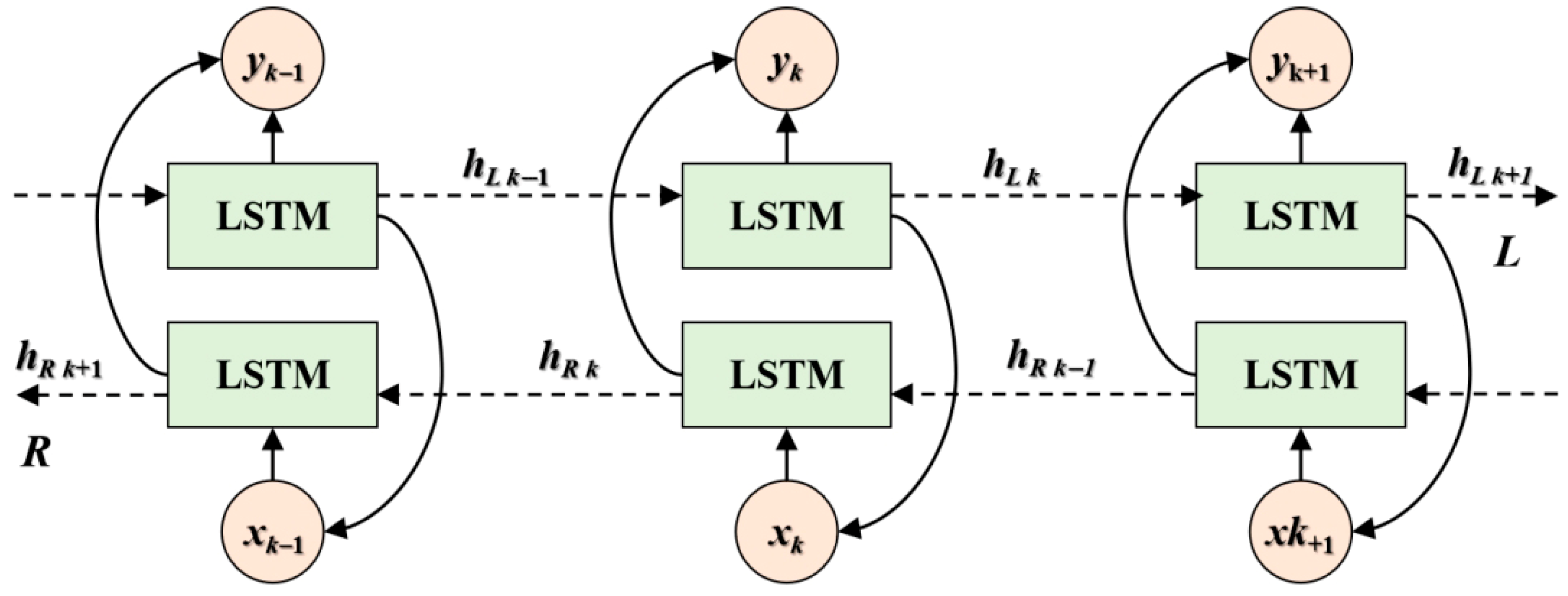
Figure 1. Bi-LSTM structure.
Mathematics 13 02758 g001
Figure 2. Schematic diagram of Bayesian hyperparameter optimization.
Mathematics 13 02758 g002
Figure 3. The proposed prediction and optimization framework.
Mathematics 13 02758 g003
Figure 4. Double-winding method for collecting core loss data.
Mathematics 13 02758 g004
Figure 5. Coefficient fitting results of the SE equation for sinusoidal waveforms: (a) Linear fitting. (b) Nonlinear least square method. (c) Annealing algorithm. (d) Genetic algorithm.
Mathematics 13 02758 g005
Figure 6. Comparison calculation results of the core loss temperature correction model: (a) Linear Correction. (b) Exponential Correction. (c) Logarithmic Correction. (d) Quadratic Correction. (e) Square Root Correction. (f) Multiplicative Correction.
Mathematics 13 02758 g006aMathematics 13 02758 g006b
Figure 7. Kernel density diagram of the calculation results of the core loss temperature correction model: (a) Linear Correction. (b) Exponential Correction. (c) Logarithmic Correction. (d) Quadratic Correction. (e) Square Root Correction. (f) Multiplicative Correction.
Mathematics 13 02758 g007
Figure 8. Square root correction optimization algorithm: (a) Calculation results of core loss. (b) Kernel density plot.
Mathematics 13 02758 g008
Figure 9. Results before and after the correction of the SE equation: (a) Comparison of core losses. (b) Error comparison.
Mathematics 13 02758 g009
Figure 10. Testing results of the core loss prediction model based on Bi-LSTM: (a) Comparison of true values and predicted values. (b) Prediction error of core loss. (c) Core loss prediction value kernel density plot.
Mathematics 13 02758 g010
Figure 11. Performance comparison of Bi-LSTM and three basic machine learning models: (a) Prediction error of core loss. (b) Core loss prediction value kernel density plot.
Mathematics 13 02758 g011
Figure 12. Performance comparison of Bi-LSTM and two basic deep learning models: (a) Prediction error of core loss. (b) Core loss prediction value kernel density plot.
Mathematics 13 02758 g012
Figure 13. Testing results of the core loss prediction model based on Bi-LSTM-Bayes: (a) Comparison of true values and predicted values. (b) Prediction error of core loss.
Mathematics 13 02758 g013
Figure 14. Testing results of the core loss prediction model based on Bi-LSTM-Bayes-ISE: (a) Comparison of true values and predicted values. (b) Prediction error of core loss. (c) Core loss prediction value kernel density plot.
Mathematics 13 02758 g014
Figure 15. Testing results of the core loss prediction model based on Bi-LSTM, Bi-LSTM-Bayes, and Bi-LSTM-Bayes-ISE: (a) Comparison of true values and predicted values. (b) Prediction error of core loss. (c) Core loss prediction value kernel density plot.
Mathematics 13 02758 g015
Figure 16. The Pareto front marginal histogram of core loss and magnetic energy.
Mathematics 13 02758 g016
Figure 17. Optimal solutions based on different decision-making methods.
Mathematics 13 02758 g017
Figure 18. Optimal influencing factors based on different decision-making methods.
Mathematics 13 02758 g018
Figure 19. The Pareto front marginal histogram based on NSGA-II-CSA.
Mathematics 13 02758 g019
Figure 20. Comparison chart of Pareto front before and after the CSA algorithm improvement of the NSGA-II model.
Mathematics 13 02758 g020
Figure 21. Optimal solution charts of NSGA-II-CSA based on different decision-making methods.
Mathematics 13 02758 g021
Figure 22. Optimal influencing factors of NSGA-II-CSA based on different decision-making methods.
Mathematics 13 02758 g022
Table 1. Summary of existing approaches for core loss analysis.
Approach CategoryReferencesVariables ConsideredApplicable ScenariosLimitations
Traditional Physical Models[22,23]Material microstructures, electromagnetic parameters (permeability, coercivity)Fundamental loss mechanism analysisNeglects coupling effects between multiple factors
Classical Empirical Models[31,32]Frequency, flux density amplitudeSinusoidal excitation, isothermal conditionsPoor accuracy under non-sinusoidal waveforms or thermally dynamic environments
Data-Driven Methods[33]Operational parameters (frequency, temperature)PV power forecastingRequires large datasets; limited interpretability
[34]Waveform temporal dependenciesSmall-sample loss predictionComputational complexity for high-dimensional data
[36]Multi-objective loss-heat couplingCore loss optimizationGAN-based methods may suffer from instability in training
[38]Multi-objective lossKolmogorov-Arnold (FS-KAN) networkTime-consuming; Low modeling efficiency
[35]High-frequency HSV driving strategiesEnergy loss minimization in electromagnetic systemsFocus on single-objective optimization; lacks temperature-awareness
Table 2. Statistical values of the dataset in this study.
MaterialsParametersQualitative DataQuantitative Data
MinimumMedianMaximumMeanStandard
Material 1Temperature (°C)25, 50, 70, and 90
Waveformsine, triangle, and trapezoid
Frequency f (Hz) 50,020158,500446,410174,017.8294101,221.4147
Core Loss P (W/m3) 684.046244,323.28443,616,132.5360179,886.9442339,525.6526
Peak Magnetic Flux Density Bm (T) 0.01080.06140.27900.08310.0671
Material 2Temperature (°C)25, 50, 70, and 90
Waveformsine, triangle, and trapezoid
Frequency f (Hz) 49,990158,750501,180210,265.51134,207.3594
Core Loss P (W/m3) 415.613155,545.23642,750,045.7730234,317.1443409,095.6793
Peak Magnetic Flux Density Bm (T) 0.00960.06150.31330.08260.0722
Material 3Temperature (°C)25, 50, 70, and 90
Waveformsine, triangle, and trapezoid
Frequency f (Hz) 49,990158,750501,180212,495.4344135,724.3408
Core Loss (W/m3) 739.334161,055.74013,525,389.2960264,453.0732465,459.5626
Peak Magnetic Flux Density Bm (T) 0.00970.06140.31330.08300.0733
Material 4Temperature (°C)25, 50, 70, and 90
Waveformsine, triangle, and trapezoid
Frequency f (Hz) 50,010125,930446,690170,944.9929110,310.508
Core Loss P (W/m3) 452.227725,284.38442,322,456.1470109,469.2491213,889.8311
Peak Magnetic Flux Density Bm (T) 0.01080.03930.27760.05990.0541
Table 3. Performance of coefficient fitting for sine wave SE equation (unit: W/m3).
Fitting MethodMaxErrorMSERMSEMAER2
Linear fitting283,722.711,791,962,523.4342,331.5719,692.290.9396
Nonlinear least square method240,008.011,616,232,322.9540,202.3920,464.070.9455
Annealing algorithm305,695.372,440,533,358.3249,401.7525,342.420.9177
Genetic algorithm243,344.871,617,941,105.5540,223.6320,651.160.9454
Table 4. Core loss calculation performance of different correction methods (unit: W/m3).
Correction MethodsMaxErrorMSERMSEMAER2
Linear106,838.69264,281,458.9616,256.739564.320.9911
Exponential100,395.71203,849,338.5314,277.588331.750.9931
Logarithmic91,338.985166,977,784.6812,921.987249.310.9944
Quadratic127,806.45607,657,689.7624,650.7114,154.620.9795
Square Root85,248.85136,153,072.04011,668.466776.910.9954
Multiplicative83,406.21185,980,517.4313,637.467629.690.9937
Table 5. Performance of the square root correction optimization algorithm (unit: W/m3).
Algorithm TypeMaxErrorMSERMSEMAER2
Optimization86,582.60134,966,429.9411,617.506736.640.9954
Non-optimized85,248.85136,153,072.04011,668.466776.910.9954
Table 6. Core loss prediction performance based on four basic models.
ModelRMSEMSEMAEMAPESMAPER2
Bi-LSTM70,129.684.92 × 10944,975.22459.1487.810.9023
LSTM85,1067.24 × 10957,879553.3783.2230.8562
GRU76,1155.79 × 10940,982315.9372.6560.8850
SVR2.55 × 1056.53 × 10102.38 × 1053536.6137.05−0.2955
Decision Tree72,4235.25 × 10953,946488.342.450.8859
Linear1.45 × 1052.11 × 10101.13 × 1051885.9121.120.5803
Table 7. Parameter range and optimal hyperparameters for Bayesian hyperparameter optimization.
HyperparameterVariable NameRangeOptimal Hyperparameters
Hidden unitsNumHiddenUnits[20, 100]50
Learning rateLearnRate[1 × 10⁻⁴, 1 × 10⁻²]0.009965
Maximum training numberMaxEpochs[50, 150]56
Batch sizeMiniBatchSize[16, 128]28
Table 8. Core loss prediction performance based on Bayes.
ModelRMSEMSEMAEMAPESMAPER2
Bi-LSTM46,653.232.18 × 10926,622.94165.0463.790.9568
LSTM66,107.284.37 × 10937,681.16193.0374.980.9134
GRU62,423.303.89 × 10935,581.31181.2670.110.9228
SVR120,707.601.46 × 101044,131.70348.29113.560.7112
Decision Tree70,850.725.02 × 10940,384.90201.0273.540.9005
Linear104,403.051.09 × 101068,803.32304.54101.220.7840
Table 9. Core loss prediction performance based on Bi-LSTM-Bayes-ISE.
RMSEMSEMAEMAPESMAPER2
43,615.131.90 × 10926,296.84148.5859.300.9622
Table 10. Hyperparameter settings of the NSGA-II algorithm.
HyperparametersValue
Number of populations200
Number of iterations100
Crossed factors0.8
Variation factors0.25
Table 11. Optimal solutions based on different decision-making methods.
MethodsTemperature (°C)Frequency (Hz)MaterialsWaveformPeak Magnetic Flux Density (T)Core Loss
(W/m3)
Transmit Magnetic Energy (T·Hz)
WSM7085,2442Sinusoidal0.0324522.710.00036
IPM7085,2442Sinusoidal0.0324522.710.00036
EWM7085,2442Sinusoidal0.0324522.710.00036
TOPSIS7085,2442Sinusoidal0.0324522.710.00036
UFM90476,9101Sinusoidal0.07748551,22136,949
RBSM90477,6861Sinusoidal0.10831,201,03051,729
IM90477,1501Sinusoidal0.150312,384,22071,721.1
HOM7085,2442Sinusoidal0.0324522.710.00036
Table 12. Optimal solutions of NSGA-II-CSA based on different decision-making methods.
MethodsTemperature (°C)Frequency (Hz)MaterialsWaveformPeak Magnetic Flux Density (T)Core Loss
(W/m3)
Transmit Magnetic Energy (T·Hz)
WSM70132,0471Sinusoidal0.06287731.5088301.84
IPM70132,0471Sinusoidal0.06287731.5088301.84
EWM70132,0471Sinusoidal0.06287731.5088301.84
TOPSIS70132,0471Sinusoidal0.06287731.5088301.84
UFM90489,6741Sinusoidal0.0841659,55541,201.9
RBSM90491,2831Sinusoidal0.15042,447,99073,888
IM90486,1891Sinusoidal0.14452,259,44070,263.4
HOM70132,0471Sinusoidal0.06287731.5088301.84
Disclaimer/Publisher’s Note: The statements, opinions and data contained in all publications are solely those of the individual author(s) and contributor(s) and not of MDPI and/or the editor(s). MDPI and/or the editor(s) disclaim responsibility for any injury to people or property resulting from any ideas, methods, instructions or products referred to in the content.