High-Precision Dynamic Tracking Control Method Based on Parallel GRU–Transformer Prediction and Nonlinear PD Feedforward Compensation Fusion

Abstract

In high-precision fields such as advanced manufacturing, semiconductor processing, aerospace assembly, and precision machining, motion control systems often face challenges such as large tracking errors and low control efficiency due to complex dynamic environments. To address this, this paper innovatively proposes a data-driven feedforward compensation control strategy based on a Parallel Gated Recurrent Unit (GRU)–Transformer. This method does not require an accurate model of the controlled object but instead uses motion error data and controller output data collected from actual operating conditions to complete network training and real-time prediction, thereby reducing data requirements. The proposed feedforward control strategy consists of three main parts: first, a Parallel GRU–Transformer prediction model is constructed using real-world data collected from high-precision sensors, enabling precise prediction of system motion errors after a single training session; second, a nonlinear PD controller is introduced, using the prediction errors output by the Parallel GRU–Transformer network as input to generate the primary correction force, thereby significantly reducing reliance on the main controller; and finally, the output of the nonlinear PD controller is combined with the output of the main controller to jointly drive the precision motion platform. Verification on a permanent magnet synchronous linear motor motion platform demonstrates that the control strategy integrating Parallel GRU–Transformer feedforward compensation significantly reduces the tracking error and fluctuations under different trajectories while minimizing moving average (MA) and moving standard deviation (MSD), enhancing the system’s robustness against environmental disturbances and effectively alleviating the load on the main controller. The proposed method provides innovative insights and reliable guarantees for the widespread application of precision motion control in industrial and research fields.

1. Introduction

With the continuous development of automated manufacturing and high-precision assembly technologies, precision motion control has been playing an increasingly important role in modern industry [1,2]. In applications such as semiconductor production and micro/nano-manipulation, positioning accuracy at the micrometer or even nanometer level directly impacts product quality and system performance [3,4,5]. However, the increasing complexity of control systems makes many high-performance control algorithms difficult to directly apply to actual equipment. Therefore, developing a control strategy that is structurally simple, easy to implement, and highly performant has become particularly necessary [6,7].

Traditional PID control, including adaptive PID and fuzzy PID, has been widely applied in precision motion platforms due to its simple structure and ease of tuning [8,9,10,11]. However, under conditions such as high-frequency noise, nonlinearity, and time-varying loads, PID control is often susceptible to disturbances [12]. To enhance system robustness, researchers have proposed various robust control methods, such as sliding mode control (SMC), which addresses uncertainties and disturbances by designing a sliding surface, making it suitable for strongly nonlinear systems [13]. However, SMC suffers from chattering issues, which affect system stability and equipment lifespan. Nguyen et al.’s adaptive sliding mode control mitigated chattering to some extent and accelerated system trajectory convergence [14]; H∞ control enhances robustness by minimizing worst-case gains and is widely applied in precision positioning and tracking [15,16]. Jose et al. [17] designed a multivariable controller for a high-precision 6-DOF magnetic levitation positioner and employed a discrete hybrid H2/H∞ filter as the observer. Chen et al. [18] proposed a new observer-based adaptive robust controller (obARC) to address the lack of velocity measurements and compensate for dynamic uncertainties. However, these robust control methods often face limitations such as chattering, sensitivity to modeling errors, and high design complexity. In repetitive tasks, iterative learning control (ILC) and repeated control have demonstrated good trajectory tracking performance [19,20,21]. Zhang et al. proposed an accelerated convergence-based PD-type ILC to improve trajectory tracking for permanent magnet synchronous motors (PMLSMs) [22]. Zheng et al. parallelly integrated adaptive sliding mode control (ASMC) with ILC, achieving both robustness and repeatability in control without an accurate dynamics model [23]. However, in actual engineering applications, repeatedly learning each new trajectory remains time-consuming and labor-intensive.

Besides the above strategies, advanced control methods have also been proposed to enhance robustness, convergence speed, and tracking accuracy under uncertainties. Meng et al. developed an adaptive fixed-time stabilization approach, ensuring convergence within a fixed time and avoiding singularity issues [24]. Lan and Zhao combined Padé approximation-based preview repetitive control with equivalent input disturbance compensation to improve tracking precision and disturbance rejection [25]. Wang et al. introduced a prescribed performance adaptive robust control scheme for robotic manipulators, keeping tracking errors within predefined bounds despite uncertainties [26]. While these approaches have proven effective, the rise of artificial intelligence offers new opportunities to further enhance adaptability and performance in complex, nonlinear, and highly dynamic environments. Feng et al. proposed an adaptive sliding mode control (SMC-RBF) based on radial basis function (RBF) neural networks, effectively compensating for system uncertainties and improving dynamic performance [27]; Hasan et al. designed an adaptive neural network (ANNFOPID) structure combining a nonlinear fractional-order PID controller, utilizing RBF estimation of unknown disturbances to enhance the robustness of the control system [28]; Yang et al. proposed an adaptive dual-neural network sliding mode control (ADNSMC) by integrating recurrent neural networks (RNNs) with RBF neural networks and combining them with non-singular fast terminal sliding mode control (NFTSMC) to improve accuracy and convergence speed [29]; Hu et al. utilized neural networks for feedforward compensation to achieve pre-correction of tracking errors [30,31,32]; and Zhou proposed an intelligent gated recurrent unit (GRU) real-time iterative compensation (RIC) position-loop feedforward compensation control method, balancing offline compensation and real-time iterative compensation, effectively reducing residual error [33]. However, these neural network methods often face challenges such as high computational complexity and insufficient real-time performance in high-speed, high-dynamic environments, especially in embedded systems or resource-constrained scenarios, where latency and computational overhead can easily lead to degraded control performance.

This paper proposes a novel data-driven feedforward compensation control strategy that utilizes a Parallel GRU–Transformer network for efficient prediction of motion errors in precision motion control systems. Compared to traditional prediction methods based on single GRU or Transformer models, the proposed Parallel GRU–Transformer network combines the local sequence feature capture capability of a GRU with the global dependency modeling advantage of a Transformer [34], enabling accurate and efficient prediction of the next moment’s motion error using two types of simplified input data: motion error and controller output. Subsequently, by feeding the prediction error into a nonlinear PD controller [35] to generate a feedforward compensation signal and driving the motion platform together with the main controller’s output, the system completes the compensation action before the actual error occurs, significantly reducing the amplitude of the motion error. This method effectively alleviates the real-time adjustment burden of the feedback controller and further improves the response speed and accuracy of the control system by adapting to the inherent nonlinear characteristics of the system through the nonlinear PD controller. Additionally, the proposed feedforward compensation scheme demonstrates significant versatility and convenience, enabling seamless integration with existing controller architectures. Experimental validation on a permanent magnet synchronous linear motor motion platform confirms that the method effectively reduces system tracking error and variability metrics, such as MA (moving average) and MSD (moving standard deviation), under various operating conditions, thereby enhancing the system’s robustness against external disturbances and control stability.

The main contributions of this paper are as follows:

(1) A Parallel GRU–Transformer prediction model is proposed. By reasonably constructing the training dataset, the model can accurately model the temporal dynamic characteristics of the system without requiring an accurate model of the controlled object. It only uses the motion error and controller output under actual operating conditions as network inputs, requires a small amount of data, and can effectively predict the motion error at future time instants.

(2) An efficient feedforward compensation control strategy based on a nonlinear PD controller is designed. The proposed method can be directly deployed in actual engineering systems and can be efficiently integrated with existing control strategies, significantly simplifying the implementation difficulty in actual industrial sites.

(3) Through experiments conducted on a permanent magnet synchronous linear motor motion platform under different operating conditions, the effectiveness and robustness of the proposed control method under actual operating conditions are verified, demonstrating its excellent industrial practical value.

The structure of this paper is as follows: Section 1 models and analyzes the system and introduces the main characteristics of the motion platform. Section 2 discusses the feedforward compensation control strategy based on the Parallel GRU–Transformer neural network prediction, detailing the network structure, training process, feedforward compensation method, and system stability analysis. Section 3 verifies the prediction effect through comparative experiments and the performance of the proposed control strategy under different operating conditions. Finally, Section 4 summarizes the research results.

2. System Modeling

The PMLSM is a highly coupled, multivariable, and intricate nonlinear system necessitating decoupling analysis. In the $\alpha$-$\beta$ stationary coordinate system, the voltage equation of the stator’s two-phase winding is articulated as in (1).

$$\left[\begin{array}{c}{u}_{\alpha }\\ u_{\beta }\end{array}\right]=\left[\begin{array}{cc}R+\rho L_d& -{\omega }_e(L_d-L_q)\\ {\omega }_e(L_d-L_q)& R+\rho L_d\end{array}\right]\left[\begin{array}{c}{i}_{\alpha }\\ i_{\beta }\end{array}\right]+\left[\begin{array}{c}{e}_{\alpha }\\ e_{\beta }\end{array}\right]$$

(1)

Here, $u_{\alpha }$ and $u_{\beta }$ are the stator voltages in the $\alpha$-$\beta$ coordinate system and $i_{\alpha }$ and $i_{\beta }$ are the stator currents in the $\alpha$-$\beta$ coordinate system; R is the phase resistance; $L_d$ and $L_q$ are the stator inductance; $\rho =d/dt$ represents the differential operator; ${\omega }_e$ is the angular velocity; and $e_{\alpha }$ and $e_{\beta }$ are the extended back electromotive force, expressed as in (2).

$$\left[\begin{array}{c}{e}_{\alpha }\\ e_{\beta }\end{array}\right]=\left[(L_d-L_q)\left({\omega }_e{i}_d-{\displaystyle \frac{d{i}_q}{dt}}\right)+{\omega }_e{\psi }_f\right]\left[\begin{array}{c}-sin\theta \\ cos\theta \end{array}\right]$$

(2)

The extended back electromotive force contains positional information, from which the rotor electrical angular velocity ${\omega }_e$ and electrical angle ${\theta }_e$ can be extracted, represented as (3).

$$\left\{\begin{array}{cc}\hfill {\theta }_e& =-arctan{\displaystyle \frac{e_{\alpha }}{e_{\beta }}}\hfill \\ \hfill {\omega }_e& ={\displaystyle \frac{d{\theta }_e}{dt}}\hfill \end{array}\right.$$

(3)

For ease of control, the $\alpha$-$\beta$ coordinate system is often transformed through rotation to the rotor synchronous rotation coordinate system (d-q coordinates). The mathematical model in d-q rotating coordinates is represented as in (4).

$$\rho \left[\begin{array}{c}{L}_d{i}_d\\ -L_q{i}_q\end{array}\right]=\left[\begin{array}{c}{u}_d\\ u_q\end{array}\right]-R\left[\begin{array}{c}{i}_d\\ i_q\end{array}\right]+{\omega }_e\left[\begin{array}{c}{L}_q{i}_q\\ -L_d{i}_d\end{array}\right]-\left[\begin{array}{c}{E}_d\\ E_q\end{array}\right]$$

(4)

Here, $u_d$ and $u_q$ are the stator voltages on the d- and q-axes, $i_d$ and $i_q$ are the stator currents on the d- and q-axes, and $E_d$ and $E_q$ are the induced electromotive forces on the d- and q-axes. When selecting an appropriate coordinate system such that the magnetic flux ${\psi }_f$ of the permanent magnet is completely on the d-axis, $E_d$ can be set to 0, $E_q={\omega }_e{\psi }_f$. $E_q$ contains speed information, and the position information of the rotor can be obtained by integrating the speed ${\omega }_e$, represented as (5).

$$\left\{\begin{array}{cc}\hfill {\omega }_e& ={\displaystyle \frac{E_q}{{\psi }_f}}\hfill \\ \hfill {\theta }_e& =\int {\omega }_{e}dt\hfill \end{array}\right.$$

(5)

The electromagnetic torque and mechanical motion equation of the motor are expressed as (6) and (7).

$$T_e={\displaystyle \frac{3}{2}}{p}_n{i}_q[i_d(L_d-L_q)+{\psi }_f]$$

(6)

$$J{\displaystyle \frac{d{\omega }_m}{dt}}=T_e-T_L-B{\omega }_m$$

(7)

where $p_n$ is the number of motor poles, ${\psi }_f$ is the stator permanent magnet flux, ${\omega }_m=p_n/{\omega }_e$ is the mechanical angular velocity of the motor, $T_e$ is the electromagnetic torque, $T_L$ is the load torque, B is the viscous resistance coefficient, and J is the rotor moment of inertia.

The above model can achieve an accurate description of the electromagnetic and motion characteristics of the PMLSM, laying a theoretical foundation for subsequent control system design. The next section will introduce the detailed design process of the control architecture.

2.1. Control Architecture Based on Parallel GRU–Transformer Feedforward Compensation

2.1.1. Structure of Parallel GRU–Transformer

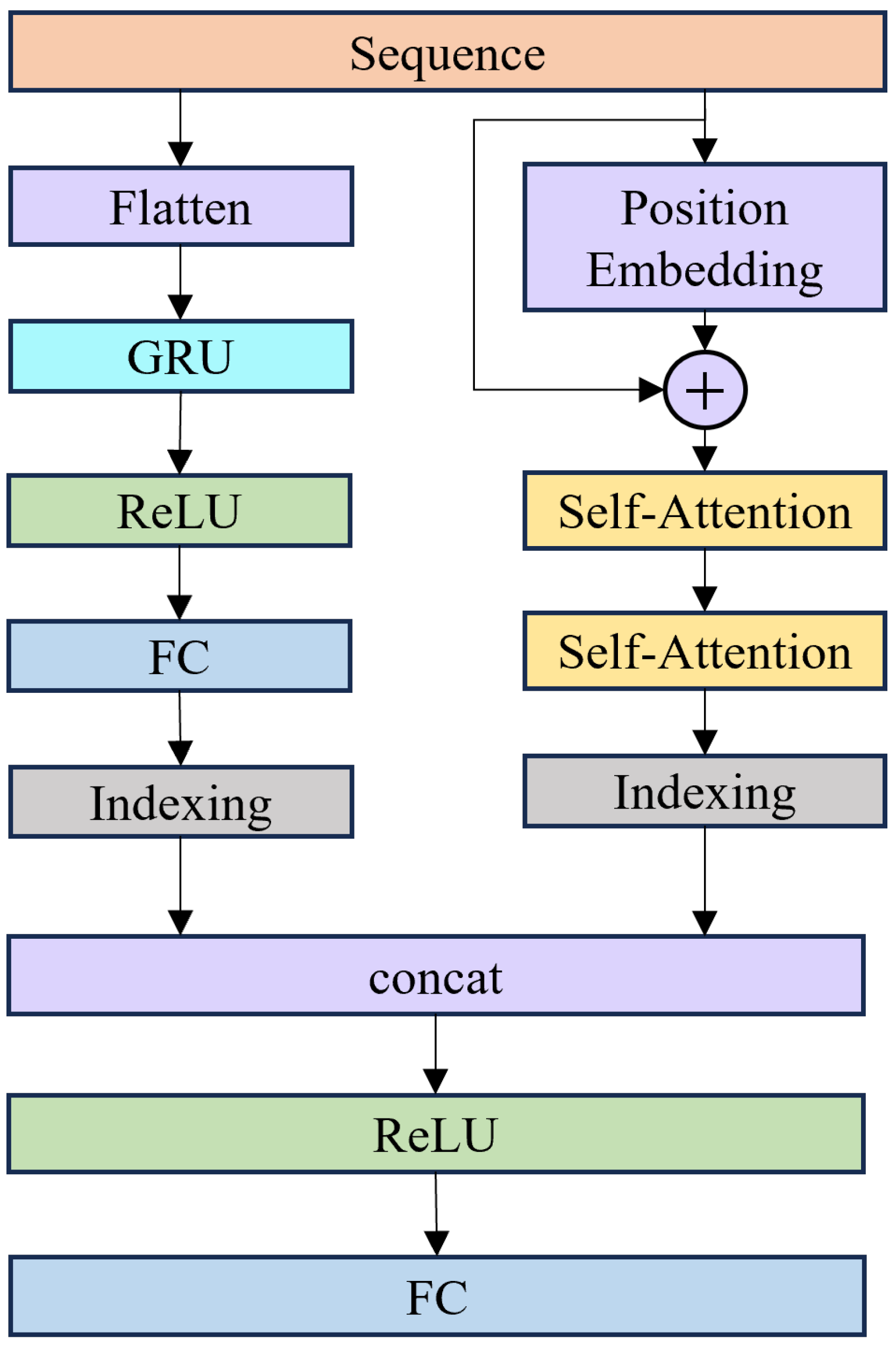
This paper proposes a Parallel GRU–Transformer neural network architecture that aims to combine the advantages of gated recurrent units (GRUs) and Transformers to simultaneously capture local dynamics and global dependencies in time series. As shown in Figure 1, the architecture consists of two parallel branches, namely the GRU branch and the Transformer branch, which extract complementary features through different mechanisms.

A GRU is an improved version of the Long Short-Term Memory (LSTM) network [36], simplifying the gating mechanism to enhance training efficiency while retaining strong sequence modeling capabilities. The GRU structure only includes an update gate and a reset gate, omitting explicit memory units. The update gate controls the extent to which information from the previous hidden state is retained in the current state, as shown in (8).

$$z_t=\sigma \left(W_z[h_{t-1},x_t]\right)$$

(8)

In this equation, $\sigma (·)$ is the sigmoid activation function, $W_z$ is the learnable weight matrix, $[h_{t-1},x_t]$ denotes the concatenation of the previous hidden state and the current input, and the reset gate is used to control the degree of selective forgetting of the previous hidden state, as shown in (9).

$$r_t=\sigma \left(W_r[h_{t-1},x_t]\right)$$

(9)

Under reset door control, the candidate hidden state can be represented as (10).

$${\tilde{h}}_t=tanh\left(W[r_t\odot h_{t-1},x_t]\right)$$

(10)

Here, ⊙ denotes element-wise multiplication and $tanh(·)$ is the hyperbolic tangent activation function. The final hidden state is obtained by weighting and fusing the historical states and candidate states through the update gate, as shown in (11).

$$h_t=(1-z_t)\odot h_{t-1}+z_t\odot {\tilde{h}}_t$$

(11)

The Transformer architecture is based on a self-attention mechanism, which explicitly introduces sequence position information through position encoding to capture long-range dependencies. The position encoding calculation methods are shown in (12) and (13).

$$PE(pos,2i)=sin\left({\displaystyle \frac{pos}{{10000}^{2i/d_{model}}}}\right)$$

(12)

$$PE(pos,2i+1)=cos\left({\displaystyle \frac{pos}{{10000}^{2i/d_{model}}}}\right)$$

(13)

In this context, $pos$ denotes the sequence position, i denotes the index of the encoding dimension, and $d_{model}$ denotes the feature dimension of the model. The input feature matrix X undergoes linear mapping to obtain the query Q, key K, and value V, which are represented as (14)–(16).

$$Q=X{W}^Q$$

(14)

$$K=X{W}^K$$

(15)

$$V=X{W}^V$$

(16)

Here, $W^Q$, $W^K$, and $W^V$ are the corresponding weight matrices. Then, the attention output is obtained using the scaled point-wise attention mechanism, expressed as in (17).

$$Attention(Q,K,V)=\mathrm{softmax}\left({\displaystyle \frac{Q{K}^T}{\sqrt{d_k}}}\right)V$$

(17)

In the equation, $1/\sqrt{d_k}$ is the scaling factor to prevent the dot product from becoming too large, which would cause the gradient to disappear. To further improve the model’s expressive power, the Transformer uses a multi-head attention mechanism to divide the input into multiple subspaces, calculate the attention separately, and then concatenate them to form (18).

$$MultiHead(Q,K,V)=\mathrm{Concat}(hea{d}_1,\dots ,hea{d}_h)W^O$$

(18)

Here, the calculation formula for the i-th head is expressed as (19).

$$hea{d}_i=Attention(Q{W}_i^Q,K{W}_i^K,V{W}_i^V)$$

(19)

$W_i^Q$, $W_i^K$, and $W_i^V$ are the projection matrices of the i-th head and $W^O$ is the output mapping matrix, which maps the multi-head attention outputs back to the original model feature space.

In the Parallel GRU–Transformer architecture, the input sequence is fed into two branches, GRU and Transformer, for parallel processing. In the GRU branch, the input sequence is flattened and then enters a GRU layer containing 10 units, followed by a ReLU activation function and a fully connected layer. A specific indexing layer extracts the features at the last moment of the sequence to capture local dynamic information. The Transformer branch fuses the original sequence features through position encoding and uses two self-attention layers (each with four attention heads and 64-dimensional key channels) to capture global dependency features in the sequence. Finally, an indexing layer extracts the feature representations at the end of the sequence.

The features from both branches are then concatenated and fused, and through ReLU activation and fully connected mapping to the target output space, the final prediction results are generated. This parallel structure effectively overcomes the shortcomings of a single GRU in capturing long-range dependencies, while also addressing the limitations of Transformers in perceiving fine-grained local dynamics, providing a complex time series prediction method that is both efficient and robust.

2.1.2. Nonlinear PD Controller

Traditional linear PD control often struggles to balance fine control in small-error regions with fast convergence in large-error regions when dealing with systems with large-scale variations and strong disturbances. Therefore, a PD control form based on nonlinear gain scheduling has been proposed in the literature, whose core idea is to introduce a nonlinear function $\mathrm{fal}(·)$ to the error and its derivative and to characterize the gain requirements of different error intervals in a segmented or nonlinear manner. This is expressed as (20).

$$u={\beta }_1\mathrm{fal}(e_1,{\alpha }_1,\delta )+{\beta }_2\mathrm{fal}(e_2,{\alpha }_2,\delta )$$

(20)

where $e_1$ and $e_2$, respectively, represent the position error and the differentiated position error, ${\beta }_1$ and ${\beta }_2$ are the gain coefficients, and ${\alpha }_1$, ${\alpha }_2$, and $\delta$ determine the shape and threshold of the segmented nonlinearity. The function $\mathrm{fal}(·)$ is represented as (21).

$$\mathrm{fal}(e,\alpha ,\delta )=\left\{\begin{array}{cc}{\displaystyle \frac{e}{{\delta }^{1-\alpha }}},\hfill & \left|e\right|\le \delta \hfill \\ {\left|e\right|}^{\alpha }\mathrm{sign}\left(e\right),\hfill & \left|e\right|>\delta \hfill \end{array}\right.$$

(21)

The nonlinear PD controller adjusts its effective gain according to the magnitude of the tracking error. In the small-error region ($\left|e\right|\le \delta$), the gain is proportionally reduced to limit overshoot and improve noise tolerance. In the large-error region ($\left|e\right|>\delta$), the gain is increased following a nonlinear power law, enabling rapid suppression of large deviations. Parameters ${\alpha }_1$ and ${\alpha }_2$ determine the degree of nonlinearity: smaller values provide smoother control near the origin, while values closer to 1 improve responsiveness for large errors. Gains ${\beta }_1$ and ${\beta }_2$ balance the contributions from position and velocity feedback, and $\delta$ defines the boundary between the small- and large-error regions, chosen based on sensor resolution and noise level. Compared with a conventional PD controller with fixed gains, the nonlinear PD applies a higher gain only when necessary, achieving faster recovery from large disturbances while maintaining stability and high accuracy near the target.

2.1.3. Tracking Error Prediction Based on Parallel GRU–Transformer Neural Network

This study collected a high-quality dataset of 100 s of data on a high-precision motion platform driven by a permanent magnet synchronous motor for training a Parallel GRU–Transformer network. The platform is equipped with a $0.5\mathsf{\mu }$m resolution optical grating displacement sensor, and the output signal is decoded orthogonally by a $10\mathrm{MHz}$ sampling FPGA board to obtain high-precision real-time displacement information. 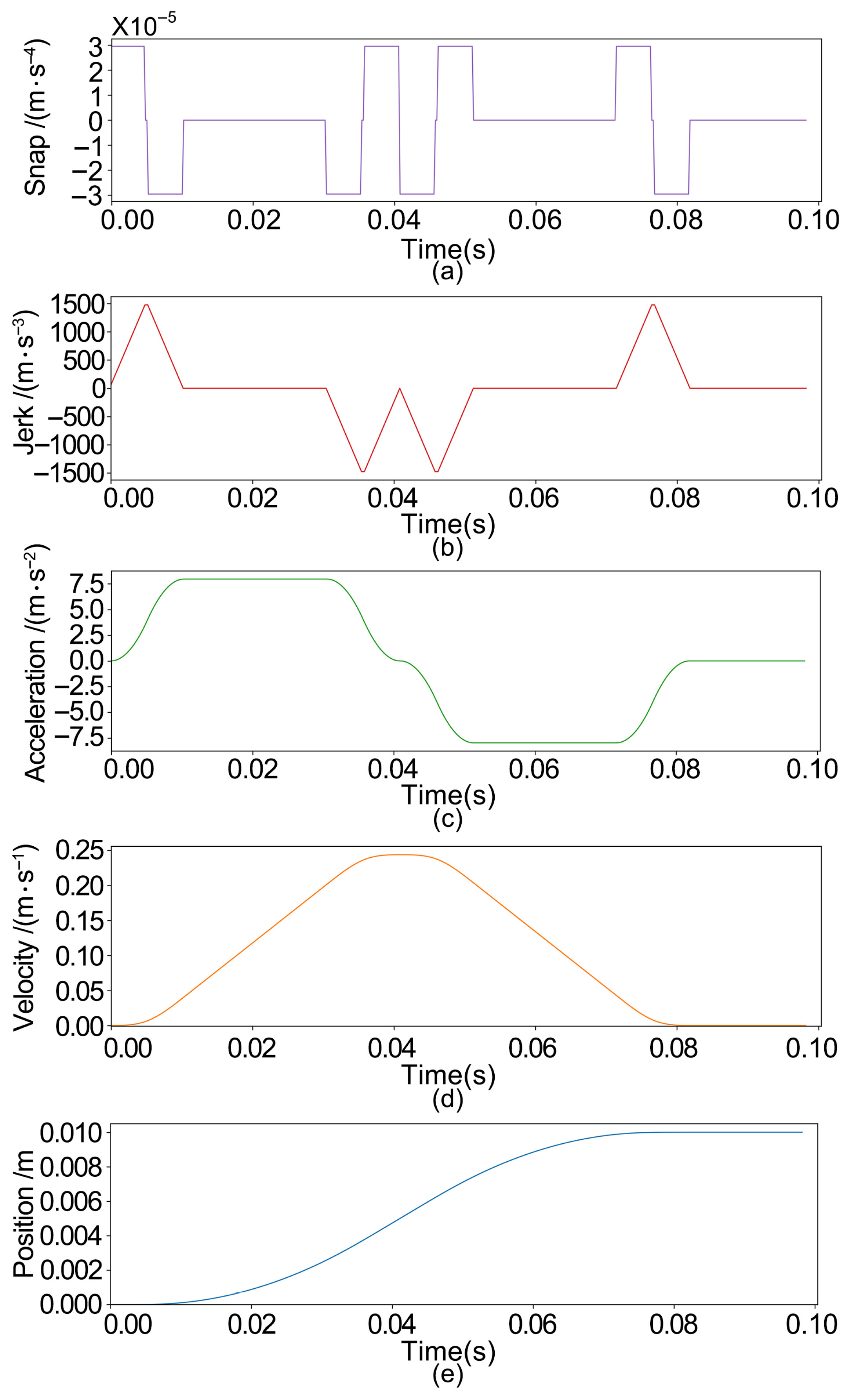The main controller collects the actual position at a frequency of $5\mathrm{kHz}$, compares it with the fourth-order polynomial reference trajectory point by point, calculates the tracking error, and generates the controller output through a feedback loop. The complete trajectory is composed of multiple segments of fourth-order polynomials, as shown in Figure 2. The load is kept constant during the experiment.

All raw data are first normalized to [−1, 1] using Min–Max normalization after acquisition to ensure that all variables are uniformly distributed within similar numerical intervals, thereby improving the convergence speed and stability of network training. After normalization, the tracking error sequence $\mathbf{e}$ and the corresponding control output sequence $\mathbf{u}$ for the first N time steps are combined in time order to form a complete input matrix $\mathbf{X}$, which is used as the input for the Parallel GRU–Transformer training set. The $\mathbf{u}$ at time step N+1 is used as the output. Its format is defined as (22) and (23).

$$\mathbf{e}={[e_1,e_2,\dots ,e_N]}^T$$

(22)

$$\mathbf{u}={[u_1,u_2,\dots ,u_N]}^T$$

(23)

where $e_i$ denotes the tracking error at the ith ($i=1,2,\dots ,N$) discrete time step, whereas $u_i$ signifies the controller output at the same time step, together encapsulating the dynamic evolution of the system during the historical phase. Combine the error $\mathbf{e}$ over N time steps and the controller output $\mathbf{u}$ into a matrix $\mathbf{X}$ with dimensions $N\times 2$. The comprehensive input data matrix $\mathbf{X}$ can be derived in the following precise format (24).

$$\mathbf{X}=\left[\begin{array}{cc}{e}_1& u_1\\ e_2& u_2\\ ⋮& ⋮\\ e_N& u_N\end{array}\right]$$

(24)

After multiple experiments, the window length N was determined to be 10. Finally, the normalized data was divided into training and validation sets in a ratio of 8:2 to comprehensively evaluate the performance of the Parallel GRU–Transformer in error prediction and feedforward compensation.

2.1.4. Parallel GRU–Transformer-Based Feedforward Compensation Framework

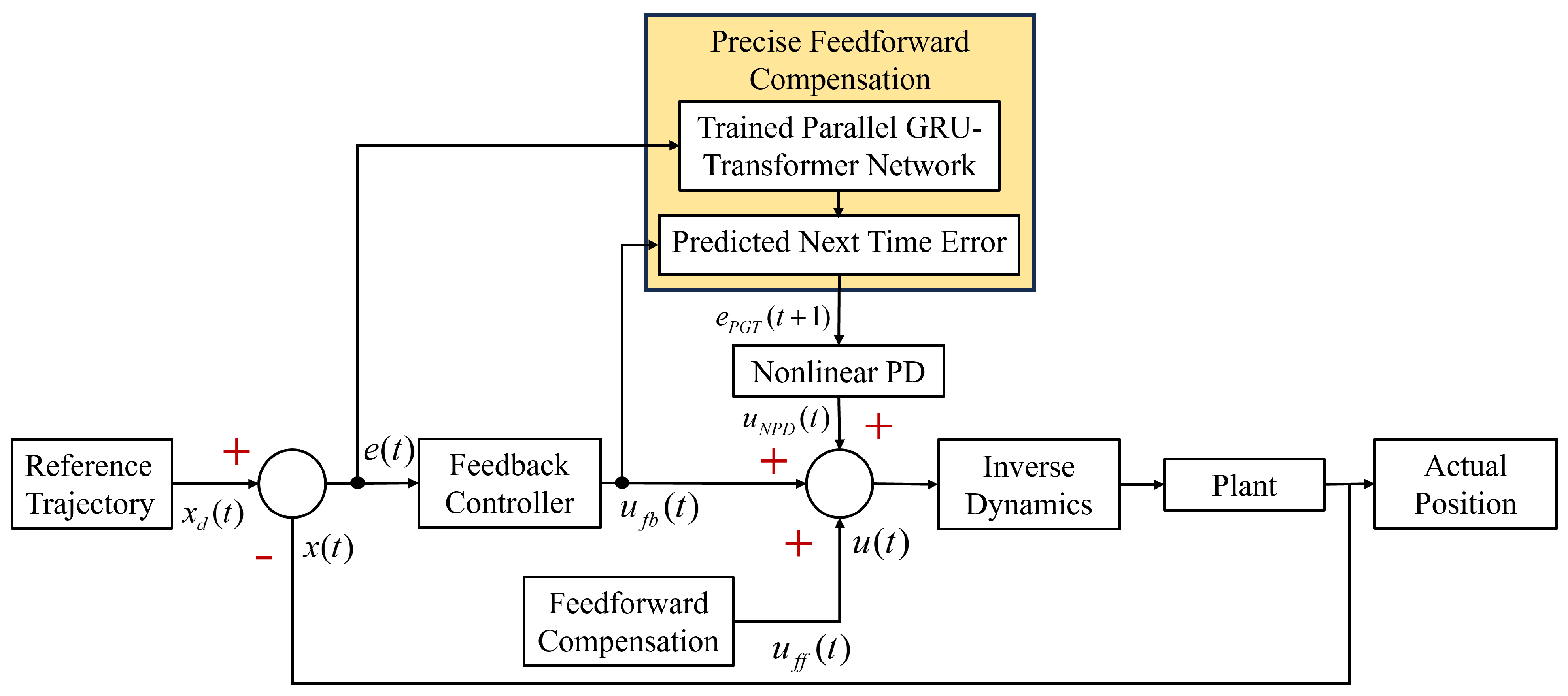
This section gives the servo control architecture of the PMLSM motion platform, as shown in Figure 3. The total control input of the system consists of the following three parts, expressed as (25).

$$u\left(t\right)=u_{fb}\left(t\right)+u_{ff}\left(t\right)+u_{NPD}\left(t\right)$$

(25)

where $u_{fb}\left(t\right)$ is the feedback controller output, $u_{ff}\left(t\right)$ is the feedforward compensation output, and $u_{NPD}\left(t\right)$ is the control quantity of the next time error predicted based on the Parallel GRU–Transformer network and corrected by the nonlinear PD module. $u\left(t\right)$ acts on the plant, and the output is the actual position $x\left(t\right)$. The error signal $e\left(t\right)$ of the system is defined by the difference between the reference trajectory $x_d\left(t\right)$ and the actual output $x\left(t\right)$ as in (26).

$$e\left(t\right)=x_d\left(t\right)-x\left(t\right)$$

(26)

The feedback controller adopts a PID controller, whose output is expressed as (27).

$$u_{fb}\left(t\right)=K_{p}e\left(t\right)+K_i{\int }_0^{t}e\left(\tau \right)d\tau +K_d{\displaystyle \frac{de\left(t\right)}{dt}}$$

(27)

Feedforward compensation consists of acceleration and velocity feedforward terms, expressed as (28).

$$u_{ff}\left(t\right)=K_a{x}_a\left(t\right)+K_v{x}_v\left(t\right)$$

(28)

where $x_a\left(t\right)$ is the acceleration trajectory, $x_v\left(t\right)$ is the velocity trajectory, and $K_a$ and $K_v$ are the acceleration and velocity feedforward gains, respectively, used to quickly compensate for the dynamic changes in high-order motion. The nonlinear PD controller receives the next time error output predicted by the Parallel GRU–Transformer network and performs nonlinear correction on it. The Parallel GRU–Transformer network takes $e\left(t\right)$ and $u_{fb}\left(t\right)$ as inputs and generates a prediction error, expressed as (29).

$$e_{PGT}(t+1)=f_{PGT}(e\left(t\right),u_{fb}\left(t\right))$$

(29)

where $e_{PGT}(t+1)$ represents the next time position error predicted by the Parallel GRU–Transformer network. Based on this, the output of the nonlinear PD controller is expressed as (30).

$$u_{NPD}\left(t\right)={\beta }_1\mathrm{fal}(e_{PGT}(t+1),{\alpha }_1,\delta )+{\beta }_2\mathrm{fal}\left({\displaystyle \frac{d{e}_{PGT}(t+1)}{dt}},{\alpha }_2,\delta \right)$$

(30)

The total system control input $u\left(t\right)$ combines $u_{NPD}\left(t\right)$, $u_{ff}\left(t\right)$, and $u_{fb}\left(t\right)$ to act on the controlled object to ensure the stability and accuracy of the system when dealing with complex dynamic characteristics. The results of the prediction and tracking error will be shown in the next chapter.

2.1.5. Stability Analysis

According to the previous subsection, the linearized error dynamics equation is expressed as (31).

$${\displaystyle \frac{de\left(t\right)}{dt}}=Ae\left(t\right)+B{u}_{fb}\left(t\right)$$

(31)

where A and B are the state matrix and input matrix of the system (linearized near the equilibrium point). Define the candidate Lyapunov function as (32).

$$V_1\left(t\right)={\displaystyle \frac{1}{2}}{e}^2\left(t\right)+{\displaystyle \frac{1}{2}}\gamma {\left({\int }_0^{t}e\left(\tau \right)d\tau \right)}^2,\gamma >0$$

(32)

When and only when $e\left(t\right)=0$, ${\int }_0^{t}e\left(\tau \right)d\tau =0$ and $V_1\left(t\right)=0$. For any non-zero state, $V_1\left(t\right)>0$ is obvious, so $V_1\left(t\right)$ satisfies the positive definiteness condition of the Lyapunov function. Differentiating $V_1\left(t\right)$ yields (33).

$${\dot{V}}_1\left(t\right)=e\left(t\right)\dot{e}\left(t\right)+\gamma \left({\int }_0^{t}e\left(\tau \right)d\tau \right)·e\left(t\right)$$

(33)

Substituting into the system error dynamics equation yields (34).

$$\begin{array}{cc}\hfill {\dot{V}}_1\left(t\right)& =e\left(t\right)\left[Ae\left(t\right)+B\left(K_{p}e\left(t\right)+K_i{\int }_0^{t}e\left(\tau \right)d\tau +K_d\dot{e}\left(t\right)\right)\right]+\gamma \left({\int }_0^{t}e\left(\tau \right)d\tau \right)e\left(t\right)\hfill \\ \hfill & =e\left(t\right)\left[Ae\left(t\right)+B\left(K_{p}e\left(t\right)+K_i{\int }_0^{t}e\left(\tau \right)d\tau +K_{d}Ae\left(t\right)\right)\right]+\gamma \left({\int }_0^{t}e\left(\tau \right)d\tau \right)e\left(t\right)\hfill \\ \hfill & =e\left(t\right)\left[\left(A+B{K}_p+B{K}_{d}A\right)e\left(t\right)+B{K}_i{\int }_0^{t}e\left(\tau \right)d\tau \right]+\gamma \left({\int }_0^{t}e\left(\tau \right)d\tau \right)e\left(t\right)\hfill \end{array}$$

(34)

Here, $\dot{e}\left(t\right)$ is approximated by $Ae\left(t\right)$ from (31), neglecting higher-order nonlinear terms near the equilibrium point for analytical tractability. Let the state vector be (35).

$$X\left(t\right)=\left[\begin{array}{c}e\left(t\right)\\ z\left(t\right)\end{array}\right],z\left(t\right)={\int }_0^{t}e\left(\tau \right)d\tau$$

(35)

Therefore, ${\dot{V}}_1\left(t\right)$ is expressed as (36).

$${\dot{V}}_1\left(t\right)=X^{\top }\left(t\right)QX\left(t\right),Q\triangleq \left[\begin{array}{cc}A+B{K}_p+B{K}_{d}A& {\displaystyle \frac{1}{2}}(B{K}_i+\gamma )\\ {\displaystyle \frac{1}{2}}(B{K}_i+\gamma )& 0\end{array}\right]$$

(36)

By appropriately choosing $K_p$, $K_i$, $K_d$, and $\gamma$, the symmetric matrix Q can be made negative definite, which yields the existence of $\lambda >0$ such that (37) holds.

$${\dot{V}}_1\left(t\right)\le -\lambda e^2\left(t\right),\lambda >0$$

(37)

This guarantees exponential convergence of the tracking error. Although this is not strict finite-time convergence, it provides sufficiently fast decay in practice to meet the application requirements. Here, $\lambda$ represents the lower bound of the convergence rate; a larger $\lambda$ results in faster error decay. The matrix Q is expressed as (38).

$$Q=\left[\begin{array}{cc}A+B{K}_p+B{K}_{d}A& {\displaystyle \frac{1}{2}}\left(B{K}_i+\gamma \right)\\ {\displaystyle \frac{1}{2}}\left(B{K}_i+\gamma \right)& 0\end{array}\right]$$

(38)

The $\mathrm{fal}(·)$ function in the previous subsection has global Lipschitz continuity, so it satisfies global boundedness; i.e., there exists a normal number $M_f$ that satisfies (39).

$$\left|\mathrm{fal}(e,\alpha ,\delta )\right|\le M_f\left(\left|e\right|+{\left|e\right|}^{\alpha }\right),\forall e\in \mathbb{R}$$

(39)

Based on the training process of the Parallel GRU–Transformer network, the neural network outputs a one-step-ahead position error prediction, denoted by ${\tilde{e}}_p\left(t\right)$ (aligned to time t). The nonlinear PD compensator uses ${\tilde{e}}_p\left(t\right)$ and its discrete-time derivative, as given in (40).

$$d_p\left(t\right)\triangleq {\displaystyle \frac{{\tilde{e}}_p\left(t\right)-{\tilde{e}}_p(t-\mathsf{\Delta })}{\mathsf{\Delta }}}$$

(40)

where $\mathsf{\Delta }$ is the sampling interval. Since the network is trained on bounded trajectories and operates within the plant’s physical limits, it is reasonable to assume the boundedness for some positive constants $M_p,M_d$, as given in (41).

$$|{\tilde{e}}_p\left(t\right)|\le M_p,\left|d_p\left(t\right)\right|\le M_d,\forall t\ge 0$$

(41)

With a globally Lipschitz $fal(·)$ nonlinearity (previous subsection), the nonlinear PD input satisfies (42).

$$|u_{PD}\left(t\right)|\le {\beta }_1{M}_f\left(|{\tilde{e}}_p\left(t\right)|+|{\tilde{e}}_p{\left(t\right)|}^{{\alpha }_1}\right)+{\beta }_2{M}_f\left(|d_p\left(t\right)|+|d_p{\left(t\right)|}^{{\alpha }_2}\right)\le M_u,$$

(42)

where ${\alpha }_1,{\alpha }_2\in (0,1]$ and $M_u$ is a positive constant determined by $(M_p,M_d,{\beta }_1,{\beta }_2,M_f)$. Therefore, under the globally Lipschitz $fal(·)$ nonlinearity, the nonlinear PD compensation control law yields a globally bounded input, which can be regarded as a bounded disturbance to the closed-loop system.

Considering the closed-loop system error state $e\left(t\right)$, the overall closed-loop dynamics can be expressed as (43).

$$\dot{e}\left(t\right)=f\left(e\left(t\right)\right)+g\left(e\left(t\right)\right)u_{PD}\left(t\right)$$

(43)

Since the system is locally asymptotically stable when there is no disturbance ($u_{PD}\left(t\right)=0$), there exists an Input-to-State Stability (ISS)-type Lyapunov function $V_{ISS}\left(e\right)$ satisfying (44).

$${\dot{V}}_{ISS}\left(e\right)\le -\alpha (\parallel e\parallel )+\gamma (\parallel u_{PD}\left(t\right)\parallel )$$

(44)

where $\alpha (·)$ is a ${\mathcal{K}}_{\infty }$ class function and $\gamma (·)$ is a $\mathcal{K}$ class function. If the controller parameters are chosen appropriately, the closed-loop system gain is sufficiently small to satisfy the small gain condition; i.e., there exists a constant $\sigma \in (0,1)$ satisfying (45).

$$\gamma \left(M_u\right)\le \sigma \alpha (\parallel e\parallel )$$

(45)

Then, according to the small gain theorem, the overall system is ISS-stable.

3. Experimental Investigation

3.1. Experimental Setup

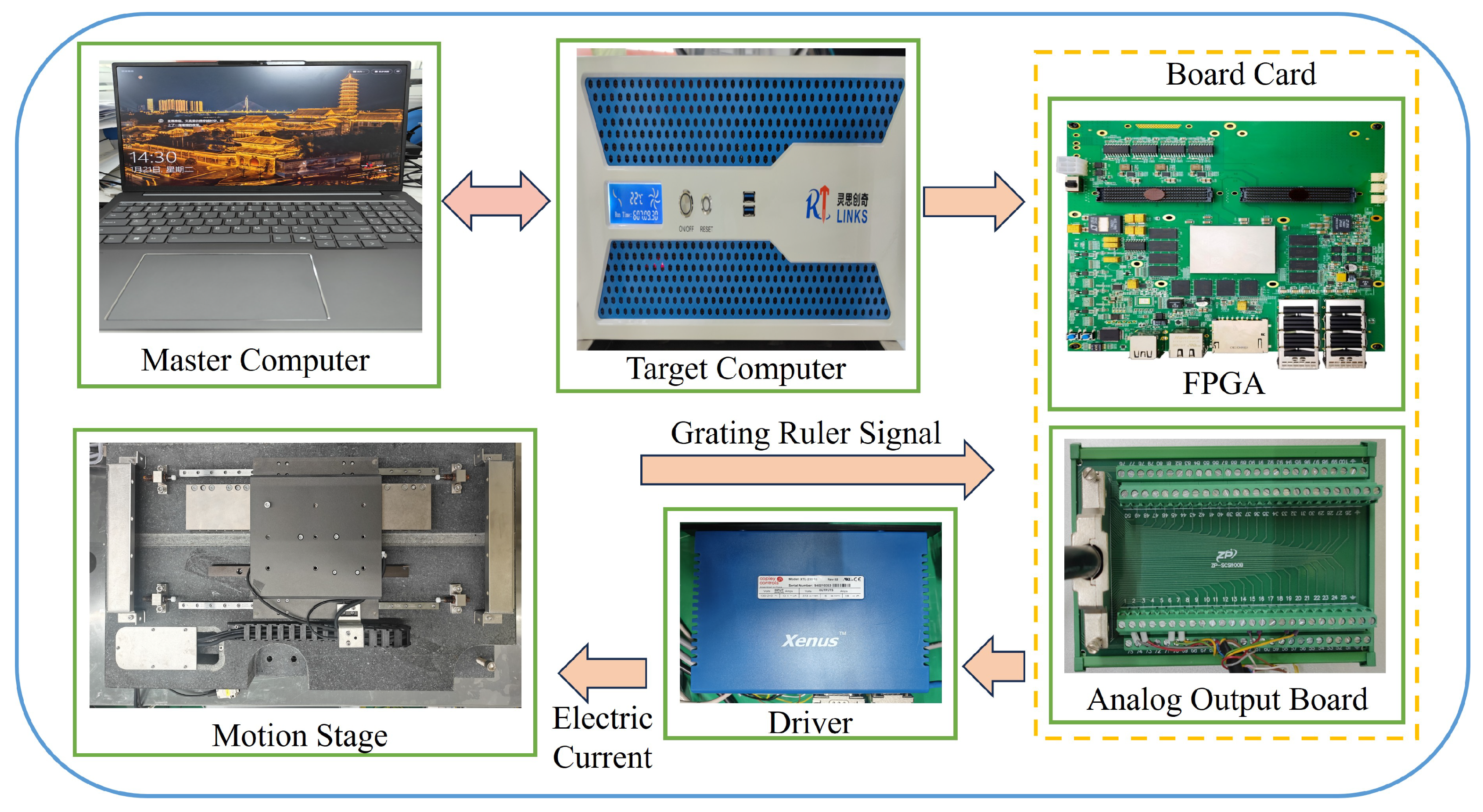
An experimental platform was constructed to validate the real-time performance and predictive accuracy of the proposed method, incorporating essential modules, including an upper computer, a real-time simulator, an FPGA board, an analog output board, a driver, and a motion platform, as depicted in Figure 4. Bidirectional exchange of high-speed data and instructions between the host computer and the real-time simulator is facilitated via the IP protocol. The real-time simulator performs the primary functions of real-time control and algorithmic computation in this process: it implements control strategies derived from the gathered sensor data, turns control signals into current via the analog output board, and transmits it to the driver. The driver accurately maneuvers the motion platform using current regulation. A high-precision grating ruler serves as a position sensor on the motion platform, with its output signal being gathered and preprocessed by an FPGA board before being relayed to the real-time simulator, therefore establishing a closed-loop control system. The system incorporates high-bandwidth, low-latency communication techniques and real-time data processing capabilities, guaranteeing the precision and immediacy of motion control, while also offering robust experimental validation for the reliability and efficacy of the proposed predictive model. The hardware specifications are presented in

Table 1. Experimental configuration.

Hardware	Parameter
Real-time simulation machine	CPU: Intel Core i9-9900KS@4.00 GHz octa-core; 8 GB DDR3 SDRAM; operating system: RTOS
Analog output board	D/A conversion accuracy: 16-bit; voltage output: 16-channel; output range: +/−10 V; conversion rate: 25 V/us; set up time: 2 us
FPGA board	CPU: Kintex UltraScale XCKU040-2FFVA11561; Block RAM (Mb): 21.1; DSP slices: 1920; DSP slices: 1920
Sensor	Effective accuracy: 0.5 $\mathsf{\mu }$m; sampling frequency: 20 kHz; calibration method: factory calibration; noise characteristics: ±4 nm (electronic component error)
Driver	DC: 240 V; AC: 100–240 V; IC: 6A; IP: 18A

. The controller executes the algorithm at a sampling frequency of 5 KHz, and the standard deviation of the system position noise measured using an accelerometer is 6.03 × 10⁻⁸ m, as shown in Figure 5. The experimental research is divided into two parts: prediction verification and control verification.

3.2. Prediction Validation

In this section, we will validate the effectiveness of the Parallel GRU–Transformer model in error prediction tasks based on two sets of reference trajectories. During the training process, Mean Squared Error (MSE) is selected as the loss function to minimize the sum of squared differences between predicted and true values to guide the updating of network parameters. The loss function is set to (46).

$$Loss={\displaystyle \frac{1}{T}}\sum _{t=1}^T{(\tilde{y}\left(t\right)-y\left(t\right))}^2$$

(46)

where $\tilde{y}\left(t\right)$ is the predicted output of the model, $y\left(t\right)$ is the true error, and T is the data length of the current batch. To improve training efficiency and maintain good convergence performance, an ADAM optimizer is used with a fixed number of epochs of 1000, batch size of 128, and an Intel Core Ultra 9 CPU. Dropout with a rate of 0.2 is applied to prevent overfitting, and regularization of L2 with a coefficient of 0.0001 is used to penalize large weights. The Adam optimizer is adopted with an initial learning rate of 0.001, ${\beta }_1=0.9$, ${\beta }_2=0.999$, and a weight decay coefficient of 0.0001. An exponential decay schedule is applied every 500 epochs to reduce the learning rate by a factor of 0.1. The momentum is set to 0.96 to help accelerate convergence. In the testing phase, to measure the accuracy and relative error level of the prediction results, this study used two indicators, the coefficient of determination $R^2$ [37] and the symmetric mean absolute percentage error (sMAPE) [38], defined as follows in (47) and (48).

$$R^2=1-{\displaystyle \frac{{\sum }_{t=1}^T{(y\left(t\right)-\widehat{y}\left(t\right))}^2}{{\sum }_{t=1}^T{(y\left(t\right)-\overline{y})}^2}}$$

(47)

$$sMAPE={\displaystyle \frac{100}{T}}\sum _{t=1}^T{\displaystyle \frac{|y\left(t\right)-\widehat{y}\left(t\right)|}{\left(\right|y\left(t\right)|+|\widehat{y}\left(t\right)\left|\right)/2}}$$

(48)

where $\overline{y}$ is the average of the true errors. The closer $R^2$ is to 1, the better the fit of the model to the error trend; the smaller the sMAPE, the lower the deviation of the prediction from the true value.

Case 1—Fourth-Order Polynomial Trajectory: A fourth-order polynomial motion trajectory was chosen as a reference input to model the dynamics of a system exhibiting segmented acceleration and deceleration features. Despite the overall trajectory exhibiting relative smoothness, substantial transitions between acceleration and jerk will occur during important intervals, offering valuable temporal properties for the predictive model. This trajectory exemplifies typical acceleration and deceleration switching conditions in industrial processes, allowing for an effective evaluation of the model’s overall predictive capability throughout both stationary and transitional phases. 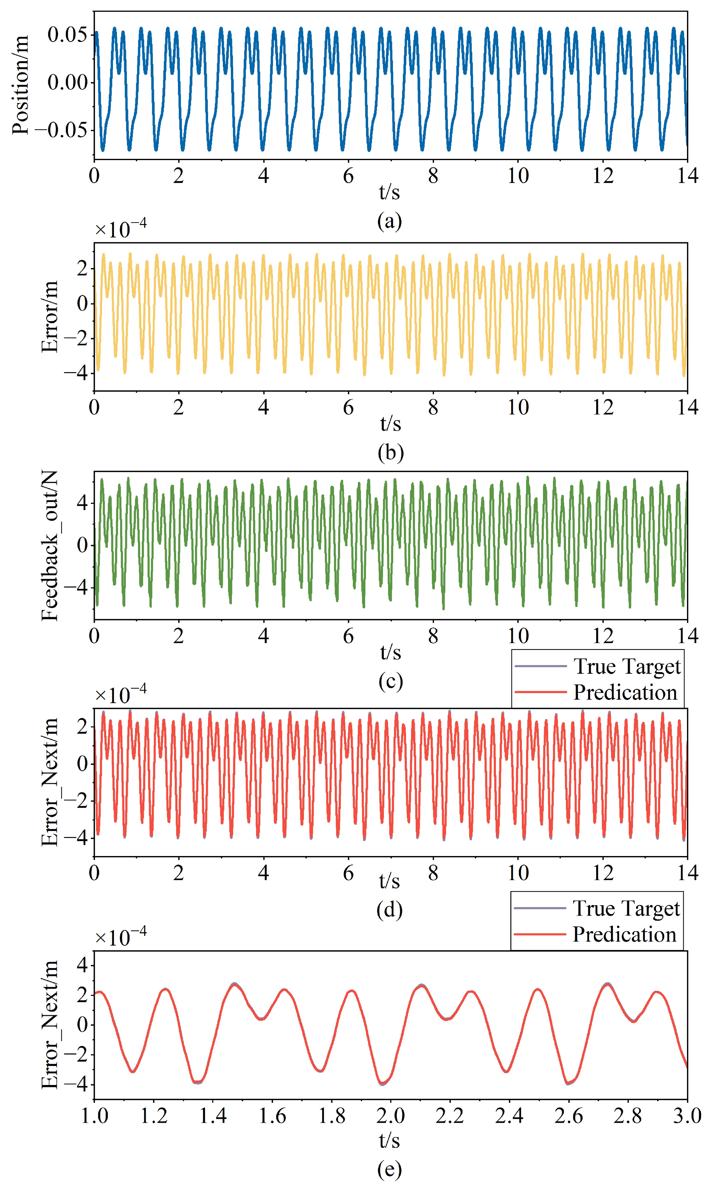Figure 6a,b, respectively, illustrate the displacement trajectory and the variation in tracking error during the motion process. During the segmented intervals of acceleration and deceleration, the system error exhibits fluctuations with appropriate amplitudes. As shown in Figure 6c, the feedback controller will dynamically modify in response to variations in inaccuracy to sustain high-precision positioning to the greatest extent practicable. Figure 6d juxtaposes the predicted values of the Parallel GRU–Transformer model with the actual tracking error, whereas Figure 6e elucidates the specifics of the localized region. The findings achieved are presented in

Table 2. R² and smape metrics for different models.

Neural Network Methods	R2	sMAPE
LSTM	0.9851	65.85%
GRU	0.9712	67.12%
Transformer	0.9985	12.23%
Parallel LSTM–Transformer	0.9973	14.05%
GRU–Transformer-A	0.9866	35.89%
GRU–Transformer-B	0.9574	47.31%
Parallel GRU–Transformer	0.9991	11.96%

Note: Bold indicates the best result.

in comparison to mainstream prediction models such as LSTM, GRU, Transformer, Parallel LSTM–Transformer, and GRU–Transformer architectures from Zheng et al. and Zhou et al., similar to our proposed structure [39,40].

Case 2—Random Multi-Sine Trajectory: To further examine the model’s adaptability in scenarios characterized by random and high-frequency disturbances, this study employs three sine functions with varying frequencies and phases to superimpose and create reference trajectories, thus constructing a complex input sequence with multi-scale fluctuations. The expression is displayed below (49). Subsequent experiments demonstrate that the Parallel GRU–Transformer continues to accurately forecast the error curve, exhibiting a strong correlation with the actual error, as illustrated in Figure 7, in comparison to the state-of-the-art prediction model, as illustrated in

Table 3. R² and smape metrics for different models.

Neural Network Methods	R2	sMAPE
LSTM	0.9894	23.85%
GRU	0.9813	29.12%
Transformer	0.9972	5.47%
Parallel LSTM–Transformer	0.9969	10.36%
GRU–Transformer-A	0.9981	12.68%
GRU–Transformer-B	0.9866	35.89%
Parallel GRU–Transformer	0.9985	4.85%

Note: Bold indicates the best result.

.

$$y\left(t\right)=0.02sin(30t-{\displaystyle \frac{\pi }{4}})+0.02sin(20t+{\displaystyle \frac{\pi }{2}})+0.05sin\left(10t\right)\left(m\right)$$

(49)

The experimental findings indicate that the Parallel GRU–Transformer network achieves high predictive accuracy across two distinct temporal modalities: a fourth-order polynomial trajectory and a random multi-sine trajectory. The trained network can generalize to different trajectory types and sustain stable error estimation under high-amplitude or high-frequency transitions, providing a promising basis for precise feedforward compensation and online dynamic correction. Furthermore, we conducted direct comparisons with the GRU–Transformer architectures proposed by Zheng et al. and Zhou et al., which adopt deeper encoder blocks and larger hidden dimensions, resulting in an inference latency of around $800\mathsf{\mu }\mathrm{s}$. While these models perform well in general scenarios, our approach achieves higher accuracy on the present dataset with a substantially lower inference latency of only $30\mathsf{\mu }\mathrm{s}$, making it more suitable for real-time embedded deployment in precision motion control.

3.3. Control Validation

The prior training results indicate that the developed neural network is capable of forecasting the subsequent error signal for the motion platform at a specified time. This research presents an extra feedforward compensation mechanism within the closed-loop control framework to attain dynamic compensation based on its predictive performance. The feedback loop employs a conventional PID controller to maintain high precision despite fluctuating operating conditions, owing to its strong regulatory capacity. The error information forecasted by the neural network for the subsequent moment is integrated into the nonlinear PD controller to deliver feedforward correction for the feedback output, thereby facilitating prompt compensation for potential deviations during the motion process.

The following common performance indices will be used to evaluate the quality of the control algorithms:

(1) The maximum value of the error and the absolute mean (AM), expressed as (50) and (51).

$$E_m=\underset{k\in [0,M-1]}{max}\left\{\left|e\right(k\left)\right|\right\}$$

(50)

$$E_{AM}={\displaystyle \frac{1}{M}}\sum _{k=0}^{M-1}\left|e\left(k\right)\right|$$

(51)

(2) The maximum value of the moving average (MA) and the absolute mean of the MA. MA is a dynamic metric employed to ascertain the average variance of data within a predetermined window, emphasizing the overarching trend, expressed as (52) and (53).

$$M{A}_m=\underset{i\in [0,M-1]}{max}\left({\displaystyle \frac{1}{N}}\sum _{k=i-N+1}^i\left|e\left(k\right)\right|\right)$$

(52)

$$M{A}_{AM}={\displaystyle \frac{1}{M}}\sum _{i=0}^{M-1}\left({\displaystyle \frac{1}{N}}\sum _{k=i-N+1}^i\left|e\left(k\right)\right|\right)$$

(53)

(3) The maximum value of moving standard deviation (MSD) and the absolute mean of MSD. The MSD represents the standard deviation of data inside a sliding window, reflecting the extent of data variability. A greater standard deviation indicates more significant oscillations in the data, expressed as (54) and (55).

$$MS{D}_m=\underset{i\in [0,M-1]}{max}\left(\sqrt{{\displaystyle \frac{1}{N}}\sum _{k=i-N+1}^i{\left|e\left(k\right)-M{A}_i\right|}^2}\right)$$

(54)

$$MS{D}_{AM}={\displaystyle \frac{1}{M}}\sum _{i=0}^{M-1}\left(\sqrt{{\displaystyle \frac{1}{N}}\sum _{k=i-N+1}^i{\left|e\left(k\right)-M{A}_i\right|}^2}\right)$$

(55)

where T represents the total running time of the relevant experimental section, $\mathsf{\Delta }t$ represents the sampling time, $M=T/t$, M is the number of sampling points, N is the size of the sliding window, $e\left(k\right)$ is the kth error value in the time series, i is the discrete sampling point index, and $M{A}_i$ represents the $MA$ at the ith sampling point.

Based on the actual needs of the laboratory, this study set the window size to $N=100$ and selected PID feedback control and a combination of model-based feedforward compensation and PID feedback control strategies as control benchmarks to compare and evaluate the performance of the proposed Parallel GRU–Transformer-based feedforward compensation method. This research also illustrated the effect of Parallel GRU–Transformer-based feedforward compensation on the main controller’s output.

S1: PID Feedback. This method employs a typical parallel PID controller, represented by its transfer function as (56).

$$C\left(s\right)=K_p+{\displaystyle \frac{K_i}{s}}+K_{d}s$$

(56)

The PID parameters are configured as $K_p=850$, $K_i=250$, and $K_d=50$, which were determined through extensive experimental tuning to achieve an optimal balance between tracking accuracy, stability, and robustness under various operating conditions.

S2: Model-based feedforward compensation utilizing PID feedback. The feedforward structure employs velocity and acceleration feedforward compensation derived from the system’s inverse model, optimizing dynamic performance by suitably adjusting the compensation coefficient, thereby enhancing trajectory tracking of the controlled object.

S3: Parallel GRU–Transformer-based feedforward compensation with PID feedback. The feedforward compensation control algorithm provided in this paper is used, and the speed and acceleration feedforward compensation are the same as in S2. To achieve a balance between high sensitivity and rapid convergence in both small- and large-error domains, the parameter ranges were determined based on the prior literature and preliminary simulations, followed by a grid search with performance evaluations on multiple reference trajectories to ensure stability, accuracy, and actuator smoothness. Extensive experimentation led to the final determination of the nonlinear PD controller parameters: the proportional gain coefficient ${\beta }_1$ is 10,000, the differential gain coefficient ${\beta }_2$ is 200, and the nonlinear amplitude adjustment parameters are ${\alpha }_1=0.5$ and ${\alpha }_2=1.5$, with a segmentation threshold $\delta$ of $0.00005$.

This presents the control effects of the identical fourth-order polynomial trajectory and random multiple-sine trajectory as utilized in the prediction validation.

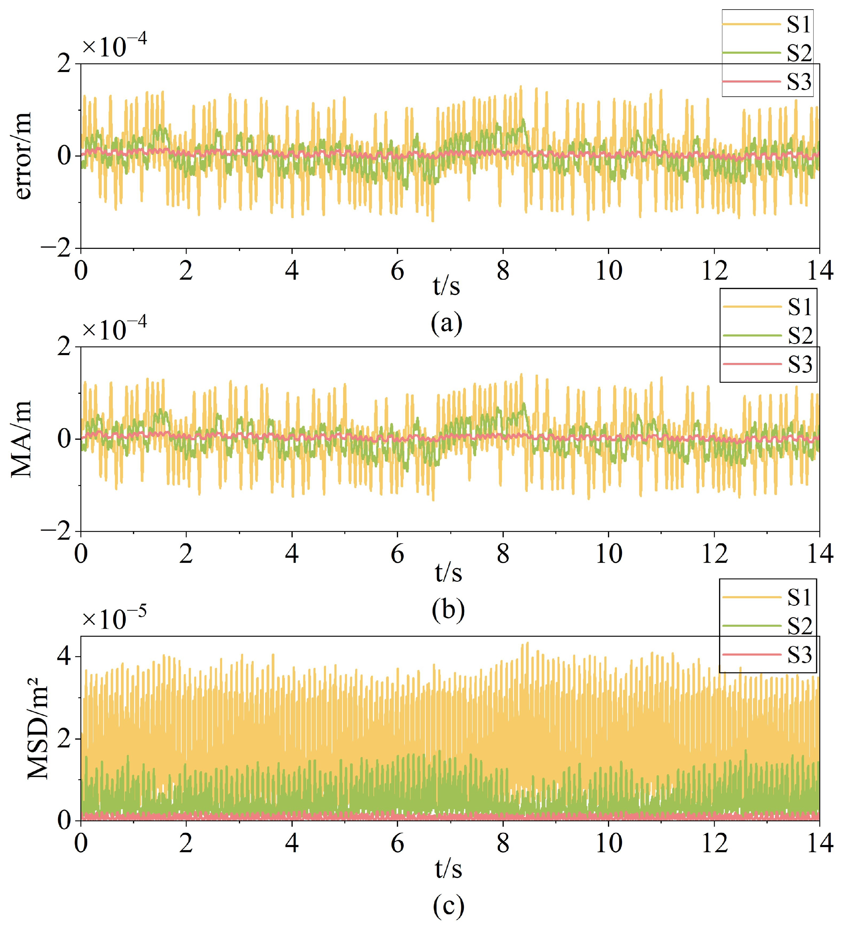
Case 1—Fourth-order polynomial trajectory: Figure 8 illustrates the tracking error along with its respective moving averages (MAs) and mean square deviations (MSDs) across various control methods, while

Table 4. Tracking performance indexes.

CaseI	S1	S2	S3
$E_m({10}^{-4}$m)	1.52	0.79	0.18
$E_{MAE}({10}^{-5}$m)	4.67	2.37	0.56
$M{A}_m({10}^{-4}$m)	1.41	0.78	0.17
$M{A}_{MAE}({10}^{-5}$m)	4.45	2.3	0.55
$MS{D}_m({10}^{-5}$m2	4.35	1.72	0.25
$MS{D}_{MAE}({10}^{-5}$m2	1.79	0.53	0.09

Note: Bold indicates the best result.

enumerates the different indicators. The results showed that S3 was superior to S2 and S1 in all indications, with an $MS{D}_m$ of $2.5\times {10}^{-6}$ m² for S3, which was nearly 1/7 lower than S2’s $1.72\times {10}^{-5}$ m². Figure 9a illustrates that the feedforward compensation output derived from Parallel GRU–Transformer predictions supplants the primary control responsibilities of the PID controller during most intervals, thereby markedly diminishing the workload and error magnitude of the main controller. M1 represents feedforward compensation output based on the Parallel GRU–Transformer, and M2 represents the PID controller output.

Case 2—Random Multiple-Sine Trajectory: This case involves conducting comparative experiments to evaluate the performance of tracking random multiple-sine curves. Similarly, Figure 10 displays the error curves, MA, and MSD under different techniques;

Table 5. Tracking performance indexes.

CaseII	S1	S2	S3
$E_m({10}^{-4}$m)	4.13	1.75	0.66
$E_{MAE}({10}^{-4}$m)	1.78	0.66	0.29
$M{A}_m({10}^{-4}$m)	4.09	1.71	6.43
$M{A}_{MAE}({10}^{-5}$m)	1.77	0.65	0.29
$MS{D}_m({10}^{-5}$m2	9.71	3.77	1.83
$MS{D}_{MAE}({10}^{-5}$m2)	2.66	1.08	0.47

Note: Bold indicates the best result.

summarizes the important performance measures. From the data, it can be seen that S3 still has significant advantages, with an $MS{D}_{AM}$ value of only $4.7\times {10}^{-6}{\mathrm{m}}^2$, which is less than half of S2’s $1.08\times {10}^{-5}{\mathrm{m}}^2$. As shown in Figure 9b, the Parallel GRU–Transformer-based feedforward output still bears most of the control energy in this environment, effectively reducing the output pressure of the PID.

4. Conclusions

In conclusion, the nonlinear PD feedforward compensation strategy based on Parallel GRU–Transformer prediction can significantly reduce the tracking error as well as the moving average (MA) and moving standard deviation (MSD) of motion errors under two completely different trajectory conditions, without requiring an accurate model of the controlled system. Additionally, the strategy effectively reduces the workload of the main controller. Due to the low dimensionality of network input features, the training process is straightforward and efficient. On our experimental device, the trained model has a small computational footprint, and inference completes within $30\mathsf{\mu }\mathrm{s}$, fully within the control-cycle budget, indicating that the method can be deployed without significant additional resources while meeting real-time requirements. These advantages suggest that the method has a certain level of robustness and good generalization capability, making it suitable for high-precision motion control tasks in fields such as semiconductor equipment and precision robotics, with broad prospects for practical engineering use and potential for extension to other industrial applications.