Nonparametric Transformation Models for Double-Censored Data with Crossed Survival Curves: A Bayesian Approach

Abstract

Double-censored data are frequently encountered in pharmacological and epidemiological studies, where the failure time can only be observed within a certain range and is otherwise either left- or right-censored. In this paper, we present a Bayesian approach for analyzing double-censored survival data with crossed survival curves. We introduce a novel pseudo-quantile I-splines prior to model monotone transformations under both random and fixed censoring schemes. Additionally, we incorporate categorical heteroscedasticity using the dependent Dirichlet process (DDP), enabling the estimation of crossed survival curves. Comprehensive simulations further validate the robustness and accuracy of the method, particularly under the fixed censoring scheme, where traditional approaches may NOT be applicable. In the randomized AIDS clinical trial, by incorporating the categorical heteroscedasticity, we obtain a new finding that the effect of baseline log RNA levels is significant. The proposed framework provides a flexible and reliable tool for survival analysis, offering an alternative to parametric and semiparametric models.

1. Introduction

A large body of statistical research in biomedicine has focused on right-censored data due to its prevalence, while less emphasis has been placed on other less common types of censored data, such as left- or interval-censored data. Left censoring occurs when the event time precedes the recruitment time, whereas (Case 2) interval censoring occurs when the event time of interest is only known to fall within a certain interval. Left and right censoring can be viewed as special cases of interval censoring. A more complicated censoring mechanism may involve more than one type of censoring in the sample or a mixture of uncensored and censored subjects. For instance, “partly interval-censored data” [1,2] arise when some failure times are interval-censored while others are uncensored. This paper studies another special type of survival data called “double-censored data” [3], in which the subjects are uncensored within a specific time interval and the subjects are either left- or right-censored when their actual event times fall outside the time interval. Due to the complex data structure and limited information, contemporary statistical methods for double-censored data are still underdeveloped and often inefficient, posing significant challenges to statistical inference, including accurate estimation and prediction. Double-censored data commonly arise in biomedical, pharmacological, and epidemiological studies [4,5]. A specific example is the randomized AIDS clinical trial [6] which aimed to compare the responses of HIV-infected children to three different treatments. The outcome variable of interest is the plasma HIV-1 RNA level (instead of a conventional “time” variable) as a measure of the viral load. The plasma HIV-1 RNA level, given by the NucliSens assay, is considered double-censored because its measurement can be highly unreliable below 400/mL or above 75,000/mL of plasma. In other words, this variable is observable only within the range of 400/mL to 75,000/mL and is left- or right-censored otherwise. To avoid ambiguity, it is remarked that “double censoring” has also been used in literature to describe another type of censoring mechanism in survival analysis, where both the time origin and event time are potentially interval-censored [7]. We adopt the first definition of “double censoring” above.

The term “double censoring” was first pinpointed by [3]. Following his research work  [8] proposed a self-consistent nonparametric maximum likelihood estimator (NPMLE) of the survival function based on double-censored data. Refs.  [9,10] later studied the weak convergence and asymptotic properties of the NPMLE, respectively. Refs. [11,12] developed algorithms tailored to the computation of the NPMLE. In the presence of covariates, a natural way to incorporate them into the analysis is to assume the Cox proportional hazards (PH) model [13]. For instance, Ref. [14] studied the nonparametric maximum likelihood estimation for the Cox PH model and the asymptotic properties of the estimator based on double-censored data. Ref. [15] later proposed to obtain the MLE based on the EM algorithm and approximated likelihood, which was shown to be more numerically stable and computationally efficient.

However, the proportional hazards model may be restrictive in practical applications. Therefore, it is worth considering the semiparametric transformation model [16,17,18,19] as an alternative because of its higher flexibility to cover Cox’s PH and PO models. With double-censored data, Ref. [20] (further in text Li2018) studied the nonparametric maximum likelihood estimation (NPMLE) of the semiparametric transformation model that allowed for possibly time-dependent covariates, and they proposed to use an EM algorithm to obtain the NPMLE. This route of semiparametric transformation models requires full model identifiability by assuming the model error distribution to be known or parametric, similar to the main stream of transformation model literature [19,21,22,23,24]. Despite its convenience, this strategy may encounter model misspecification (refer to the numerical studies in [25] for examples).

Compared with semiparametric transformation models, the nonparametric transformation models [26,27,28,29,30] are robust since they allow both the transformation and model error distribution to be unspecified and nonparametric. Nonetheless, to address the identifiability issue, most of the existing literature imposed complicated identification constraints on the two nonparametric components, leading to infeasible computation. To balance the model robustness and computational feasibility, ref. [25] studied the reliable Bayesian predictive inference under nonparametric transformation models with both transformation and model error unidentified. Nonetheless, they only focus on right-censored data. To the best of our knowledge, there have not yet been studies on nonparametric transformation models with double-censored data.

Furthermore, most of the existing literature studied the random censoring scheme only, and excluded the fixed censoring scheme. The fixed censoring scheme, where the observations are censored with two fixed points, usually does not provide much useful information because the dataset can have many duplicate values. This scheme is a common practice in clinical trials, for example, the randomized AIDS clinical trial studied in this paper.

Besides the lack of research on the fixed censoring scheme, most of the existing literature on transformation models [20,25,26,28,31,32] assumes that the model error is independent of covariates, indicating that they can NOT model crossed survival curves. Ref. [33] introduces a semiparametric random-effects linear transformation model to estimate the crossed survival curves, while they still need to assume the density of model error to be known.

Based on the above literature review, we are driven to extend the Bayesian method by [25] to the double censoring scheme, especially the fixed censoring scheme, and introduce a special model for categorical heteroscedasticity in the sense that the model error distributions depend on the categorical covariates. Our method addresses two key challenges: (i) modeling the monotone transformation under the double censoring scheme, especially with fixed censored data; (ii) incorporating the categorical heteroscedasticity nonparametrically so as to estimate crossed survival curves.

To address the first challenge, we inherit and modify the quantile-knot I-splines [25,34] prior. For the random censoring scheme, we straightforwardly interpolate the interior knots of I-splines from the quantiles of left- and right-censoring endpoints. However, this interpolation strategy is not applicable to the fixed censoring scheme since the quantiles of censored endpoints do NOT exist anymore. We propose a novel pseudo-quantile I-splines prior for the transformation under fixed censoring by synthesizing the exact survival times and interpolating the knots of I-splines at the average of the pseudo quantiles of the synthesized data. Numerical studies demonstrate that the proposed pseudo-quantile modeling effectively captures the true distribution of the variable of interest and extracts potentially hidden information that is lost due to fixed censoring. To address the second challenge, we borrow the strength from the Dependent Dirichlet process (DDP) proposed by [35]. Specifically, we employ the ANOVA DPP [36] to model the dependency of the model error and the categorical covariates. Introducing the categorical heteroscedasticity through DDP does not change the quantile-knot i-spline modeling, making the computation by Markov Chain Monte Carlo (MCMC) still feasible and reliable. We have summarized all the symbols used in this paper in Table 1.

Table 1. List of symbols.

Notation	Definition
$T_i$	True time-to-event data
$Z_i$	p-dimensional covariate vector
$X_i$	q-dimensional Categorical covariate vector
$L_i,R_i$	Left/right censoring data
$\widetilde{T_i}$	Observed time-to-event data
${\delta }_{i1},{\delta }_{i2},{\delta }_{i3}$	Indicators for left-censored/uncensored/right-censored
$H(·)$	The nonnegative monotone transformation
$\beta$	The vector of regression coefficients
$\xi$	The multiplicative model error in transformation model
$B_j\left(t\right)$	I-spline basis
N	The number of knots in I-splines functions
$\tau$	Maximum observed time
${\widehat{Q}}_X\left(p\right)$	Empirical quantile function for variable X

The major contributions of this paper are summarized as follows.

• Contribute a novel method for survival prediction under nonparametric transformation models with double-censored data, especially for the fixed censoring scheme.
• Incorporate categorical heteroscedasticity in nonparametric transformation models so as to model crossed survival curves.
• With categorical heteroscedasticity, evidence the significance of the effect of baseline log (RNA) levels in the randomized AIDs clinical trial.

The remainder of this paper is organized as follows. We introduce our data structure and model in Section 2. Our proposed innovative priors will be explained in detail in Section 3. A special case where the model error distributions depend on the categorical covariates is discussed in Section 4. Posterior inference and estimation will be explored in Section 5. Simulation results will be presented in Section 6. We also apply our method to real data in Section 7. A discussion will be given in Section 8.

2. Data, Model, and Assumptions

2.1. Data Structure

Here, we describe the typical data structure of doubly censored data in survival analysis. Consider a study that involves n independent subjects. For subject i, let $T_i$ denote the time-to-event and $Z_i$ be the p-dimensional vector of time-invariant covariates. The time-to-event $T_i$ can only be observed between $L_i$ and $R_i$, and if not observed, it is either left-censored at $L_i$ or right-censored at $R_i$. Define ${\delta }_{i1}=I(T_i\le L_i)$, ${\delta }_{i2}=I(L_i<T_i\le R_i)$, ${\delta }_{i3}=I(R_i<T_i)$, where $I(·)$ is the indicator function. Then, it follows ${\delta }_{i1}+{\delta }_{i2}+{\delta }_{i3}=1$. The observed data are of the form $\{({\tilde{T}}_i,L_i,R_i,Z_i,{\delta }_{i1},{\delta }_{i2},{\delta }_{i3});i=1,\dots ,n\}$, where ${\tilde{T}}_i=\max \{L_i,\min (R_i,T_i)\}$ is the observed time-to-event for subject i. Here, we assume that $L_i=0$ if ${\delta }_{i3}=1$ and $R_i=\infty$ if ${\delta }_{i1}=1$, since such information is generally not available, for better data organization. Furthermore, $T_i$ and $(L_i,R_i)$ are assumed to be conditionally independent given $Z_i$ (noninformative censoring) as common practice.

2.2. Nonparametric Transformation Models

We consider a class of linear transformation models, which relate the time-to-event to the relative risk in a multiplicative way as follows:

$$H\left(T\right)=\xi exp\left({\beta }^{\mathrm{T}}Z\right),$$

(1)

where $H(·)$ is a strictly increasing transformation function that is positive on ${\mathbb{R}}^{+}$, $\beta$ is the p-dimensional vector of regression coefficients coupling Z, and $\xi$ is the model error with distribution function $F_{\xi }$. The above transformation model is considered a nonparametric transformation model when the functional forms of both $H(·)$ and $F_{\xi }$ are unknown. As mentioned earlier, model nonidentifiability would mean that different sets of ($H,F_{\xi },\beta$) can generate an identical likelihood function. For the rest of this paper, Model (1) will be treated as a nonparametric transformation model, henceforth NTM.

The NTM is obtained by applying an exponential transformation to a class of linear transformation models with additive relative risk.

$$h\left(T\right)={\beta }^{\mathrm{T}}Z+ϵ,$$

(2)

where $h(·)=log\left(H\right(·\left)\right)$ and $ϵ=log\left(\xi \right)$. This transformation is necessary since the transformation function $h(·)$ in Model (2) is sign-varying on ${\mathbb{R}}^{+}$, which leads to insoluble problems regarding prior elicitation and posterior sampling. After the transformation, $H(·)$ is strictly positive on ${\mathbb{R}}^{+}$, thus allowing the NTM to avoid the above problems.

3. Likelihood and Priors

3.1. Likelihood Function

Given observed data $\{({\tilde{T}}_i,L_i,R_i,Z_i,{\delta }_{i1},{\delta }_{i2},{\delta }_{i3});i=1,\dots ,n\}$, we can construct the likelihood function as

$$\begin{array}{ccc}\hfill \mathcal{L}\left(H,F_{\xi },\beta \mid \tilde{T},Z,{\delta }_1,{\delta }_2,{\delta }_3\right)& =& \prod _{i=1}^n{\left[F_{\xi }\left\{H\left({\tilde{T}}_i\right)e^{-{\beta }^{\mathrm{T}}{Z}_i}\right\}\right]}^{{\delta }_{i1}}\hfill \\ & & \times {\left[f_{\xi }\left\{H\left({\tilde{T}}_i\right)e^{-{\beta }^{\mathrm{T}}{Z}_i}\right\}{H}^{\prime }\left({\tilde{T}}_i\right)e^{-{\beta }^{\mathrm{T}}{Z}_i}\right]}^{{\delta }_{i2}}\hfill \\ & & \times {\left[S_{\xi }\left\{H\left({\tilde{T}}_i\right)e^{-{\beta }^{\mathrm{T}}{Z}_i}\right\}\right]}^{{\delta }_{i3}},\hfill \end{array}$$

(3)

where $f_{\xi }(·)=F_{\xi }^{\prime }(·)$ is the density function of $\xi$ and $S_{\xi }(·)=1-F_{\xi }(·)$ is the survival function of $\xi$.

3.2. Dirichlet Process Mixture Model

To characterize model error in the NTM, we choose the common Dirichlet process mixture (DPM) models [37] as the priors for $f_{\xi }$ and $S_{\xi }$. In this paper, we adopt the truncated stick-breaking construction [38] of the DPM.

$$f_{\xi }(·)=\sum _{l=1}^L{p}_l{f}_w({\psi }_l,{\nu }_l),S_{\xi }(·)=1-\sum _{l=1}^L{p}_l{F}_w({\psi }_l,{\nu }_l),$$

(4)

where $f_w(\psi ,\nu )$ and $F_w(\psi ,\nu )$ are the density and distribution functions of a Weibull distribution, respectively. The Weibull distribution is selected as the DPM kernel for two reasons: (i) it is flexible to various hazard shapes [39]; (ii) the Weibull kernel guarantees the properness of the posterior under the unidentified transformation models (refer to [25] for details).

In explicit form, the stick-breaking weights $p_l$ and the parameters $({\psi }_l,{\nu }_l)$ are generated as follows

$$p_l=q_k\prod _{k=1}^{L-1}(1-q_k),q_k\sim \mathrm{Beta}(1,c),{\psi }_l\sim \mathrm{Gamma}(1,1),{\nu }_l\sim \mathrm{Gamma}(1,1).$$

(5)

Throughout this paper, we specify $c=1$ in the DPM prior, which is a commonly used default choice [40]. The choice of L is relatively flexible. Since the theoretical total-variation error between the truncated DP and the true DP is bounded by $4nexp\{-(L-1)/c\}$ [41], we suggest the readers adopt a suitable truncation level based on the data size.

3.3. Pseudo-Quantile I-Splines Prior

Regarding the transformation function of the NTM and its derivative, we rely on a type of I-spline priors to capture the relevant information. To construct such priors, we first take $\tau ={\max }_i\left({\tilde{T}}_i\right)$ to be the largest observed time-to-event in the sample, then $D=(0,\tau ]$ is the interval that contains all observed time-to-events. Note that $H(·)$ is differentiable on D, thus we can model $H(·)$ and $H^{\prime }(·)$ by

$$H\left(t\right)=\sum _{j=1}^K{\alpha }_j{B}_j\left(t\right),H^{\prime }\left(t\right)=\sum _{j=1}^K{\alpha }_j{B}_j^{\prime }\left(t\right),$$

(6)

where ${\left\{{\alpha }_j\right\}}_{j=1}^K$ are positive coefficients, ${\left\{B_j\right\}}_{j=1}^K$ are I-spline basis functions [34] on D, and ${\left\{B_j^{\prime }\right\}}_{j=1}^K$ are the corresponding derivatives.

The number of I-spline basis functions $K=N+r$, where N is the total number of interior knots and r is the order of smoothness, with $(r-1)$th order derivative existing. We adopt the default value of $r=4$ in R package splines2.

Then, it becomes our primary task to specify the exact number of interior knots and pinpoint their locations. One logical way to approach this task is to base the selection of interior knots on empirical quantiles of the collected data. In doing so, we can effectively utilize useful knowledge inherent to the distribution of the observed time-to-events.

Let ${\widehat{F}}_X\left(t\right)=n^{-1}{\sum }_{i=1}^{n}I(X_i\le t)$ be the empirical distribution function of some variable X and ${\widehat{Q}}_X\left(p\right)=inf\{t:p\le {\widehat{F}}_X\left(t\right)\}$ be the corresponding empirical quantile function, where X can be equivalently replaced by T, $\tilde{T}$, or other random variables. Note that since the exact (actual) time-to-events T cannot always be observed, ${\widehat{F}}_T(·)$ and ${\widehat{Q}}_T(·)$ can only be constructed based on the subset of the observed data with ${\delta }_{i2}=1$ (i.e., where the exact time-to-events are observed). We first consider knot selection via empirical functions under the random censoring setting, which is very often the assumed setting in related literature.

3.3.1. Random Censoring Knot Selection

Define ${\tilde{T}}_L=\{{\tilde{T}}_i\in \tilde{T}:{\delta }_{i3}=0\}$ and ${\tilde{T}}_R=\{{\tilde{T}}_i\in \tilde{T}:{\delta }_{i1}=0\}$. Let $N_I$ be the initial number of knots. The interior knot selection procedure can be described as follows.

• Step 1: Choose $N_I$ empirical quantiles of exact time-to-events as interior knots, where each knot $t_j={\widehat{Q}}_T\{j/(N_I-1)\}$ and $j=0,\dots ,N_I-1$, such that $0<t_0<\dots <t_{N_I-1}\le \tau$.
• Step 2: For $j=0,\dots ,N_I-1$, if $\mid {\widehat{F}}_T\left(t_j\right)-{\widehat{F}}_{{\tilde{T}}_L}\left(t_j\right)\mid \ge 0.05$, interpolate a new knot $t_j^{*}={\widehat{Q}}_{{\tilde{T}}_L}\{j/(N_I-1)\}$.
• Step 3: For $j=0,\dots ,N_I-1$, if $\mid {\widehat{F}}_T\left(t_j\right)-{\widehat{F}}_{{\tilde{T}}_R}\left(t_j\right)\mid \ge 0.05$, then interpolate another new knot $t_j^{**}={\widehat{Q}}_{{\tilde{T}}_R}\{j/(N_I-1)\}$.
• Step 4: Sort all the chosen and interpolated knots $\{t_0,\dots ,t_j,t_j^{*},t_j^{**},\dots ,t_{N_I-1}\}$ in ascending order resulting in the final selected interior knots.

It is worth noting that only exact time-to-events can provide information about $H^{\prime }$, therefore the initial interval knots are chosen by equally spaced empirical quantiles of T, i.e.,${\tilde{T}}_i$ for ${\delta }_{i2}=1$. To mitigate the lack of information when the percentage of left or right-censored observations is high, extra interior knots are generated as needed.

The problem of interior knot selection becomes much more complex and difficult under fixed censoring. In such circumstances, the empirical distributions of observed time-to-events would heavily gravitate toward the fixed censoring points, making interpolation of additional interior knots infeasible. Therefore, in cases of high censoring, attempts have to be made to extract some information from the unobserved time-to-events. Thus, we propose a novel method for effective interior knot selection that synthesizes pseudo data to mimic the distribution of unobserved time-to-events. This innovative method then leads to a new type of prior for the transformation function, which we name the “pseudo-quantile I-splines prior” (PQI prior).

3.3.2. Fixed Censoring Knot Selection

Fixed censoring occurs when $L_{i_1}=L$ for $i_1=1,\dots ,n_1$ and $R_{i_2}=R$ for $i_2=1,\dots ,n_2$, where $n_1$ and $n_2$ are the numbers of left-censored and right-censored observations, respectively, and L and R are some finite constants. Define $n_3=n-n_1-n_2$. The specification procedure can be described as follows.

For $k=1,\dots ,K$ (Steps 1–3),

• Step 1 (pseudo-left-censored data generation):
  Generate pseudo observations $({\mathcal{T}}_{L_{k1}},\dots ,{\mathcal{T}}_{L_{k{i}_1}},\dots ,{\mathcal{T}}_{L_{k{n}_1}})$ from some distribution (e.g., Weibull, gamma) such that all ${\mathcal{T}}_{L_{k{i}_1}}<L$.
• Step 2 (pseudo-right-censored data generation):
  Generate pseudo observations $({\mathcal{T}}_{R_{k1}},\dots ,{\mathcal{T}}_{R_{k{i}_2}},\dots ,{\mathcal{T}}_{R_{k{n}_2}})$ from the same distribution such that all ${\mathcal{T}}_{R_{k{i}_2}}>R$.
• Step 3 (pseudo-quantile computation):
  Let ${\mathcal{T}}_k=({\mathcal{T}}_{L_{k1}},\dots ,{\mathcal{T}}_{L_{k{n}_1}})\cup (T_1,\dots ,T_{n_3})\cup ({\mathcal{T}}_{R_{k1}},\dots ,{\mathcal{T}}_{R_{k{n}_2}})$. Compute ${\widehat{F}}_{{\mathcal{T}}_k}\left(t\right)=n^{-1}$${\sum }_{i=1}^{n}I({\mathcal{T}}_{ki}\le t)$ and ${\widehat{Q}}_{{\mathcal{T}}_k}\left(p\right)=inf\{t:p\le {\widehat{F}}_{{\mathcal{T}}_k}\left(t\right)\}$.
• Step 4 (quantile averaging):
  Compute ${\widehat{Q}}_{\mathcal{T}}\left(p\right)=K^{-1}{\sum }_{k=1}^K{\widehat{Q}}_{{\mathcal{T}}_k}$. Choose N averaged empirical quantiles of the combined time-to-events as interior knots, where each knot $t_j={\widehat{Q}}_{\mathcal{T}}\{j/(N-1)\}$ and $j=0,\dots ,N-1$. Output this series $\{t_0,\dots ,t_j,\dots ,t_{N-1}\}$ as the finally selected interior knots.

In Step 4, one can show that with sufficiently large N, the inserted pseudo quantiles become stable, and thus, the induced I-spline basis is also stable. These pseudo-quantile knots are also combined with the exact time-to-events that are observed for completeness. The averaged empirical quantiles should closely imitate the true quantiles of the exact time-to-events (observed and unobserved), and thus, the selected interior knots should provide reliable and sufficient information. Any pre-existing knowledge about the potential distribution of the exact time-to-events could help facilitate the selection process and refine the results.

4. Transformation Models with Crossed Survival Curves

In this section, we extend the model (1) to a special case where the model error distributions depend on the categorical covariates. Assume one or q-dimensional categorical covariates X with a total of G categories. For example, if there is only one covariate, K equals the number of categories of that covariate; if there are multiple variables, one-hot encoding can be used, and G equals the product of the categories of each covariate. The model error distributions depend on the categorical covariates, indicating that the survival curves of different categories will be crossed. And we introduce the following models

$$H\left(T\right|x=g)={\xi }_{g}exp\left({\beta }^{\mathrm{T}}Z\right),g=1,...,G,$$

(7)

where ${\xi }_g$ is the model error under group k with distribution function $F_{{\xi }_g}$. That is, we assume that within different categories, the distribution of the model error exhibits heterogeneity. Similarly, we denote that $h(·)=log\left(H\right(·\left)\right)$ and ${ϵ}_k=log\left({\xi }_g\right)$. And (7) can be written as $h\left(T\right|x=g)={\beta }^{\mathrm{T}}Z+{ϵ}_g,g=1,...,G$. Given observed data $\{({\tilde{T}}_i,L_i,R_i,Z_i,X_i,{\delta }_{i1},{\delta }_{i2},{\delta }_{i3});$ $i=1,\dots ,n\}$, we can construct the likelihood function as

$$\begin{array}{ccc}\hfill \mathcal{L}\left(H,F_{{\xi }_g},\beta \mid \tilde{T},Z,X,{\delta }_1,{\delta }_2,{\delta }_3\right)& =& \prod _{g=1}^G\prod _{i=1}^n{\left[F_{{\xi }_g}\left\{H\left({\tilde{T}}_i\right)e^{-{\beta }^{\mathrm{T}}{Z}_i}\right\}\right]}^{{\delta }_{i1}}\hfill \\ & & \times {\left[f_{{\xi }_g}\left\{H\left({\tilde{T}}_i\right)e^{-{\beta }^{\mathrm{T}}{Z}_i}\right\}{H}^{\prime }\left({\tilde{T}}_i\right)e^{-{\beta }^{\mathrm{T}}{Z}_i}\right]}^{{\delta }_{i2}}\hfill \\ & & \times {\left[S_{{\xi }_g}\left\{H\left({\tilde{T}}_i\right)e^{-{\beta }^{\mathrm{T}}{Z}_i}\right\}\right]}^{{\delta }_{i3}},\hfill \end{array}$$

(8)

where $f_{{\xi }_g}(·),F_{{\xi }_g}(·),S_{{\xi }_g}(·)$ are the density function, the cumulative distribution function, and the survival function of ${\xi }_g$, respectively. Compared with the likelihood function (3), (8) includes the product of the likelihood functions for each category.

ANOVA Dependent Dirichlet Process Prior

The DPM prior will no longer be applicable where the model error distributions depend on the categorical covariates. Ref. [35] defined the dependent Dirichlet process (DDP) to allow a regression on a covariate X. Since the K categories, We here specify appropriate nonparametric ANOVA DDP priors [36] for $f_{{\xi }_g}(·),F_{{\xi }_g}(·)$, and $S_{{\xi }_g}(·)$. Since they can be easily derived from one to the other, we here only introduce the priors for $F_{{\xi }_g}(·).$ Following [42], we write the stick-breaking form of $F_{{\xi }_g}={\sum }_{h=1}^{\infty }{w}_h\delta \left({\theta }_{gh}\right)$ for $gk=1,..,G$. And We impose additional structure on the locations ${\theta }_{gh}$ :

$${\theta }_{gh}=m_h+A_{gh},$$

where $m_h$ denotes the ANOVA effect shared by all the observations, and the terms of $A_{gh}$ are the ANOVA effects of different categories. For example, the locations are ${\theta }_{1h}=m_h+A_{1h},$ ${\theta }_{2h}=m_h+A_{2h}$ if $G=2$. For each category, they have a similar term $m_h$ shared by all the observations, and different $A_{1g}$ and $A_{2g}$ depict the heterogeneity under different categories.

5. Posterior Inference

5.1. Posterior Prediction and Nonparametric Estimation

Given the prior settings, the nonparametric parts of (1), specifically, the functionals H and $S_{\xi }$ can be represented by elements in $(\alpha ,p,\psi ,\nu )$, where $\alpha ={\left\{{\alpha }_j\right\}}_{j=1}^K$, $p={\left\{p_l\right\}}_{l=1}^L$, $\psi ={\left\{{\psi }_l\right\}}_{l=1}^L$, and $\nu ={\left\{{\nu }_l\right\}}_{l=1}^L$. Let $\Theta =(\beta ,\alpha ,p,\psi ,\nu )$ be the collection of all unknown parameters. The estimators of $(H,\beta ,S_{\xi })$ can then be obtained through the posterior distribution of $\Theta$.

First, we set the priors for parameters in $\Theta$ as (recall (5))

$$\begin{array}{cc}\hfill & {\alpha }_j\sim exp\left(\eta \right),\pi \left(\beta \right)\propto 1,\hfill \\ \hfill & p_l=q_k\prod _{k=1}^{L-1}(1-q_k),q_k\sim \mathrm{Beta}(1,c),l=1,\dots ,L-1;p_L=1-\sum _{l=1}^{L-1}{p}_l,\hfill \\ \hfill & G_0({\psi }_l,{\nu }_l)=\mathrm{Gamma}(1,1)\times \mathrm{Gamma}(1,1),\hfill \end{array}$$

(9)

where $\pi (·)$ is a prior density and $G_0$ is the base measure for the DPM prior. The posterior density of $\Theta$ can then be represented as

$$\pi (\Theta \mid \tilde{T},Z,{\delta }_1,{\delta }_2,{\delta }_3)\propto \mathcal{L}(\Theta \mid \tilde{T},Z,{\delta }_1,{\delta }_2,{\delta }_3)\pi \left(\beta \right)\pi \left(\alpha \right)\pi \left(p\right)\prod _{l=1}^L{G}_0({\psi }_l,{\nu }_l).$$

(10)

In the above prior setting, the hyperparameter $\eta$ can be dependent on other hyperparameters or fixed to some constant based on existing knowledge. It is, however, recommended that the mass parameter of the Beta distribution be fixed as $c=1$ and the base measure $G_0$ also be fixed as above.

It should be noted that the prior choice for $\beta$ is the improper uniform prior. Such a choice simplifies the posterior form and accelerates MCMC sampling. Under mild conditions, the posterior in (10) is still guaranteed to be proper. The NUTS (No-U-Turn Sampler) from Stan [43] is implemented to achieve posterior sampling. After sufficient sampling procedures, the posterior predictive survival probability of any future time-to-event $T_0$ can be obtained given some vector of covariates $Z_0$.

For such a prediction of a future time-to-event, denote the corresponding conditional posterior predictive survival probability as $S_{T_0\mid Z_0}\left(t\right)$. Mathematically, $S_{T_0\mid Z_0}\left(t\right)$ can be calculated through

$$\begin{array}{cc}\hfill S_{T_0\mid Z_0}\left(t\right)& =\int S_{T_0\mid Z_0}(t\mid \Theta )\pi (\Theta \mid \tilde{T},Z,{\delta }_1,{\delta }_2,{\delta }_3)d\Theta \hfill \\ \hfill & =\int S_{\xi }\{H\left(t\right)exp(-{\beta }^{\mathrm{T}}{Z}_0)\}\pi (\Theta \mid \tilde{T},Z,{\delta }_1,{\delta }_2,{\delta }_3)d\Theta ,\hfill \end{array}$$

(11)

where $S_{T_0\mid Z_0}(t\mid \Theta )$ is the conditional posterior predictive survival probability given $\Theta$, and $S_{T_0\mid Z_0}(t\mid \Theta )$ can uniquely determine $S_{T_0\mid Z_0}\left(t\right)$ if the posterior distribution $\pi (\Theta \mid \tilde{T},Z,{\delta }_1,{\delta }_2,{\delta }_3)$ is proper.

Note that the integral in (11) can be approximated by averaging over the drawn posterior samples. Denote the drawn samples of $\beta$, H, and $S_{\xi }$ by ${\beta }^{\left(m\right)}$, $H^{\left(m\right)}$, and $S_{\xi }^{\left(m\right)}$, $m=1,\dots ,M$, respectively. Then, the estimations of the conditional survival probability and conditional cumulative hazard can be given as

$$\begin{array}{cc}\hfill & {\widehat{S}}_{T_0\mid Z_0}\left(t\right)=M^{-1}\sum _{m=1}^M{S}_{\xi }^{\left(m\right)}\{H^{\left(m\right)}\left(t\right)exp(-{\beta }^{{\left(m\right)}^{\mathrm{T}}}{Z}_0)\},\hfill \\ \hfill & {\widehat{\Lambda }}_{T_0\mid Z_0}\left(t\right)=-log\left({\widehat{S}}_{T_0\mid Z_0}\left(t\right)\right).\hfill \end{array}$$

(12)

5.2. Posterior Projection and Parametric Estimation

Recall that the joint posterior in (10) can be obtained from the prior settings in (5) and (9), thus making the set of parameters $(H,\beta ,S_{\xi })$ jointly estimable. However, it is still important to marginally estimate each parameter, especially the parametric component $\beta$ and the relative risk $exp(-{\beta }^{\mathrm{T}}Z)$. As the marginal posterior of $\beta$ lacks interpretability, it is more meaningful to obtain the marginal posterior of an identified equivalence of $\beta$. Through the process of normalization, we denote by ${\beta }^{*}$ the identified unit vector $\beta /{\parallel \beta \parallel }_2$ with ${\parallel {\beta }^{*}\parallel }_2=1$, and we now focus on obtaining a Bayes estimator of ${\beta }^{*}$.

Note that the parameter space of ${\beta }^{*}$ is the same as the Stiefel manifold $\mathrm{St}(1,p)$ in ${\mathbb{R}}^p$, thus we utilize a posterior projection technique to estimate ${\beta }^{*}$. Hypothetically, consider some set $\mathcal{A}$, the metric projection operator $m_{\mathcal{A}}:{\mathbb{R}}^p\to \mathcal{A}$ of such set is

$$\begin{array}{c}\hfill m_{\mathcal{A}}\left(x\right)=\{x^{*}\in A:\left|\right|x-x^{*}{\left|\right|}_2=\underset{v\in \mathcal{A}}{inf}\left|\right|x-{v\left|\right|}_2\}.\end{array}$$

Thus, the metric projection of the vector $\beta \in {\mathbb{R}}^p$ into $\mathrm{St}(1,p)$ is uniquely determined by $m_{\mathrm{St}(1,p)}\left(\beta \right)=\beta /{\left|\right|\beta \left|\right|}_2$[44], and the estimation of ${\beta }^{*}$ is given by the mean or median of the projected posterior.

5.3. Assumptions

We will now state some general assumptions for doubly censored data and the NTM.

(A1) The transformation function $H(·)$ is differentiable.

(A2) The model error $\xi$ is continuous.

(A3) The continuous covariate Z is conditionally independent of model error $\xi$ given categorical covariate X.

(A4) The censoring variables L and R are independent of survival time T given the covariates Z and X.

(A1) is required due to the presence of the first-order derivative of $H(·)$, namely $H^{\prime }(·)$, in the likelihood function. (A2) is mild. (A3) is general for transformation models [26,28]. Following [25], we have $H\left(0\right)=0$ under (A3). (A4) is the commonly used noninformative censoring scheme.

6. Simulations

In this section, we present the results of our simulation studies. These studies were conducted to assess the performance of our proposed methods under both random and fixed censoring schemes. We compare the proposed method with competitors (1) the R package spBayesSurv [23], a Bayesian approach that can be applied to double-censored data, and (2) the algorithm developed by [20], a frequentist method specifically works on double-censored data.

Survival times are generated according to Model (1). In each case within both censoring schemes, we generate 100 Monte Carlo replicas, each with a number of subjects $n=200$. The vector of regression coefficients is set as $\beta ={({\beta }_1,{\beta }_2,{\beta }_3)}^{\mathrm{T}}={(\sqrt{3}/3,\sqrt{3}/3,\sqrt{3}/3)}^{\mathrm{T}}$ such that $\left|\right|\beta \left|\right|=1$. For covariates $Z=(z_1,z_2,z_3)$, set $z_1\sim \mathrm{Bin}(1,0.5)$, $z_2\sim N(0,1)$, and $z_3\sim N(0,1)$.

Under the random censoring scheme, the performance of our method is assessed under one of the four different cases: the PH model, the PO model, the accelerated failure time (AFT) model, and none of these three models. Let $\varphi (·)$ be the density of $N(0,1)$. The four cases are:

• Case R-1: Non-PH/PO/AFT:

$$\begin{gathered} ϵ\sim 0.5N(-0.5,0.5^2)+0.5N(1.5,1^2), \\ h\left(t\right)=log\left\{(0.8t+t^{1/2}+0.825)(0.5{\varphi }_{1,0.3}\left(t\right)+0.5{\varphi }_{3,0.3}\left(t\right)-c_1)\right\}, \\ {c}_1=0.5{\varphi }_{1,0.3}\left(0\right)+0.5{\varphi }_{3,0.3}\left(0\right), \\ {L}_i\sim U(0,1),R_i\sim U(8/3,4), \end{gathered}$$

with 4.0% left-censored, 64.2% observed, and 31.8% right-censored.

• Case R-2: PH model:

$$\begin{gathered} ϵ\sim \mathrm{EV}(0,1), \\ h\left(t\right)=log\left\{(0.8t+t^{1/2}+0.825)(0.5{\varphi }_{0.5,0.2}\left(t\right)+0.5{\varphi }_{2.5,0.3}\left(t\right)-c_2)\right\}, \\ {c}_2=0.5{\varphi }_{0.5,0.2}\left(0\right)+0.5{\varphi }_{2.5,0.3}\left(0\right), \\ {L}_i\sim U(0,1),R_i\sim U(8/3,4), \end{gathered}$$

with 26.2% left-censored, 50.1% observed, and 23.7% right-censored.

• Case R-3: PO model:

$$\begin{gathered} ϵ\sim \mathrm{Logistic}(0,1), \\ h\left(t\right)=log\left\{(0.8t+t^{1/2}+0.825)(0.5{\varphi }_{0.5,0.2}\left(t\right)+0.5{\varphi }_{2.5,0.3}\left(t\right)-c_2)\right\}, \\ {L}_i\sim U(0,1),R_i\sim U(4/3,2). \end{gathered}$$

with 31.8% left-censored, 37.5% observed, and 30.7% right-censored. Here, the constants $c_j$ are set to make sure $exp\left\{h\right(0\left)\right\}=0$, for $j=1,\dots ,4$.

• Case R-4: AFT model:

$$\begin{gathered} ϵ\sim N(0,1), \\ h\left(t\right)=log\left(t\right), \\ {L}_i\sim U(0,1),R_i\sim U(4/3,2). \end{gathered}$$

with 21.7% left-censored, 34.7% observed, and 43.6% right-censored.

Similarly, under the fixed censoring scheme, the performance of our method is assessed under four different cases that shared the same distribution $F_{\xi }$ and $h\left(t\right)$ with Case R-1 to Case R-4, but with different $L_i$ and $R_i$. The differences between the two censoring schemes are marked by the simulated left and right censoring times.

• Case F-1: Non-PH/PO/AFT:

$$L_i=1,R_i=4,$$

with 23.2% left-censored, 50.4% observed, and 26.4% right-censored.

• Case F-2: PH model:

$$L_i=0.5,R_i=2,$$

with 34.5% left-censored, 38.5% observed, and 27.0% right-censored.

• Case F-3: PO model:

$$L_i=0.5,R_i=3,$$

with 29.0% left-censored, 46.3% observed, and 24.7% right-censored.

• Case F-4: AFT model:

$$L_i=0.5,R_i=2,$$

with 22.6% left-censored, 39.4% observed, and 38.0% right-censored. In the case of crossed survival curves, we here only introduce the AFT model and $K=2$,

$$\begin{gathered} X\sim \mathrm{Bin}(1,0.5), \\ {z}_i\sim N(0,1),i=1,2,3, \\ {ϵ}_1\sim N(-0.5,0.5^2),{ϵ}_2\sim N(1.5,1^2), \\ h\left(t\right)=log\left(t\right). \end{gathered}$$

$L_i\sim U(0,1),R_i\sim U(4/3,2)$ with 22.3% left-censored, 31.2% observed, and 46.5% right-censored in the random censoring scheme. $L_i=0.5,R_i=2$ with 26.5% left-censored, 42.0% observed, and 31.5% right-censored in the fixed censoring scheme.

The comparison results to spBayesSurv and Li2018 under the different censoring schemes and cases are shown in Table 2, Table 3 and Table 4. To assess the estimation of $\beta$, we focus on six metrics, namely, the mean, the bias, the average of posterior standard deviation (PSD), the square root of the mean squared error (RMSE), the standard error of estimators (SDE), and the coverage probability of the $95\%$ credible interval (CP). Table 2 and Table 3 both demonstrate that our method is comparable to the competitors in bias, and the CP is close to the nominal level. Furthermore, to evaluate the predictive capability, we report the root of the integrated mean squared error (RIMSE) between the estimated distribution and the true predictive distributions on three given covariates: ${\mathbf{Z}}_1=(0,0,0),{\mathbf{Z}}_2=(0,1,1),$ ${\mathbf{Z}}_3=(1,1,1)$. The RIMSE is an approximation of the $L_2$ distance between the two distributions on the observed time interval. The smaller the RIMSE, the better the prediction. Table 4 reveals that our method outperforms in predictions in Cases R-1 and F-1, with the other competitors encountering model misspecification.

Table 2. Simulation results of parametric estimation under random censoring scenarios.

	Proposed Method			spBayesSurv			Li2018
	${\mathit{\beta }}_{\mathbf{1}}$	${\mathit{\beta }}_{\mathbf{2}}$	${\mathit{\beta }}_{\mathbf{3}}$	${\mathit{\beta }}_{\mathbf{1}}$	${\mathit{\beta }}_{\mathbf{2}}$	${\mathit{\beta }}_{\mathbf{3}}$	${\mathit{\beta }}_{\mathbf{1}}$	${\mathit{\beta }}_{\mathbf{2}}$	${\mathit{\beta }}_{\mathbf{3}}$
Case R-1
Mean	0.605	0.557	0.537	0.430	0.420	0.411	0.618	0.583	0.562
Bias	0.028	−0.020	−0.041	−0.147	−0.157	−0.166	−0.041	−0.006	0.015
PSD	0.086	0.065	0.065	0.180	0.094	0.094	0.187	0.092	0.092
RMSE	0.098	0.072	0.079	0.233	0.189	0.195	0.181	0.090	0.091
SDE	0.095	0.075	0.069	0.181	0.105	0.103	0.177	0.090	0.091
CP	0.88	0.94	0.89	0.84	0.56	0.55	0.95	0.97	0.94
Case R-2
Mean	0.588	0.569	0.552	0.685	0.695	0.668	0.573	0.596	0.577
Bias	0.011	−0.008	−0.026	0.108	0.118	0.091	0.005	−0.018	0.001
PSD	0.118	0.084	0.082	0.240	0.134	0.132	0.183	0.100	0.099
RMSE	0.101	0.081	0.099	0.268	0.197	0.164	0.155	0.112	0.104
SDE	0.101	0.081	0.099	0.246	0.159	0.138	0.155	0.111	0.105
CP	0.96	0.93	0.87	0.92	0.86	0.90	0.99	0.93	0.90
Case R-3
Mean	0.576	0.552	0.559	0.493	0.524	0.538	0.484	0.511	0.513
Bias	−0.001	−0.025	−0.018	−0.084	−0.053	−0.039	0.093	0.066	0.064
PSD	0.182	0.123	0.122	0.304	0.161	0.159	0.234	0.117	0.115
RMSE	0.158	0.118	0.115	0.296	0.164	0.175	0.240	0.118	0.129
SDE	0.159	0.116	0.114	0.285	0.156	0.172	0.222	0.099	0.113
CP	0.97	0.96	0.95	0.98	0.95	0.92	0.95	0.95	0.89
Case R-4
Mean	0.621	0.545	0.543	0.402	0.394	0.394	0.650	0.655	0.654
Bias	0.044	−0.032	−0.035	−0.176	−0.183	−0.183	−0.072	−0.078	−0.077
PSD	0.105	0.080	0.079	0.156	0.087	0.086	0.211	0.114	0.113
RMSE	0.112	0.088	0.081	0.235	0.203	0.202	0.206	0.139	0.130
SDE	0.104	0.082	0.073	0.156	0.088	0.087	0.193	0.115	0.106
CP	0.92	0.93	0.94	0.77	0.47	0.51	0.94	0.90	0.90

Table 3. Simulation results of parametric estimation under fixed censoring scenarios.

	Proposed Method			spBayesSurv			Li2018
	${\mathit{\beta }}_{\mathbf{1}}$	${\mathit{\beta }}_{\mathbf{2}}$	${\mathit{\beta }}_{\mathbf{3}}$	${\mathit{\beta }}_{\mathbf{1}}$	${\mathit{\beta }}_{\mathbf{2}}$	${\mathit{\beta }}_{\mathbf{3}}$	${\mathit{\beta }}_{\mathbf{1}}$	${\mathit{\beta }}_{\mathbf{2}}$	${\mathit{\beta }}_{\mathbf{3}}$
Case F-1
Mean	0.596	0.560	0.555	0.378	0.408	0.413	0.621	0.585	0.582
Bias	0.018	−0.017	−0.022	−0.199	−0.168	−0.164	−0.044	−0.007	−0.005
PSD	0.112	0.079	0.079	0.300	0.154	0.156	0.217	0.101	0.100
RMSE	0.109	0.079	0.080	0.417	0.233	0.230	0.213	0.103	0.087
SDE	0.108	0.078	0.077	0.369	0.162	0.162	0.209	0.103	0.087
CP	0.96	0.97	0.95	0.80	0.75	0.79	0.96	0.97	0.98
Case F-2
Mean	0.583	0.559	0.560	0.601	0.602	0.597	0.583	0.569	0.570
Bias	0.006	−0.018	−0.018	0.024	0.024	0.019	−0.005	0.008	0.007
PSD	0.127	0.091	0.089	0.234	0.133	0.132	0.176	0.098	0.095
RMSE	0.128	0.095	0.096	0.258	0.138	0.145	0.187	0.094	0.101
SDE	0.129	0.094	0.095	0.254	0.137	0.144	0.188	0.094	0.101
CP	0.90	0.93	0.94	0.92	0.92	0.93	0.95	0.95	0.94
Case F-3
Mean	0.589	0.525	0.544	0.414	0.438	0.442	0.533	0.527	0.534
Bias	0.012	−0.053	−0.033	−0.163	−0.139	−0.135	0.044	0.051	0.043
PSD	0.216	0.150	0.146	0.312	0.165	0.164	0.247	0.120	0.118
RMSE	0.185	0.148	0.159	0.335	0.226	0.212	0.221	0.128	0.135
SDE	0.186	0.148	0.159	0.294	0.179	0.164	0.217	0.118	0.128
CP	0.93	0.93	0.95	0.95	0.82	0.88	0.95	0.92	0.92
Case F-4
Mean	0.633	0.544	0.529	0.295	0.288	0.290	0.662	0.618	0.612
Bias	0.055	−0.034	−0.048	−0.282	−0.290	−0.287	−0.084	−0.041	−0.034
PSD	0.108	0.084	0.084	0.123	0.069	0.070	0.222	0.111	0.111
RMSE	0.118	0.085	0.096	0.305	0.297	0.296	0.219	0.110	0.112
SDE	0.105	0.079	0.083	0.117	0.064	0.071	0.203	0.103	0.107
CP	0.89	0.91	0.92	0.41	0.01	0.04	0.95	0.95	0.96

Table 4. The RIMSE between the true conditional survival functions and the predictive survival functions given by different methods under different cases in simulations.

	Case R-1			Case R-2
Z	Proposed	spBayesSurv	Li2018	Proposed	spBayesSurv	Li2018
$z_1$	0.085	0.601	0.440	0.227	0.214	0.246
$z_2$	0.134	1.029	0.215	0.555	0.473	0.073
$z_3$	0.112	0.899	0.278	0.582	0.472	0.055
	Case R-3			Case R-4
Z	Proposed	spBayesSurv	Li2018	Proposed	spBayesSurv	Li2018
$z_1$	0.088	0.257	0.311	0.223	0.197	0.284
$z_2$	0.130	0.178	0.173	0.295	0.158	0.116
$z_3$	0.125	0.213	0.223	0.373	0.153	0.095
	Case F-1			Case F-2
Z	Proposed	spBayesSurv	Li2018	Proposed	spBayesSurv	Li2018
$z_1$	0.231	0.529	0.375	0.302	0.244	0.255
$z_2$	0.181	0.250	0.347	0.497	0.332	0.359
$z_3$	0.142	0.336	0.332	0.555	0.333	0.267
	Case F-3			Case F-4
Z	Proposed	spBayesSurv	Li2018	Proposed	spBayesSurv	Li2018
$z_1$	0.161	0.323	0.384	0.216	0.271	0.386
$z_2$	0.271	0.247	0.324	0.235	0.261	0.486
$z_3$	0.239	0.234	0.318	0.277	0.204	0.360

Under the random censoring scheme, the r values in the Li2018 method are 3.5, 0, 1, 0 for Cases R-1 to R-4. It is shown that our method generally outperforms in case R-1 with the lowest RIMSE. This can be expected since spBayesSurv is specifically designed to handle estimation under Cases R-2 through R-4, yet our results in these cases are still comparable to spBayesSurv, indicating that the proposed method can be applied in a broader spectrum of situations while maintaining sufficient power. Under the fixed censoring scheme, the r values for the Li2018 method are 1.5, 0, 1.5, 5 for Cases F-1 to F-4. The simulation results of spBayesSurv and Li2018 under the fixed censoring scheme are not supposed to carry too much weight, as these methods did not take such a censoring scheme into consideration, but our results are quite promising regardless, which lends credence to the claim that our method can be applied to analyze fixed double-censored time-to-events. It is also worth noting that the proposed method is more flexible than the semiparametric approach of [20] that pre-specifies the form of the hazard function, making their results sensitive to the selection of the r value.

Table 5 reports the situation where there is heterogeneity in the categorical covariates. The results show that the proposed method achieves good estimation accuracy under both random and fixed censoring mechanisms. And the CP is close to the nominal level. Figure 1 depicts the predicted survival curves. It demonstrates that the proposed method accurately captures intersecting survival curves under both random and fixed censoring mechanisms.

Table 5. Simulation results of crossed survival curves.

	Random Censoring			Fixed Censoring
	${\mathit{\beta }}_{\mathbf{1}}$	${\mathit{\beta }}_{\mathbf{2}}$	${\mathit{\beta }}_{\mathbf{3}}$	${\mathit{\beta }}_{\mathbf{1}}$	${\mathit{\beta }}_{\mathbf{2}}$	${\mathit{\beta }}_{\mathbf{3}}$
Mean	0.569	0.578	0.565	0.562	0.555	0.564
Bias	−0.009	0.001	−0.013	−0.015	−0.023	−0.013
PSD	0.093	0.092	0.094	0.118	0.120	0.116
RMSE	0.066	0.059	0.065	0.0.066	0.069	0.070
SDE	0.095	0.091	0.096	0.119	0.122	0.114
CP	0.96	0.95	0.96	0.97	0.96	0.94

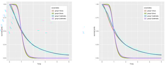
Figure 1. Predicted survival functions for the transformation models with crossed survival curves under random censoring (left) and fixed censoring (right).

7. Real Data Analysis

In this section, we apply our proposed method to the randomized AIDs clinical trial conducted in 1997 (recall from the introduction section). As stated previously, one major objective of this study was to examine treatment effects across different treatment groups through the plasma HIV-1 RNA level as the outcome variable, which is subject to double censoring. In the analysis, we create a variable $\mathrm{trt}$ which takes up the value 0 if a subject receives either Zidovudine(ZDV)+lamivudine(3TC) or stavudine(d4T)+ritonavir(RTV), and $\mathrm{trt}=1$ if a subject receives ZDV plus 3TC plus RTV. A remark should be made that this dataset was actually conducted under a fixed censoring scenario due to limitations of measuring techniques, resulting in the fact that all baseline log(RNA) levels could only be exactly observed between $-2.60$/mL and $5.88$/mL of plasma.

Below we present the analysis results of the proposed method along with the results from spBayesSurv and Li2018 methods, mainly for demonstration purposes. A visual aid is also provided for better distinction of treatment effects between the two treatment groups.

Based on the analysis of the AIDS clinical trial data, as shown in Table 6, the results consistently show that the triple therapy treatment group (ZDV + 3TC + RTV, trt = 1) had a significantly better outcome compared to the dual therapy groups (trt = 0), indicating lower HIV-1 RNA levels or higher survival probability. This finding is supported by all the methods tested (Proposed, spBayes PH/PO, Li2018 PH/PO), as their 95% credible/confidence intervals for the treatment effect (trt) were entirely positive and excluded zero. For example, the proposed method estimated a treatment effect of 1.057 (95% credible interval: 0.504 to 1.770).

Table 6. Results of AIDS study analysis.

	Proposed Method (Model (1))		Proposed Method (Model (7))
	trt	baseRNA	trt	baseRNA
Est	0.956	0.256	\	0.565
SD	0.050	0.150	\	0.159
95% CI	(0.826, 1.000)	(−0.009, 0.564)	\	(0.317, 0.836)
	spBayes PH		spBayes PO
	trt	baseRNA	trt	baseRNA
Est	1.058	0.245	1.437	0.382
SD	0.258	0.194	0.330	0.264
95% CI	(0.571, 1.583)	(−0.138, 0.623)	(0.803, 2.097)	(−0.141, 0.893)
	Li2018 PH r = 0		Li2018 PO r = 1
	trt	baseRNA	trt	baseRNA
Est	0.982	0.067	1.291	0.145
SD	0.272	0.180	0.308	0.261
95% CI	(0.449, 1.516)	(−0.285, 0.419)	(0.688, 1.894)	(−0.365, 0.656)

In contrast, without considering the heterogeneity of the categorical covariate, the effect of baseline RNA level (baseRNA) was not statistically significant in any analysis, indicating no strong evidence that the starting RNA level influenced the outcome. However, when we took into account the heterogeneity of the categorical variables, we found that the RNA level significantly influenced the outcome. Furthermore, the length of the credible interval provided by our two methods is much shorter than the others, indicating that the effect estimated by our method is more precise. Figure 2 visually confirms the main treatment effect that the lower survival probabilities for the dual therapy group compared to the triple therapy group over time.

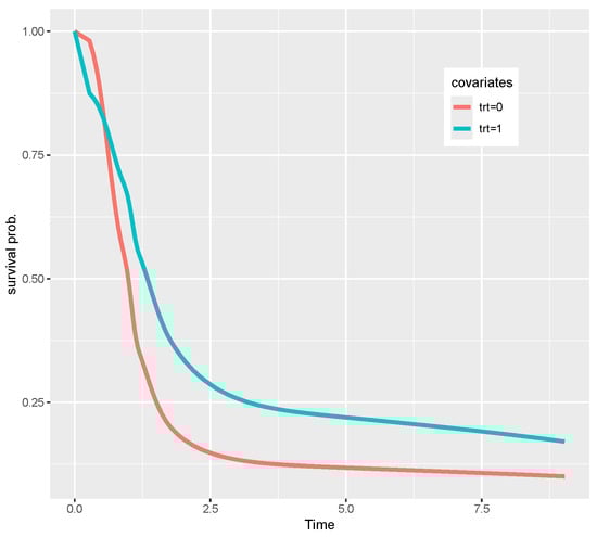
Figure 2. Predicted survival functions for the two treatment groups under Model (7).

8. Discussion

In this paper, we have proposed an innovative approach to analyze double-censored data and demonstrated its superior accuracy and flexibility over alternative methods. Namely, we bring up a new type of weakly informative prior, the pseudo-quantile I-splines priors, that allows for nonparametric estimation and prediction of double-censored time-to-event data under both random and fixed censoring schemes. We illustrate the effectiveness of this innovative prior by performing simulation results under several scenarios and comparing the proposed methods with two leading alternative methods. Our methodology can be treated as a robust survival analysis approach, as an alternative to the widely used Cox PH model.

For fixed censoring specifically, in addition to outperforming these methods considerably in some cases and displaying comparable results otherwise, our results are quite close to the assigned true values. This lends credibility to the statement that our method is not just the first to target estimation and prediction of double-censored time-to-events under fixed censoring, but also a valid method that deserves practical considerations. Subsequently, more attention should be paid to fixed censoring as a whole, since professionals who encounter such data can now be enabled with our proposed method or any future modification of it. We understand the complexity of fixed censoring and the intricacy around when only minimal information can be drawn from a substantial portion of observations. Despite these challenges, we believe that our approach of pseudo-data substitution has its merit, as the generated data may eventually mimic the true distribution of observations with minimally available information.

Our method enjoys robustness in predictions but sacrifices interpretability compared with semiparametric or parametric approaches. Here, we quote [33] (p. 559), “we should not confine ourselves to a hazard interpretation, especially when the hazards are not proportional and alternative formulations lead to more parsimonious models”. In this sense, our method supplies an alternative to those interpretable models in predictive inference. In our application example, on the one hand, when using the same homogeneous model, the significance of the treatment effect given by our method is consistent with other methods. On the other hand, when we incorporate the categorical heteroscedasticity, we reveal that the baseRNA is also significant. This finding demonstrates the utility of our method in the interpretation of the effect.

Our method employs MCMC under unidentified models, which demand heavier computational burden compared with those computed under identified models. It will be interesting to explore the approximate Bayesian computation (ABC) under the nonparametric transformation models. We leave this as our future work. Another interesting future work will be to relax the noninformative censoring assumption on the censoring scheme.

References

- Huang, J. Asymptotic properties of nonparametric estimation based on partly interval-censored data. Stat. Sin. 1999, 9, 501–519. [Google Scholar]
- Gao, F.; Zeng, D.; Lin, D.Y. Semiparametric estimation of the accelerated failure time model with partly interval-censored data. Biometrics 2017, 73, 1161–1168. [Google Scholar] [CrossRef] [PubMed]
- Gehan, E.A. A Generalized Two-Sample Wilcoxon Test for Doubly Censored Data. Biometrika 1965, 52, 650–653. [Google Scholar] [CrossRef] [PubMed]
- Ren, J.J.; Peer, P.G. A study on effectiveness of screening mammograms. Int. J. Epidemiol. 2000, 29, 803–806. [Google Scholar] [CrossRef] [PubMed]
- Jones, G.; Rocke, D.M. Multivariate survival analysis with doubly-censored data: Application to the assessment of Accutane treatment for fibrodysplasia ossificans progressiva. Stat. Med. 2002, 21, 2547–2562. [Google Scholar] [CrossRef]
- Cai, T.; Cheng, S. Semiparametric Regression Analysis for Doubly Censored Data. Biometrika 2004, 91, 277–290. [Google Scholar] [CrossRef]
- Sun, J. The Statistical Analysis of Interval-Censored Failure Time Data; Springer: New York, NY, USA, 2006. [Google Scholar]
- Turnbull, B.W. Nonparametric Estimation of a Survivorship Function with Doubly Censored Data. J. Am. Stat. Assoc. 1974, 69, 169–173. [Google Scholar] [CrossRef]
- Chang, M.N. Weak Convergence of a Self-Consistent Estimator of the Survival Function with Doubly Censored Data. Ann. Stat. 1990, 18, 391–404. [Google Scholar] [CrossRef]
- Gu, M.G.; Zhang, C.H. Asymptotic Properties of Self-Consistent Estimators Based on Doubly Censored Data. Ann. Stat. 1993, 21, 611–624. [Google Scholar] [CrossRef]
- Mykland, P.A.; Ren, J. Algorithms for Computing Self-Consistent and Maximum Likelihood Estimators with Doubly Censored Data. Ann. Stat. 1996, 24, 1740–1764. [Google Scholar] [CrossRef]
- Zhang, Y.; Jamshidian, M. On algorithms for the nonparametric maximum likelihood estimator of the failure function with censored data. J. Comput. Graph. Stat. 2004, 13, 123–140. [Google Scholar] [CrossRef]
- Cox, D.R. Regression models and life-tables. J. R. Stat. Soc. Ser. B 1972, 34, 187–202. [Google Scholar] [CrossRef]
- Kim, Y.; Kim, B.; Jang, W. Asymptotic properties of the maximum likelihood estimator for the proportional hazards model with doubly censored data. J. Multivar. Anal. 2010, 101, 1339–1351. [Google Scholar] [CrossRef]
- Kim, Y.; Kim, J.; Jang, W. An EM algorithm for the proportional hazards model with doubly censored data. Comput. Stat. Data Anal. 2013, 57, 41–51. [Google Scholar] [CrossRef]
- Cheng, S.; Wei, L.; Ying, Z. Analysis of transformation models with censored data. Biometrika 1995, 82, 835–845. [Google Scholar] [CrossRef]
- Chen, K.; Jin, Z.; Ying, Z. Semiparametric analysis of transformation models with censored data. Biometrika 2002, 89, 659–668. [Google Scholar] [CrossRef]
- Zeng, D.; Lin, D. Efficient estimation of semiparametric transformation models for counting processes. Biometrika 2006, 93, 627–640. [Google Scholar] [CrossRef]
- de Castro, M.; Chen, M.H.; Ibrahim, J.G.; Klein, J.P. Bayesian transformation models for multivariate survival data. Scand. J. Stat. 2014, 41, 187–199. [Google Scholar] [CrossRef]
- Li, S.; Hu, T.; Wang, P.; Sun, J. A Class of Semiparametric Transformation Models for Doubly Censored Failure Time Data. Scand. J. Stat. 2018, 45, 682–698. [Google Scholar] [CrossRef]
- Hothorn, T.; Kneib, T.; Bühlmann, P. Conditional transformation models. J. R. Stat. Soc. Ser. B Stat. Methodol. 2014, 76, 3–27. [Google Scholar] [CrossRef]
- Hothorn, T.; Möst, L.; Bühlmann, P. Most likely transformations. Scand. J. Stat. 2018, 45, 110–134. [Google Scholar] [CrossRef]
- Zhou, H.; Hanson, T. A unified framework for fitting Bayesian semiparametric models to arbitrarily censored survival data, including spatially referenced data. J. Am. Stat. Assoc. 2018, 113, 571–581. [Google Scholar] [CrossRef]
- Kowal, D.R.; Wu, B. Monte Carlo inference for semiparametric Bayesian regression. J. Am. Stat. Assoc. 2024, 120, 1063–1076. [Google Scholar] [CrossRef] [PubMed]
- Zhong, C.; Yang, J.; Shen, J.; Liu, C.; Li, Z. On MCMC mixing under unidentified nonparametric models with an application to survival predictions under transformation models. arXiv 2024, arXiv:2411.01382. [Google Scholar] [CrossRef]
- Horowitz, J.L. Semiparametric estimation of a regression model with an unknown transformation of the dependent variable. Econometrica 1996, 64, 103–137. [Google Scholar] [CrossRef]
- Ye, J.; Duan, N. Nonparametric n−1/2-consistent estimation for the general transformation models. Ann. Stat. 1997, 25, 2682–2717. [Google Scholar] [CrossRef]
- Chen, S. Rank Estimation of Transformation Models. Econometrica 2002, 70, 1683–1697. [Google Scholar] [CrossRef]
- Mallick, B.K.; Walker, S. A Bayesian semiparametric transformation model incorporating frailties. J. Stat. Plan. Inference 2003, 112, 159–174. [Google Scholar] [CrossRef]
- Song, X.; Ma, S.; Huang, J.; Zhou, X.H. A semiparametric approach for the nonparametric transformation survival model with multiple covariates. Biostatistics 2007, 8, 197–211. [Google Scholar] [CrossRef]
- Cuzick, J. Rank regression. Ann. Stat. 1988, 16, 1369–1389. [Google Scholar] [CrossRef]
- Gørgens, T.; Horowitz, J.L. Semiparametric estimation of a censored regression model with an unknown transformation of the dependent variable. J. Econom. 1999, 90, 155–191. [Google Scholar] [CrossRef]
- Zeng, D.; Lin, D. Efficient estimation for the accelerated failure time model. J. Am. Stat. Assoc. 2007, 102, 1387–1396. [Google Scholar] [CrossRef]
- Ramsay, J.O. Monotone regression splines in action. Stat. Sci. 1988, 3, 425–441. [Google Scholar] [CrossRef]
- MacEachern, S.N. Dependent Nonparametric Processes. In Proceedings of the Section on Bayesian Statistical Science; American Statistical Association: Alexandria, VA, USA, 1999. [Google Scholar]
- De Iorio, M.; Müller, P.; Rosner, G.L.; MacEachern, S.N. An ANOVA model for dependent random measures. J. Am. Stat. Assoc. 2004, 99, 205–215. [Google Scholar] [CrossRef]
- Lo, A.Y. On a class of Bayesian nonparametric estimates: I. Density estimates. Ann. Stat. 1984, 12, 351–357. [Google Scholar] [CrossRef]
- Sethuraman, J. A constructive definition of Dirichlet priors. Stat. Sin. 1994, 4, 639–650. [Google Scholar]
- Kottas, A. Nonparametric Bayesian survival analysis using mixtures of Weibull distributions. J. Stat. Plan. Inference 2006, 136, 578–596. [Google Scholar] [CrossRef]
- Gelman, A.; Carlin, J.B.; Stern, H.S.; Dunson, D.B.; Vehtari, A.; Rubin, D.B. Bayesian Data Analysis; CRC Press: Boca Raton, FL, USA, 2013. [Google Scholar]
- Ishwaran, H.; James, L.F. Approximate Dirichlet process computing in finite normal mixtures: Smoothing and prior information. J. Comput. Graph. Stat. 2002, 11, 508–532. [Google Scholar] [CrossRef]
- Zhong, C.; Ma, Z.; Shen, J.; Liu, C. Dependent Dirichlet Processes for Analysis of a Generalized Shared Frailty Model. In Computational Statistics and Applications; Løpez-Ruiz, R., Ed.; Chapter 5; IntechOpen: Rijeka, Croatia, 2021. [Google Scholar]
- Carpenter, B.; Gelman, A.; Hoffman, M.D.; Lee, D.; Goodrich, B.; Betancourt, M.; Brubaker, M.A.; Guo, J.; Li, P.; Riddell, A. Stan: A probabilistic programming language. J. Stat. Softw. 2017, 76, 1–32. [Google Scholar] [CrossRef]
- Absil, P.A.; Malick, J. Projection-like retractions on matrix manifolds. SIAM J. Optim. 2012, 22, 135–158. [Google Scholar] [CrossRef]
Disclaimer/Publisher’s Note: The statements, opinions and data contained in all publications are solely those of the individual author(s) and contributor(s) and not of MDPI and/or the editor(s). MDPI and/or the editor(s) disclaim responsibility for any injury to people or property resulting from any ideas, methods, instructions or products referred to in the content. |
© 2025 by the authors. Licensee MDPI, Basel, Switzerland. This article is an open access article distributed under the terms and conditions of the Creative Commons Attribution (CC BY) license (https://creativecommons.org/licenses/by/4.0/).