Enhanced Temporal Action Localization with Separated Bidirectional Mamba and Boundary Correction Strategy

Abstract

Temporal action localization (TAL) is a research hotspot in video understanding, which aims to locate and classify actions in videos. However, existing methods have difficulties in capturing long-term actions due to focusing on local temporal information, which leads to poor performance in localizing long-term temporal sequences. In addition, most methods ignore the boundary importance for action instances, resulting in inaccurate localized boundaries. To address these issues, this paper proposes a state space model for temporal action localization, called Separated Bidirectional Mamba (SBM), which innovatively understands frame changes from the perspective of state transformation. It adapts to different sequence lengths and incorporates state information from the forward and backward for each frame through forward Mamba and backward Mamba to obtain more comprehensive action representations, enhancing modeling capabilities for long-term temporal sequences. Moreover, this paper designs a Boundary Correction Strategy (BCS). It calculates the contribution of each frame to action instances based on the pre-localized results, then adjusts weights of frames in boundary regression to ensure the boundaries are shifted towards the frames with higher contributions, leading to more accurate boundaries. To demonstrate the effectiveness of the proposed method, this paper reports mean Average Precision (mAP) under temporal Intersection over Union (tIoU) thresholds on four challenging benchmarks: THUMOS13, ActivityNet-1.3, HACS, and FineAction, where the proposed method achieves mAPs of 73.7%, 42.0%, 45.2%, and 29.1%, respectively, surpassing the state-of-the-art approaches.

1. Introduction

Temporal action localization (TAL) is a challenging but crucial task in understanding videos, and it has gained significant interest over the past few years. TAL requires the localization and classification of all action instances within an untrimmed video. Localization aims to accurately determine the temporal boundaries of action instances, while classification identifies the corresponding action categories. Compared with other video-understanding tasks, TAL accurately determines the duration and category of the action in the untrimmed video. Therefore, TAL is widely adopted in action retrieval, intelligent surveillance, and human movement analysis [1,2,3,4].

As deep learning continues to develop, many TAL methods based on deep learning have emerged [5]. These methods first employ pre-extracted features as inputs of the deep neural network, including I3D [6], SlowFast [7], and VideoMAEv2 [8]. Then, the encoder, called backbone, performs contextual modeling of the features. Finally, the decoder classifies the actions and estimates the corresponding boundaries.

Recently, Transformer [9] has become popular due to its successful application in understanding videos [10]. To extract intrinsic information from actions, many methods [11,12,13,14,15,16,17] introduce Transformer and its improved methods into TAL, which capture long-term temporal dependencies between frames, facilitating the localization and classification of long-term actions. Subsequently, several methods [8,18,19] realize a problem in the self-attention of Transformer, which is that obtained features are highly similar but difficult to distinguish. Thus, they follow the basic architecture of Transformer-based methods and replace self-attention with other forms of convolutional neural networks (CNNs), bringing further performance improvements.

In fact, these solutions [8,18,19] still have drawbacks. For example, the local perception of CNNs hinders the model from effectively utilizing the global information, which brings a challenge for temporal localization of long-term actions. In addition, many TAL methods [8,11,18] ignore the boundary importance for action instances, resulting in inaccurate localized boundaries. Specifically, if the model gives higher regression weights to frames that are farther away from the ground-truth, the predictions tend to have larger errors. It is detrimental for models to accurately capture action instances.

Therefore, a state space model (SSM) for TAL, called Separated Bidirectional Mamba (SBM), is proposed. Based on the continuity of frames, SBM understands the changes between neighboring frames as state transformation. Specifically, it involves a set of unidirectional Mamba, which fuses filtered forward and backward state information, generating temporal features that cover global context information. This effectively improves the model’s ability to model long-term temporal sequences. Inspired by these methods [2,20], the Boundary Correction Strategy (BCS) is innovatively designed, which evaluates the contribution of each frame to action instances based on its action sensitivity. Guided by these contributions, the model corrects the pre-localized boundaries to make them more accurate.

The primary contributions of this paper are summed up as follows:

• This paper proposes SBM, which consists of a set of unidirectional Mamba that brings forward and backward information to frames from the perspective of state transformation. It fully utilizes the global forward and backward temporal information, which improves the model’s capacity for modeling long-term temporal sequences.
• In this paper, BCS is designed to obtain the contribution of each frame to action instances by utilizing its action sensitivity and directs these contributions toward refining boundaries. It distinguishes frames near the ground-truth boundaries from other frames in a video, resulting in more accurately predicted boundaries.
• Experimental results indicate that the proposed method has a better performance than the state-of-the-art (SOTA) methods, thus demonstrating its superiority and effectiveness. In addition, this paper promotes the application of SSMs in TAL.

The remainder of this paper is structured as follows: Section 2 reviews related works. Section 3 describes the overall framework and implementation details of the proposed method, including SBM and BCS. Section 4 shows and analyzes the experimental results. Section 5 concludes this paper and presents future work.

2. Related Work

2.1. Temporal Action Localization (TAL)

TAL is a hot research topic in video understanding, which focuses on the localization and classification of actions in uncropped videos. Currently, the mainstream TAL methods directly perform frame-level classification and boundary regression. Due to its automation and low complexity, it has gained significant interest over the past few years. Lin et al. [21] propose the first purely anchorless TAL method that finds accurate boundaries even given an arbitrary proposal. Similarly, Yang et al. [22] present an anchorless action localization module that assists action localization through time points. Lin et al. [23] introduce a 1D temporal convolutional layer-based approach for TAL, which directly detects action instances in untrimmed videos without relying on proposal generation.

In recent years, Transformer [9] has been widely used in video understanding. Inspired by this, Zhang et al. [11] construct a Transformer-based TAL framework that integrates multi-scale feature representation with local self-attention and applies a lightweight decoder to determine action instances. Tang et al. [18] follow the basic architecture of the method in reference [11] but use simple max-pooling instead of the Transformer encoder to minimize redundancy and accelerate training. Shi et al. [8] replace self-attention with a scalable granularity perception layer and design a Trident-head for modeling boundaries by estimating relative probability distributions around boundaries. Li et al. [13] propose an innovative Transformer for TAL that adaptively integrates feature representations from different attention heads. Furthermore, Yang et al. [19] propose an effective fusion strategy, which dynamically adjusts the receptive field at different timesteps to aggregate the temporal features within the action intervals.

2.2. State Space Models (SSMs)

SSM-based methods have emerged in recent years, since SSMs bring together the strengths of multiple sequence model design paradigms. Gu et al. [24] introduce a new SSM, which parameterizes the state matrix by a diagonal plus low-rank structure for high-performance computation. At the same time, this model provides a new way to model long-term temporal sequences. Smith et al. [25] further propose a simplified SSM for sequence modeling, which utilizes a multiple-input and multiple-output SSM to achieve efficient parallel scanning. Gupta et al. [26] design diagonal SSMs that contain only diagonal state matrices and achieves comparable performance to the method in reference [24]. Fu et al. [27] design a new SSM layer that achieves a performance matching Transformer in terms of languages synthesis. However, the constant sequence transformation of SSMs limits their context-based inference capability, which hinders their further development in long-term temporal sequence modeling.

Recently, Gu et al. [28] propose Mamba, which lets the model choose to transmit or discard information along the sequence for the current token and designs a hardware-aware parallel algorithm that brings fast inference with linear complexity. With the increasing integration of Natural Language Processing techniques into video understanding, the application of Mamba is becoming more prevalent. Liu et al. [29] design a set of visual state space blocks with the 2D selective scanning module that allows the model to better adapt to the non-sequential structure of 2D visual data. Similarly, Yang et al. [30] propose a basic non-hierarchical SSM, which enhances its ability to learn visual features through a sequential 2D scanning process and enables the model to discriminate the spatial relationships of tokens through direction-aware updating. Zhu et al. [31] design a network with bidirectional Mamba blocks. This network uses position embedding to mark the image sequence and compresses feature representations using a bidirectional SSM. Li et al. [32] design a generic module for extending the Mamba architecture to arbitrary multidimensional data.

3. Method

Given a set of uncropped videos, the TAL model first extracts the temporal features $xϵR^{D\times T}$ of each video using a visual backbone network, where D and T are the number of channels and frames. Then, it predicts a series of possible action instances $\mathrm{\Psi }={\{{\psi }_m=(t_m^s,t_m^e,c_m)\}}_{m=1}^M$, where M presents the number of predicted results for this video, and $t_m^s$, $t_m^e$ and $c_m$ denote the boundary and action category of the m-th predicted result, respectively. It is summarized as

$$\mathrm{\Psi }=TLoc\left(x\right)$$

(1)

3.1. Framework Overview

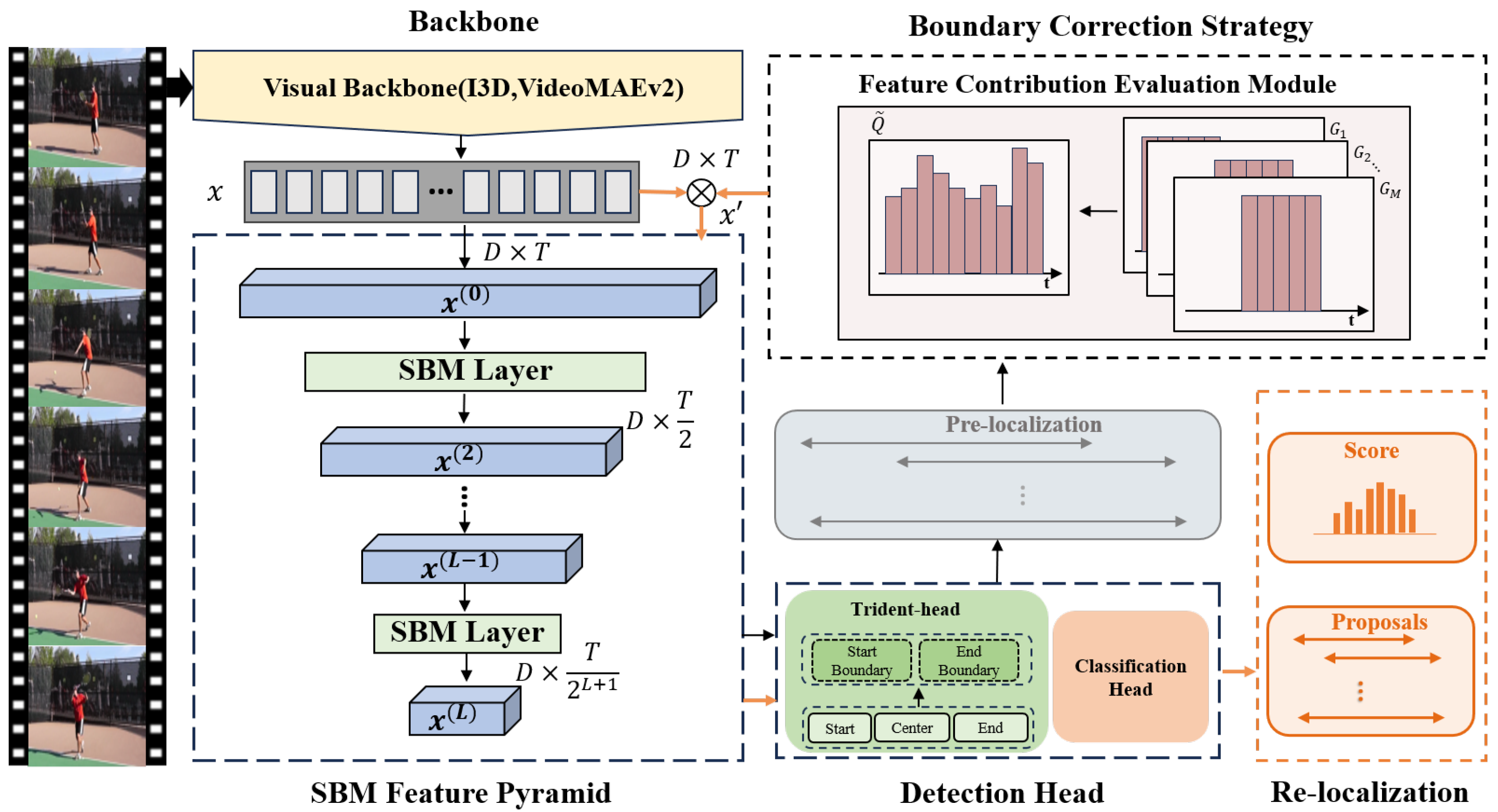
The overall framework is shown in Figure 1, which includes four components: visual backbone network, SBM feature pyramid, detection head, and BCS.

First, the model extracts temporal features using a visual backbone network, and the SBM feature pyramid encodes them into multi-scale temporal features containing global context information. Next, the detection head performs frame-level localization and classification to generate pre-localized results.

Next, BCS determines the action sensitivity of frames based on the pre-localized results and then generates the contribution of each frame to the action instance. The contribution is adopted for the weighted aggregation of temporal features, to boost the response values of frames near boundaries and suppress others, which makes the predicted boundaries more accurate.

Lastly, the updated features are fed sequentially into the SBM feature pyramid to obtain the re-localized results.

The SBM feature pyramid and BCS are described in Section 3.2 and Section 3.3, and Section 3.4 exhibits a time complexity analysis of the proposed method.

3.2. The SBM Feature Pyramid

Current TAL methods replace the Transformer encoder with CNNs to tackle the problems of feature redundancy and rank loss caused by self-attention. However, these methods still have shortcomings. For example, it has difficulty in dealing with long-term temporal sequences, due to the limitation in capturing global time information.

Recently, SSMs have been introduced into deep learning for sequence modeling. Their main idea is applying hidden states to connect input and output sequences, essentially a sequence transformation. Unlike the local modeling of CNNs, SSMs provide a more comprehensive data description through explicit hidden states and transformation equations.

Therefore, this paper designs an SBM feature pyramid. It applies hidden states to provide forward and backward information for frames, which helps the model understand the changes between frames. Specifically, the SBM feature pyramid consists of multiple sequentially connected SBM layers, which pass the temporal features obtained from one layer to the next for encoding, thus obtaining multi-scale temporal features.

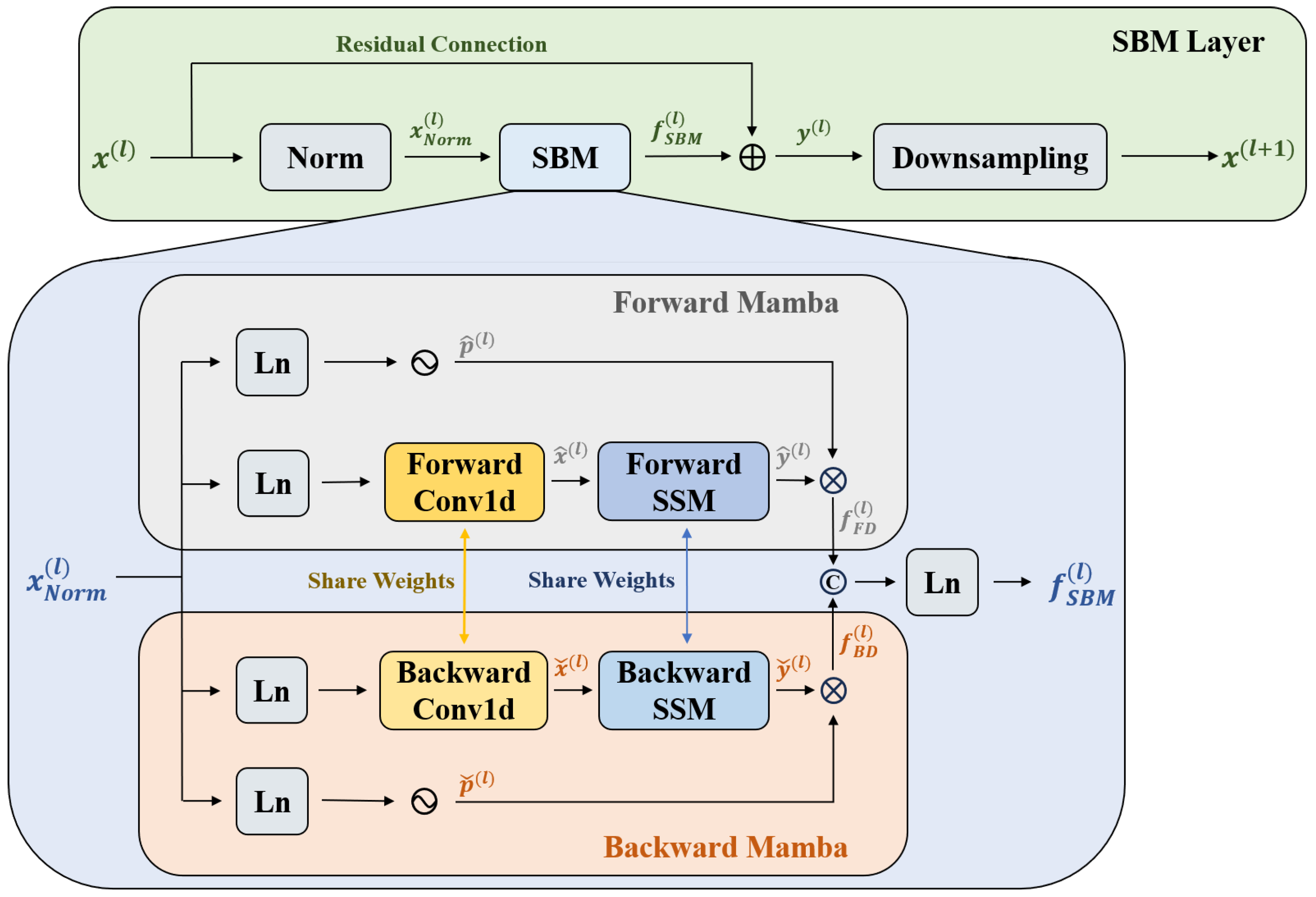
Figure 2 depicts the SBM layer, which is separated into main and branch paths. The main path contains a normalization module and an SBM module for aggregating global context information and a down-sampling layer for constructing the feature pyramid. The branch path is a residual connection, which connects the input directly to the main output to minimize original information loss. The normalization process is represented by

$$x_{Norm}^{\left(l\right)}=Norm\left(x^{\left(l\right)}\right)$$

(2)

where $Norm(•)$ denotes the layer normalization operation, $x_{Norm}^{\left(l\right)}$ is the input temporal feature of the l-th SBM layer, and $x^{\left(0\right)}$ is the initial temporal feature x.

Formally, the SBM contains two components: the forward and backward Mamba, which are applied to incorporate forward and backward contextual information for temporal features.

Forward Mamba: The gate-modeling branch produces the temporal feature ${\overrightarrow{y}}^{\left(l\right)}$ that incorporates the forward information. The above process is summarized as

$$\begin{array}{c}{\overrightarrow{p}}^{\left(l\right)}=\sigma (Ln\left(x_{Norm}^{\left(l\right)}\right))\end{array}$$

(3)

$$\begin{array}{c}{\overrightarrow{x}}^{\left(l\right)}={Conv1d}_{FD}(Ln\left(x_{Norm}^{\left(l\right)}\right))\end{array}$$

(4)

$$\begin{array}{c}{\overrightarrow{y}}^{\left(l\right)}{=SSM}_{FD}\left({\overrightarrow{x}}^{\left(l\right)}\right)\end{array}$$

(5)

where $\sigma (•)$ presents the gate function, and the SiLU function is adopted in this paper. $Ln(•)$ is the linear layer. ${Conv1d}_{FD}$ refers to the forward 1D convolution. ${SSM}_{FD}$ is the forward SSM.

${SSM}_{FD}$ is presented to convert the input ${\left\{{\overrightarrow{x}}_t^{\left(l\right)}\right\}}_{t=1}^T$ to the output $\left\{{\overrightarrow{y}}_t^{\left(l\right)}\right\}{)}_{t=1}^T$. Specifically, it converts the last hidden state ${\overrightarrow{h}}_{t-1}^{\left(l\right)}$ and the present input ${\overrightarrow{x}}_t^{\left(l\right)}$ into the present hidden state ${\overrightarrow{h}}_t^{\left(l\right)}$, then transfers ${\overrightarrow{h}}_t^{\left(l\right)}$ to the present output ${\overrightarrow{y}}_t^{\left(l\right)}$. This conversion is formulated as

$$\begin{array}{c}{\overrightarrow{h}}_t^{\left(l\right)}=\overline{A}{\overrightarrow{h}}_{t-1}^{\left(l\right)}+\overline{B}{\overrightarrow{x}}_t^{\left(l\right)}\end{array}$$

(6)

$$\begin{array}{c}{\overrightarrow{y}}_t^{\left(l\right)}=C{\overrightarrow{h}}_t^{\left(l\right)}\end{array}$$

(7)

where matrices $\overline{A}\in {\mathbb{R}}^{B\times T\times D\times N}$, $\overline{B}\in {\mathbb{R}}^{B\times T\times D\times N}$, and $C\in {\mathbb{R}}^{B\times T\times N}$ are trainable parameters of ${SSM}_{FD}$. B represents batch size, N is the state size, and T and D are the number of frames and channels. Both $\overline{A}$ and $\overline{B}$ are discretized. $\overline{A}$ and $\overline{B}$ define the evolution of hidden states, and C projects hidden states to outputs. The initial hidden state ${\overrightarrow{h}}_0^{\left(l\right)}$ is defined as a zero vector.

Finally, ${\overrightarrow{p}}^{\left(l\right)}$ and ${\overrightarrow{y}}^{\left(l\right)}$ are multiplied to obtain the forward Mamba result $f_{FD}^{\left(l\right)}$ to emphasize the key information and reduce the influence of secondary information, which is formulated as

$$f_{FD}^{\left(l\right)}={\overrightarrow{p}}^{\left(l\right)}\otimes {\overrightarrow{y}}^{\left(l\right)}$$

(8)

Backward Mamba: To fuse the bidirectional features, this method further defines the backward Mamba. It incorporates backward information in temporal features, thus complementing details and patterns that tend to be missed by forward information. Similarly to forward Mamba, the computational process for backward Mamba is represented by

$$\begin{array}{c}{\overleftarrow{p}}^{\left(l\right)}=\sigma (Ln(x_{Norm}^{\left(l\right)}))\end{array}$$

(9)

$$\begin{array}{c}{\overleftarrow{x}}^{\left(l\right)}={Conv1d}_{BD}(Ln(x_{Norm}^{\left(l\right)}))\end{array}$$

(10)

$$\begin{array}{c}{\overleftarrow{y}}^{\left(l\right)}{=SSM}_{BD}({\overleftarrow{x}}^{\left(l\right)})\end{array}$$

(11)

where ${Conv1d}_{BD}$ denotes the backward 1D convolution, sharing weights with ${Conv1d}_{FD}$, and ${SSM}_{BD}$ is the backward SSM, sharing weights with ${SSM}_{FD}$.

Finally, ${\overleftarrow{p}}^{\left(l\right)}$ and ${\overleftarrow{y}}^{\left(l\right)}$ are multiplied to obtain the backward Mamba output $f_{BD}^{\left(l\right)}$ as shown in

$$f_{BD}^{\left(l\right)}={\overleftarrow{p}}^{\left(l\right)}\otimes {\overleftarrow{y}}^{\left(l\right)}$$

(12)

SBM concatenates $f_{FD}^{\left(l\right)}$ with $f_{BD}^{\left(l\right)}$ and then obtains the final result through the linear layer. This operation is defined as

$$f_{SBM}^{\left(l\right)}=Ln(Concat(f_{FD}^{\left(l\right)},f_{BD}^{\left(l\right)}))$$

(13)

Through the above steps, the SBM layer realizes the encoding of temporal features at each scale and obtains the temporal feature $y^{\left(l\right)}$ that incorporates the global context information. The overall process is summarized in

$$y^{\left(l\right)}=f_{SBM}^{\left(l\right)}+x^{\left(l\right)}$$

(14)

Finally, $y^{\left(l\right)}$ enters the down-sampling layer to obtain the input of the next SBM layer, as shown in

$$x^{(l+1)}=DS\left(y^{\left(l\right)}\right)$$

(15)

where $DS(•)$ denotes the maximum pooling layer.

3.3. Boundary Correction Strategy (BCS)

In TAL, not every frame contributes equally. In terms of the boundary regression task, frames distant from the ground-truth boundaries often lead to boundary offset errors, making predicted boundaries large biases, which reduces the localization accuracy.

Therefore, BCS calculates the frame contribution based on the pre-localized result, and then uses it for feature updating, which corrects boundaries for refined-local results. Formally, it divides the TAL into the pre-localized and the boundary refinement stage.

Pre-localized Stage: In the pre-localized stage, this paper follows the Trident-head [7] for boundary regression. Trident-head includes start header, end header and center offset header, which determine boundaries, and action centers, respectively.

For an arbitrary scale temporal feature $Xϵ{\left\{x^{\left(l\right)}\right\}}_{l=0}^L$, it is first encoded into three features: $I^sϵR^T$, $I^eϵR^T$, and $I^oϵR^{T\times 2\times (B+1)}$, where $I^s$ and $I^e$ denote each frame response value as a start and end boundary, respectively, and $I^o$ denotes its relative center offsets. The coding process is expressed as

$$I^s,I^e,I^o=\mathcal{F}\left(X\right)$$

(16)

where $\mathcal{F}(•)$ denotes the process of encoding.

Then, this paper estimates the distance probability distribution from the start boundary to the action center, with the start response value and the relative center offsets. For example, when frame i is the action center, the distance probability distribution $P\left(d_i^s=b\right)$ of the distance $d_i^s$ between the start boundary and the action center is shown in Equation (17). Moreover, $b=0,1,\dots ,B$, B denotes the predefined maximum distance between the start boundary and the action center.

$$P(d_i^s=b)=\phi (I_{i-b}^s+I_{i,0,b}^o)$$

(17)

where $I_{i-b}^s$ represents the response value (the b-th frame to the left of frame i is the start boundary), and $I_{i,0,b}^o$ denotes its relative center offsets.

Based on the above probability distribution, this paper approximates the start boundary $t_i^s$ by calculating the expectation $E\left[d_i^s\right]$, as shown in

$$\begin{array}{c}E\left[d_i^s\right]=\sum _{b=0}^{B}bP(d_i^s=b)\end{array}$$

(18)

$$\begin{array}{c}{t}_i^s=(i-E\left[d_i^s\right])\times {\delta }^{l-1}\end{array}$$

(19)

where $\delta$ is the down-sampling rate.

Similarly, when the i-th frame is the action center, the end boundary $t_i^s$ is received by

$$\begin{array}{c}P(d_i^e=b)=\phi (I_{i+b}^e+I_{i,1,b}^o)\end{array}$$

(20)

$$\begin{array}{c}E\left[d_i^e\right]=\sum _{b=0}^{B}bP(d_i^e=b)\end{array}$$

(21)

$$\begin{array}{c}{t}_i^e=(i+E\left[d_i^e\right])\times {\delta }^{l-1}\end{array}$$

(22)

where $d_i^e$ denotes the distance from the end boundary to the action center. $I_{i+b}^e$ represents the response value (the b-th frame to the action center right is the end boundary), and $I_{i,1,b}^o$ is its relative center offsets.

Then, the action instance ${\psi }_i=(t_i^s,t_i^e,c_i)$ is given after merging the action boundary with the action category. The action category is obtained from

$$c_i=Cls\left(X_i\right)$$

(23)

where $Cls(•)$ is the classification head.

Finally, a non-maximal suppression operation is applied to filter the redundant action instances to obtain pre-localized result $\mathrm{\Psi }={\{{\psi }_m=(t_m^s,t_m^e,c_m)\}}_{m=1}^M$, which is expressed by

$$\mathrm{\Psi }\leftarrow \left\{NMS\left({\psi }_i\right)\right|{Conf}_{{\psi }_i}>\lambda \}$$

(24)

where $NMS(•)$ is a non-maximal suppression operation. ${Conf}_{{\psi }_i}$ denotes the confidence of the action instance ${\psi }_i$. $\lambda$ is the confidence threshold.

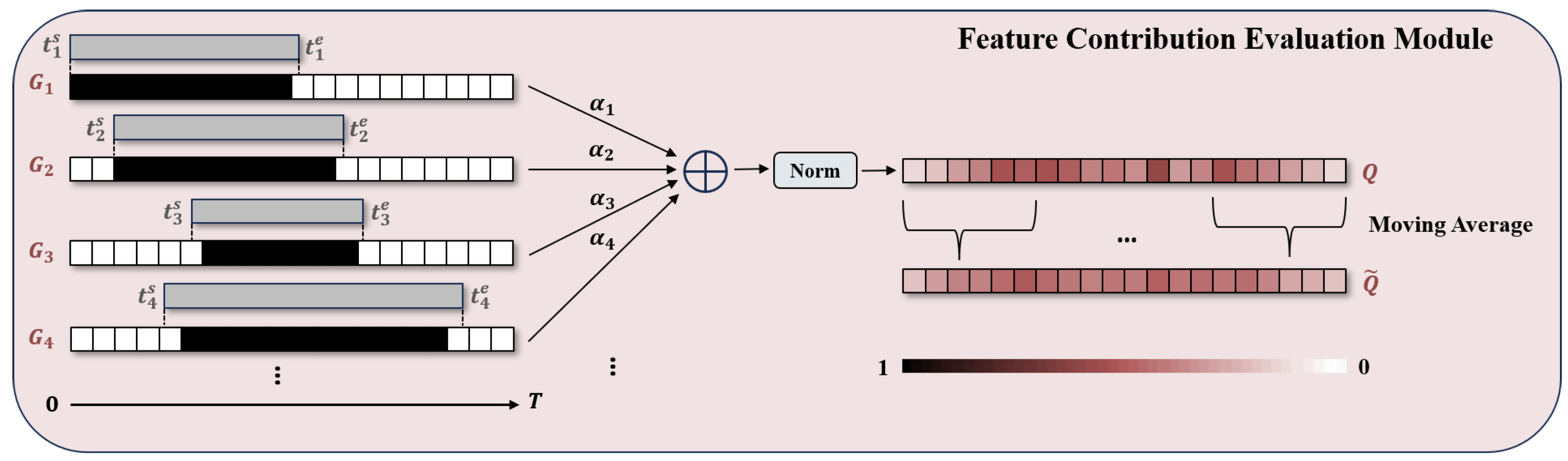
Boundary Refinement Stage: The boundary refinement stage uses the Feature Contribution Evaluation Module (FCEM) to quantify the action sensitivity of each frame and then gives it a contribution score. The FCEM is shown in Figure 3.

First, FCEM calculates the action sensitivity for each frame based on the action instance $\mathrm{\Psi }$. Specifically, FCEM stacks each action instance with the timeline chronologically, assigning nonzero action sensitivity to the overlapping portion of frames. The frame sensitivity $G_m$ is calculated using

$$\begin{array}{cc}\hfill G_m& ={\left({score}_t\right)}_{t=1}^T\hfill \\ \hfill scor{e}_t& =\left\{\begin{array}{c}\gamma ,t\in [t_m^s,t_m^e]\hfill \\ 0,else\hfill \end{array}\right.\hfill \end{array}$$

(25)

where $\gamma$ is a nonzero number.

Frame sensitivity reflects the degree sensitive of the frame to each action instance. In fact, a frame often exists in multiple pre-localized action instances, and the more a frame is located near the action boundary, the higher possibility of it appearing in an action instance. Therefore, to fully utilize the information of all action instances for frames, FCEM gets the frame contribution Q by fusing frame sensitivities $G_m$ as each frame importance in TAL. The process is summarized in

$$Q=Norm(\sum _{m=1}^M{\alpha }_m{G}_m)$$

(26)

where ${\alpha }_m$ presents the weight of $G_m$ in the fusion process, and $Norm(•)$ is the normalization process.

In addition, to improve the smoothness of the contribution matrix, FCEM also performs Moving Average (MA) on Q, which fuses the information of neighboring frames to reduce the sharp variations in data caused by noise. The frame contribution $\tilde{Q}$ is obtained using

$$\tilde{Q}=MA\left(Q\right)$$

(27)

Based on the frame contribution $\tilde{Q}$, BCS generates the updated temporal feature $x^{\prime }$, and the calculation process is shown in

$$x^{\prime }=x\otimes \tilde{Q}\ast \epsilon$$

(28)

where $\epsilon$ is the balance factor.

Finally, $x^{\prime }$ performs action localization based on Equations (2)–(24), to obtain the corrected action instances ${\mathrm{\Psi }}^{\prime }={\{{\psi }_m^{\prime }=({t_m^s}^{\prime },{t_m^e}^{\prime },c_m^{\prime })\}}_{m=1}^M$.

3.4. Time Complexity Analysis

First, the detailed processing of the SBM feature pyramid is represented by Algorithm 1.

Algorithm 1. The process of the SBM feature pyramid

Input:  Temporal feature x. Output:  Encoded features ${\left\{x^{\left(l\right)}\right\}}_{l=0}^L$. 1: $x^{\left(0\right)}\leftarrow x$ 2: /* Construct SBM feature pyramid */ 3: for l in {0,1,…,L-1} do 4:     $x_{Norm}^{\left(l\right)}\leftarrow Norm\left(x^{\left(l\right)}\right)$ 5:     /* SBM */ 6:     $f_{FD}^{\left(l\right)}\leftarrow FowardMamba(A,B,C,x_{Norm}^{\left(l\right)})$ 7:     $f_{BD}^{\left(l\right)}\leftarrow BackwardMamba(A,B,C,x_{Norm}^{\left(l\right)})$ 8:     $f_{SBM}^{\left(l\right)}\leftarrow Ln(Concat(f_{FD}^{\left(l\right)},f_{BD}^{\left(l\right)}))$ 9:     $y^{\left(l\right)}\leftarrow f_{SBM}^{\left(l\right)}+x^{\left(l\right)}$ 10:     $x^{(l+1)}\leftarrow DS\left(y^{\left(l\right)}\right)$ 11: end for 12: return ${\left\{x^{\left(l\right)}\right\}}_{l=0}^L$

Here, the time complexity is calculated as follows:

Since each SBM block incurs a time cost that is linear in its input sequence length [28], the pyramid halves that length at every layer. The 0-th layer processes the original T frames in $O\left(T\right)$ time, the 1-st layer processes ${\displaystyle \frac{T}{2}}$ frames in $O({\displaystyle \frac{T}{2}})$ time, and this pattern continues until the $(L-1)$-th layer takes $O({\displaystyle \frac{T}{2^{L-1}}})$ time. Summing the costs of all L layers yields $T_{\mathrm{total}}\left(T\right)={\sum }_{l=0}^{L-1}O({\displaystyle \frac{T}{2^l}})=O\left((2-{\displaystyle \frac{1}{2^{L-1}}})T\right)$. Because the bracketed factor is a bounded constant, the overall complexity remains $O\left(T\right)$, which is markedly better than the $O\left(T^2\right)$ complexity of Transformer.

Then, the detailed processing of BCS is represented by Algorithm 2.

Algorithm 2. BCS process

Input:  Temporal feature x. Output:  Corrected action instances ${\mathrm{\Psi }}^{\prime }$. 1: /* Pre-localized stage */ 2: ${\left\{x^{\left(l\right)}\right\}}_{l=0}^L\leftarrow SBM\left(x\right)$ 3: $\mathrm{\Psi }\leftarrow detectionhead\left({\left\{x^{\left(l\right)}\right\}}_{l=0}^L\right)$ 4: /* Boundary refinement stage */ >5: /* FCEM */ 6: for m in {1,2,…,M} do 7:     for t in {1,2,…,T} do 8:         if $t\ge t_m^s$ and $t\le t_m^e$ then 9:            ${score}_t\leftarrow \gamma$ 10:         else 11:            ${score}_t\leftarrow 0$ 12:         end if 13:     end for 14:     $G_m\leftarrow {\left\{\left({score}_t\right)\right\}}_{t=1}^T$ 15: end for 16: $Q\leftarrow Norm\left({\sum }_{m=1}^M{\alpha }_m{G}_m\right)$ 17: $\tilde{Q}\leftarrow MA\left(Q\right)$ 18: $x^{\prime }\leftarrow x\otimes \tilde{Q}\ast \epsilon$ 19: ${\mathrm{\Psi }}^{\prime }\leftarrow detectionhead\left({\left\{{x^{\left(l\right)}}^{\prime }\right\}}_{l=0}^L\right)$ 20: return ${\mathrm{\Psi }}^{\prime }$

The time consumption of BCS comes mainly from FCEM, which has to traverse each instance and each timestamp sequentially. Thus, its time complexity is $O\left(MT\right)$. Since M is generally less than T, it could be considered as linear time complexity.

Overall, with the time complexity of the detection head $O((2-{\displaystyle \frac{1}{2^L}})T)$, the total time complexity of the proposed method is approximately $O((4-{\displaystyle \frac{3}{2^L}}+M)T)$, which could be considered as linear time complexity $O\left(T\right)$. Therefore, compared to the Transformer-based method, the proposed method downgrades the time complexity from quadratic time complexity to linear complexity, achieving a similar time complexity as the CNNs-based method.

4. Experiments

To evaluate the performance of the proposed method in TAL, this paper conducts experiments on THUMOS14 [33], ActivityNet-1.3 [34], HACS [35], and FineAction [36]. Section 4.1 provides an introduction for public datasets and the evaluation metric, and Section 4.2 describes the implementation details. Section 4.3 and Section 4.4 show and analyze the quantitative results and qualitative experiments, respectively. Section 4.5 exhibits the results of ablation experiments, while Section 4.6 presents the results of error analysis. Section 4.7 discusses the limitations of the proposed method.

4.1. Datasets and Evaluation Metrics

The proposed method is evaluated on four challenging temporal action localization benchmarks: THUMOS14, ActivityNet-1.3, HACS, and FineAction, each with distinct characteristics and challenges.

THUMOS14 contains 20 action categories, with 3007 training and 3358 testing instances. The actions are dense and often overlapping, making precise boundary localization particularly difficult. Moreover, many actions are short and occur in quick succession, increasing the risk of confusion between instances.

ActivityNet-1.3 includes about 20,000 videos and 200 action classes. It has 10,024 training, 4926 validation, and 5044 test videos. A key challenge lies in the large variation in action duration (ranging from a few seconds to several minutes), which requires the model to be robust across diverse temporal scales.

HACS consists of 50K videos containing 140K full clips. These videos contain 200 action categories, the same categorization as the ActivityNet-1.3. Its training, validation, and test sets have 37,613, 5981, and 5987 videos, respectively. The dataset emphasizes long-term actions in complex scenes, often with substantial background motion or multiple human–object interactions.

FineAction contains 106 fine-grained action categories, consisting of 17k unclipped videos with fine-grained annotations of boundaries. Among them, there are 8440 videos in the training set, 4174 videos in the validation set, and 4118 videos in the testing set. The primary challenge is high inter-class similarity, which requires the model to distinguish between subtle motion patterns.

To illustrate the unique challenges of each dataset, this paper presents representative example images in Figure 4, highlighting issues such as action density, duration variance, complexity, and fine-grained similarity.

Evaluation Metric: To validate the effectiveness of the proposed method, this paper uses the mean accuracy precision (mAP) across different temporal intersection over union (tIoU) thresholds to assess the performance of different datasets. For THUMOS14, this paper shows its results at tIoU thresholds [0.3:0.7:0.1]. For ActivityNet-1.3, HACS, and FineAction, this paper experiments under the tIoU thresholds [0.5,0.75,0.95].

tIoU is the temporal intersection over union of the predicted action boundary $(t_{pred}^s,t_{pred}^e)$ to the ground-truth $(t_{gt}^s,t_{gt}^e)$, which is given by

$$tIoU={\displaystyle \frac{[t_{pred}^s,t_{pred}^e]\cap [t_{gt}^s,t_{gt}^e]}{[t_{pred}^s,t_{pred}^e]\cup [t_{gt}^s,t_{gt}^e]}}$$

(29)

AP is the average precision of each category, which is obtained by calculating the area under the P-R curve. The formulas for P(Precision) and R(Recall) are given by

$$\begin{array}{c}P={\displaystyle \frac{TP}{TP+FP}}\end{array}$$

(30)

$$\begin{array}{c}R={\displaystyle \frac{TP}{TP+FN}}\end{array}$$

(31)

where $TP$ denotes the number of true examples, $FP$ means the number of false positive examples, and $FN$ is the number of false negative examples.

The mAP is the average of all categories’ AP. It is formulated as

$$mAP={\displaystyle \frac{1}{C}}\sum _{j=1}^C{AP}_j$$

(32)

where ${AP}_j$ presents the AP of the j-th category, and C denotes the total number of categories.

4.2. Implementation Details

This paper extracts temporal features for datasets by pre-trained visual backbone networks I3D [6], SlowFast [7], TSP [37], VideoMAEv2 [38], and InternVideo2-6B [39], and trains the model with AdamW [40] optimizer. The down-sampling rate $\delta$ of the SBM feature pyramid is 2. The initial learning rate is ${10}^{-4}$ for THUMOS14, and ${10}^{-3}$ for ActivityNet-1.3, HACS and FineAction. To stabilize the training of the detection head, this paper separates the gradient before the precoding layer and initializes the parameters using the Gaussian distribution $\mathcal{N}(0,0.1)$. Moreover, the cosine annealing algorithm [41] is employed to update the learning rate. For THUMOS14, ActivityNet-1.3, HACS and FineAction, batch sizes are 2, 16, 16, and 20, with weight decay of 0.025, 0.04, 0.03, and 0.05. The model performs 40, 15, 25 and 25 epochs of training, respectively.

The size of B of the Trident-head of THUMOS14, ActivityNet-1.3, HACS, and FineAction is 16, 15, 14, and 16, respectively. To filter out low-confidence action instances, the confidence threshold $\lambda$ is ${10}^{-3}$, and 2000 action instances are reserved for each dataset. In FCEM, $\gamma$ is 1, and $\epsilon$ is 3. All experiments are conducted using a single NVIDIA A800 GPU.

4.3. Quantitative Experiments

To validate the proposed method in TAL, this paper conducted a comparative analysis with SOTA methods on THUMOS14, ActivityNet-1.3, HACS, and FineAction. It is mentioned that methods with * in the table are documented in InternVideo2-6B [39].

For THUMOS14, the proposed method conducts experiments based on three features: the I3D, VideoMAEv2, and InternVideo2-6B features.

Table 1. Comparison with SOTA methods on THUMOS14 (mAP).

Method	Venue	Backbone	0.3	0.4	0.5	0.6	0.7	Avg.
G-TAD [42]	CVPR’2020	TSN	54.5	47.6	40.3	30.8	23.4	39.3
A2Net [22]	TIP’2020	I3D	58.6	54.1	45.5	32.5	17.2	41.6
TCANet [43]	CVPR’2021	TSN	60.6	53.2	44.6	36.8	26.7	44.3
RTD-Net [44]	ICCV’2021	I3D	68.3	62.3	51.9	38.8	23.7	49.0
VSGN [45]	ICCV’2021	TSN	66.7	60.4	52.4	41.0	30.4	50.2
ContextLoc [46]	ICCV’2021	I3D	68.3	63.8	54.3	41.8	26.2	50.9
AFSD [21]	CVPR’2021	I3D	67.3	62.4	55.5	43.7	31.1	52.0
ReAct [47]	ECCV’2022	TSN	69.2	65.0	57.1	47.8	35.6	55.0
TadTR [12]	TIP’2022	I3D	74.8	69.1	60.1	46.6	32.8	56.7
TALLFormer [48]	ECCV’2022	Swin	79.0	-	63.2	-	34.5	59.2
ActionFormer [11]	ECCV’2022	I3D	82.1	77.8	71.0	59.4	43.9	66.8
		VideoMAEv2	84.0	79.6	73.0	63.5	47.7	69.6
TriDet [8]	CVPR’2023	I3D	83.6	80.1	72.9	62.4	47.4	69.3
		VideoMAEv2	84.8	80.0	73.3	63.8	48.8	70.1
ActionFormer * [39]	ECCV’2024	InternVideo2-6B	-	-	-	-	-	72.0
DualDERT [49]	CVPR’2024	I3D	82.9	78.0	70.4	58.5	44.4	66.8
LFAF [50]	TIP’2024	I3D	83.0	79.5	73.8	62.5	48.2	69.4
		VideoMAEv2	84.6	80.8	73.5	61.7	48.6	69.8
DyFADet [19]	ECCV’2024	VideoMAEv2	85.4	-	-	-	50.2	70.5
ADSFormer_AFNO [13]	TMM’2024	I3D	84.4	80.0	73.1	62.9	46.9	69.5
		VideoMAEv2	85.3	80.8	73.9	64.0	49.8	70.8
Ours		I3D	82.8	79.3	73.1	62.4	47.2	69.0
		VideoMAEv2	85.6	80.9	74.5	63.9	48.9	70.8
		InternVideo2-6B	87.4	83.8	77.4	67.8	52.1	73.7

presents the results. The average mAP on the InternVideo2-6B features is 73.7%, which is an improvement of 1.7% from the previous best, and shows better results at all thresholds. Moreover, it is known that mAPs are improved on VideoMAEv2 features at tIoU0.3 and tIoU0.5. This occurs because SBM globally models temporal sequences, extracting features with more comprehensive action information. Therefore, the model captures more complete action instances, thereby increasing the overlap ratio between the predicted results and the ground-truth.

On ActivityNet-1.3, TSP or InternVideo2-6B is utilized as the video backbone network.

Table 2. Comparison with SOTA methods on ActivityNet-1.3 (mAP).

Method	Venue	Backbone	0.5	0.75	0.95	Avg.
G-TAD [42]	CVPR’2020	TSN	50.4	34.6	9.0	34.1
TCANet [43]	CVPR’2021	TSN	52.3	36.7	6.9	35.5
VSGN [45]	ICCV’2021	I3D	52.3	35.2	8.3	34.7
AFSD [21]	CVPR’2021	I3D	52.4	35.2	6.5	34.3
TadTR [12]	TIP’2022	TSN	51.3	35.0	9.5	34.6
		TSP	53.6	37.5	10.5	36.8
ActionFormer [11]	ECCV’2022	TSP	54.7	37.8	8.4	36.6
TALLFormer [48]	ECCV’2022	Swin	54.1	36.2	7.9	35.6
TriDet [8]	CVPR’2023	TSP	54.7	38.0	8.4	36.8
ActionFormer * [39]	ECCV’2024	InternVideo2-6B	-	-	-	41.2
DyFADet [19]	ECCV’2024	TSP	54.7	38.0	8.4	38.5
ADSFormer_SA [13]	TMM’2024	TSP	55.3	38.4	8.3	37.0
ADSFormer_AFNO [13]		TSP	55.3	38.4	8.4	37.1
Ours		TSP	57.8	40.0	8.4	38.6
		InternVideo2-6B	62.3	43.7	9.8	42.0

shows the results. With the help of global contextual modeling by SBM, the proposed method exhibits a SOTA performance with the same features when the tIoU is 0.5 or 0.75. It is observed that although method [19] achieves a better average mAP compared to Transformer-based methods, its performance at high tIoU thresholds is still lower than method [13] due to the modeling limitation of CNNs. The proposed method not only achieves the best performance on the average mAP but also outperforms the Transformer-based and CNNs-based methods at high tIoU thresholds, which demonstrates that the SBM has great potential for long-term temporal feature coding.

On HACS, the proposed method applies its SlowFast and InternVideo2-6B features.

Table 3. Comparison with SOTA methods on HACS (mAP).

Method	Venue	Backbone	0.5	0.75	0.95	Avg.
G-TAD [42]	CVPR’2020	I3D	41.1	27.6	8.3	27.5
TCANet [43]	CVPR’2021	SlowFast	54.1	37.2	11.3	36.8
LoFi [51]	NeurIPS’2021	TSM	37.8	24.4	7.3	24.6
ActionFormer [11]	ECCV’2022	SlowFast	54.9	36.9	9.5	36.4
TadTR [12]	TIP’2022	I3D	47.1	32.1	10.9	32.1
TriDet [8]	CVPR’2023	I3D	54.5	36.8	11.5	36.8
		SlowFast	56.7	39.3	11.7	38.6
ETAD [52]	CVPR’2023	SlowFast	55.7	39.1	13.8	38.8
ActionFormer * [39]	ECCV’2024	InternVideo2-6B	-	-	-	43.3
DyFADet [19]	ECCV’2024	SlowFast	57.8	39.8	11.8	39.2
Ours		I3D	55.6	37.6	11.9	37.5
		SlowFast	57.9	39.7	12.0	39.1
		InternVideo2-6B	62.2	46.5	14.4	45.2

shows the results. It achieves average mAP values of 45.2% and 37.5% on the InternVideo2-6B and I3D features, respectively, both of which gain SOTA results. On the SlowFast features, the proposed method also achieves competitive results. This is due to the fact that the annotated segments in HACS are mainly long-term, facilitating the advantage of the SBM in capturing long-term action instances, and BCS fully utilizes the pre-localized results of the high tIoU limitation to correct for the action boundaries, resulting in a 0.2% improvement in mAP at tIoU0.95.

On FineAction, the proposed method utilizes VideoMAEv2 and InternVideo2-6B for feature extraction.

Table 4. Comparison with SOTA methods on FineAction (mAP).

Method	Venue	Backbone	0.5	0.75	0.95	Avg.
G-TAD [42]	CVPR’2020	I3D	13.7	8.8	3.1	9.1
ActionFormer [11]	ECCV’2022	VideoMAEv2	29.1	17.7	5.1	18.2
ActionFormer *  [39]	ECCV’2024	InternVideo2-6B	-	-	-	27.7
LFAF [50]	TIP’2024	X-CLIP	36.9	21.3	4.5	22.2
DyFADet [19]	ECCV’2024	VideoMAEv2	37.1	23.7	5.9	23.8
Ours		VideoMAEv2	40.0	24.5	4.8	24.8
		InternVideo2-6B	45.4	29.1	6.5	29.1

exhibits the results. On both features, it achieves more than a 1.0% improvement in the average mAP compared to SOTA methods, and reaches 29.1% and 6.4% mAP at tIoU0.75 and tIoU0.95, which reveals the excellent performance of the proposed method on fine-grained datasets. Specifically, the sequential frame modeling of SBM enhances the ability to capture subtle action changes, and the feature pyramid enables the model to accommodate action instances with different levels of granularity. Building on this, BCS further refines the fine-grained boundaries, thereby increasing the precision of boundary localization.

4.4. Qualitative Experiments

To demonstrate the effectiveness of the proposed method in TAL, this paper visualizes the qualitative comparison results on THUMOS14, in which the selected action instances are all challenging scenarios.

In Figure 5, Tridet only constructs action instances near the ground-truth boundaries, whereas the proposed method locates more complete boundaries. This is due to the high complexity of long-term actions, where distant frames tend to have large differences, making it difficult to construct temporal features with a complete representation for such actions, but it is certain that within the same action instance, the dynamic change between neighboring frames is relatively small and regular. The proposed SBM uses the bidirectional SSM to model each frame sequentially, incorporating global contextual information for temporal features, which effectively mitigates the limitations in modeling long-term temporal sequences, and aids the model in capturing more complete instances of the action.

Moreover, the boundary obtained by solely introducing SBM remains imprecise. This is because SBM still only considers all frames with the same contribution in the TAL. In fact, frames near the boundaries play a different role than other frames in localizing action instances. Frames near the boundaries contain richer information about actions than other frames, which can assist the model in finding action instances that contain complete action frames more naturally.

The proposed method exhibits a sharp decline in performance under high temporal IoU thresholds. To better understand the reasons for the performance drop under high temporal IoU thresholds like 0.95, this paper conducted further visualization analysis.

In Figure 6, this paper presents two representative examples where the model predictions are semantically correct and visually aligned with the ground truth but fail to meet the 0.95 threshold due to small boundary shifts. This highlights the inherent difficulty of temporal localization at very high precision levels.

This performance drop primarily comes from two factors. First, a threshold of 0.95 requires nearly perfect alignment between the predicted segment and the ground truth. Even a minor misalignment of 1–2 frames can cause an otherwise correct detection to be classified as a false positive. Second, action boundaries are often ambiguous in practice, particularly for complex or fine-grained actions. In many cases, it is difficult even for human annotators to precisely define when an action begins or ends.

4.5. Ablation Study

To validate the excellence of the proposed method in TAL, a corresponding ablation study is conducted on THUMOS14 to evaluate the effectiveness of the key components, including SBM and BCS.

Table 5. Performance analysis between SBM and BCS on THUMOS14.

Method	SBM	BCS	0.3	0.4	0.5	0.6	0.7	Avg.
1			86.0	82.6	76.2	66.0	50.5	72.3
2	✓		87.4	83.8	77.4	67.7	51.9	73.6
3		✓	85.8	82.7	76.2	66.5	51.3	72.5
4	✓	✓	87.4	83.8	77.4	67.8	52.1	73.7

presents the ablation study of the proposed method on the THUMOS14. With the addition of SBM, the model shows an improvement of more than 1.0% at each tIoU threshold, which indicates that SBM effectively models all sequences to acutely sense and understand the dynamic changes between frames, resulting in richer and more accurate TAL results. With the further introduction of BCS, the model achieves significant improvement at high tIoU thresholds. This is because results at high tIoU thresholds provide more accurate boundaries, and BCS is based on self-learning, which means the more accurate pre-localized boundaries will bring more valuable correction information to the corresponding boundaries in the boundary refinement stage, leading them to become more accurate after the secondary localization. However, if the SBM is removed, the model performance is drastically reduced, which fully demonstrates that the provision of temporal features fusing global temporal information is essential for TAL, and the BCS will be better facilitated to work if more accurate action boundaries are obtained in the pre-localized stage.

To explore the design space of bidirectional temporal modeling, this paper compares several Mamba variants in

Table 6. Comparison of Mamba variants on THUMOS14.

Method	Weight Sharing	Avg.
Unidirectional Mamba (Forward only)		71.5
Bidirectional Mamba (Addition)	✓	72.8
Bidirectional Mamba (Concatenation)		73.5
Bidirectional Mamba (Concatenation)	✓	73.7

. The experimental results indicate that using a bidirectional Mamba consistently outperforms the unidirectional Mamba. This highlights the benefit of modeling both past and future contexts in action localization.

Among the bidirectional variants, concatenation-based fusion performs better than simple addition, indicating that preserving directional information before fusion is important. Furthermore, the best result is achieved when combining concatenation with shared weights for forward and backward branches. This indicates that sharing parameters between forward and back branches can serve as a regularizer and help prevent overfitting in certain situations.

Table 7. Analysis of the computational complexity on THUMOS14.

Method	Params	GMACs	Latency
ActionFormer	27.90 M	45.3	224 ms
Baseline	15.99 M	43.7	167 ms
Baseline + SBM	13.46 M	32.3	100 ms
Baseline + BCS	15.99 M	86.4	342 ms
Ours	13.46 M	63.7	215 ms

compares the computational complexity of different variants on THUMOS14 in terms of parameters, GMACs, and latency. The proposed method achieves a good balance between efficiency and performance, with only 13.46 M parameters, 63.7 GMACs, and 215 ms inference time per video clip.

Compared to the baseline, incorporating the SBM module significantly reduces the latency to 100 ms while maintaining low GMACs, demonstrating the efficiency of our temporal modeling design. In contrast, adding only the BCS module increases computational cost due to the boundary refinement operations. The proposed method integrates both SBM and BCS in a balanced way, offering better accuracy while keeping the latency close to that of ActionFormer.

4.6. Error Analysis

This section follows the tool in [53] to analyze the localization results on THUMOS14, which analyze the results in two parts: false positive analysis and sensitivity analysis.

False Positive Analysis: Figure 7 shows the distribution of action instances across different $K-G$ values, where G represents the quantity of ground-truth instances. From the 1G column on left, it is observed that the true positive instances constitute approximately 80% at tIoU = 0.5. This indicates the proposed method’s capability to estimate appropriate scores for action instances. On the right, the analysis displays the impact of different error types: localization errors and background errors are still the part that deserves the most attention.

Sensitivity Analysis: Figure 8 illustrates how sensitive the proposed method is to the characteristics of various actions. There are three metrics: Coverage (ratio of action duration to video length), Length (absolute action duration in seconds), and # Instances (per-video count of homogeneous actions). These metrics are further categorized into XS (extremely short), S (short), M (medium), L (long,) and XL (extremely long). The results show that the proposed method performs robustly across most action lengths, demonstrating that its pyramid structure enables the effective localization of instances with varying durations but still faces challenges in localizing XS and XL action instances.

4.7. Limitations

Despite the promising performance achieved by the proposed method, we observe several limitations that warrant further improvement.

First, the proposed method can struggle with ambiguous action boundaries, particularly in scenarios where the transition between background and action is subtle. Even small temporal misalignments can lead to performance drops under higher tIoU thresholds like 0.95. Second, the proposed method faces difficulties in fine-grained action recognition. In datasets like FineAction, where multiple action classes share highly similar visual and temporal patterns, the proposed method sometimes confuses semantically close actions. Third, in videos containing densely packed or overlapping actions, the proposed method may miss shorter instances or produce redundant detections, especially when multiple actions occur in rapid succession.

This paper illustrates some representative failure cases in Figure 9, including inaccurate boundary localization and missed detections of shorter instances.

5. Conclusions

This paper proposes a TAL method based on SBM and BCS. SBM understands the dynamic change of frames from the perspective of state transformation, constructing forward and backward features based on the transformation equation. Then, it extracts temporal features containing global contexts through feature filtering and feature combining, which effectively improves the modeling ability for long-term temporal sequences. Moreover, BCS estimates the frame contribution based on the sensitivity of frames to pre-localized results and uses the frame contribution to aggregate temporal features. It effectively boosts the response values of frames near boundaries in the boundary refinement stage and weakens the response values of other frames, resulting in more accurate corrected boundaries. The experimental results on public datasets consistently prove the validity and feasibility of the proposed method and promote the further application of SSMs in TAL.

In future work, we aim to address the observed performance gap on XS and XL action instances. For XS cases, adaptive segment sampling may help retain fine-grained temporal cues. For XL actions, multi-scale variants of the BCS module can be developed to better capture hierarchical boundary information across long-term temporal sequences.