Abstract
This study presents, for the first time, a detailed linear stability analysis (LSA) of bedform evolution under low-flow conditions using a one-dimensional vertically averaged and moment (1D-VAM) approach. The analysis focuses exclusively on bedload transport. The classical Saint-Venant shallow water equations are extended to incorporate non-hydrostatic pressure terms and a modified moment-based Chézy resistance formulation is adopted that links bed shear stress to both the depth-averaged velocity and its first moment (near-bed velocity). Applying a small-amplitude perturbation analysis to an initially flat bed, while neglecting suspended load and bed slope effects, reveals two distinct modes of morphological instability under low-Froude-number conditions. The first mode, associated with ripple formation, features short wavelengths independent of flow depth, following the relation F2 = 1/(kh), and varies systematically with both the Froude and Shields numbers. The second mode corresponds to dune formation, emerging within a dimensionless wavenumber range of 0.17 to 0.9 as roughness increases and the dimensionless Chézy coefficient decreases from 20 to 10. The resulting predictions of the dominant wavenumbers agree well with recent experimental observations. Critically, the model naturally produces a phase lag between sediment transport and bedform geometry without empirical lag terms. The 1D-VAM framework with Exner equation offers a physically consistent and computationally efficient tool for predicting bedform instabilities in erodible channels. This study advances the capability of conventional depth-averaged models to simulate complex bedform evolution processes.
Keywords:
stability analysis diagram; evolution of bedforms; low-regime bedforms; vertically averaged and moment models; velocity over varied topography; moment-based Chezy formula MSC:
76-10; 00A69
1. Introduction
1.1. Background
One of the key characteristics of flows in alluvial channels is the dynamic interplay between the moving water and the deformable channel bed. This bidirectional interaction gives rise to distinctive morphological features on the bed surface, commonly referred to as bedforms. Of particular significance in hydraulic engineering is the inherent instability of sand waves. These migrating bedforms can modify flow patterns, potentially leading to adverse outcomes such as flooding and structural damage to hydraulic infrastructure, including dams and bridges [1,2].
Under low-flow regime conditions, initially, flat beds have been observed to develop small, triangular-shaped features known as ripples once the flow velocity surpasses a certain threshold. As the velocity continues to increase, these ripples evolve into larger, asymmetric bedforms referred to as dunes. At even higher velocities, dunes tend to disappear, leading to the re-establishment of a flat bed surface. These bedforms—ripples and dunes—significantly contribute to form resistance, a dominant component of total flow resistance in alluvial channels, often exceeding grain resistance by a considerable margin [3,4,5,6]. For this reason, it is imperative for hydro-morphological models not only to detect the presence of bedforms but also to accurately predict their geometrical characteristics. This capability is vital for mitigating potential navigation hazards and ensuring the robust design of flood control infrastructure [7].
The formation and evolution of bedforms have long attracted the attention of researchers and engineers. In 1925, Exner made a pioneering observation by identifying friction-induced phase lag between the bed profile and sediment transport rate as a key factor in bedform development [8]. This insight laid the foundation for the application of linear stability analysis (LSA) to study bedform evolution, which gained momentum approximately four decades later. Over the past 70 years, LSA has become a widely used tool to explore the physical mechanisms governing the transition from a flat bed to periodic bedforms. Small-amplitude stability analysis assumes bed perturbation heights to be small relative to the perturbation wavelength and flow depth, allowing for linearization of the governing equations of flow and sediment transport. Although such linearization excludes essential nonlinear dynamics, LSA remains a valuable method for elucidating the initial growth and decay behavior of bedforms and advancing our understanding of morphodynamic processes.
Previous LSA studies have generally adopted one of three classes of flow modeling approaches. The first class employs potential, irrotational, and quasi-steady or fully unsteady flow formulations. The second class incorporates more accurate two-dimensional (2D) rotational and viscous models, based on either vorticity transport equations or time-averaged Reynolds equations. The third class utilizes simplified, vertically averaged (VA), one-dimensional depth-averaged “Saint-Venant-type” equations, which are commonly adopted in practical hydrodynamic simulations, with or without the hydrostatic pressure assumption.
Kennedy was among the first researchers [9,10,11,12] to apply LSA using the potential flow framework, modeling dune formation as a two-dimensional problem. However, the inviscid nature of potential flow theory limited his model’s ability to capture low-Froude-number instabilities unless an artificial, explicit phase lag was introduced between local flow velocity and sediment transport. Although Kennedy’s lag parameter was intended to match observations, subsequent analyses revealed that it could approach the scale of the perturbation wavelength, raising questions about its physical realism [13]. Many researchers later contended that reliance on an imposed phase lag indicates a deficiency in the underlying model physics—missing key mechanisms such as sediment inertia, flow separation, or bedform coalescence. While Kennedy’s original formulation interpreted the lag physically, it was ultimately deemed an artificial proxy, either unnecessary in models with improved physical realism or incompatible with the actual mechanisms responsible for dune initiation [14,15,16].
In a notable advancement, Coleman and Fenton [17] applied LSA to fully unsteady 2D potential flow and demonstrated that bedform development could be predicted without invoking Kennedy’s explicit lag assumption. They attributed the implicit phase lag to a resonance mechanism between surface waves and bed perturbations. Nevertheless, based on comparisons with experimental data, they concluded that potential flow models are inadequate for capturing the evolution of bedforms [17].
To overcome the limitations of potential flow theory, researchers began incorporating more physically realistic models. Engelund employed a 2D vorticity-based model with a constant eddy diffusivity turbulence closure. Two modes of sediment transport were included: bedload and suspended load. His work highlighted the importance of non-hydrostatic pressure distributions and fluid friction for accurately simulating bedform growth [18]. Fredsøe used a quasi-steady, 2D rotational model and demonstrated that ripple modes could be captured when bedload transport was made sensitive to local bed slope [19]. Colombini utilized a 2D Reynolds-averaged model and showed that phase lag between sediment transport and bed elevation remains the primary driver of instability. He also demonstrated that dunes and antidunes can form without suspended load or sediment inertia, provided bed shear stress is evaluated at the interface between the flow and bedload layer [20]. Sumer and Bakioglu adopted a rotational model with bedload transport alone, assuming no flow separation [21]. While their analysis successfully captured ripple instabilities, it failed to predict dunes, prompting them to suggest that suspended load effects are essential for dune formation. However, McLean countered this view, arguing that dunes can be reproduced without suspended load if the flow structure is modeled with sufficient fidelity [22]. More recently, Ali and Dey employed a 2D Reynolds-averaged model with a one-equation turbulence closure and found that sand wave instability is sensitive to streamwise pressure gradient and Reynolds stress perturbations at the bed [23]. Ohata et al. explored the role of suspended sediment in suppressing dune formation and promoting plane beds, offering new insights into the structure of turbidite sequences [24].
The third group of studies employed one-dimensional, depth-averaged Saint-Venant equations for LSA. Gradowczyk was the first to apply LSA using hydrostatic, 1D Saint-Venant-Exner (SVE) equations but failed to capture any bedform instabilities [25]. This limitation was later confirmed by [26,27], who emphasized the importance of relaxing the hydrostatic assumption and improving the representation of bed shear stress (e.g., replacing the classical Chezy formula). Ref. [14] introduced a dynamic bedload transport model and analyzed both unsteady and quasi-steady flows. While their model could predict antidune instabilities, it remained unable to detect ripple or dune instabilities associated with low-flow conditions.
Ref. [28] enhanced the 1D Saint-Venant equations by incorporating a streamwise velocity profile derived from turbulence theory and applying the Boussinesq approximation to account for non-hydrostatic pressure variations. Their model included both bedload and suspended sediment transport and successfully identified instability regimes for both dunes (at low Froude numbers) and antidunes (at higher Froude numbers). Ref. [29] investigated ripple instabilities based on bedload transport alone, identifying a critical near-bed flow layer approximately 3.5 times the ripple height and showing a dependence of ripple wavelength on the Shields parameter. Most recently, Ref. [1] conducted both linear and weakly nonlinear analyses of sand wave formation using a depth-averaged model that included bedload and suspended load transport. Their work demonstrated the ability to predict both equilibrium wavelengths and amplitudes of sand waves and to assess their sensitivity to key flow and sediment parameters.
Although the depth-averaged Saint-Venant equations are widely applied in river engineering due to their computational efficiency and modest data requirements [30,31], their inherent inability to resolve vertical velocity structures often limits their predictive accuracy.
To overcome this shortcoming, the moment of momentum approach was introduced, giving rise to an advanced class of models known as vertically averaged and moment (VAM) models [32]. These models augment the classical depth-averaged framework by incorporating additional degrees of freedom that allow for the representation of non-uniform vertical velocity profiles, typically linear or parabolic in form, and, when required, by relaxing the hydrostatic pressure assumption to account for non-hydrostatic effects.
VAM models have demonstrated considerable success in broadening the applicability of traditional depth-averaged approaches across various hydraulic contexts. Their applications include the prediction of spatially variable bed shear stress under non-uniform flow conditions [27,33], the analysis of complex two-dimensional flow structures in channel bends [34,35,36], the estimation of transverse mixing in open channels driven by secondary current-induced shear dispersion [37], the quantification of turbulent kinetic energy distributions over bedforms [38], and the approximation of velocity fields across morphologically varying beds and bedforms [39].
The central objective of the present study is to investigate the capability of VAM models to predict the formation and evolution of bedforms originating from an initially flat bed, employing a linear stability analysis framework.
1.2. Study Objectives
The principal objectives of this study are threefold:
First, to conduct a rigorous linear stability analysis of sediment bedforms under low-flow conditions by introducing, for the first time, the vertically averaged and moment (VAM) approach into the theoretical framework.
Second, to evaluate the capability of the one-dimensional VAM model in predicting the distinct modes of bedform instabilities arising in the low-Froude-number regime. This analysis is carried out while focusing exclusively on bedload sediment transport mechanism and neglecting suspended load and bed slope effects.
Third, to compare the theoretical predictions derived from the VAM-based linear stability analysis with recent experimental observations in the labs.
To achieve these objectives, the analysis is systematically structured into four stages:
- Baseline Case—Classical SVE Framework: The traditional Saint-Venant–Exner (SVE) equations, formulated under the hydrostatic pressure assumption and incorporating the standard Chezy resistance relation, serve as the reference model for subsequent comparisons.
- Case 1—Incorporation of Non-Hydrostatic Effects: The baseline SVE equations are extended by integrating non-hydrostatic pressure terms derived from the moment of momentum approach, allowing assessment of their influence on instability predictions.
- Case 2—Hydrostatic VAM Model: The hydrostatic form of the VAM equations is employed, incorporating a modified Chezy-type resistance formulation tailored to moment-based velocity distributions for improved bed shear stress estimation.
- Case 3—Fully Extended VAM Model: This configuration combines both the moment-based velocity representation and non-hydrostatic pressure effects, providing the most comprehensive modeling framework for evaluating bedform evolution mechanisms.
1.3. Paper Organization
The remainder of this paper is structured as follows:
Section 2 presents the linear perturbation analysis of the conventional SVE equations.
Section 3 extends the analysis to revised formulations, exploring the effects of non-hydrostatic terms and VAM-based modeling.
Section 4 discusses the results obtained from the different LSA formulations.
Section 5 summarizes the key findings.
Section 6 outlines the study’s challenges, limitations, and directions for future research.
2. Methodology
2.1. Perturbation Analysis
The response time of the flow to changes in bed topography is generally much shorter than the timescale associated with the morphological evolution of the bed itself. For this reason, it is common to treat the flow field as quasi-steady when analyzing the development of bedforms over a perturbed bed surface. This assumption was originally proposed and validated in the work of Richards [8] and has since been adopted in several related studies.
Based on the linear perturbation concept, the variables such as water depth h, flow velocity u or sediment flux qs are decomposed into a base state (denoted by the superscript (0)) and a small perturbation that is considered a deviation from the base state (denoted as superscript (1)). Such decomposition allows us to study how small disturbances evolve over time and space. For instance, the water depth could be written as h = h(0) + h(1)
2.2. Linearization of Conventional Saint-Venant (SV) Equation (Reference Case)
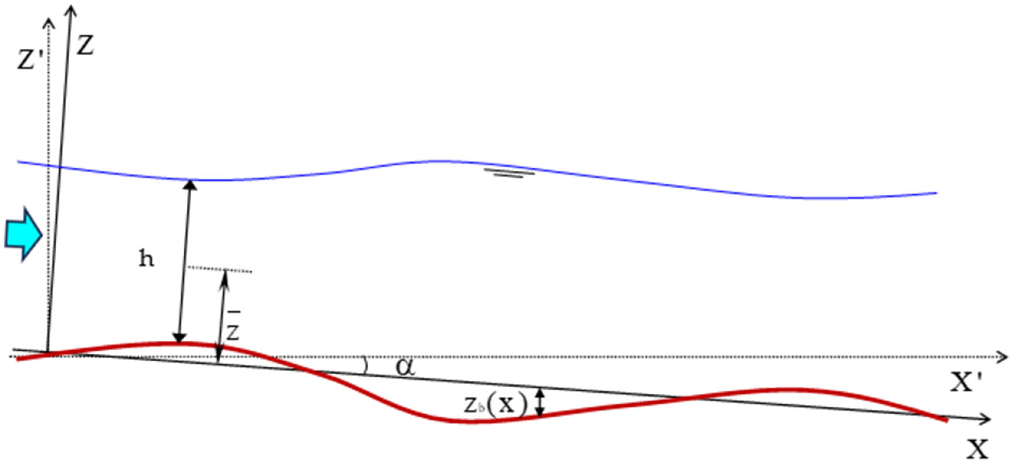
Based on the schematic illustration provided in Figure 1, the depth-averaged continuity and momentum equations under steady-state conditions are formulated within the inclined coordinate system defined by the axes X and Z. By invoking the small perturbation hypothesis, these governing equations can be linearized. Accordingly, the first-order approximations of the depth-averaged continuity and streamwise momentum equations are expressed as follows:
where x is the coordinate parallel to the averaged bed slope, ; is the local bed perturbation height measured from the averaged slope; h is the water depth; Uo is the depth-averaged velocity; F is the Froude number, ; and is the dimensionless Chezy coefficient. ; ; ; ; . The superscript (1) indicates the order of the parameter, (0) means the base or the mean value, whereas (1) refers to the perturbation.
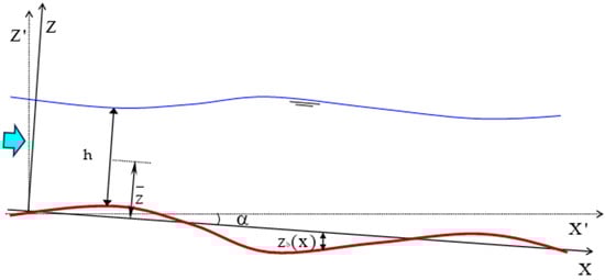
Figure 1.
Coordinate definition.
In this study, the bed load transport was estimated using Chang’s formulation, which is expressed as follows [40]:
In this context, denotes the volumetric bed load transport, while is an empirical coefficient reflecting sediment properties; a higher value implies that sediment particles are more readily for entrainment as bed load. For beds composed of medium to coarse sand, typically approaches 0.1. represents the specific weight of sediment, is the applied bed shear stress, and is the critical shear stress threshold for sediment motion. For analytical simplicity, is assumed to be negligible, a simplification more appropriate for fine sediments than for coarser grains. By combining Equation (3) with the (Exner-like) sediment continuity condition, Equation (4) is obtained, which reveals that an accelerating flow (i.e., >0) induces a reduction in bedform amplitude, thereby promoting bed perturbation damping.
Here, t is the time coordinate, is the normalized time = , n represents the sediment porosity, while denotes the ratio of water density to that of the sediment particles. From Equations (2) and (4), the momentum equation can be rewritten as:
Equation (5) constitutes an eigenvalue problem for determining the perturbation wave speed, C, under the assumption that the initially planar erodible bed undergoes a slight perturbation as described by Equation (6). Hereafter, will be denoted as h for simplicity.
The real and imaginary components of the bed wave speed can be determined as follows:
A positive imaginary component of the bed wave speed indicates that the perturbation will grow over time, whereas a negative value implies decay and stability of the initially planar bed. The normalized components of wave speed, given in Equations (7) and (8), depend on the Froude number (F), dimensionless wave number (kh), bed roughness parameter, and various sediment properties.
Equation (7) characterizes the migration behavior of bed perturbations; it demonstrates that bedforms propagate downstream when F < 1 and upstream when F > 1. Furthermore, Equation (8), which describes the normalized imaginary component of the wave speed, consistently yields negative values for all combinations of F and kh. This result implies that any imposed bed perturbation will diminish over time, ultimately restoring the bed to its original planar configuration. These findings suggest that the classical Saint-Venant equations do not predict the emergence of unstable bed modes under the considered conditions. This conclusion is in agreement with earlier studies conducted by several researchers [22,23,27].
3. Effect of SV Equation (SVE) Enhancements
3.1. Linearized Form of SVE with Non-Hydrostatic Terms (Case 1)
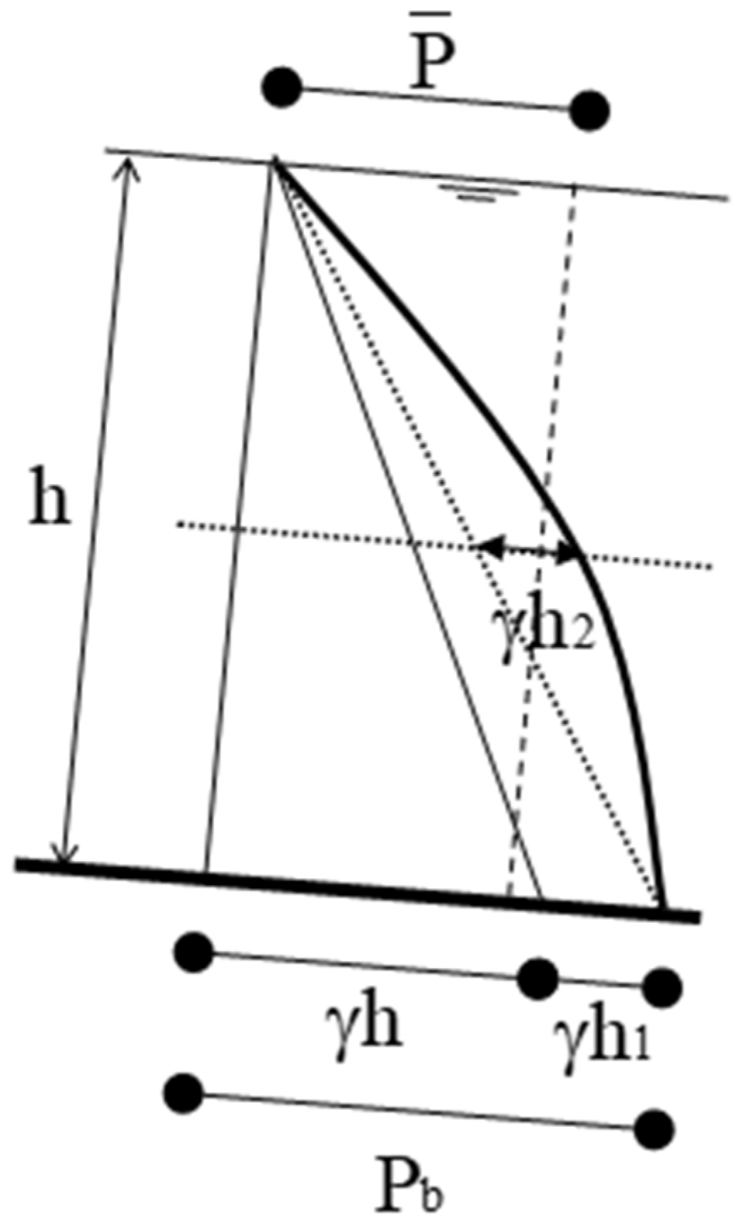
An important enhancement to the conventional Saint-Venant depth-averaged model involves accounting for non-hydrostatic effects in the pressure distribution. To incorporate these effects, a quadratic pressure distribution is assumed, as illustrated in Figure 2, a methodology previously adopted by a number of researchers, such as [32]. As a result, two additional degrees of freedom, denoted by h1 and h2, are introduced to the standard linear hydrostatic pressure profile.

Figure 2.
Pressure distribution including the non-hydrostatic effect.
To close the system of equations, two additional relations are required. Appropriate choices for these are the depth-averaged vertical momentum equation and the depth-averaged vertical moment of momentum equation. By assuming a uniform vertical profile for the downstream velocity, these equations can be considerably simplified and formulated as follows [32,34]:
Accordingly, the vertically averaged momentum equation in the streamwise (x) direction can be written as:
From Equations (6) and (10), the bed wave speed can be decomposed into its real and imaginary components, which are given as follows:
The discussion and comments on Equations (11) and (12) are given in Section 4.
3.2. Linear Stability Formulation of the VAM-Hydrostatic Model (Case 2)
In 1993, Ref. [32] introduced the vertically averaged and moment (VAM) model, a one-dimensional formulation that combines depth-averaged and moment-based components. The moment equations are obtained by vertically integrating the continuity and momentum equations, each multiplied by the vertical coordinate prior to integration.
In this subsection, a linear stability analysis is conducted for the VAM equations under the assumption of hydrostatic pressure conditions, hereafter referred to as the VAM-hydrostatic case. The effects of non-hydrostatic pressure will be examined in the following subsection (Case 3). In addition, this analysis adopts the recently developed moment-based Chezy formula for predicting bed shear stress, as proposed in [33]. The moment-based Chezy formula is expressed as:
where is a dimensionless coefficient defined as ; is another dimensionless coefficient that varies linearly with the roughness ratio h/zo; for more details about the significance of this coefficient, the reader is to refer to [33]; ; and is the Von Karman constant.
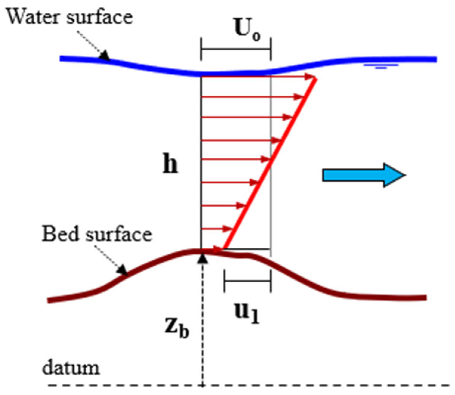
The term denotes the surface velocity in excess to the depth-averaged velocity, assuming a linear velocity distribution, as illustrated in Figure 3. Notably, when Kr = 0, Equation (13) simplifies to the conventional Chezy formulation for shear velocity. The moment-based Chezy approach has demonstrated improved predictive capability for spatial variability in bed shear stress, particularly over non-uniform bed topographies [33].

Figure 3.
Definition of u1.
The linearized form of the depth-averaged streamwise momentum equation, incorporating the shear stress representation given in Equation (13), yields Equation (14). Notably, when the calibration coefficient Kr is set to zero, Equation (14) simplifies to the classical form shown in Equation (2). The depth-averaged moment of momentum equation can further be expressed in a dimensionless form, as shown in Equation (15), where the eddy viscosity parameter Fe is defined by Fe=νt/(u∗·h), with νt representing the eddy viscosity. By combining Equations (1) and (13) and applying the sediment continuity relationship (Exner equation), Equation (16) is obtained. Collectively, Equations (1) and (14) through (16) can be consolidated into a coupled system of two equations with two unknowns. This system represents an eigenvalue problem used to solve for the complex wave speed C, as outlined in Equations (17) and (18).
If the calibration coefficient is set to zero, Equation (14) reduces to Equation (2).
The depth-averaged x-moment of momentum equation can be written in a dimensionless form as:
The coefficients through generally depend on the Froude number, the dimensionless coefficient (), the dimensionless Chezy coefficient, and sediment properties. Their explicit expressions are provided in Appendix A, while the complete derivation of Equations (17) and (18) is detailed in Appendix B.
3.3. Linear Stability Formulation of the Non-Hydrostatic VAM Model (Case 3)
As outlined earlier in Section 3.1, the influence of non-hydrostatic pressure components on the momentum equation is incorporated by assuming a quadratic pressure distribution, as illustrated in Figure 2. This assumption introduces two additional variables, h1 and h2, thereby necessitating two supplementary equations to close the system. These are provided by the depth-averaged vertical (z-direction) momentum equation and the depth-averaged vertical moment of momentum equation.
The depth-averaged z-momentum equation is given by Equation (19), where u′ = U(z) − Uo; w′ = W(z) − Wo; τ denotes shear stress; and the overbar indicates a depth-averaged quantity. Among the terms on the right-hand side of Equation (19), the first is the most dominant. The second term becomes more relevant in the case of fully developed bedforms but, due to its minimal effect in the context of small-amplitude perturbations, it is disregarded in the present linear analysis. Equation (19) establishes a relationship between the dynamic pressure term h1 and the spatial gradient of the depth-averaged vertical velocity Wo, which can be determined using the continuity moment equation, represented by Equation (20).
Here, z′ = z − , where . denotes the centroid of the flow depth measured from the perturbed bed. Assuming a linear vertical profile for the streamwise velocity component, the vertical momentum equation (Equation (19)) can be simplified accordingly to Equation (21).
The vertically averaged moment of momentum equation in the vertical (z) direction can be formulated as:
By omitting the shear stress contributions along with other nonlinear and non-dominant terms, Equation (22) can be simplified, through the application of Equation (20), to yield Equation (23). This equation features the term , which can be approximated by assuming a parabolic distribution for the vertical velocity component (refer to Appendix A for more details). Following further algebraic simplifications, Equation (23) leads to the reduced form presented in Equation (24).
Accordingly, the linearized streamwise momentum equation, now accounting for non-hydrostatic pressure effects, takes the form of Equation (25). This equation can be further simplified, resulting in Equation (26).
Additionally, the depth-averaged x-moment of momentum equation may be expressed in dimensionless form, as follows:
It is noteworthy that the influence of the h2 term appears explicitly in the x-momentum equation (Equation (25)) but is absent from the x-moment of momentum equation (Equation (27)). This is attributed to the fact that h2 represents the parabolic portion of the pressure distribution, which is symmetric about the flow’s mid-depth, as illustrated in Figure 2, and produces no net moment within the linearized framework.
By combining Equations (1), (16), (19), (26), and (27), the governing system can be reduced to a pair of coupled equations involving two unknowns. This formulation constitutes an eigenvalue problem for the perturbation wave speed C, with the complete mathematical expressions detailed in Appendix A.
4. Results and Discussion
The analysis results are conveyed through the predicted directions of bedform migration during evolution and, more critically, the growth or decay rate of bedform amplitude. This rate is illustrated using stability diagrams, which display contour lines of the normalized growth rate (Cim/Uo) within the kh–F parameter space. Each diagram corresponds to specific values of the roughness parameter (), the dimensionless coefficient (C∗), and sediment characteristics.
4.1. Migration Direction of Evolving Bedforms
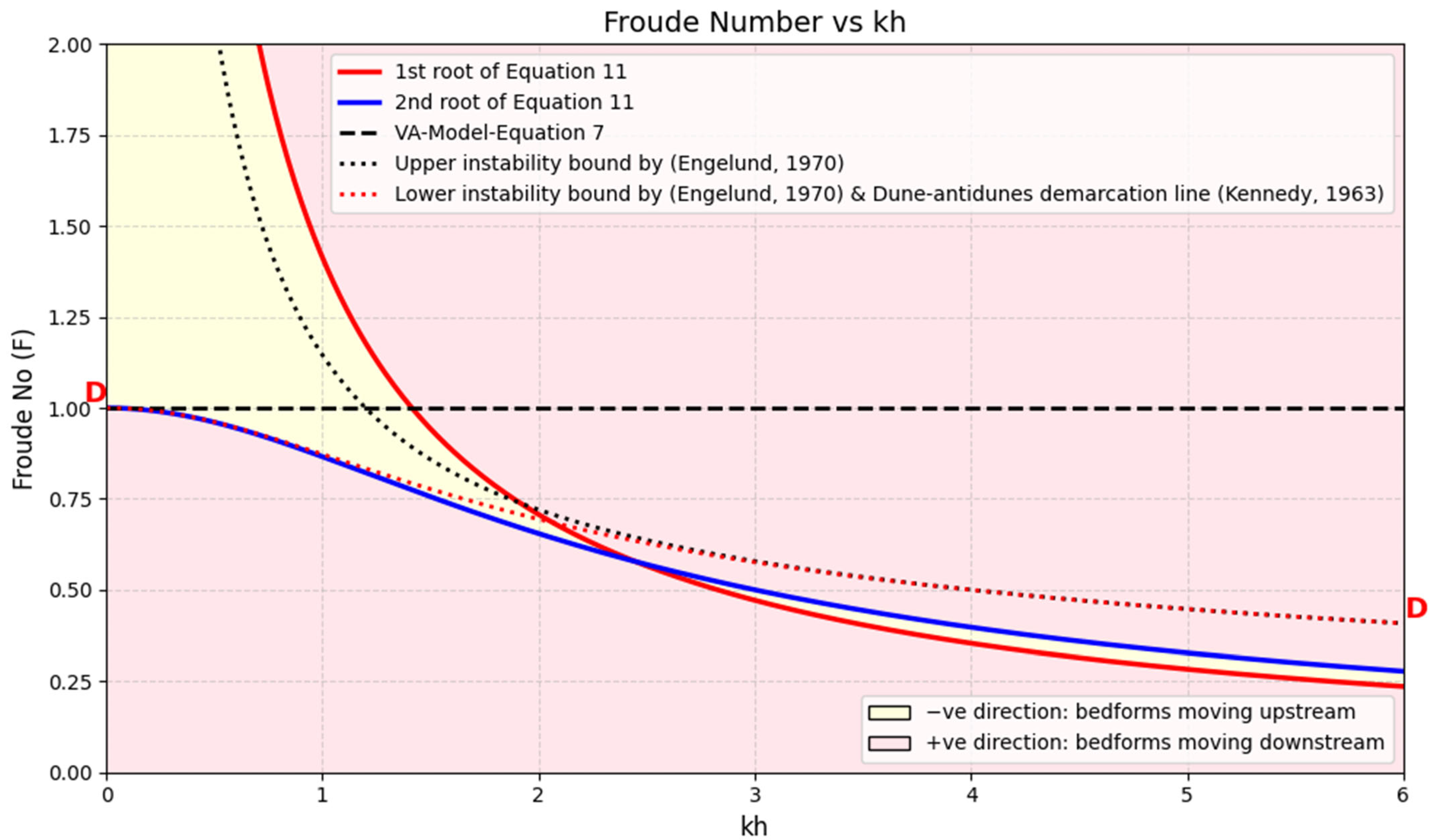
Figure 4 illustrates the predicted bedform migration directions during their evolution, comparing outcomes derived from the conventional depth-averaged Saint-Venant (SV) model (Equation (7)) with those from the modified formulation that incorporates non-hydrostatic pressure terms (Equation (11)). The figure plots the bed wave propagation direction as a function of the dimensionless wave number and Froude number kh and F, respectively. Additionally, the results are benchmarked against Kennedy’s established criterion delineating the maximum Froude number threshold for dune formation (that are known to propagate downstream), represented by the dotted line labeled D-D [9].
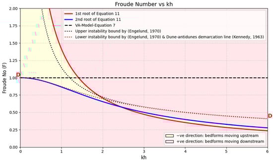
Figure 4.
Estimated direction of bed wave perturbation. (for conventional SVE and SVE with non-hydrostatic terms).
The curves presented in the figure clearly indicate the transitions between downstream-moving and upstream-moving bedforms. These demarcation lines were calculated from their corresponding expressions for Creal/Uo (Equation (7) for the dashed line and Equation (11) for the solid lines) by enforcing the condition Creal/Uo = 0.
The importance of incorporating non-hydrostatic pressure effects becomes evident from the comparative analysis presented in Figure 4. These effects result in more physically realistic predictions of bed wave direction across the full range of wavenumbers considered. The revised model significantly improves predictive performance over the conventional hydrostatic Saint-Venant–Exner (SVE) model (Equation (7)), underscoring the critical role of non-hydrostatic terms in accurately representing bedform dynamics.
Figure 4 illustrates the demarcation line between dune and antidune regimes predicted by the conventional hydrostatic SVE model, shown as a horizontal dashed black line at F = 1. This line deviates notably from the empirically established boundaries proposed by Kennedy and Engelund, depicted as dotted brown and black lines, respectively. When non-hydrostatic effects are included, based on Equation (11), the resulting demarcation lines (shown in red and blue) more closely align with those of Kennedy and Engelund, demonstrating the improved physical realism of the non-hydrostatic depth-averaged formulation.
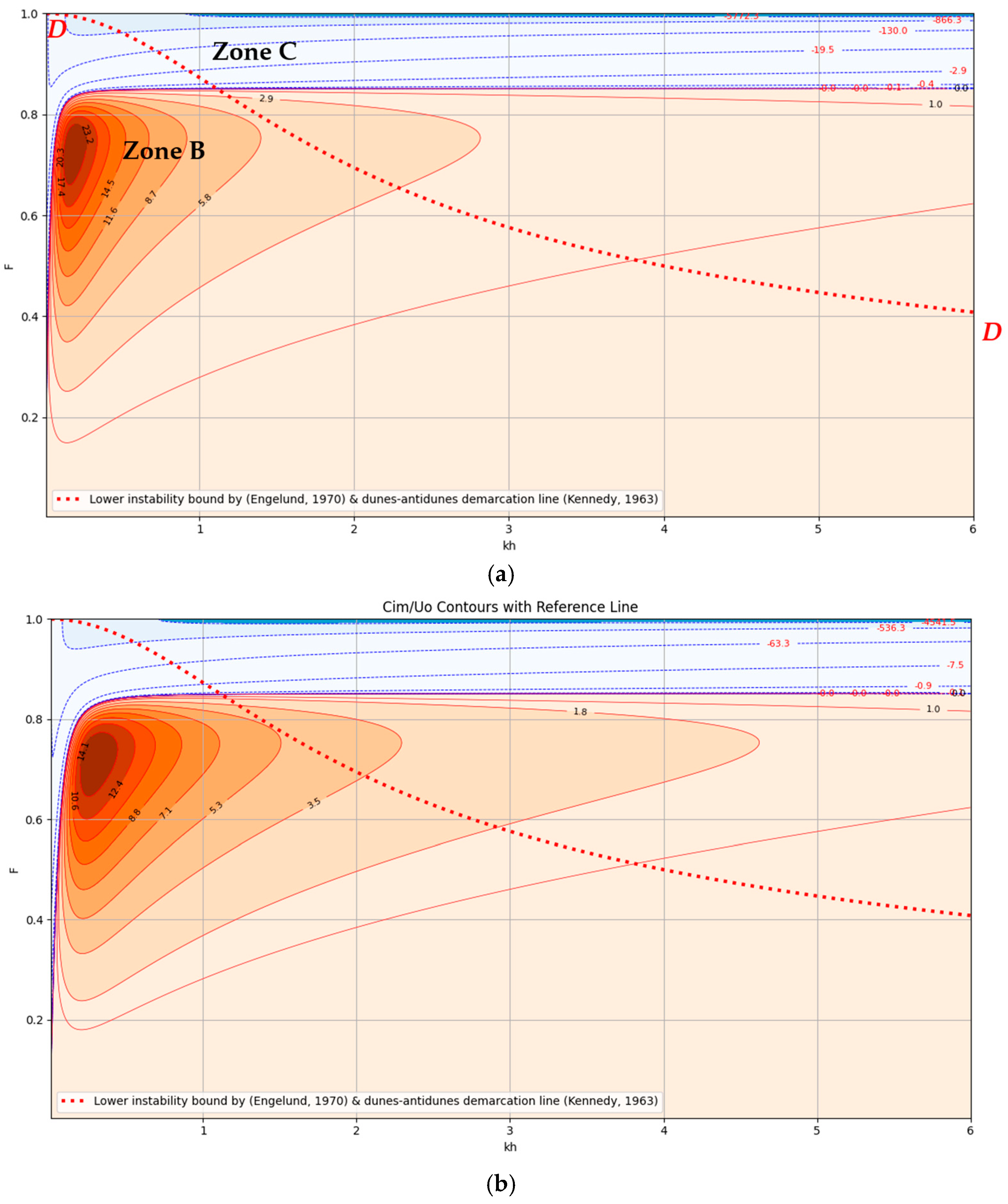
Figure 5 presents the normalized contour map of the real component of the perturbation wave speed, Creal/Uo, plotted within the kh–F parameter space using the VAM equations that account for non-hydrostatic effects. The results correspond to the case where = 2.0, = 15, and = 0.07. The figure specifically highlights the behavior in the low-Froude-number regime (F < 1). Additionally, the diagram includes Kennedy’s demarcation boundary (denoted as line D–D), which distinguishes between downstream-migrating dunes and upstream-migrating sand waves.
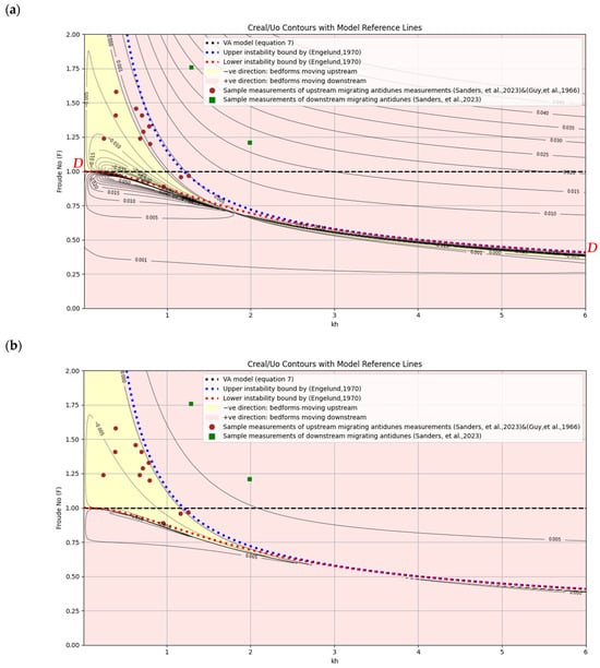
Figure 5.
Normalized bed wave speed contour lines (Creal/Uo) for VAM equations considering the non-hydrostatic effects. (a) ( = 2.0, = 15, = 0.07), (b) ( = 1.3, = 17, = 0.15).
Figure 5a presents contour plots of the normalized real part of the wave perturbation velocity, Creal/Uo, across the kh–Froude number parameter space. These results are derived from the VAM equations that include non-hydrostatic pressure effects, using the parameter set, = 2.0, = 15, and = 0.07. While the scope of the current analysis is confined to low-flow subcritical conditions, part of the supercritical regime is also depicted to facilitate direct comparison with Figure 4. The figure includes Kennedy’s empirical demarcation line (labeled D–D), which delineates downstream-migrating dunes from upstream-migrating sand waves, along with Engelund’s lower and upper instability limits (shown as red and blue dotted lines). The close agreement between the model-predicted transition boundaries and those proposed by Kennedy and Engelund highlights a substantial improvement over predictions from the Saint-Venant equations, even when enhanced with non-hydrostatic terms.
Although this study primarily focuses on bedforms within the low-flow regime, it is worthwhile to preliminarily evaluate the VAM model’s predictive performance under high-flow conditions, particularly in capturing antidune migration direction. To this end, recent experimental data from [41] were employed for model validation. Table 1 summarizes the experimental runs where antidunes were observed to migrate either upstream or downstream.

Table 1.
Characteristics of sample measurements of antidunes traveling in both directions [41].
The initial validation utilized the modern dataset of Sanders et al., which was generated using high-resolution techniques such as laser scanning, sonar, and acoustic Doppler profiling—offering enhanced spatial and temporal accuracy. By contrast, the classical dataset compiled by [42] relied on point gauge measurements, often taken after draining turbid flows, which may introduce notable uncertainties. Nevertheless, we acknowledge the foundational role of Guy’s work and have incorporated all upstream-migrating antidune cases from his dataset into our analysis, along with their corresponding hydraulic parameters. These cases have now been added to the revised Figure 5a.
While some deviation between the model predictions and the experimental antidune data is observed under the default parameters ( = 2.0, = 15, and = 0.07), improved alignment is achieved in Figure 5b after adjusting the model parameters to ( = 1.3, = 17, and = 0.15). This observed sensitivity to parameter values underscores the importance of careful calibration, an issue that warrants focused attention in future investigations.
Remarkably, the VAM model accurately predicted the direction of antidune migration in both upstream- and downstream-moving cases.
Figure 5 illustrates that the dimensionless phase speed Creal/Uo increases with increasing wavenumber kh, implying that shorter wavelength bedforms (i.e., those with smaller values of λ) migrate more rapidly than their longer-wavelength counterparts. This observation aligns with established findings in fluvial geomorphology, where smaller bedforms are generally observed to travel at higher rates compared to larger ones [43,44,45,46,47].
Supplementary Figures S1 and S2 present additional contour plots of Creal/Uo across a range of Chezy roughness coefficients (). The results show that increasing expands the region in which antidunes migrate upstream. This behavior is consistent with hydraulic theory, as higher values correspond to reduced bed resistance, which weakens flow–bedform interactions and lowers the energy required for upstream migration.
4.2. Bedform Evolution Analysis Based on the Hydrostatic VAM Model
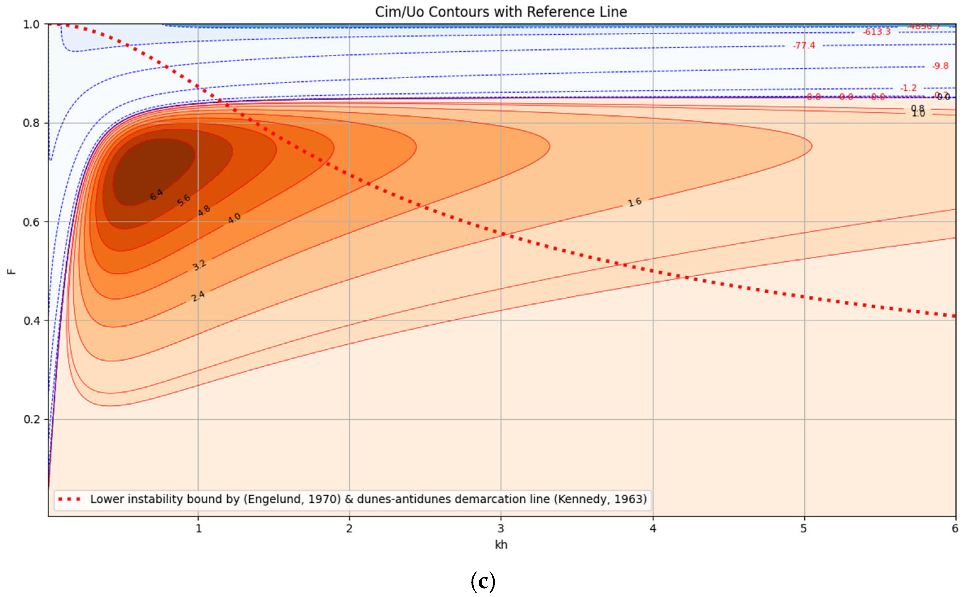
Figure 6 and Supplementary Figures S3–S5 present stability diagrams (SDs) from the VAM-hydrostatic linear stability analysis (Equation (18)). These SDs show contours of normalized growth rate, Cim/Uo, across kh–Froude number space, with each diagram corresponding to parameter sets (, , , and sediment properties). All SDs consistently reveal two distinct regions separated by a near-horizontal boundary: an upper decay zone (Zone C, negative growth) and a lower growth zone (Zone B, positive growth signaling bedform development).


Figure 6.
Stability diagram (contour lines of 105 × Cim/Uo) for VAM-hydrostatic equations, = 2.5, = 15, (a) = 0.07, (b) = 0.15, and (c) = 0.4.
Critically, while the non-hydrostatic Saint-Venant equations (SVE) model (Equation (12)) predicts no positive growth, confirming its inability to simulate bedform initiation, the VAM-hydrostatic model identifies growth within low-Froude regimes (Zone B). This demonstrates the superior physical fidelity of VAM’s shear stress formulation (Equation (13)), which captures the phase lag between bed shear stress and topography evolution. By resolving this key mechanism, VAM enables depth-averaged frameworks to simulate bedform onset, advancing their utility in sediment transport and morphodynamic modeling.
Although the boundary between Zones B and C appears overly simplified compared to the curved demarcation lines given by Kennedy and Engelund (red dotted lines in Figure 6), the ability to predict positive growth marks a significant advancement for depth-averaged models in sediment transport and morphodynamics. Nonetheless, further refinement is needed, particularly for dynamic simulations involving full sediment–flow interactions, as discussed in the following subsection.
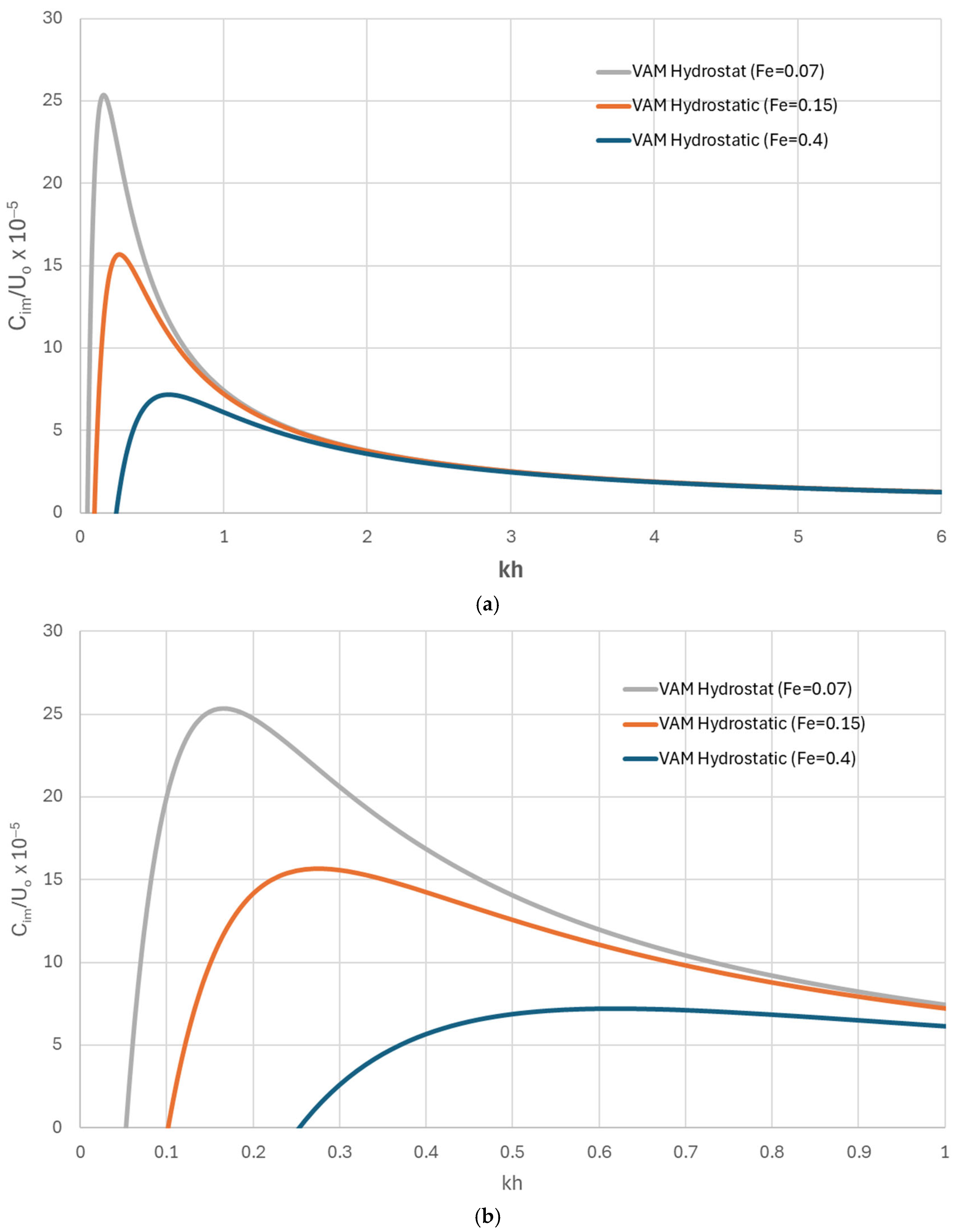
Within the region exhibiting positive growth rates, a distinct wavenumber emerges as the dominant mode responsible for the amplification of bedform disturbances. This most unstable wavelength is associated with Zone B of the stability diagrams. Figure 7a,b illustrate horizontal transects of the stability contours presented in Figure 6, extracted at a fixed Froude number of F = 0.7. The results indicate that the VAM-hydrostatic model predicts a single, well-defined instability mode corresponding to dune-type bedforms.
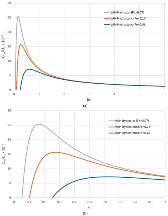
Figure 7.
Horizontal transects of SD (shown in Figure 6) taken at F = 0.7. (a) kh ranges from 0 to 6. (b) kh ranges from 0 to 1.
Figure 7b provides a magnified view of Figure 7a, offering clearer insights into the influence of the turbulent eddy viscosity parameter (). As increases from 0.07 to 0.4, a systematic reduction in the maximum growth rate is observed—consistent with theoretical expectations. Concurrently, the corresponding dominant wavenumber increases from approximately kh ≈ 0.16 to kh ≈ 0.61, indicating a shift toward shorter bedform wavelengths with increasing turbulence intensity. The effect of could be justified as the turbulent eddy viscosity coefficient controlling the intensity of momentum diffusion by turbulence. A higher eddy viscosity means stronger turbulent mixing of momentum, which smooths out velocity gradients and diminishes flow separation and inertia effects over bed undulations. Physically, turbulent diffusion transfers momentum more efficiently from faster to slower flow regions, so the flow becomes less perturbed by small-scale bed variations, which has a direct damping effect on the growth of bedforms. The influence of on the dominant wavenumber is consistent with previous studies, which have emphasized the role of turbulence characteristics in determining the emergent wavelength of flow instabilities [43].
4.3. Bedform Evolution Analysis Based on Non-Hydrostatic VAM Formulation
The linear stability analysis results of the fully dynamic non-hydrostatic VAM formulation are presented through a series of stability diagrams (SDs) generated for various combinations of the roughness parameter (), the momentum correction coefficient (), and the eddy viscosity factor (). Representative examples are shown in Figure 8a–c, while a broader set appears in the Supplementary Materials (Figures S6–S20). These diagrams are based on the imaginary component of the wave speed for the bed perturbation given in Equation (A45). To facilitate reproducibility, a Python 3 script was developed to generate SD plots for any user-defined combination of the governing parameters.

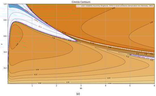
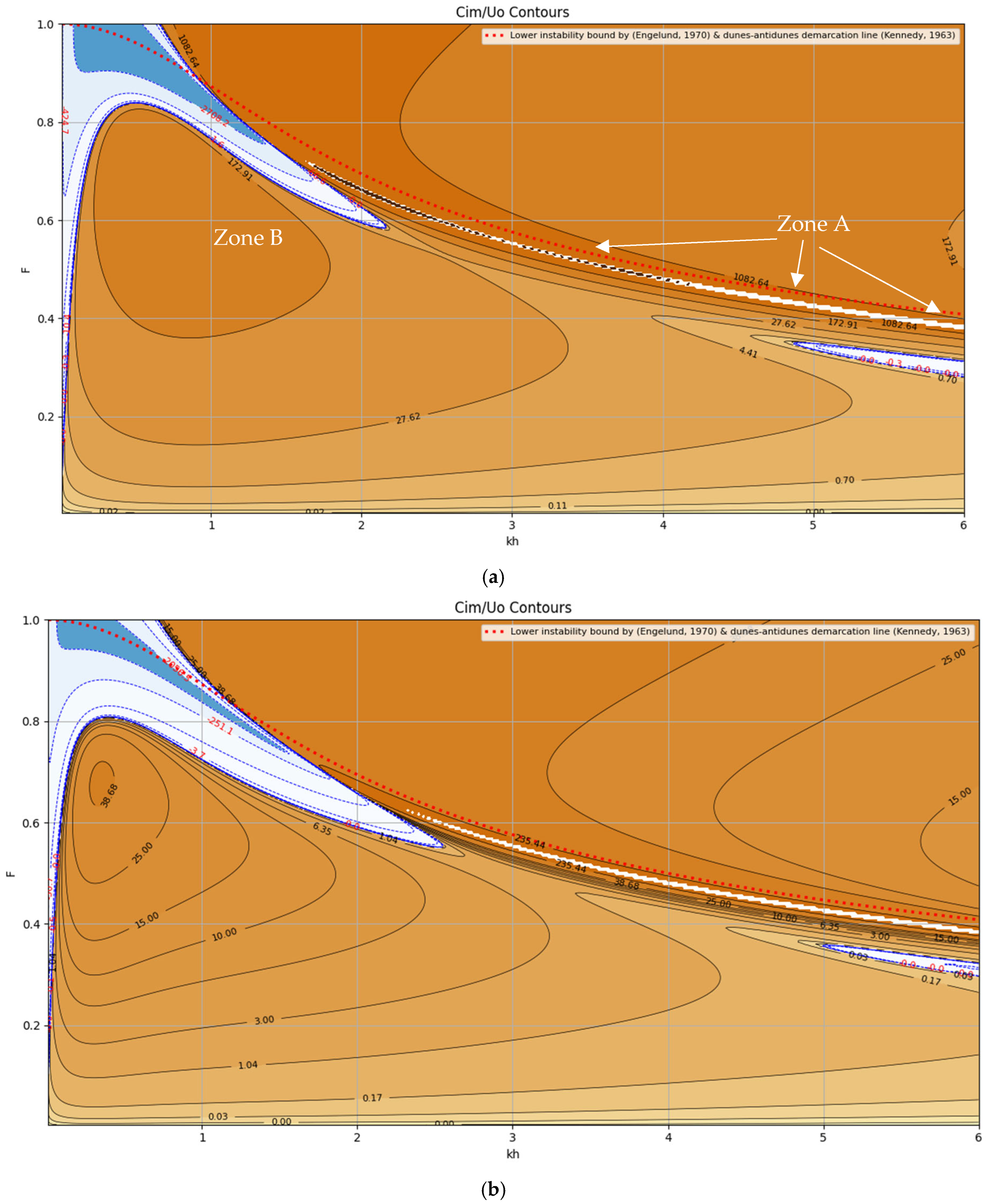
Figure 8.
Stability diagram (contour lines of 105 × Cim/Uo) for VAM equations, = 2.0, = 0.2. (a) = 10, (b) = 15, and (c) = 20.
Figure 8a–c display normalized growth rate contours (Cim/Uo) for the case = 2.0 and = 0.2 under three roughness scenarios ( = 10, 15, and 20). Regions with positive growth rates are indicated by brown-gradient contours, while areas of decay are shaded in blue. Two distinct instability zones are consistently observed below the Kennedy and Engelund demarcation curves (shown as dotted red and blue lines):
Zone A–A emerges just below the instability threshold identified by Kennedy and Engelund and is not predicted by the hydrostatic formulation (presented in Section 4.2). It corresponds to high wavenumbers (i.e., shorter wavelengths), which are indicative of ripple-like features.
Zone B represents the dune instability regime observed in previous hydrostatic cases and is associated with lower wavenumbers, corresponding to longer bedform wavelengths.
These zones identify preferential wavelengths where bedform disturbances are most likely to grow under low-Froude conditions. In contrast, the upper-left region of the diagrams consistently exhibits Zone C, a decay zone indicative of morphodynamic stability typically associated with plane bed configurations or washed-out dunes.
An important visible trend across Figure 8a–c is the inverse relationship between and growth magnitude. As roughness decreases (i.e., higher ), interaction between the flow and the bed weakens, leading to a reduced tendency for bedforms to grow. This behavior emphasizes the role of bed resistance in modulating instability dynamics.
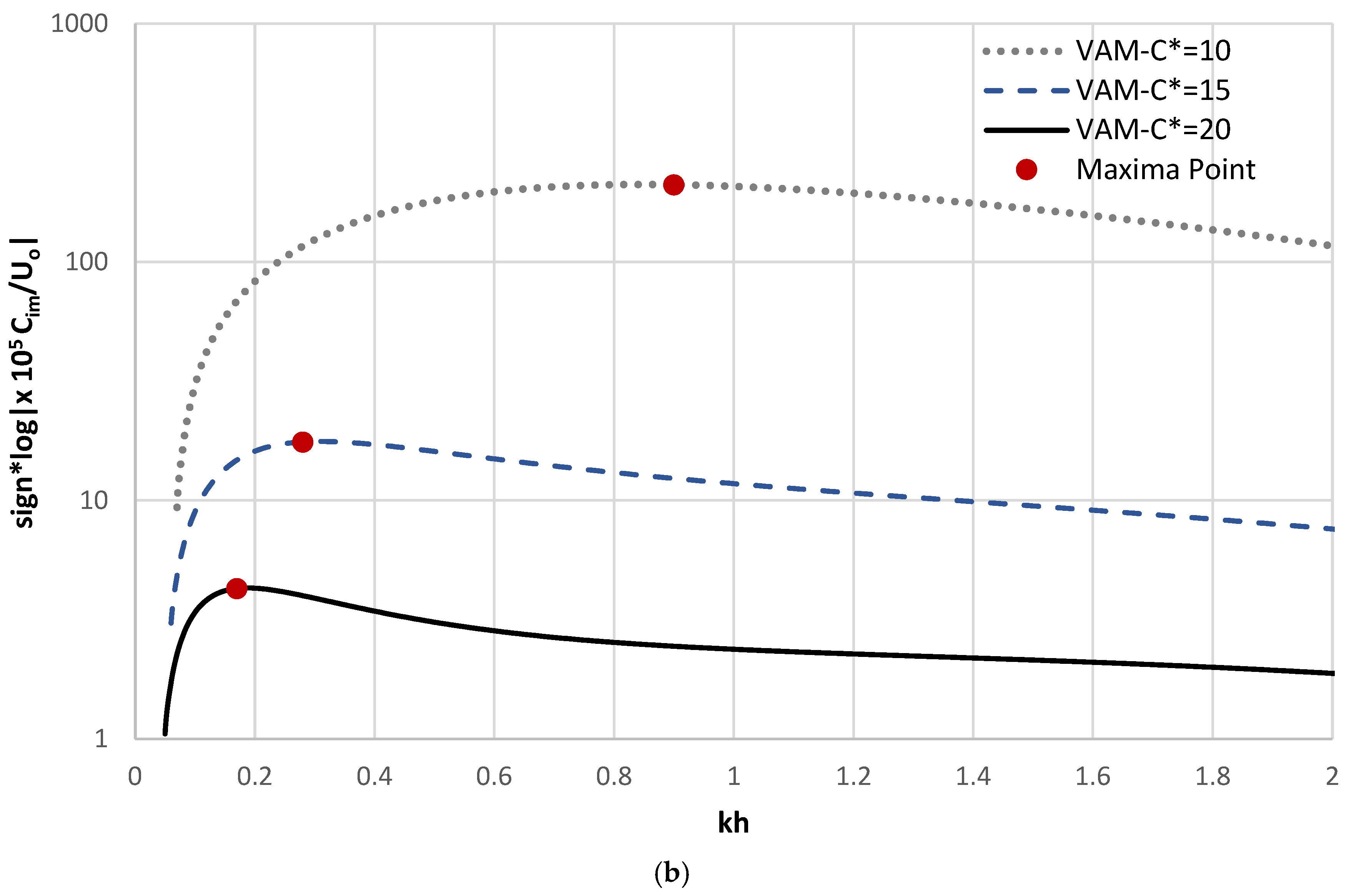
Figure 9a,b provide horizontal cross-sections of the growth rate contours at a fixed Froude number (F = 0.4) for the three values. The plots use a logarithmic vertical scale to highlight the variations in growth rate across wavenumbers. The results confirm the presence of dual instability peaks, one associated with ripples (Zone A–A) and another with dunes (Zone B). As decreases (from 20 to 10), both the growth rate and dominant wavenumber increase, with peak values shifting from kh ≈ 0.17 to 0.9. These findings suggest that rougher beds promote the formation of shorter, faster-growing bedforms, while smoother beds promote longer, slower-growing dunes or stable flat beds, an observation that is consistent with previous experimental and theoretical studies [13,18,19].
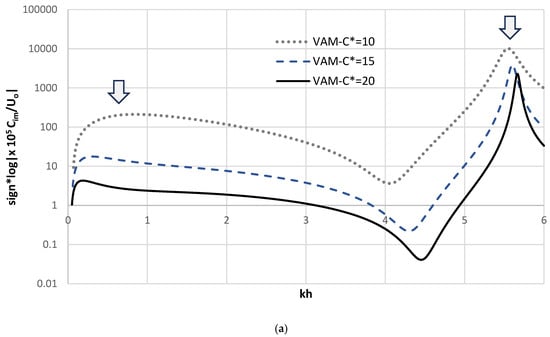
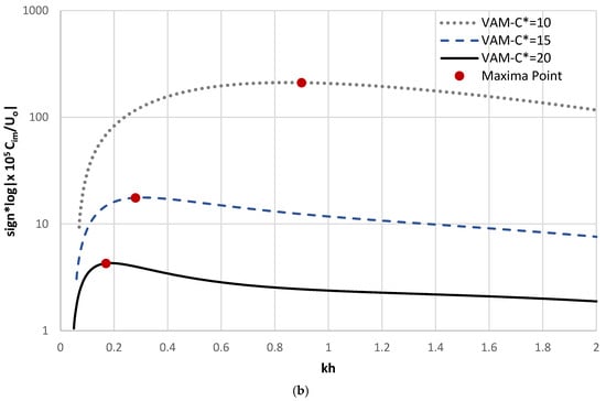
Figure 9.
Horizontal transects taken at Froude No F = 0.4 for three VAM stability diagrams drawn for = 2.0, = 0.2 and different bed roughness : (a) kh = 0 to 6, (b) kh = 0 to 2 (zoom in). (note: the arrows in (a) point to the locations of the dual peak values).
Furthermore, the critical (i.e., maximum) Froude number at which dune (of wavelength 6 times the water depth) growth ceases decreases with increasing , approximately at a maximum F = 0.75 for coarse sand ( = 10), F = 0.725 for medium sand ( = 15), and F = 0.70 for fine sand ( = 20), as seen in Figure 8a–c. A similar trend was previously reported by Fredsøe [19] in his linear stability work.
It is also worth noting that the growth rate associated with Zone A is typically larger than that of Zone B. Given its association with shorter wavelengths, Zone A may represent the initial seed formations of ripples or sand wavelets that evolve into dunes.
As shown in Supplementary Figures S3–S5, the coefficient plays a critical role in controlling instability characteristics. Reducing lowers the maximum growth rate and shifts the instability boundary downward, effectively reducing the unstable region. At = 0, the governing Equation (18) simplifies to Equation (8), and no bed instabilities are observed. For further discussion on the factors affecting , readers are referred to references [33,37].
Although the VAM-hydrostatic model succeeds in identifying growth zones, it predicts an unrealistic horizontal boundary between stable and unstable regimes, deviating from the more physically consistent demarcations proposed by Kennedy and Engelund. In contrast, the inclusion of non-hydrostatic effects in the VAM framework aligns the model’s predictions more closely with empirical evidence, providing a more accurate and physically grounded representation of bedform evolution.
It is also important to note that the wavelength of bed perturbations associated with instability Zone B exhibits a clear dependence on flow depth. In contrast, the wavelength characteristics of ripples, corresponding to Zone A–A, appear to be largely independent of water depth. Investigating the extent to which the ripple-scale bedform wavelengths in Zone A–A may still exhibit subtle sensitivity to flow depth remains an interesting direction for future research.
Zone A-A could be approximated by:
This relation could be reduced as follows to give an estimate for the wavelength of the ripples ():
Finally,
The parameters and s represent the dimensionless critical shear stress and the specific gravity of sediment particles, respectively. As expressed in Equation (30), the wavelength λr associated with bed perturbations in Zone A–A appears to be largely independent of flow depth and is primarily governed by bed roughness, which, in turn, is a function of the sediment grain size. For a range of 1 < / < 10 and a Chezy resistance coefficient = 15, Equation (30) predicts values on the order of (100 to 1000) times . These predictions are consistent with empirical observations of sand wavelets, where ≈ 175 (with in millimeters) as reported in [44], and sand ripples, where ≈ 1000, as noted in [45].
4.4. Comparison with Bedform Measurements
4.4.1. Dominant Wavelengths for Ripples
To evaluate the accuracy of the LSA based on VAM model, experimental datasets for ripples from previous studies such as [46,47,48] were utilized. These experiments involved measurements of ripple geometry developed in fine sand beds.
Figure 10 shows the variations in the normalized dominant ripple wavelength with the Shields parameter . The figure compares the measurements with the results of Equation (30) that was approximately deducted from VAM LSA. Also, the proposed model previously developed by Boes and Dey [29] is added for comparison. The comparison shows that Equation (29) can reasonably predict the dominant wave lengths of the evolving ripples; however, the predictions are significantly affected by the value of .
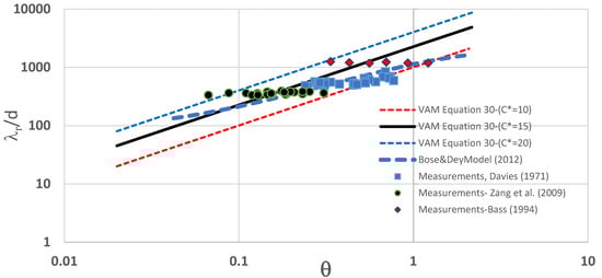
Figure 10.
Variation in the normalized dominant ripple wavelength with the Shields parameter. (note, data comparison from: Boes and Dey [29], Davies [46], Bass [47], Zang et al. [48]).
4.4.2. Dominant Wavelength for Dunes and Low-Flow Regime Sand Waves
To facilitate a comparative evaluation of the LSA-VAM model predictions with observed low-flow regime sand waves and dunes, 10 experimental datasets were compiled from the literature. The key characteristics of these datasets are summarized in Table 2.
Table 2.
Laboratory experiments for low-flow bedforms.
Figure 11 presents the stability diagram for the LSA-VAM model in the case of = 10, = 1.0, and = 0.2. The diagram also shows the experimental data of all the laboratory experiments recently reported in the last two decades as per the characteristics given in Table 2. It is interesting to note that most of the data points lie in the positive-growth-rate area and outside the negative-growth-rate zones. It is also of interest to notice that the data seems to be arranged on and around the polyline tracing the ridges of the local positive growth rate (shown in dashed yellow color), which could be an indicator of the LSA-VAM model despite its simplifications, but it generally captured correctly the modes of instabilities for the low-flow regime case quite well.
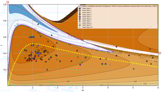
Figure 11.
Stability diagram based on the non-hydrostatic VAM equations with parameters = 10, = 1.0, and = 0.2. (presented contour lines of 105 × Cim/Uo) (note: the reference number for each data type shown in the legend corresponds to the same experimental number listed in Table 2) (dashed yellow line represents the maximum growth ridge line).
The results also highlight a noticeable sensitivity to the eddy viscosity parameter . Under uniform flow conditions over a flat bed, typically ranges between 0.06 and 0.08. However, in the presence of bedforms, particularly where flow separation is likely, this parameter tends to increase. For instance, spatial measurements from the fixed dune experiment T5 [59] revealed values of varying between approximately 0.17 and 0.22. It was observed that higher values of are associated with a reduction in the bedform growth rate and an increase in the dominant wavelength characterizing instability in Zone B.
4.5. Comparison with Colombini’s Analysis
The linear stability analysis conducted in this study using the non-hydrostatic, depth-averaged VAM equations offers a distinct modeling perspective compared to the work of Colombini [20], who extended the classical theories of Engelund and Fredsøe [60] using a two-dimensional vertical Reynolds-averaged framework. Colombini’s model evaluated bed shear stress at the top of the bedload layer, introducing an additional term associated with the longitudinal pressure gradient. This modification notably affects the imaginary component of the critical bed shear stress for determining instability, while having little influence on the real component. His formulation is grounded in Bagnold’s sediment transport theory and emphasizes the delicate balance between stabilizing and destabilizing forces governing dune and antidune formation.
While both studies aim to predict the emergence and growth of bedforms under varying flow conditions, their modeling assumptions and target phenomena differ significantly. Colombini’s analysis focused on dune and antidune regimes and did not address ripple-scale features. Consequently, his wavenumber range was limited to kh ≲ 1.5, whereas the present VAM-based framework explores instabilities up to kh ≈ 6 to capture ripple dynamics in the low-Froude regime. Notably, our analysis revealed the existence of dual instability modes, one associated with ripples (shorter wavelengths) and another with dunes (longer wavelengths), a feature not detected or discussed in Colombini’s work.
Moreover, Colombini included a correction for gravitational effects in the bedload transport formula, which was not incorporated in the present model. His results also pointed out that suspended load and sediment inertia are not essential for antidune formation, which has been proved in our study too, although they may alter the growth rate surface. Importantly, Colombini identified that, under quasi-steady flow assumptions, resonance-like artifacts could appear in the growth-rate diagrams. By introducing time-dependent terms into the flow equations, these unrealistic resonances were shown to disappear, while the overall shape and location of the instability zones remained only moderately affected.
Another key distinction is the presentation of results. Colombini’s stability diagrams do not include numerical growth rate contours, which limits direct quantitative comparison. Nonetheless, when adjusted for scale differences, the demarcation lines in Colombini’s results are broadly consistent with those obtained in the present study, especially in identifying the boundary between dune and antidune regimes.
5. Conclusions
This study presented a novel linear stability analysis (LSA) framework for simulating bedform evolution under low-flow conditions using a vertically averaged and moment (VAM) approach. By comparing four modeling configurations—ranging from the classical Saint-Venant shallow-water equations to the fully extended VAM model—this research highlights how incorporating additional physics markedly improves predictive performance. In particular, the extended VAM model includes non-hydrostatic pressure effects and a moment-of-momentum-based velocity profile representation, which together enhance the depth-averaged formulation. The theoretical analysis and numerical results consistently show that these extensions lead to a more robust prediction of the initial bedform growth and dynamics.
The comparative findings demonstrate that the standard hydrostatic Saint-Venant model (with depth-uniform velocity assumptions) has limited capability in capturing the onset of bedforms under low-flow, bedload-dominated conditions. In contrast, the fully extended VAM model successfully predicts the emergence of both small-scale ripples and larger dune-like features while using only bedload sediment transport. This is a significant outcome, as it shows that, even without invoking suspended-load mechanisms, the VAM-based framework can reproduce the formation of ripples and dunes. The improved performance of the VAM approach underscores the value of including vertical flow structure and pressure dispersion in the analysis, features that prove essential for generating the instabilities associated with natural bedform development.
A key insight from the VAM formulation is the natural introduction of a phase-lag mechanism between the flow field and the bed evolution. Unlike simpler depth-averaged models that often assume an instantaneous adjustment of sediment transport to changes in flow, the VAM-based model inherently produces a delayed response. This physically relevant phase lag means that the peak bed shear stress and sediment transport do not occur exactly in phase with the bed elevation perturbations. Such a delay is crucial for realistic bedform behavior; it stabilizes the growth of finite-wavelength features and prevents the unbounded amplification of very short waves. In essence, the present model captures the timing offset between flow forcing and sediment movement that is known to govern ripple and dune formation, doing so as an emergent property of the governing equations rather than through ad hoc empirical tuning.
This study also illuminates how key model parameters influence bedform growth rates and migration patterns. The Chezy friction coefficient (), the roughness parameter (), and the eddy viscosity factor () each play distinct roles in modulating the instability characteristics. A higher friction (lower or larger roughness) tends to dampen the growth of bedforms and can reduce their migration speed, as increased flow resistance curtails the intensity of sediment transport over evolving topography. Conversely, smoother flow conditions (higher or lower roughness) promote more vigorous instability growth, leading to faster-developing and more rapidly migrating bedforms. The eddy viscosity factor, which represents the degree of turbulent momentum diffusion, affects the relative amplification of different wavelength perturbations; larger eddy viscosity values suppress short-wavelength variations (acting as a stabilizing influence on small ripples) and shift the dominance toward longer waves, while lower eddy viscosity allows finer-scale features to grow more readily.
Importantly, the VAM-based model’s predictions show strong agreement with experimental observations for both ripples and dunes. The linear growth rates and most unstable wavelengths obtained from the analysis correspond closely with those observed in laboratory flume tests of ripple formation under low-flow conditions. Similarly, the model correctly predicts the trend toward longer wavelengths and slower growth rates, in line with measured dune datasets. The migration directions and relative celerities of the bedforms are also captured correctly (with downstream migration for these subcritical flow bedforms), matching qualitative observations. This level of agreement indicates that the model not only reproduces the expected behavior of bedform instability theory but also aligns quantitatively with real-world data, lending credence to its underlying assumptions and computational implementation.
The developed VAM-based LSA framework significantly advances the capabilities of depth-averaged morphodynamic modeling. By naturally integrating non-hydrostatic pressure distribution effects and a depth-varying velocity profile into a traditionally depth-averaged approach, the model bridges a critical gap between simple shallow-water equations and more complex three-dimensional simulations. The outcome is a more physically faithful yet computationally efficient tool for predicting initial bedform evolution under sediment transport by bedload.
6. Limitations and Outlook
This study has demonstrated the enhanced capability of the non-hydrostatic VAM framework over the conventional Saint-Venant (SV) depth-averaged model in analyzing bedform instabilities, particularly within low-flow regimes. Nevertheless, several limitations must be acknowledged when interpreting and applying these findings.
The current analysis focuses exclusively on bedforms occurring under low-Froude-number conditions (F2 ≪ 1), specifically ripples and dunes. As such, the conclusions drawn cannot be directly extended to high-flow regimes, such as those involving antidunes or other complex morphodynamical features. Future research should address the dynamics of bedforms under high-Froude conditions to broaden the scope of the model’s applicability.
The model assumes a one-dimensional representation of bedforms with a constant channel width. Expanding the approach to two-dimensional bedforms, which introduces additional geometric and hydrodynamic complexities, would provide a more realistic framework for practical applications and warrants further investigation.
Only bed load transport was considered in this analysis. The exclusion of suspended sediment transport limits the comprehensiveness of the predictions, particularly in flows where suspension dominates the sediment transport regime. Future work should integrate both transport modes for a more holistic sediment dynamics model.
The current formulation assumes quasi-steady flow conditions based on the rationale that the flow adjusts much more rapidly than the bed morphology evolves. While this assumption is valid in many fluvial applications, it may be overly restrictive in dynamic environments such as estuaries, tidal inlets, dam-break scenarios, or situations involving rapidly evolving free-surface waves. In such cases, the coupling between flow and bedform development may require the use of fully unsteady flow equations. Future studies should consider applying the unsteady VAM framework to assess model performance under these more complex conditions.
The analysis relies on linear stability theory, which, while effective in capturing the initial emergence of bedforms from a flat bed, inherently assumes infinitesimal disturbances. In natural systems, initial perturbations are often of finite magnitude, thereby limiting the direct applicability of linear theory.
Moreover, linear stability analysis is not equipped to describe the nonlinear evolution of bedforms, including their coarsening, merging, and interactions over time. Such processes are critical for understanding the complete morphodynamical evolution in alluvial environments. To address this gap, future studies could incorporate weakly nonlinear analysis or fully dynamic numerical modeling of VAM equations to investigate the amplitude evolution and long-term behavior of bedforms.
Supplementary Materials
The following supporting information can be downloaded at: https://www.mdpi.com/article/10.3390/math13121997/s1, Figures S1–S20 present additional SD curves and transects corresponding to various parameter settings.
Author Contributions
Conceptualization, M.H.E.; Formal analysis, M.H.E.; Investigation, M.A.M.; Data curation, M.H.E.; Writing—original draft, M.H.E.; Writing—review & editing, M.A.M. All authors have read and agreed to the published version of the manuscript.
Funding
This research received no external funding.
Data Availability Statement
The original contributions presented in this study are included in the article. Further inquiries can be directed to the corresponding authors.
Conflicts of Interest
The authors declare no conflicts of interest.
Abbreviations
| b | Channel/flume bed width |
| C | Wave speed of bed perturbation |
| Creal | Real part of wave speed of bed perturbation |
| Cim | Imaginary part of wave speed of bed perturbation |
| C* | Dimensionless Chezy coefficient |
| C2 | Moment-based dimensionless Chezy coefficient |
| Cvi | A set of dimensionless coefficients for VAM model, refer to Appendix A.2 |
| Cdi | A set of dimensionless coefficients for VAM-hydrostatic model, refer to Appendix A.1 |
| F | Dimensionless Froude number |
| Fe | Eddy viscosity coefficient |
| g | Acceleration of gravity |
| h | Local water depth at distance x |
| i | . |
| Kr | Dimensionless calibration coefficient with a value ranging from about 1.45 to 2.7 |
| k | Turbulent kinetic energy per unit mass |
| kt | Coefficient based on sediment properties (used in Chang’s formula for bed load) |
| LSA | Linear stability analysis |
| n | Bed soil porosity |
| q | Specific discharge per unit width [m2/s] |
| q* | Dimensionless variable (refer to Equation (12)) |
| u1 | Moment-based integral velocity scale along the flow x direction (refer to Figure 1) |
| Uo | Longitudinal depth-averaged velocity at location x |
| x | Horizontal coordinate in the flow direction |
| u1* | Normalized u1 value (Equation (2)) |
| x | Horizontal coordinate in the flow direction |
| z | Vertical distance from a given arbitrary horizontal datum up to an arbitrary point (refer to Figure 1) |
| zav | Vertical distance from a given arbitrary horizontal datum up to the mid-water depth |
| zb | Local bed level |
| MofM | Moment of momentum (refer to Figure 1) |
| SVE | Saint-Venant Equation |
| VA | Vertically averaged or depth averaged model |
| VAM | Vertically Averaged and Moment model |
| Δ | Bedform height |
| λ | Bedform wavelength |
| ν | Water kinematic viscosity |
| νt | Eddy viscosity |
| θcr | Dimensionless critical shear stress |
Appendix A. Coefficients of VAM Model
Appendix A.1. VAM-Hydrostatic Equations
Cd1 = 1+Bu1
Cd2 = Au1
Cd7 = Cd1·Cd6 + Cd2·Cd5
Cd8 = Cd3·Cd6 + Cd4·Cd5
Cd10 = Cd4·(1 − 1/F2)
Cd11 = Cd2·(1 − 1/F2)
A = ktt·(ρw/ρs)/C22
ktt = kt/(1 − ns)
κ = von Karman constant ≈ 0.41
ns = sediment porosity ≈ 0.4
ρw = water density ≈ 1000 kg/m3
ρs = sediment density ≈ 2600 kg/m3
Appendix A.2. VAM Equations
Constants depend on and α:
Cv1 = −α/72.0;
Cv2 = (α/3.0 + 0.5)/12.0;
Cv3 = −1/12;
Cv4 = α/6;
Cv5 = α/6;
Cv6 = 0.0;
Cv10 = (α2/36.0 + α/12.0) · Bu1 − (1/3.0 + α/3.0 + α2/18.0);
Cv12 = α/3 + 0.5;
Cv20 = Cv1 · Bu1 + Cv2;
Cv22 = Cv3;
Cv23 = Cv4 · Bu1 + Cv5;
Cv25 = Cv6;
Cv26 = Cv7 · Bu1 + Cv8;
Constants depend on F, , and α:
Cv11 = (α2/36 + α/12) · Au1/(F2);
Cv13 = 1−1/F2;
Cv14 = 1/F2;
Cv21 = Cv1 · Au1/F2;
Cv24 = Cv4 · Au1/F2;
Cv27 = Cv7 · Au1/F2;
Finally, the complex form of wave speed of a perturbation can be reduced to:
where I = .
Appendix A.3. Coefficients of Velocity Profiles Approximations
Appendix B. Derivation of Creal and Cim for VAM-Hydrostatic Model
The following basic equations are included in the model:
- (a)
- The first order continuity equation reads:
- (b)
- The moment-based Chezy formula for bed shear stress reads:
- (c)
- Considering (A62), the first-order x-momentum equation reads:
- (d)
- The first-order x-moment of momentum equation reads:
- (e)
- The bed load sediment flux formula reads:
- (f)
- Exner sediment mass balance formula reads:
Differentiating (A65) w.r.t. x and substituting back in (A66) and consider the first-order values and neglect higher orders to get:
Equation (A67) can be rearranged to get term as a function of and as follows:
Substitute (A68) in (A64) to get:
Differentiate (A69) w.r.t. x* then substitute (A68) in the resulting equation to get:
Differentiate (A63) wrt x* then substitute (A68) in the resulting equation to get:
Equations (A70) and (A71) are two equations in two unknowns.
Consider a wave-like perturbations as follows:
For simplicity in the derivation, we define the complex exponential function as:
With this definition, Equations (A72) and (A73) can be rewritten in abbreviated form as:
Based on (A74) and (A75), the following relations could be derived:
Substitute (A72)–(A81) into (A70) and get:
Substitute (A72)–(A81) into (A71) and get:
Equations (A82) and (A83) can be expressed as a homogeneous linear system and reformulated in the standard matrix form as follows:
where [A] represents the (2 × 2) coefficient matrix and {amp} is the vector of the perturbation amplitude. In the VAM-hydrostatic model, the system is reduced to:
To obtain a non-trivial solution and avoid trivial values for the perturbation amplitudes, and , the determinant of the coefficient matrix must be set to zero, implying that:
Decompose the bed wave speed into imaginary and real parts:
Substitute (A87) into (A86) to get the normalized real and imaginary parts of the bed wave perturbation as:
Equations (A88) and (A89) are identical to the equations previously presented in the main text as Equations (17) and (18).
References
- Dey, S.; Mahato, R.K.; Ali, S.Z. Linear and Weakly Nonlinear Instabilities of Sand Waves Caused by a Turbulent Flow. J. Hydraul. Eng. 2024, 150, 04024005. [Google Scholar] [CrossRef]
- Dey, S.; Ali, S.Z. Fluvial instabilities. Phys. Fluids 2020, 32, 061301. [Google Scholar] [CrossRef]
- Julien, P.Y.; Klaassen, G.J. Sand-Dune Geometry of Large Rivers during Floods. J. Hydraul. Eng. 1995, 121, 657–663. [Google Scholar] [CrossRef]
- Bradley, R.W.; Venditti, J.G. Reevaluating dune scaling relations. Earth-Sci. Rev. 2017, 165, 356–376. [Google Scholar] [CrossRef]
- Schippa, L.; Cilli, S.; Ciavola, P.; Billi, P. Dune contribution to flow resistance in alluvial rivers. Water 2019, 11, 2094. [Google Scholar] [CrossRef]
- Lefebvre, A.; Herrling, G.; Becker, M.; Zorndt, A.; Krämer, K.; Winter, C. Morphology of estuarine bedforms, Weser Estuary, Germany. Earth Surf. Process Landf. 2022, 47, 242–256. [Google Scholar] [CrossRef]
- Karim, F. Bed-Form Geometry in Sand-Bed Flows. J. Hydraul. Eng. 1999, 125, 1253–1261. [Google Scholar] [CrossRef]
- Richards, K.J. The formation of ripples and dunes on an erodible bed. J. Fluid. Mech. 1980, 99, 597–618. [Google Scholar] [CrossRef]
- Kennedy, J.F. The mechanics of dunes and antidunes in erodible-bed channels. J. Fluid. Mech. 1963, 16, 521–544. [Google Scholar] [CrossRef]
- Reynolds, A.J. Waves on the erodible bed of an open channel. J. Fluid. Mech. 1965, 22, 113–133. [Google Scholar] [CrossRef]
- Hayashi, T. Formation of Dunes and Antidunes in Open Channels. J. Hydraul. Div. 1970, 96, 357–366. [Google Scholar] [CrossRef]
- Hayashi, T. Erratum for ‘Formation of Dunes and Antidunes in Open Channels’. J. Hydraul. Div. 1971, 97, 1135–1136. [Google Scholar] [CrossRef]
- Chien, N.; Wan, Z. Mechanics of Sediment Transport; American Society of Civil Engineers: Reston, VA, USA, 1999. [Google Scholar]
- Di Cristo, C.; Iervolino, M.; Vacca, A. Linear stability analysis of a 1-D model with dynamical description of bed-load transport. J. Hydraul. Res. 2006, 44, 480–487. [Google Scholar] [CrossRef]
- Fourrière, A.; Claudin, P.; Andreotti, B. Bedforms in a Turbulent Stream. Part 2: Formation of Ripples by Primary Linear Instability and of Dunes by Non-Linear Pattern Coarsening. arXiv 2008, arXiv:0805.3417. [Google Scholar]
- Bradley, R.W.; Venditti, J.G. Mechanisms of Dune Growth and Decay in Rivers. Geophys. Res. Lett. 2021, 48, e2021GL094572. [Google Scholar] [CrossRef]
- Coleman, S.E.; Fenton, J.D. Potential-flow instability theory and alluvial stream bed forms. J. Fluid. Mech. 2000, 418, 101–117. [Google Scholar] [CrossRef]
- Engelund, F. Instability of erodible beds. J. Fluid. Mech. 1970, 42, 225–244. [Google Scholar] [CrossRef]
- Fredsøe, J. On the development of dunes in erodible channels. J. Fluid. Mech. 1974, 64, 1–16. [Google Scholar] [CrossRef]
- Colombini, M. Revisiting the linear theory of sand dune formation. J. Fluid. Mech. 2004, 502, 1–16. [Google Scholar] [CrossRef]
- Sumer, B.M.; Bakioglu, M. On the formation of ripples on an erodible bed. J. Fluid. Mech. 1984, 144, 177–190. [Google Scholar] [CrossRef]
- McLean, S. The stability of ripples and dunes. Earth Sci. Rev. 1990, 29, 131–144. [Google Scholar] [CrossRef]
- Ali, S.Z.; Dey, S. Linear stability of dunes and antidunes. Phys. Fluids 2021, 33, 094109. [Google Scholar] [CrossRef]
- Ohata, K.; Naruse, H.; Izumi, N. Linear-stability analysis of plane beds under flows with suspended loads. Earth Surf. Dyn. 2023, 11, 961–977. [Google Scholar] [CrossRef]
- Gradowczyk, M.H. Wave propagation and boundary instability in erodible-bed channels. J. Fluid. Mech. 1968, 33, 93–112. [Google Scholar] [CrossRef]
- Cui, Y.; Parker, G. Linear analysis of coupled equations for sediment transport. In Proceedings of the Congress of the International Association of Hydraulic Research, IAHR, San Francisco, CA, USA, 10–15 August 1997. [Google Scholar]
- Elgamal, M.; Steffler, P. Stability Analysis of Dunes Using 1-D Depth Averaged...—Google Scholar. 2nd IAHR Symposium on Rivers, Coastal and Estuarine Morpho-Dynamics. Available online: https://scholar.google.com/scholar?hl=en&as_sdt=0%2C5&q=Stability+Analysis+of+Dunes+Using+1-D+Depth+Averaged+Flow+Models&btnG= (accessed on 27 April 2025).
- Bose, S.K.; Dey, S. Reynolds averaged theory of turbulent shear flows over undulating beds and formation of sand waves. Phys. Rev. E Stat. Nonlin Soft Matter Phys. 2009, 80, 036304. [Google Scholar] [CrossRef]
- Bose, S.K.; Dey, S. Instability Theory of Sand Ripples Formed by Turbulent Shear Flows. J. Hydraul. Eng. 2012, 138, 752–756. [Google Scholar] [CrossRef]
- Yu, Q. Numerical Modeling of Fluvial Urban Floods: Implications for Flood Mitigation Strategies. Doctoral Dissertation, Université d’Ottawa | University of Ottawa, Ottawa, ON, Canada, 2025. Available online: https://ruor.uottawa.ca/items/4de5a89d-470b-484e-b400-e9d4b0c75f2b (accessed on 27 April 2025).
- Koyuncu, B.; Akerkouch, L.; Le, T. On the depth-averaged models of ice-covered flows. Environ. Fluid. Mech. 2024, 24, 1263–1289. [Google Scholar] [CrossRef]
- Steffler, P.M.; Yee-Chung, J. Depth averaged and moment equations for moderately shallow free surface flow. J. Hydraul. Res. 1993, 31, 5–17. [Google Scholar] [CrossRef]
- Elgamal, M. A moment-based chezy formula for bed shear stress in varied flow. Water 2021, 13, 1254. [Google Scholar] [CrossRef]
- Ghamry, H.K.; Steffler, P.M. Two dimensional vertically averaged and moment equations for rapidly varied flows. J. Hydraul. Res. 2002, 40, 579–587. [Google Scholar] [CrossRef]
- Steldermann, I.; Torrilhon, M.; Kowalski, J. Shallow Moments to Capture Vertical Structure in Open Curved Shallow Flow. J. Comput. Theor. Transp. 2023, 52, 475–505. [Google Scholar] [CrossRef]
- Ghamry, H.K.; Steffler, P.M.; Asce, A.M. Effect of Applying Different Distribution Shapes for Velocities and Pressure on Simulation of Curved Open Channels. J. Hydraul. Eng. 2002, 128, 969–982. [Google Scholar] [CrossRef]
- Albers, C.; Steffler, P. Estimating Transverse Mixing in Open Channels due to Secondary Current-Induced Shear Dispersion. J. Hydraul. Eng. 2007, 133, 186–196. [Google Scholar] [CrossRef]
- Elgamal, M. A Moment-Based Depth-Averaged K-ε Model for Predicting the True Turbulence Intensity over Bedforms. Water 2022, 14, 2196. [Google Scholar] [CrossRef]
- Elgamal, M. Mapping Mean Velocity Field over Bed Forms Using Simplified Empirical-Moment Concept Approach. Water 2023, 15, 3351. [Google Scholar] [CrossRef]
- Yang, C.T. Sediment Transport: Theory and Practice; McGraw-Hill: New York, NY, USA, 1996. [Google Scholar]
- Sanders, S.; Jafarinik, S.; Hernandez Moreira, R.; Johnson, R.; Balkus, A.; Ahmadpoor, M.; Fryson, B.; McQueen, B.; Fedele, J.; Viparelli, E. Influence of Sand Supply and Grain Size on Equilibrium Upper Regime Bedforms. J. Geophys. Res. Earth Surf. 2023, 128, e2022JF006820. [Google Scholar] [CrossRef]
- Guy, H.P.; Simons, D.B.; Richardson, E.V. Summary of Alluvial Channel Data from Flume Experiments, 1956–1961; Google Books; US Government Printing Office: Washington, DC, USA, 1966; Available online: https://books.google.com.eg/books?hl=en&lr=&id=3swyVPwkYFAC&oi=fnd&pg=PR1&dq=Summary+of+Alluvial+Channel+Data+From+Flume+Experiments&ots=N1c03CCA2Q&sig=43kU9nA6YFHKAw95b9yBD2Gg3jg&redir_esc=y#v=onepage&q=Summary%20of%20Alluvial%20Channel%20Data%20From%20Flume%20Experiments&f=false (accessed on 6 June 2025).
- Coleman, S.E.; Melville, B.W. Initiation of Bed Forms on a Flat Sand Bed. J. Hydraul. Eng. 1996, 122, 301–310. [Google Scholar] [CrossRef]
- Coleman, S.E.; Eling, B. Sand wavelets in laminar open-channel flows. J. Hydraul. Res. 2000, 38, 331–338. [Google Scholar] [CrossRef]
- Yalin, M.S. River Mechanics; Elsevier: Amsterdam, The Netherlands, 2015. [Google Scholar]
- Davies, T.R. Summary of Experimental Data for Flume Tests over Fine Sand; Rep. CE/3/71; Dept. of Civil Engineering, Univ. of Southampton: Southampton, UK, 1971. [Google Scholar]
- Baas, J.H. A flume study on the development and equilibrium morphology of current ripples in very fine sand. Sedimentology 1994, 41, 185–209. [Google Scholar] [CrossRef]
- Zhang, X.-D.; Tang, L.-M.; Xu, T.-Y. Experimental study of flow intensity influence on 2-D sand ripple geometry characteristics. Water Sci. Eng. 2009, 2, 52–59. [Google Scholar] [CrossRef]
- Leclair, S.F. Preservation of cross-strata due to the migration of subaqueous dunes: An experimental investigation. Sedimentology 2002, 49, 1157–1180. [Google Scholar] [CrossRef]
- Blom, A.; Ribberink, J.S.; De Vriend, H.J. Vertical sorting in bed forms: Flume experiments with a natural and a trimodal sediment mixture. Water Resour. Res. 2003, 39, 1–13. [Google Scholar] [CrossRef]
- Coleman, S.E.; Zhang, M.H.; Clunie, T.M. Sediment-Wave Development in Subcritical Water Flow. J. Hydraul. Eng. 2005, 131, 106–111. [Google Scholar] [CrossRef]
- Wren, D.G.; Kuhnle, R.A.; Wilson, C.G. Measurements of the relationship between turbulence and sediment in suspension over mobile sand dunes in a laboratory flume. J. Geophys. Res. Earth Surf. 2007, 112. [Google Scholar] [CrossRef]
- Kuhnle, R.A.; Wren, D.G. Size of suspended sediment over dunes. J. Geophys. Res. Earth Surf. 2009, 114. [Google Scholar] [CrossRef]
- Tuijnder, A. Sand in Short Supply: Modelling of Bedforms, Roughness and Sediment Tansport in Rivers Under Supply-Limited Conditions. Ph.D. Thesis, University of Twente, Enschede, The Netherlands, 2010. [Google Scholar] [CrossRef]
- Guala, M.; Singh, A.; Badheartbull, N.; Foufoula-Georgiou, E. Spectral description of migrating bed forms and sediment transport. J. Geophys. Res. Earth Surf. 2014, 119, 123–137. [Google Scholar] [CrossRef]
- Venditti, J.G.; Lin, C.Y.M.; Kazemi, M. Variability in bedform morphology and kinematics with transport stage. Sedimentology 2016, 63, 1017–1040. [Google Scholar] [CrossRef]
- Vah, M.; Jarno, A.; Marin, F.; Le Bot, S. Experimental Study on Sediment Supply-Limited Bedforms in a Coastal Context. In Estuaries and Coastal Zones in Times of Global Change: Proceedings of ICEC-2018; Springer: Singapore, 2020; pp. 647–664. [Google Scholar] [CrossRef]
- Geng, M.; Song, H.; Liu, S.; Zhang, Y.; Meng, L.; Yang, B.; Wang, L.; Gu, Y.; Rong, J.; Zhang, B. Characteristics and migration of subaqueous sand dunes influenced by internal solitary waves in the Dongsha Region, Northern South China Sea. Geomorphology 2024, 461, 109325. [Google Scholar] [CrossRef]
- Van Mierlo, M.C.L.M.; De Ruiter, J.C.C. Turbulence Measurements Above Artificial Dunes; Deltares (WL): Delft, The Netherlands, 1988. [Google Scholar]
- Englund, F.; Fredsoe, J. Sediment ripples and dunes. Annu. Rev. Fluid. Mech. 1982, 14, 13–37. [Google Scholar] [CrossRef]

Disclaimer/Publisher’s Note: The statements, opinions and data contained in all publications are solely those of the individual author(s) and contributor(s) and not of MDPI and/or the editor(s). MDPI and/or the editor(s) disclaim responsibility for any injury to people or property resulting from any ideas, methods, instructions or products referred to in the content. |
© 2025 by the authors. Licensee MDPI, Basel, Switzerland. This article is an open access article distributed under the terms and conditions of the Creative Commons Attribution (CC BY) license (https://creativecommons.org/licenses/by/4.0/).