Sim-to-Real Reinforcement Learning for a Rotary Double-Inverted Pendulum Based on a Mathematical Model

Abstract

This paper proposes a transition control strategy for a rotary double-inverted pendulum (RDIP) system using a sim-to-real reinforcement learning (RL) controller, built upon mathematical modeling and parameter estimation. High-resolution sensor data are used to estimate key physical parameters, ensuring model fidelity for simulation. The resulting mathematical model serves as the training environment in which the RL agent learns to perform transitions between various initial conditions and target equilibrium configurations. The training process adopts the Truncated Quantile Critics (TQC) algorithm, with a reward function specifically designed to reflect the nonlinear characteristics of the system. The learned policy is directly deployed on physical hardware without additional tuning or calibration, and the TQC-based controller successfully achieves all four equilibrium transitions. Furthermore, the controller exhibits robust recovery properties under external disturbances, demonstrating its effectiveness as a reliable sim-to-real control approach for high-dimensional nonlinear systems.

1. Introduction

The rotary double-inverted pendulum (RDIP) system is a high-degree-of-freedom nonlinear system composed of a horizontally rotating arm and two pendulums connected in series. This system has one stable equilibrium point and three unstable ones. Due to its high-dimensional dynamics, strong nonlinearity, and multiple equilibrium configurations, achieving stable control is highly challenging, as has been explored in both classical control theory [1,2,3] and more recent fuzzy-based stabilization efforts [4]. Conventional control methods typically rely on numerically generated offline swing-up trajectories derived from nonlinear optimization, which are then executed via a combination of feedforward inputs and state feedback controllers [5,6]. While these methods may yield high performance under fixed initial conditions and disturbance-free environments, they exhibit limited recovery capability once the system deviates from the precomputed trajectory. More recent approaches have begun exploring learning-based methods to address these limitations, particularly for underactuated systems like the RDIP, showing improved adaptability and robustness [7,8].

Building on this trend, reinforcement learning (RL) has recently gained attention in robotics as a flexible control approach for complex dynamic systems. RL enables agents to autonomously learn optimal control policies through interactions with the environment, even in the absence of explicit mathematical models. This feature has led to successful applications in diverse robotic domains such as bipedal locomotion control, robotic arm trajectory planning, and humanoid systems [9,10,11,12,13,14]. RL algorithms iteratively improve control policies by accumulating rewards over various states, making them suitable for approximating stable strategies in complex systems.

Nevertheless, the direct deployment of RL on real hardware remains challenging. Model-free RL, in particular, requires extensive trial-and-error interactions and large volumes of data, which are impractical for real systems due to mechanical wear, hardware damage risks, and limited experimental time. Furthermore, it is difficult to artificially replicate a wide range of initial conditions and environmental variations in hardware, leading to substantial time and resource costs for data collection. In response to these challenges, sim-to-real (sim2real) learning—where policies trained in simulation are transferred to real systems—has emerged as a promising alternative [15,16,17]. Representative strategies include domain randomization, which introduces variability in visual and dynamic features [18,19]; domain adaptation, which compensates for discrepancies between simulation and reality [20,21]; and model-based learning, which incorporates accurate physical properties of the target system into simulation models [22,23]. All of these approaches aim to address the reality gap caused by mismatches in sensing and actuation between virtual and real environments. While domain randomization and adaptation are widely used, several recent studies have shown that these techniques often fall short when applied to nonlinear high-degree-of-freedom (DOF) systems such as inverted pendulums. For instance, successful sim-to-real transfer of a deep RL policy in an active suspension task was achieved only when the accurate modeling of sensor delay and mechanical latency was incorporated. Likewise, traditional model-based controllers on a rotary double-inverted pendulum system failed to stabilize the system under varying initial conditions, underscoring the need for robust learning-based policies with physically consistent modeling [24,25]. Among these methods, model-based sim-to-real approaches are gaining attention for highly nonlinear systems like the inverted pendulum [26]. In this study, we adopt a similar approach to construct a mathematical model that precisely reflects the actual dynamics of the RDIP system. Based on this model, an RL agent is trained and subsequently deployed directly on real hardware. To mitigate the reality gap—which is particularly difficult to overcome in nonlinear, high-DOF systems using domain randomization alone—we strengthen the physical consistency of the model through parameter estimation from experimental data, thereby improving both policy transferability and control stability.

Previous work on the same system proposed a model-based control framework combining direct collocation trajectory generation with a time-varying LQ controller [6]. While this approach provided high trajectory fidelity and model consistency, it suffered from poor adaptability under unanticipated disturbances and varying initial conditions due to its trajectory-following structure. Recent studies further underscored the importance of physical modeling in sim-to-real transfer. For instance, a swing-up controller trained via deep reinforcement learning failed to generalize to real-world conditions on a rotary single-inverted pendulum due to sensor noise and system delays [27]. In contrast, a controller based on the Twin Delayed Deep Deterministic Policy Gradient (TD3) algorithm successfully stabilized a rotary single inverted pendulum in real-world experiments, albeit under restricted conditions involving only a single equilibrium configuration [28]. These findings highlight the necessity of incorporating accurate physical modeling and parameter estimation to develop robust and transferable control policies for hardware implementation. To overcome these limitations, we propose a sim-to-real RL-based control method that enables real-time transition control among four equilibrium configurations without relying on precomputed trajectories. The experimental results confirm that the trained policy can stably recover to target equilibrium states even under disturbances, thereby demonstrating the robustness and practicality of the proposed control strategy for the RDIP system.

This paper is organized as follows: Section 2 describes the parameter estimation procedure using high-resolution sensor data and derives the mathematical model via the Euler–Lagrange formulation. Section 3 details the implementation of the RL algorithm and validates the training performance in simulation. Section 4 evaluates the transfer of the trained policy to real hardware, conducting transition and recovery experiments across the four equilibrium configurations. Finally, Section 5 summarizes the findings and discusses directions for future work.

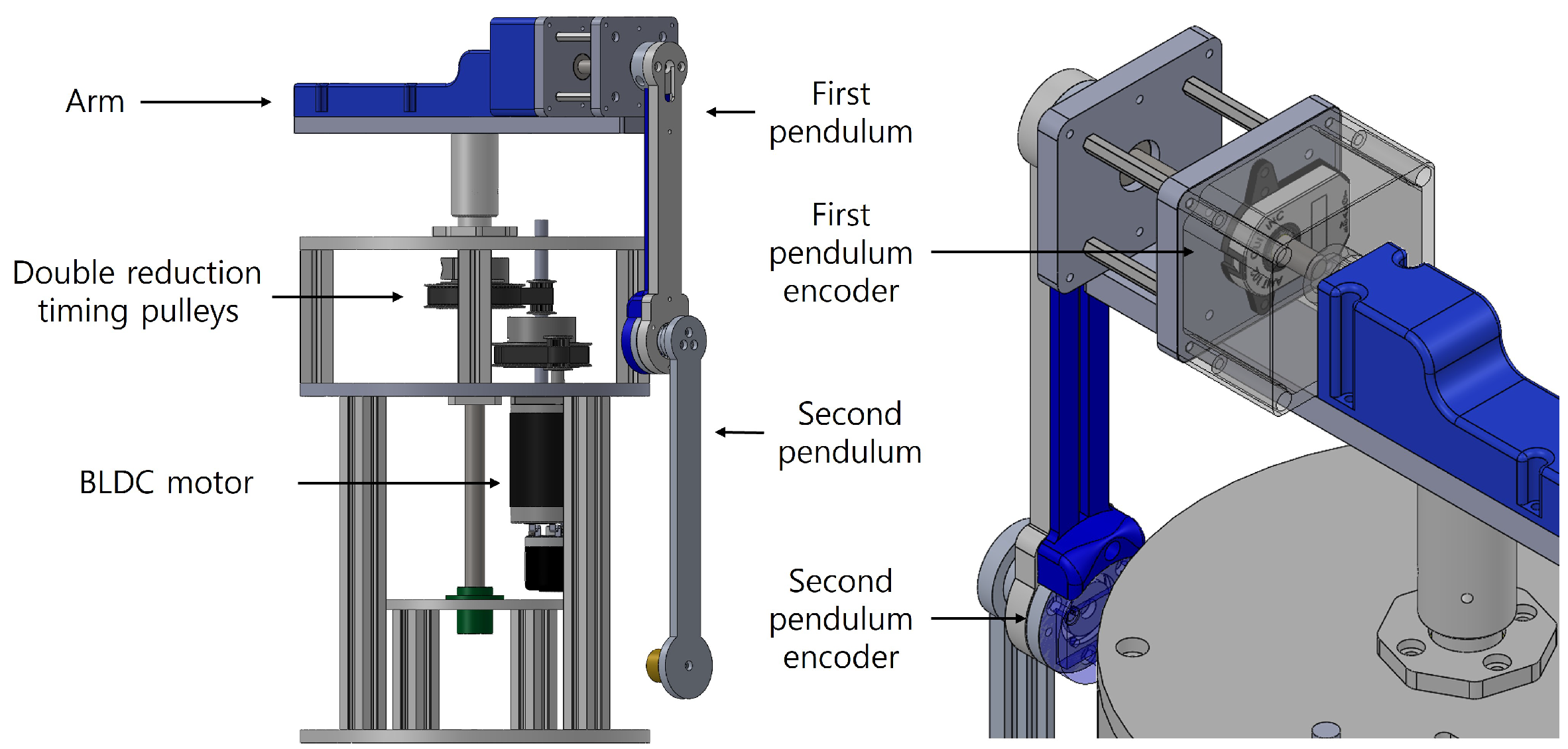
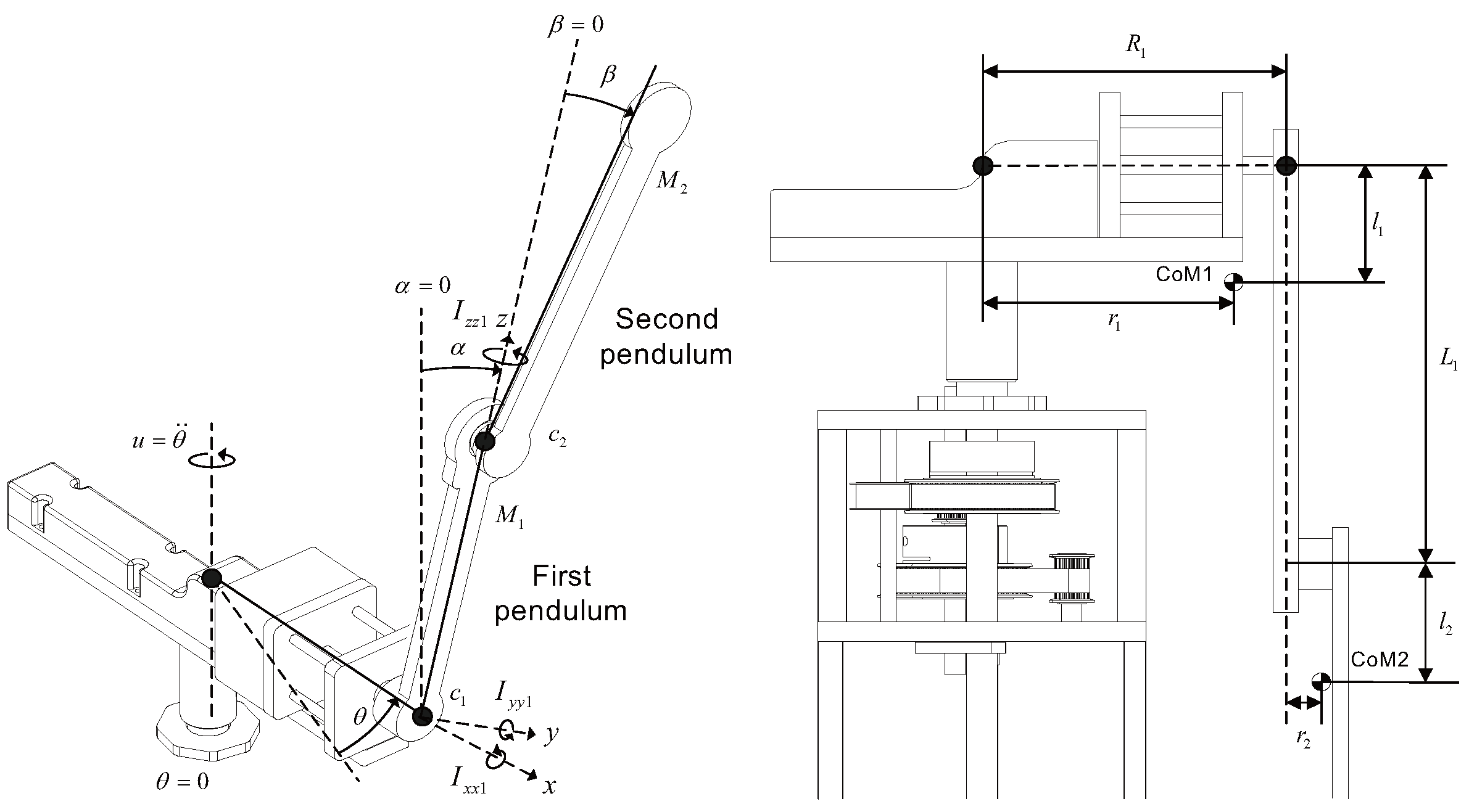
2. System Modeling and Parameter Identification

Figure 1 shows the rotary double-inverted pendulum (RDIP) developed in the authors’ laboratory. The RDIP system is a high-degree-of-freedom nonlinear structure consisting of a horizontally rotating arm and two pendulums connected in series. The arm was actuated by an 80 W brushless DC (BLDC) motor (D&J WITH, Seoul, Republic of Korea), and its angular position and velocity were measured using an E40H8-5000-3-N-5 encoder (Autonics, Mundelein, IL, USA) with a resolution of 20,000 counts per revolution (CPR). For the pendulums, an AMT102-V encoder (Same Sky, Lake Oswego, OR, USA) with a resolution of 8192 CPR was mounted on the first pendulum, while an AS5145B magnetic encoder (ams OSRAM, Premstätten, Austria) with 4096 CPR was used on the second pendulum. These sensors were selected to meet the precision measurement requirements essential for accurate dynamic modeling. A double-reduction transmission system, composed of timing belts and pulleys, was implemented in the motor drive mechanism. Two sequential stages with a 4:1 reduction yielded a total gear ratio of 16:1. This configuration effectively suppresses backlash and enhances precision in angular velocity control, especially when combined with high-resolution encoders. Moreover, the setup enables stable high-torque output, which contributes to maintaining control stability in nonlinear, multi-stage pendulum dynamics. To ensure modeling accuracy and structural consistency, the mechanical system was precisely designed using SolidWorks 2024 in a 3D CAD environment. Geometric symmetry and alignment accuracy were prioritized during the design phase and consistently maintained during physical fabrication to align with the intended specifications. The center of mass (CoM) of each component was carefully calculated based on material properties and mass distribution to minimize dynamic mismatches between the theoretical model and the physical system.

For real-time control and data acquisition, a custom-developed Light-weight Rapid Control Prototyping (LW-RCP) system [29] was employed. This system provides a synchronized interface for both implementing control algorithms on physical hardware and collecting sensor feedback in real-time. To ensure precise synchronization among sensing, computation, and actuation, the control loop was executed with a sampling period of 1 ms. This was realized using MATLAB (2022b) and Simulink (10.6) in a real-time processing environment, enabling periodic and stable control execution. The architecture was specifically designed to suppress the control instability arising from timing discrepancies, ensuring reliable real-time performance throughout the experiment. Additionally, a customized version of the BOOSTXL-DRV8301 inverter board from Texas Instruments was utilized to drive the BLDC motor.

2.1. Dynamic Modeling

In this study, all variables and parameters were defined based on the International System of Units (SI units). Figure 2 illustrates the geometric configuration and physical parameters required for dynamic modeling of the rotary double-inverted pendulum system. The diagram includes an enlarged view of the arm and pendulums, as well as a side view of the entire system. The variable $\theta$ denotes the rotational displacement of the arm from its initial position, while the control input u corresponds to the angular acceleration applied to the arm. The variable $\alpha$ represents the relative angle between the first pendulum and the vertical axis (ground normal), and $\beta$ denotes the relative angular displacement between the second and the first pendulum. $M_1$ and $M_2$ denote the masses of the first and second pendulums, respectively, and CoM1 and CoM2 indicate their respective centers of mass. The distance parameters $L_1$, $l_1$, $l_2$, $R_1$, $r_1$, and $r_2$ are defined as the link lengths and the distances to each pendulum’s center of mass, which are visually represented in the side view in the figure. The rotational friction coefficients at the joints of the first and second pendulums are denoted by $c_1$ and $c_2$, respectively. For the inertia tensor I, terms such as $I_{xx1}$ and $I_{xx2}$ represent the moments of inertia along the x-axis for the first and second pendulums, respectively, while $I_{xz1}$ and $I_{xz2}$ correspond to the cross-inertia components. These inertia properties are incorporated into the system’s dynamic modeling equations.

The dynamic model of the rotary double inverted pendulum system can be derived using the Euler–Lagrange formulation as follows:

$$\begin{array}{c}\hfill \left[\begin{array}{c}{n}_1\\ n_2\end{array}\right]\ddot{\theta }+\left[\begin{array}{cc}{m}_{11}& m_{12}\\ m_{21}& m_{22}\end{array}\right]\left[\begin{array}{c}\ddot{\alpha }\\ \ddot{\beta }\end{array}\right]+\left[\begin{array}{c}{d}_1\\ d_2\end{array}\right]=0\end{array}$$

(1)

Each component of Equation (1) is defined as follows:   

$$\begin{array}{cc}\hfill n_1& =h_{1}cos\left(\alpha \right)+h_{2}cos(\alpha +\beta ),\hfill \\ \hfill n_2& =h_{2}cos(\alpha +\beta ),\hfill \\ \hfill m_{11}& =h_3+h_6+2h_{4}cos\left(\beta \right),\hfill \\ \hfill m_{12}& =h_6+h_{4}cos\left(\beta \right),\hfill \\ \hfill m_{21}& =h_6+h_{4}cos\left(\beta \right),\hfill \\ \hfill m_{22}& =h_6,\hfill \\ \hfill d_1& =-h_{4}sin\beta (2\dot{\alpha }\dot{\beta }+{\dot{\beta }}^2)-h_{5}sin\alpha -h_{7}sin(\alpha +\beta )+c_1\dot{\alpha }\hfill \\ \hfill & -{\dot{\theta }}^2\{{\displaystyle \frac{1}{2}}{h}_{8}sin\left(2\alpha \right)+h_{4}sin(2\alpha +\beta )+{\displaystyle \frac{1}{2}}{h}_{9}sin(2\alpha +2\beta )\},\hfill \\ \hfill d_2& =h_{4}sin\beta \left({\dot{\alpha }}^2\right)-h_{7}sin(\alpha +\beta )+c_2\dot{\beta }\hfill \\ \hfill & -{\dot{\theta }}^2\{{\displaystyle \frac{1}{2}}{h}_{9}sin(2\alpha +2\beta )+{\displaystyle \frac{1}{2}}{h}_4(sin(2\alpha +2\beta )-sin\beta )\}.\hfill \end{array}$$

(2)

The terms in Equation (2) are expressed using the parameters $h_1$ through $h_9$, which are defined in Equation (3). Here, g denotes the gravitational acceleration (9.81 m/s²).

$$\begin{array}{ccc}\hfill h_1& =& M_1{l}_1{r}_1+M_2{L}_1(R_1+r_2)-I_{xz1},\hfill \\ \hfill h_2& =& M_2{l}_2(R_1+r_2)-I_{xz2},\hfill \\ \hfill h_3& =& I_{xx1}+M_1{l}_1^2+M_2{L}_1^2,\hfill \\ \hfill h_4& =& M_2{L}_1{l}_2,\hfill \\ \hfill h_5& =& g(M_1{l}_1+M_2{L}_1),\hfill \\ \hfill h_6& =& I_{xx2}+M_2{l}_2^2,\hfill \\ \hfill h_7& =& M_{2}g{l}_2,\hfill \\ \hfill h_8& =& M_1{l}_1^2+M_2{L}_1^2+I_{yy1}-I_{zz1},\hfill \\ \hfill h_9& =& M_2{l}_2^2+I_{yy2}-I_{zz2}.\hfill \end{array}$$

(3)

Rewriting Equation (1), the angular accelerations of the pendulums are compactly represented in matrix form in Equation (4).

$$\left[\begin{array}{c}\ddot{\alpha }\\ \ddot{\beta }\end{array}\right]=-{\left[\begin{array}{cc}{m}_{11}& m_{12}\\ m_{21}& m_{22}\end{array}\right]}^{-1}\left\{\left[\begin{array}{c}{n}_1\\ n_2\end{array}\right]\ddot{\theta }+\left[\begin{array}{c}{d}_1\\ d_2\end{array}\right]\right\}.$$

(4)

The matrix-form expression for the angular accelerations in Equation (4) can be expanded into scalar form as shown in Equation (5).

$$\begin{array}{ccc}\hfill \ddot{\alpha }& =& {\displaystyle \frac{(-m_{22}{n}_1+m_{12}{n}_2)\ddot{\theta }+(-m_{22}{d}_1+m_{12}{d}_2)}{\mathrm{\Phi }}},\hfill \\ \hfill \ddot{\beta }& =& {\displaystyle \frac{(m_{21}{n}_1-m_{11}{n}_2)\ddot{\theta }+(m_{21}{d}_1-m_{11}{d}_2)}{\mathrm{\Phi }}},\hfill \\ \hfill \mathrm{\Phi }& =& m_{11}{m}_{22}-m_{12}{m}_{21}.\hfill \end{array}$$

(5)

The state vector is defined as $x_1=\theta$, $x_2=\alpha$, $x_3=\beta$, $x_4=\dot{\theta }$, $x_5=\dot{\alpha }$, and $x_6=\dot{\beta }$, with the control input u corresponding to the angular acceleration $\ddot{\theta }$ of the arm. The final nonlinear state-space representation is expressed as follows:   

$$\underset{\dot{x}}{\underbrace{\left[\begin{array}{c}{\dot{x}}_1\\ {\dot{x}}_2\\ {\dot{x}}_3\\ {\dot{x}}_4\\ {\dot{x}}_5\\ {\dot{x}}_6\end{array}\right]}}=\underset{f(x,u)}{\underbrace{\left[\begin{array}{c}{x}_4\\ x_5\\ x_6\\ u\\ {\displaystyle \frac{(-m_{22}{n}_1+m_{12}{n}_2)u+(-m_{22}{d}_1+m_{12}{d}_2)}{\mathrm{\Phi }}}\\ {\displaystyle \frac{(m_{21}{n}_1-m_{11}{n}_2)u+(m_{21}{d}_1-m_{11}{d}_2)}{\mathrm{\Phi }}}\end{array}\right]}}$$

(6)

This derived dynamic model, represented in Equation (6), was implemented as the simulation environment for reinforcement learning training in this study.

2.2. Parameter Identification

To enable sim-to-real reinforcement learning, the accurate identification of system parameters is essential. As illustrated in Figure 2, the physical parameters to be estimated include $M_1$, $M_2$, $I_{xx1}$, $I_{xx2}$, $I_{yy1}$, $I_{yy2}$, $I_{zz1}$, $I_{zz2}$, $I_{xz1}$, $I_{xz2}$, $l_1$, $l_2$, $c_1$, $c_2$, and $L_1$. Among these, parameters such as $M_1$, $M_2$, $I_{xx1}$, $I_{xx2}$, $l_1$, $l_2$, $c_1$, and $c_2$ can be experimentally estimated through trajectory matching. Specifically, by applying a patterned motion to the arm of the rotary pendulum, the first and second pendulums are allowed to swing freely, and their dynamic responses (angles, angular velocities, etc.) are recorded. Then, the system parameters are optimized to minimize the error between the measured trajectories and model simulation outputs. It should be noted that a unique set of parameters may not be guaranteed, as multiple combinations could produce similar trajectories. To illustrate this issue, we consider a simplified single-inverted pendulum (SIP) model with the second pendulum removed. The SIP model can be expressed as

$$\ddot{\alpha }={\zeta }_{1}sin\alpha -{\zeta }_2\dot{\alpha }-{\displaystyle \frac{{\zeta }_1}{g}}cos\alpha u.$$

(7)

where the coefficients ${\zeta }_1$ and ${\zeta }_2$ are defined as:

$${\zeta }_1={\displaystyle \frac{mg{l}_1}{I_{xx1}+m_1{l}_1^2}},{\zeta }_2={\displaystyle \frac{c_1}{I_{xx1}+m_1{l}_1^2}}.$$

(8)

Given that ${\zeta }_1$ and ${\zeta }_2$ are functions of four interrelated parameters, their values alone are insufficient to uniquely determine $I_{xx1}$ and $c_1$ unless additional constraints are imposed. However, $m_1$ and $l_1$ can be directly measured using a scale and a length-measuring device, respectively. By fixing these two values, the remaining parameters, $I_{xx1}$ and $c_1$, become uniquely identifiable. To estimate these, we collected angular position data using the LW-RCP system and numerically approximated the angular acceleration $\ddot{\alpha }$ via the central difference method. Starting from the simplified SIP model in Equation (7), the expression is reformulated as

$$\ddot{\alpha }=\left[sin\alpha -{\displaystyle \frac{1}{g}}cos\alpha u\dot{\alpha }\right]\left[\begin{array}{c}{\zeta }_1\\ {\zeta }_2\end{array}\right]$$

(9)

Assuming data from $t_1$ to $t_N$ is available, the least squares solution is obtained as

$$\begin{array}{c}\hfill \underset{=X}{\underbrace{\left[\begin{array}{c}\ddot{\alpha }\left(t_1\right)\\ \ddot{\alpha }\left(t_2\right)\\ ⋮\\ \dot{\alpha }\left(t_N\right)\end{array}\right]}}=\underset{=Y}{\underbrace{\left[\begin{array}{cc}sin\alpha \left(t_1\right)-{\displaystyle \frac{1}{g}}cos\alpha \left(t_1\right)u\left(t_1\right)& \dot{\alpha }\left(t_1\right)\\ sin\alpha \left(t_2\right)-{\displaystyle \frac{1}{g}}cos\alpha \left(t_2\right)u\left(t_2\right)& \dot{\alpha }\left(t_2\right)\\ ⋮& ⋮\\ sin\alpha \left(t_n\right)-{\displaystyle \frac{1}{g}}cos\alpha \left(t_n\right)u\left(t_n\right)& \dot{\alpha }\left(t_n\right)\end{array}\right]}}\left[\begin{array}{c}{\zeta }_1\\ {\zeta }_2\end{array}\right]\end{array}$$

(10)

The identified coefficients ${\widehat{\zeta }}_1$, ${\widehat{\zeta }}_2$ are computed as

$$\left[\begin{array}{c}{\widehat{\zeta }}_1{\widehat{\zeta }}_2\end{array}\right]={\left(Y^{T}Y\right)}^{-1}{Y}^{T}X$$

(11)

From these, the moment of inertia and damping coefficient are derived as

$$I_{xx1}={\displaystyle \frac{mg{l}_1}{{\widehat{\zeta }}_1}}-m_1{l}_1^2,c_1=(I_{xx1}+m_1{l}_1^2){\widehat{\zeta }}_2$$

(12)

The same procedure is applied for the second pendulum. While $m_2$ and $l_2$ were directly measured, $I_{xx2}$ and $c_2$ were estimated using experimental data. Due to the system’s multi-body nonlinear nature, the accurate representation of the inertial effects requires the full definition of the inertia tensor. This includes not only the principal moments ($I_{xx},I_{yy},I_{zz}$) but also the cross-product terms such as $I_{xz}$. In this study, the inertia tensor was computed using two complementary methods: (1) generating 3D CAD models of each pendulum and calculating the inertia properties based on the mass distribution and CoM; (2) refining these initial values via experimental tuning using the MATLAB’s fmincon optimization. The optimization process minimizes the mean squared error (MSE) between model output and real-world data while imposing physical constraints on the parameters. The bounds for each parameter were selected based on hardware specifications, prior CAD measurements, and physically plausible ranges to ensure meaningful and realistic results. The specific lower and upper bounds used during the fmincon optimization are summarized in

Table 1. Parameter bounds used for constrained optimization in fmincon.

Parameter	Lower Bound (Min)	Upper Bound (Max)
$M_1,M_2$	$M_1,M_2$	$M_1,M_2$
$I_{xx1},I_{yy1},I_{zz1},I_{xz1}$	0	$1\times {10}^{-2}$
$I_{xx2},I_{yy2},I_{zz2},I_{xz2}$	0	$1\times {10}^{-2}$
$c_1,c_2$	$3\times {10}^{-7}$	$1\times {10}^{-4}$
$l_1,l_2$	$l_1,l_2$	$l_1,l_2$
$r_1,r_2$	$r_1,r_2$	$r_1,r_2$

.

This hybrid approach allows the precise identification of key parameters including mass, moment of inertia, CoM distance, and damping coefficients. The final estimated parameters used in this study are listed in

Table 2. Summary of the parameters for the rotary double-inverted pendulum.

Parameter	Value
$M_1$	0.187 kg
$M_2$	0.132 kg
$I_{xx1}$	1.0415 × ${10}^{-3}$ kgm2
$I_{xx2}$	8.8210 × ${10}^{-4}$ kgm2
$I_{yy1}$	4.3569 × ${10}^{-3}$ kgm2
$I_{yy2}$	4.9793 × ${10}^{-3}$ kgm2
$I_{zz1}$	3.3179 × ${10}^{-3}$ kgm2
$I_{zz2}$	4.8178 × ${10}^{-3}$ kgm2
$I_{xz1}$	3.7770 × ${10}^{-4}$ kgm2
$I_{xz2}$	1.9823 × ${10}^{-4}$ kgm2
$l_1$	0.072 m
$l_2$	0.133 m
$c_1$	2.4100 × ${10}^{-6}$
$c_2$	1.0900 × ${10}^{-6}$
$L_1$	0.1645 m
$R_1$	0.1625 m
$r_1$	0.1597 m
$r_2$	0.0209 m

. To enhance the clarity of Table 2, we briefly summarize the physical significance of each parameter. The parameters $M_1$ and $M_2$ represent the masses of the first and second pendulums, respectively. The terms $I_{xx},I_{yy},I_{zz},I_{xz}$ correspond to the components of the inertia tensor for both pendulums, encompassing both principal moments of inertia and cross-moments. The parameters $l_1,r_1,l_2,$ and $r_2$ indicate the vertical and horizontal distances from the rotation axis to the center of mass of the first and second pendulums. Specifically, the pairs $(l_1,r_1)$ and $(l_2,r_2)$ describe the center-of-mass positions in both the vertical and horizontal directions. The parameter $L_1$ denotes the distance from the rotation axis of the first pendulum to the rotation axis of the second pendulum, while $R_1$ represents the horizontal distance from the central rotation axis to the pivot point of the first pendulum.

To validate the physical consistency of the identified parameters, an open-loop experiment was conducted. As shown in Figure 3, a 2 s sine wave input was applied to the arm, and the resulting $\alpha$ and $\beta$ trajectories were compared between the simulation model (dashed lines) and the actual system (solid lines). Although the simulation output was not identical to the experimental data, the overall patterns and response dynamics matched closely, indicating that the derived mathematical model effectively captured the real system’s dynamics.

3. Reinforcement-Learning-Based Simulation

This paper is based on the transition control problem formulated in previous work [6], aiming to achieve robust transition control under disturbance conditions that are difficult to address using conventional approaches through sim-to-real reinforcement learning. While prior research relied on precomputed trajectories and controllers derived via offline optimization, the present work proposes a reinforcement-learning-based control policy that can perform stable transition control in real time, even under various external disturbances, through iterative learning. The reinforcement learning agent interacts with an environment implemented in Python (3.9.13), which was constructed using the dynamic model equations introduced in Section 2. Unlike prior model-free approaches that often suffer from instability in real-world deployment, as reported in recent studies [27,28], the proposed method leverages a physically consistent model calibrated through experimental parameter estimation. This enables robust transition control across four distinct equilibrium configurations—an advancement over earlier works that focused solely on single-point stabilization. Similar benefits of incorporating accurate actuator models and system identification into reinforcement learning pipelines have been demonstrated in sim-to-real studies for rough-terrain vehicles [24] and broader robotic systems [30].

3.1. Training Environment

The physical parameters used to construct the simulation environment for the rotary double-inverted pendulum are listed in Table 2. The simulation solved the system’s nonlinear ordinary differential equations using the ode4 Runge–Kutta method. After training was completed in the Python-based environment, the learned policy was converted into a MATLAB/Simulink-compatible format using the matlab.engine module provided by MATLAB, enabling its direct deployment within a real-time control system. The converted parameter values served as key components in configuring the reinforcement-learning-based controller. In the simulation, each episode lasted 10 s. The internal dynamics were updated in a 1 ms interval, while the agent observed the environment every 10 ms. Accordingly, the agent interacted with the environment up to 1000 times per episode, and its policy was improved incrementally based on the reward feedback at each time step. The observable state vector in the simulation environment was defined by the system’s nonlinear dynamics, as formulated in Section 2, and consisted of the variables $\theta$, $\alpha$, $\beta$, $\dot{\theta }$, $\dot{\alpha }$, and $\dot{\beta }$. To ensure stable reward computation, the angular variables $\theta$, $\alpha$, and $\beta$ were wrapped to the range $[-\pi ,\pi ]$ using modular arithmetic. For enhanced continuity and normalization during training, the angular states were reparameterized using sine and cosine transformations. The final state vector perceived by the agent is defined as

$$\begin{array}{c}\hfill s_t=[sin\left(\theta \right),cos\left(\theta \right),sin\left(\alpha \right),cos\left(\alpha \right),sin\left(\beta \right),cos\left(\beta \right),\dot{\theta },\dot{\alpha },\dot{\beta },\mathrm{EP}].\end{array}$$

(13)

Here, EP represents a contextual variable denoting the target equilibrium point for transition control. Each equilibrium configuration corresponds to a binary combination of pendulum orientations, with the first and second pendulums encoded as either 1 (Up) or 0 (Down). For instance, EP0 denotes (Down-Down), EP1 denotes (Down-Up), EP2 denotes (Up-Down), and EP3 denotes (Up-Up). This representation enables the agent to interpret multiple equilibrium transition tasks under a unified learning framework and adapt its control actions according to the current target. The control output of the agent is a continuous input $u\in [-50,50]$, representing the angular acceleration applied to the motor. Given the current state $s_t$, the agent generates the control command via its learned policy ${\pi }_{\theta }$ as follows:

$$\begin{array}{c}\hfill u\left(t\right)={\pi }_{\theta }\left(s_t\right).\end{array}$$

(14)

The reward function was designed to guide the agent toward reaching the designated equilibrium point while penalizing physical constraint violations and terminating the episode in cases of failure within a specified time limit. This framework enables the agent to develop a robust transition control strategy without relying on pre-computed trajectories or model-based controllers, even under diverse initial conditions.

3.2. Learning Algorithm

In this study, a reinforcement-learning-based policy was trained to perform transition control among four equilibrium configurations of the rotary double-inverted pendulum system. The training setup employed an off-policy structure capable of handling continuous state and action spaces. The simulation environment was constructed in MATLAB/Simulink based on the nonlinear dynamic model derived in the previous section, while the learning algorithm itself was developed in Python. The algorithm used in this work was Truncated Quantile Critics (TQC) [31], which combines the Soft Actor–Critic (SAC) [32] method with the distributional value estimation approach of Quantile Regression Deep Q-Network (QR-DQN) [33]. TQC suppresses overestimation bias by truncating the upper quantiles of the Q-value distribution, allowing for more stable value predictions and policy updates. This makes it particularly effective for nonlinear and high-dimensional systems such as the rotary double-inverted pendulum, as it improves the stability and convergence rate of the learning process. To enhance robustness across various transition scenarios, the algorithm uses multiple critics, which improves the generalization capability of the policy. In order to reduce overall training time, fewer critic networks were used, while the policy network was expanded to learn the transitions between all four equilibrium points within a single model. All other hyperparameters followed the default settings provided in the original TQC paper [31].

3.3. Training Settings

3.3.1. Experimental Environment

The reinforcement learning training was conducted on a Windows-based system equipped with an Intel Core i5-11400 CPU and 32 GB of RAM and ran for approximately 5 million time steps, taking about 2.4 days to complete. Each episode began from a randomly sampled initial condition, and the control mode EP (equilibrium point) was changed every episode to ensure that the policy could learn the transitions between all four equilibrium points. The initial states were uniformly sampled within the following ranges, which reflect the operating limits of the physical system:

$$\begin{array}{ccc}\hfill \theta ,\alpha ,\beta & \sim & \hfill \mathcal{U}(-\pi ,\pi ),\hfill \\ \hfill \dot{\theta }& \sim & \hfill \mathcal{U}(-7,7),\hfill \\ \hfill \dot{\alpha }& \sim & \hfill \mathcal{U}(-10,10),\hfill \\ \hfill \dot{\beta }& \sim & \hfill \mathcal{U}(-20,20).\hfill \end{array}$$

(15)

Although this random initialization may generate unrealistic combinations of states in the early stages of training, such states are only encountered in simulation and do not affect the deployment of the policy on the physical system. This setting encourages the agent to learn recovery properties under diverse conditions, and the corresponding results are discussed in the next section.

3.3.2. Reward Function

The reward function provides feedback for each action taken by the agent, reflecting whether the target equilibrium is reached and the efficiency of control input. For the rotary double-inverted pendulum, each equilibrium configuration is defined by a control mode EP, which determines the target angles ${\alpha }^{*}$ and ${\beta }^{*}$.

Table 3. Target angles for the first and second pendulums corresponding to each target equilibrium point.

Equilibrium Point (EP)	Target Angle
	${\mathbf{\alpha }}^{*}$	${\mathbf{\beta }}^{*}$
0	−$\pi$	0
1	−$\pi$	−$\pi$
2	0	−$\pi$
3	0	0

shows the target angles for each equilibrium point.

The total reward is computed as the product of the following components:

$$\begin{array}{ccc}\hfill R_u& =& exp(-0.005|u\left|\right),\hfill \\ \hfill R_{\theta }& =& 0.5+0.5\times cos\left(\theta \right),\hfill \\ \hfill R_{\alpha }& =& 0.5+0.5\times cos(\alpha -{\alpha }^{*}),\hfill \\ \hfill R_{\beta }& =& 0.5+0.5\times cos(\beta -{\beta }^{*}),\hfill \\ \hfill R_{\dot{\theta }}& =& exp(-0.02|\dot{\theta }\left|\right),\hfill \\ \hfill R_{\dot{\alpha }}& =& exp(-0.02|\dot{\alpha }\left|\right),\hfill \\ \hfill R_{\dot{\beta }}& =& exp(-0.02|\dot{\beta }\left|\right),\hfill \\ \hfill \mathrm{Reward}& =& R_u\times R_{\theta }\times R_{\alpha }\times R_{\beta }\times R_{\dot{\theta }}\times R_{\dot{\alpha }}\times R_{\dot{\beta }}.\hfill \end{array}$$

(16)

This structure was designed to simultaneously encourage energy-efficient control, angular and velocity stability, and accurate convergence to the target configuration. Figure 4 and Figure 5 visualize the individual components of the reward function.

Figure 6 shows the reward convergence curve throughout the reinforcement learning process. The graph presents the average reward over every 10 episodes, highlighting the overall convergence behavior. In this study, training was conducted for a total of 5 million steps, with reward values stabilizing around 1 million steps. Training was terminated when an average reward of 897 was reached, taking approximately 2.4 days. The model used in the real-world experiment was obtained around the 2 million step mark (day 1) and also achieved an average reward of 897. As noted earlier, the agent could interact with the environment up to 1000 times per episode, accumulating rewards at each time step. Thus, the theoretical maximum episode reward was 1000, indicating that the system perfectly maintained the desired equilibrium throughout the entire episode. The average reward of 897 achieved in this study suggested that the agent maintained stable configurations most of the time, demonstrating effective control. These results validate that the proposed reward function design and policy learning strategy effectively minimize control effort, stabilize angular states, and ensure accurate convergence to the target equilibrium.

4. Reinforcement-Learning-Based Transition Control Using Sim-to-Real Transfer

4.1. Simulation

Prior to deploying the trained policy on the actual controller, a simulation was conducted in Simulink by integrating the rotary double-inverted pendulum model based on the Euler–Lagrange formulation described in Section 2 with the trained reinforcement learning policy. This simulation aimed to pre-validate whether the learned policy could operate stably under conditions closely resembling those of the physical system and to assess the transition stability of the reinforcement-learning-based controller. The trained policy was embedded into the controller block within Simulink, and a transition control scenario was simulated, initiating from the equilibrium configuration EP0 and targeting EP3. The simulation was executed at a sampling interval of 1 ms, matching the real system’s control rate, and the results were analyzed focusing on the pendulum angle trajectories, the arm velocity profiles of the control input, and the success of reaching the target equilibrium point. Figure 7 shows the velocity control input applied to the arm, along with the angular trajectories of the first and second pendulums during the transition from EP0 to EP3. These results confirm that the learned policy effectively performs a stable swing-up motion even within the physical model, successfully reaching the target equilibrium state while maintaining overall system stability.

4.2. Experiment

To initiate the evaluation of real-world performance, a comparative swing-up experiment was first conducted to assess the recovery characteristics of the proposed RL-based controller against the conventional two-degree-of-freedom (2-DOF) method [6]. Both controllers performed a transition from the downward equilibrium (EP0) to the upright configuration (EP3), during which a strong external disturbance was applied. As shown in Figure 8, the RL-based controller (right) quickly stabilized the system by leveraging its learned policy. The green dotted line in each subplot denotes the moment at which the external disturbance was applied. In contrast, the 2-DOF method (left) failed to recover, not only due to limitations in its precomputed feedforward trajectory but also because the control command generated exceeded the physical velocity limit of the arm, triggering the system’s protection mechanism and halting further control. This result highlights the adaptive robustness of the RL-based controller in the presence of unforeseen perturbations and its superior compatibility with real-world hardware constraints.

To evaluate the sim-to-real performance of the trained policy, transition control experiments were conducted on the rotary double-inverted pendulum system across four stable equilibrium points. Each equilibrium configuration corresponded to one of four possible modes ($\mathrm{EP}\in 0,1,2,3$), defined based on the combinatorial orientation of the two pendulums. Transitions between these modes were executed sequentially to validate the completeness of the training, and disturbances were intentionally introduced at each stable configuration to assess the policy’s recovery properties. Specifically, transitions occurred in the following time windows: EP0 from 0 to 15 s, EP1 from 16 to 30 s, EP2 from 31 to 45 s, and EP3 from 46 to 60 s, concluding with a return to EP0. The green dotted line in the result plots indicates the moment when a disturbance was applied during the experiment. The experimental results demonstrated that the agent consistently returned to the desired mode even after disturbances and maintained robust and stable control performance across all transition scenarios.

These findings experimentally confirm that the reinforcement-learning-based controller exhibits strong recovery properties and high adaptability on the physical system. Notably, in contrast to conventional two-degree-of-freedom control approaches that rely on precomputed trajectories, the proposed method computes control inputs in real time based on the current state, achieving reliable performance under diverse initial conditions and external perturbations. The experimental results are visualized in Figure 9, which illustrates the trajectories and recovery properties across different equilibrium modes. Additionally, Figure 10 presents a captured frame from the full experimental video, which is available on the laboratory’s YouTube channel at https://youtu.be/dgg2hHUqvck (accessed on 17 May 2025), allowing for intuitive observation of the transition and recovery properties on the real hardware. While we do not provide a direct numerical benchmark due to differences in experimental setups and control objectives across the literature, we emphasize a key comparative insight: most existing reinforcement learning controllers for rotary pendulum systems—particularly those using model-free strategies—focus solely on swing-up or stabilization at a single equilibrium point and often fail under external disturbances or multiple target modes. In contrast, our policy demonstrates reliable real-time transition and robust recovery across all four configurations in both simulation and real-world experiments. This highlights a meaningful expansion in control capability that, to the best of our knowledge, has not been acheived in prior work.

5. Conclusions

In this study, a sim-to-real reinforcement learning approach was proposed and implemented to achieve transition control and disturbance recovery across four equilibrium configurations of a rotary double-inverted pendulum system. A simulation environment was constructed based on precise parameter identification and mathematical modeling, and a reinforcement learning policy was trained within this framework before being directly deployed on the physical system. High-resolution sensor data were used to accurately estimate the key dynamic parameters, and the resulting mathematical model served as the learning environment for the reinforcement learning agent. The Truncated Quantile Critics (TQC) algorithm was employed as the learning method, effectively enabling the agent to acquire a generalized policy capable of handling a wide range of initial conditions and equilibrium transitions. Without any additional tuning or calibration, the trained policy was applied directly to the real system and demonstrated robust performance across all four equilibrium transitions and recovery tests. These results indicate that, beyond the limitations of trajectory-based controllers, real-time policies derived from reinforcement learning can achieve robust control performance even in high-dimensional nonlinear systems. The methodology presented in this study offers practical applicability for sim-to-real control research on complex systems such as the rotary inverted pendulum and is expected to contribute foundational insights for future deployment in broader robotic control scenarios.

References

1. Izutsu, M.; Pan, Y.; Furuta, K. Swing-up of Furuta Pendulum by Nonlinear Sliding Mode Control. Sice J. Control Meas. Syst. Integr. 2008, 1, 12–17. [Google Scholar] [CrossRef]
2. Glück, T.; Eder, A.; Kugi, A. Swing-up control of a triple pendulum on a cart with experimental validation. Automatica 2013, 49, 801–808. [Google Scholar] [CrossRef]
3. Rigatos, G.; Abbaszadeh, M.; Siano, P.; Cuccurullo, G.; Pomares, J.; Sari, B. Nonlinear Optimal Control for the Rotary Double Inverted Pendulum. Adv. Control Appl. 2024, 6, e140. [Google Scholar] [CrossRef]
4. Zied, B.H.; Mohammad, J.F.; Zafer, B. Development of a Fuzzy-LQR and Fuzzy-LQG stability control for a double link rotary inverted pendulum. J. Frankl. Inst. 2020, 357, 10529–10556. [Google Scholar]
5. Graichen, K.; Treuer, M.; Zeitz, M. Swing-up of the double pendulum on a cart by feedforward and feedback control with experimental validation. Automatica 2007, 43, 63–71. [Google Scholar] [CrossRef]
6. Ju, D.; Lee, T.; Lee, Y.S. Transition Control of a Rotary Double Inverted Pendulum Using Direct Collocation. Mathematics 2025, 13, 640. [Google Scholar] [CrossRef]
7. Turcato, N.; Calì, M.; Dalla Libera, A.; Giacomuzzo, G.; Carli, R.; Romeres, D. Learning Global Control of Underactuated Systems with Model-Based Reinforcement Learning. arXiv 2025, arXiv:2504.06721. [Google Scholar]
8. Taets, J.; Lefebvre, T.; Ostyn, F.; Crevecoeur, G. Energy-Based Exploration for Reinforcement Learning of Underactuated Mechanical Systems. IEEE Access 2025, 13, 98847–98859. [Google Scholar] [CrossRef]
9. Kormushev, P.; Calinon, S.; Saegusa, R.; Metta, G. Learning the skill of archery by a humanoid robot iCub. In Proceedings of the 2010 10th IEEE—RAS International Conference on Humanoid Robots, Nashville, TN, USA, 6–8 December 2010; pp. 417–423. [Google Scholar]
10. Kormushev, P.; Calinon, S.; Caldwell, D.G. Reinforcement Learning in Robotics: Applications and Real-World Challenges. Robotics 2013, 2, 122–148. [Google Scholar] [CrossRef]
11. Haarnoja, T.; Ha, S.; Zhou, A.; Tan, J.; Tucker, G.; Levine, S. Learning to Walk via Deep Reinforcement Learning. arXiv 2019, arXiv:1812.11103. [Google Scholar]
12. Rupam Mahmood, A.; Korenkevych, D.; Komer, B.J.; Bergstra, J. Setting up a Reinforcement Learning Task with a Real-World Robot. In Proceedings of the 2018 IEEE/RSJ International Conference on Intelligent Robots and Systems (IROS), Madrid, Spain, 1–5 October 2018; pp. 4635–4640. [Google Scholar]
13. Sun, C.; Orbik, J.; Devin, C.M.; Yang, B.H.; Gupta, A.; Berseth, G.; Levine, S. Fully Autonomous Real-World Reinforcement Learning with Applications to Mobile Manipulation. In Proceedings of the 5th Conference on Robot Learning; Faust, A., Hsu, D., Neumann, G., Eds.; Publishing PMLR: London, UK, 2021; pp. 308–319. [Google Scholar]
14. Dang, K.N.; Van, L.V. Development of deep reinforcement learning for inverted pendulum. Int. J. Electr. Comput. Eng. 2023, 13, 3895–3902. [Google Scholar]
15. Zhao, W.; Queralta, J.P.; Westerlund, T. Sim-to-Real Transfer in Deep Reinforcement Learning for Robotics: A Survey. In Proceedings of the 2020 IEEE Symposium Series on Computational Intelligence (SSCI), Canberra, ACT, Australia, 1–4 December 2020; pp. 737–744. [Google Scholar]
16. Kalapos, A.; Gór, C.; Moni, R.; Harmati, I. Sim-to-real reinforcement learning applied to end-to-end vehicle control. In Proceedings of the 2020 23rd International Symposium on Measurement and Control in Robotics (ISMCR), Budapest, Hungary, 15–17 October 2020; pp. 1–6. [Google Scholar]
17. Kaspar, M.; Osorio, J.D.M.; Bock, J. Sim2real transfer for reinforcement learning without dynamics randomization. In Proceedings of the 2020 IEEE/RSJ International Conference on Intelligent Robots and Systems (IROS), Las Vegas, NV, USA, 24 October 2020–24 January 2021; pp. 4383–4388. [Google Scholar]
18. Tobin, J.; Fong, R.; Ray, A.; Schneider, J.; Zaremba, W.; Abbeel, P. Domain randomization for transferring deep neural networks from simulation to the real world. In Proceedings of the 2017 IEEE/RSJ International Conference on Intelligent Robots and Systems (IROS), Vancouver, BC, Canada, 24–28 September 2017; pp. 23–30. [Google Scholar]
19. Matas, J.; James, S.; Davison, A.J. Sim-to-real reinforcement learning for deformable object manipulation. In Proceedings of The 2nd Conference on Robot Learning; Billard, A., Dragan, A., Peters, J., Morimoto, J., Eds.; Publishing PMLR: London, UK, 2018; pp. 734–743. [Google Scholar]
20. Arndt, K.; Hazara, M.; Ghadirzadeh, A.; Kyrki, V. Meta Reinforcement Learning for Sim-to-real Domain Adaptation. In Proceedings of the 2020 IEEE International Conference on Robotics and Automation (ICRA), Paris, France, 31 May–31 August 2020; pp. 2725–2731. [Google Scholar]
21. James, S.; Wohlhart, P.; Kalakrishnan, M.; Kalashnikov, D.; Irpan, A.; Ibarz, J.; Levine, S.; Hadsell, R.; Bousmalis, K. Sim-To-Real via Sim-To-Sim: Data-Efficient Robotic Grasping via Randomized-To-Canonical Adaptation Networks. In Proceedings of the IEEE/CVF Conference on Computer Vision and Pattern Recognition (CVPR), 11–15 June 2019; pp. 12627–12637. [Google Scholar]
22. Tong, D.; Choi, A.; Qin, L.; Huang, W.; Joo, J.; Jawed, M.K. Sim2Real Neural Controllers for Physics-Based Robotic Deployment of Deformable Linear Objects. Int. J. Robot. Res. 2023, 6, 791–810. [Google Scholar] [CrossRef]
23. Wang, K.; Johnson, W.R.; Lu, S.; Huang, X.; Booth, J.; Kramer-Bottiglio, R.; Aanjaneya, M.; Bekris, K. Real2Sim2Real Transfer for Control of Cable-Driven Robots Via a Differentiable Physics Engine. In Proceedings of the 2023 IEEE/RSJ International Conference on Intelligent Robots and Systems (IROS), Detroit, MI, USA, 1–5 October 2023; pp. 2534–2541. [Google Scholar]
24. Wiberg, V.; Wallin, E.; FA¨lldin, A.; Semberg, T.; Rossander, M.; Wadbro, E.; Servin, M. Sim-to-real transfer of active suspension control using deep reinforcement learning. Robot. Auton. Syst. 2024, 179, 104731. [Google Scholar] [CrossRef]
25. Rai, A.; Bhushan, B.; Jaint, B. Stabilization and Performance Analysis of Double Link-Rotary Inverted Pendulum Using LQR-I Controller. In Proceedings of the 2025 3rd IEEE International Conference on Industrial Electronics: Developments & Applications (ICIDeA), Bhubaneswar, India, 21–22 February 2025; pp. 1–5. [Google Scholar]
26. Lee, T.; Ju, D.; Lee, Y.S. Transition Control of a Double-Inverted Pendulum System Using Sim2Real Reinforcement Learning. Machines 2025, 13, 186. [Google Scholar] [CrossRef]
27. Bo¨hm, P.; Pounds, P.; Chapman, A.C. Low-cost Real-world Implementation of the Swing-up Pendulum for Deep Reinforcement Learning Experiments. arXiv 2025, arXiv:2503.11065. [Google Scholar]
28. Ho, T.-N.; Nguyen, V.-D.-H. Model-Free Swing-Up and Balance Control of a Rotary Inverted Pendulum Using the TD3 Algorithm: Simulation and Experiments. Eng. Technol. Appl. Sci. Res. 2025, 15, 19316–19323. [Google Scholar] [CrossRef]
29. Lee, Y.S.; Jo, B.; Han, S. A light-weight rapid control prototyping system based on open source hardware. IEEE Access 2017, 5, 11118–11130. [Google Scholar] [CrossRef]
30. Chukwurah, N.; Adebayo, A.S.; Ajayi, O.O. Sim-to-Real Transfer in Robotics: Addressing the Gap Between Simulation and Real-World Performance. Int. J. Robot. Simul. 2024, 6, 89–102. [Google Scholar] [CrossRef]
31. Kuznetsov, A.; Shvechikov, P.; Grishin, A.; Vetrov, D. Controlling overestimation bias with truncated mixture of continuous distributional quantile critics. In Proceedings of the International Conference on Machine Learning, Virtual, 13–18 July 2020; pp. 5556–5566. [Google Scholar]
32. Haarnoja, T.; Zhou, A.; Abbeel, P.; Levine, S. Soft actor-critic: Off-policy maximum entropy deep reinforcement learning with a stochastic actor. In Proceedings of the International Conference on Machine Learning, Stockholm, Sweden, 10–15 July 2018; pp. 1861–1870. [Google Scholar]
33. Dabney, W.; Rowland, M.; Bellemare, M.; Munos, R. Distributional reinforcement learning with quantile regression. In Proceedings of the AAAI Conference on Artificial Intelligence, New Orleans, LA, USA, 2–7 February 2018; Volume 32. [Google Scholar]
Figure 1. Structural diagram of the rotary double-inverted pendulum system developed in laboratory.
Mathematics 13 01996 g001
Figure 2. Geometric and inertial parameters of the rotary double-inverted pendulum system.
Mathematics 13 01996 g002
Figure 3. Open-loop response comparison between the simulation model (dotted line) and the physical system (solid line).
Mathematics 13 01996 g003
Figure 4. Reward function elements: R u , R θ , R θ ˙ , R α ˙ , and R β ˙ .
Mathematics 13 01996 g004
Figure 5. Reward function elements R α and R β dependent on the target equilibrium point (EP).
Mathematics 13 01996 g005
Figure 6. Reward function elements independent of the target equilibrium point.
Mathematics 13 01996 g006
Figure 7. Simulink simulation of transition from EP0 (Down-Down) to EP3 (Up-Up).
Mathematics 13 01996 g007
Figure 8. Disturbance response during swing-up (EP0–EP3). (Left) response of the 2-DOF controller. (Right) response of the RL-based controller.
Mathematics 13 01996 g008
Figure 9. Experimental results of transition control using the RL-based policy, demonstrating recovery properties across four equilibrium configurations.
Mathematics 13 01996 g009
Figure 10. YouTube video recording of the transition control experiment using reinforcement learning.
Mathematics 13 01996 g010