Kernel Ridge-Type Shrinkage Estimators in Partially Linear Regression Models with Correlated Errors

Abstract

Partially linear time series models often suffer from multicollinearity among regressors and autocorrelated errors, both of which can inflate estimation risk. This study introduces a generalized ridge-type kernel (GRTK) framework that combines kernel smoothing with ridge shrinkage and augments it through ordinary and positive-part Stein adjustments. Closed-form expressions and large-sample properties are established, and data-driven criteria—including GCV, AICc, BIC, and RECP—are used to tune the bandwidth and shrinkage penalties. Monte-Carlo simulations indicate that the proposed procedures usually reduce risk relative to existing semiparametric alternatives, particularly when the predictors are strongly correlated and the error process is dependent. An empirical study of US airline-delay data further demonstrates that GRTK produces a stable, interpretable fit, captures a nonlinear air-time effect overlooked by conventional approaches, and leaves only a modest residual autocorrelation. By tackling multicollinearity and autocorrelation within a single, flexible estimator, the GRTK family offers practitioners a practical avenue for more reliable inference in partially linear time series settings.

1. Introduction

In many time series applications, one must balance interpretability and flexibility in the modeling. Partially linear regression models achieve this by expressing the response as a parametric linear function of some covariates alongside a nonparametric smooth function of an additional variable. Specifically, we consider the following model setup:

$$y_t={\mathbf{x}}_t^{\prime }\mathsf{\beta }+f\left(z_t\right)+{\epsilon }_t, t=1,\dots ,n,$$

(1)

where $y_t$ denotes the stationary response at time $t$, and its prediction depends on the p-dimensional vector of explanatory variables ${\mathbf{x}}_t={\left(x_{t1},\dots ,x_{tp}\right)}^{\prime }$ with $x_{t1}={(x_1,\dots ,x_n)}^{\prime }$ and an extra univariate variable $z_t$. Also, $\mathsf{\beta }\in {\mathbb{R}}^p$ is an unknown p-dimensional parameter vector to be estimated, $f\left(.\right)$ is an unknown smooth function, and ${\epsilon }_t’s$ are the error terms.

Unlike classical linear models, (1) offers the interpretability of $\mathsf{\beta }$ while retaining the capacity to model complex, nonlinear effects through $f(.)$ (see [1]). However, two mojor issues often arise:

• Multicollinearity among ${\mathbf{x}}_t.$ When the columns of ${\mathbf{x}}_t$ are nearly linearly dependent, ordinary least squares (OLS) or unpenalized nonparametric estimators can have extremely high variances [2].
• Autocorrelation or dependence among ${\epsilon }_t$, as is common in time series or longitudinal settings. We capture this by a first-order autoregressive process:

  $${\epsilon }_t=\rho {\epsilon }_{t-1}+u_t, \left|\rho \right|<1, u_t~i.i.d. N\left(0,{\sigma }^2\right), t=\mathrm{1,2},\dots ,n$$

  (2)

  ensuring that ${\epsilon }_t$ is stationarily dependent over time ([3,4]). In addition, to simplify the notational illustration, a matrix–vector form of the model (1) can be stated as

  $$\mathbf{y}=\mathbf{X}\mathsf{\beta }+\mathbf{f}+\mathsf{\epsilon },$$

  (3)

  where $\mathbf{y}=\left(y_1,\dots ,y_n\right)$, ${\mathbf{X}=({\mathbf{x}}_1,\dots ,{\mathbf{x}}_n)}^{\prime }$, $\mathbf{f}=\left(f\left(z_1\right),\dots ,f\left(z_n\right)\right)$ and $\mathsf{\epsilon }=\left({\epsilon }_1,\dots ,{\epsilon }_n\right)$. The main goal is to estimate the unknown parameter vector $\mathsf{\beta }$, the smooth function $f\left(t\right)$ and the mean vector $\mathit{\mu }=\mathbf{X}\mathsf{\beta }+\mathbf{f}$ based on the observations from the data set {${ y}_t, {\mathbf{x}}_t{,z}_t$}. Partially linear models enable easier interpretation of the effect of each variable and owing to the “curse of dimensionality”, these models can be preferred to a completely nonparametric regression model. Specifically, partially linear models are more practical than the classical linear model because they combine both the parametric part presented numerically and the nonparametric part displayed graphically.

Even though partially linear models have specific advantages, these models typically assume uncorrelated errors ([1,5]). In real-world time series or panel data, ignoring assumption (2) can degrade efficiency and produce biased inferences ([6,7]). Moreover, multicollinearity among ${\mathbf{x}}_t$ amplifies these problems, inflating variances to the point that $\mathsf{\beta }$ estimates become unreliable ([8,9]).

Despite steady progress on partially linear models, two shortcomings persist. First, kernel-based estimators that handle autocorrelated errors—e.g., efficient GLS-type fits [4] —leave the multicollinearity problem untreated. Second, ridge or Stein-type shrinkage estimators developed for i.i.d. settings ([8,10]) do not accommodate serial dependence. To our knowledge, no existing method tackles collinearity and autocorrelation simultaneously within a single, closed-form estimator; nor do prior studies examine how data-driven criteria jointly tune the kernel bandwidth and shrinkage weight. Filling this gap is the focus of the present work. Accordingly, our objective is to develop and rigorously evaluate a unified estimator that stabilizes the parametric coefficients under multicollinearity, adapts to unknown nonlinear structure, and remains efficient in the presence of autoregressive errors.

To mitigate these issues, we adopt ridge-type kernel smoothing for the parametric component. In essence, a shrinkage penalty is added so that the linear portion $\mathsf{\beta }$ is “shrunk” toward zero to stabilize the estimation. Mathematically, for instance, a ridge-type kernel (RTK) estimator of $\mathsf{\beta }$ can be expressed (after suitable data transformation) as in (6) which has been extensively studied by [11]. This ridge-inspired framework stems from Stein-type shrinkage theory, which shows that biased estimators can dominate unbiased ones, particularly in moderate-to-high dimensions or under strong correlation ([12,13]). Indeed, Stein’s paradox reveals that for $p\ge 3$ shrinking an estimator can lower the overall mean squared error despite introducing bias, a phenomenon extensively explored by [12,14,15]).

When errors follow (2), we further incorporate transformations to handle the autocovariance structure, yielding generalized ridge-type kernel (GRTK) estimators that optimally exploit the correlation $\rho$. These GRTK methods align with earlier biased estimation approaches for linear or partially linear models with correlated errors ([10,13,16]). By merging the Stein-type shrinkage logic with kernel smoothing, one can obtain robust estimators of both $\mathit{\beta }$ and $f\left(.\right)$ that effectively address multicollinearity and autocorrelation in a unified fashion.

In this paper, we formalize and extend such modified ridge-type kernel smoothing estimators for partially linear time series models. We focus on:

• The precise data transformation to accommodate (2).
• The interplay between shrinkage $k$ and the bandwidth $\lambda$ for kernel smoothing.
• Selecting these tuning parameters ($k, \lambda$) using multiple criteria, including GCV, AICc, BIC, and RECP.

This framework is motivated by [17] broader research on shrinkage-based variable selection and penalty methods, which shows that penalized procedures (including ridge, lasso, and Stein-like estimators) can vastly reduce variance in semiparametric regressions—particularly with correlated data or limited samples. Consequently, the main goal is to fill a gap in semiparametric regression by uniting the autoregressive error modeling (2), handling multicollinearity and Stein-type shrinkage in kernel-based estimation. Based on the focuse stated above, the paper is expected to make the following contributions:

• We introduce a generalized ridge-type kernel (GRTK) estimator that embeds an $l_2$ penalty inside each kernel-weighted fit, yielding a closed-form solution that simultaneously controls collinearity and accounts for AR(1) errors.
• Under mild regularity conditions we derive the closed-form bias, variance and risk expansions, and prove that GRTK dominates the unpenalised local-linear estimator when the condition number of the local design exceeds a modest threshold.
• We show how four information-based criteria (GCV, AICc, BIC, RECP) can jointly choose the kernel bandwidth and ridge weight—an aspect unexplored in earlier work.
• Extensive simulations and an airline-delay application demonstrate that GRTK and its Stein-type shrinkage extensions yield more stable coefficient estimates and cleaner residual series than existing semiparametric alternatives.

The rest of the paper is organized as follows. Section 2 explains how we fit the autoregressive structure (2) and handle the collinearity. Section 3 provides the mathematical formulations of our GRTK shrinkage estimators for both $\mathsf{\beta }$ and the smooth function $f\left(.\right)$, including asymptotic properties. Section 4 details the procedures for choosing $k$ and bandwidth $\lambda$. Section 5 illustrates, through extensive simulation and an airline delay time series dataset, how the proposed methodology outperforms traditional methods under multicollinearity and autocorrelation. Finally, Section 6 concludes by discussing of key findings and future research directions.

2. Fitting the Model Error Structure

In partially linear time series models, two phenomena often inflate the estimation risk: high correlation among the explanatory variables and serial dependence in the errors. A local-kernel fit alone addresses the non-parametric component but inherits numerical instability when the local design matrix is nearly singular. Conversely, ordinary ridge regression stabilises the parametric fit but cannot capture an unknown smooth $f(\cdot )$. Combining the two resolves both issues: the ridge penalty absorbs multicollinearity at each kernel centre, while the kernel weights allow $f(.)$ to vary flexibly with $z_t$. The resulting estimator admits a closed-form solution, and its bias–variance balance can be tuned automatically through data-driven information criteria. This synergy yields a practical, single-step procedure that is robust to ill-conditioning yet retains the local adaptivity required for non-linear structure.

Assume that $y_t=\left(y_1,\dots ,y_n\right)$′ is a realization from a stationary time series described by model (1) with autoregressive error terms satisfying the following assumption.

Assumption 1. 

The error  ${\epsilon }_t$ is a stationary dependent sequence with   $E\left({\epsilon }_t\right)=0 , Var\left({\epsilon }_t\right)={\sigma }_{\epsilon }^2,$ and  $E{\left|{\epsilon }_t \right|}^{2+\delta }<\infty$ for some constant$\delta .$ Letting  ${\mathit{\epsilon }}_{\mathit{t}}=\left({\epsilon }_1,\dots ,{\epsilon }_n\right)$ and  $Var\left({\mathit{\epsilon }}_{\mathit{t}}\right)=E\left({\mathit{\epsilon }}_t{\mathit{\epsilon }}_t^{\prime }\right)={\sigma }^2\mathit{R}$, where  $\mathit{R}$ is a  $\left(n\times n\right)$ positive definite symmetric matrix.

Here, Assumption 1 is standard in time series analysis because it allows for modeling of stationary errors with finite variance. Such an assumption is common in many time series models where the error term’s statistical properties remain constant over time. Note that the autoregressive errors follow an n −dimensional multivariate normal distribution with a mean zero and stationary $\left(n\times n\right)$ covariance matrix $\mathsf{\Sigma }$. We may also write this expression in the equivalent form ${\mathsf{\epsilon }}_{\mathit{t}}=\left({\epsilon }_1,\dots ,{\epsilon }_n\right)~N(\mathbf{0},\mathsf{\Sigma })$, where $\mathsf{\Sigma }={\sigma }^2\mathit{R}$ is a $n\times n$ covariance matrix, given by

$$\begin{gathered} \mathit{R}={\displaystyle \frac{1}{1-{\rho }^2}}\left[\begin{array}{ccccc}1& \rho & {\rho }^2& \dots & {\rho }^{n-1}\\ \rho & 1& \rho & \dots & {\rho }^{n-2}\\ \begin{array}{c}{\rho }^2\\ \begin{array}{c}⋮\\ {\rho }^{n-1}\end{array}\end{array}& \begin{array}{c}\rho \\ \begin{array}{c}⋮\\ {\rho }^{n-2}\end{array}\end{array}& \begin{array}{c}1\\ \begin{array}{c}⋮\\ {\rho }^{n-3}\end{array}\end{array}& \begin{array}{c}\dots \\ \begin{array}{c}\ddots \\ \dots \end{array}\end{array}& \begin{array}{c}{\rho }^{n-3}\\ \begin{array}{c}⋮\\ 1\end{array}\end{array}\end{array}\right], \\ {\mathit{R}}^{-1}={\displaystyle \frac{1}{1-{\rho }^2}}\left[\begin{array}{cccccc}1& -\rho & 0& \dots & 0& 0\\ -\rho & 1+{\rho }^2& -\rho & 0& \dots & 0\\ ⋮& ⋮& ⋮& ⋮& ⋮& ⋮\\ 0& \dots & 0& 0& -\rho & 1\end{array}\right], \end{gathered}$$

(4)

where $\rho$ denotes the correlation between ${\epsilon }_t$ and ${\epsilon }_{t-1}$, as defined before. It should be emphasized that once we have an estimate $\widehat{\mathsf{\beta }}$ of the parameter vector $\mathsf{\beta }$ and an estimator $\widehat{f}$ of the unknown smooth function $f$, the parameter $\rho$ can be estimated by the residuals from the semiparametric regression $e_t=y_t-\left({\mathbf{x}}_t\widehat{\mathsf{\beta }}+\widehat{f}\left(z_t\right)\right)$, defined as

$$\widehat{\rho }={\displaystyle \frac{Cov (e_t,e_{t-1})}{\sqrt{Var\left(e_t\right)}\sqrt{Var\left(e_{t-1}\right)}}}={\displaystyle \frac{\sum _{t=2}^n{e}_t{e}_{t-1}}{\sum _{t=1}^n{e}_t^2}}.$$

(5)

There are several methods to estimate $\mathsf{\beta }$ and $f.$ In this work, we adopt the ridge type kernel (RTK) method discussed by [11], which generalizes partial kernel method proposed by [14]. Specifically, the RTK estimator $\widehat{\mathsf{\beta }}$ of $\mathsf{\beta }$ is the form

$${\widehat{\mathsf{\beta }}}_{RTK}={\left({\tilde{\mathbf{X}}}^{\prime }\tilde{\mathbf{X}}+k\mathbf{I}\right)}^{-1}{\tilde{\mathbf{X}}}^{\prime }\tilde{\mathbf{y}},$$

(6)

where $k>0$ is a shrinkage parameter, $\mathbf{I}$ is an $\left(p\times p\right)$ identity matrix, ${\tilde{x}}_t=x_t-\sum _{i=1}^n{W}_{\lambda t}\left(z_i\right)x_i=\left\{\left(\mathbf{I}-{\mathbf{W}}_{\lambda }\right)\mathbf{X}=\tilde{\mathbf{X}}\right\}$, ${\tilde{y}}_t=y_t-\sum _{i=1}^n{W}_{\lambda t}\left(z_i\right)y_i=\left\{\left(\mathbf{I}-{\mathbf{W}}_{\lambda }\right)\mathbf{y}=\tilde{\mathbf{y}}\right\}$, and ${\mathbf{W}}_{\lambda }$ is a kernel smoother matrix of weights satisfying Assumption (6), given by

$$W_{\lambda t}\left(z\right)=K\left({\displaystyle \frac{z_t-z}{\lambda }}\right)/ \sum _{t=1}^{n}K\left({\displaystyle \frac{z_t-z}{\lambda }}\right)={\mathbf{W}}_{\lambda },$$

(7)

where $\lambda$ is a bandwidth parameter to selected, and $K\left(.\right)$ is the kernel function defined in Remark 2. For example, $K\left(.\right)$ could be Gaussian, Epanechnikov, etc. Then, an estimator $\widehat{f}$ of the nonparametric part $f\left(z\right)$ is obtained by

$${\widehat{\mathbf{f}}}_{RTK}={\sum }_{i=1}^n{W}_{\lambda t}\left(z\right)\left(y_t-{\mathbf{x}}_t{\widehat{\beta }}_{RTK}\right)={\mathbf{W}}_{\lambda }\left(\mathbf{y}-\mathbf{X}{\widehat{\mathsf{\beta }}}_{RTK}\right).$$

(8)

Hence, the autoregressive coefficient $\widehat{\rho }$ arises from (5) and the noise of the AR(1) is obtained by ${\widehat{u}}_t=e_t-\widehat{\rho }{e}_{t-1}$. Note that since the errors in the model (1) are serially correlated, the estimators defined in (6) and (8) is not asymptotically efficient. To improve efficiency, we use kernel ridge type weighted estimation based on transforming data $\tilde{\mathbf{y}}$.

3. Generalized Ridge Type Kernel Estimation

The generalized ridge type kernel (GRTK) estimator of the parametric components in model (1) is constructed by combining the partial kernel method with a suitable transformation to account for $\rho$ in the AR(1) errors. We will then extend this GRTK estimator to incorporate the shrinkage estimation, analyze its asymptotic properties, and discuss its statistical characteristics. For notational clarity we first derive (9)–(12) under the working assumption that the true $\mathsf{\beta }$ and $\mathbf{R}$ are known; these quantities are replaced by consistent preliminary estimators in practice. Using the assumption ${E(\epsilon }_t)=0$, one can see that $f\left(z_t\right)=y_t-{\mathbf{x}}_t\mathsf{\beta }, t=1,\dots ,n$. Thus, for a given $\mathsf{\beta }$, the natural estimator of the nonparametric component $f\left(.\right)$ is

$$\widehat{\mathbf{f}}=\sum _{t=1}^n{W}_{\lambda t}\left(z\right)\left(y_t-{\mathbf{x}}_t\widehat{\mathsf{\beta }}\right)={\mathbf{W}}_{\lambda }\left(\mathbf{y}-\mathbf{X}\widehat{\mathsf{\beta }}\right),$$

(9)

where ${\mathbf{W}}_{\lambda }$ is a kernel smoother matrix, as defined in (7). Since $\mathbf{R}$ defined in Assumption 1 is positive definite, there exists a $\left(n\times n\right)$ −dimensional matrix $\mathbf{P}$ such that ${\mathbf{P}}^{\prime }\mathbf{P}={\mathbf{R}}^{-1}$. Also, the following assumptions are needed because they reflect those in standard local-linear and ridge analyses and hold for most applied data after routine diagnostics.

A1. Under Assumption 1, $\left\{{\epsilon }_t\right\}$ follows a weakly stationary AR(1) process with $\left|\rho \right|<1$.

A2. Eigenvalues of $n^{-1}{\mathbf{X}}_t^{\prime }{\mathbf{X}}_t$ are bounded away from 0; the ridge term in (11) enforces this when multicollinearity is severe.

A3. $K(\cdot )$ is symmetric, bounded, integrates to 1, with bandwidth $h\to 0$ and $nh\to \infty$ as $n\to \infty$.

In practice, the GRTK estimator is obtained through a short plug-in routine. First, we estimate the AR(1) coefficient $\rho$ (and thus the covariance matrix $\mathbf{R}$) by a standard $\sqrt{n}$-consistent method, such as maximum likelihood. Second, we compute an initial ${\widehat{\mathsf{\beta }}}^{\left(0\right)}$ from a ridge-free partial-kernel fit. Finally, $\widehat{\mathbf{R}}$ and ${\widehat{\mathsf{\beta }}}^{\left(0\right)}$ are substituted into (9)–(12) and the system is solved once to give ${\widehat{\mathsf{\beta }}}_{GRTK}\left(k\right)$. Appendix B proves that this one-shot plug-in estimator shares the same asymptotic distribution as the oracle version that uses the true $\mathbf{R}$ and $\mathsf{\beta }$.

We first assume that the matrix $\mathbf{R}$ and, hence, $\mathbf{P}$ are known. Then, we fit the error structure by the following residuals:

$$e_t=y_t-{\mathbf{x}}_t\mathsf{\beta }-\widehat{f}={\tilde{y}}_t-{\tilde{\mathbf{x}}}_t\mathsf{\beta },1\le t\le n$$

(10)

Here, as defined in (6), ${\tilde{y}}_t$ and $\tilde{\mathbf{x}}$ are locally centered residuals of $y_t$ and $\mathbf{x}$, respectively. By considering these partial residuals, the GRTK estimator of the vector $\mathsf{\beta }$ is obtained by minimizing the following weighted least squares (WLS) equation.

$$\begin{gathered} WLS\left(\mathsf{\beta }\right)={\left(\mathbf{P}\left({\tilde{y}}_t-{\tilde{\mathbf{x}}}_t\mathsf{\beta }\right)\right)}^{\prime }\left(\mathbf{P}\left({\tilde{y}}_t-{\tilde{\mathbf{x}}}_t\mathsf{\beta }\right)\right)+k{\mathsf{\beta }}^{\prime }\mathsf{\beta } \\ ={‖\mathbf{P}\left(\tilde{\mathbf{y}}-\tilde{\mathbf{X}}\mathsf{\beta }\right)‖}_2^2+k{‖\mathsf{\beta }‖}_2^2, \end{gathered}$$

(11)

where ${‖.‖}_2$ denotes the Euclidean norm, $k>0$ is a shrinkage parameter to be selected by a selection method, $\tilde{\mathbf{y}}=\left(\mathbf{I}-{\mathbf{W}}_{\lambda }\right)\mathbf{y}$ and $\tilde{\mathbf{X}}=\left(\mathbf{I}-{\mathbf{W}}_{\lambda }\right)\mathbf{X}$ are the centered residuals, as defined in (6). Also, ${\mathbf{W}}_{\lambda }$ is a kernel smoothing matrix based on a bandwidth parameter $\lambda >0$ to be selected.

Algebraically, after some operations, the solution of the equation $WLS\left(\mathsf{\beta }\right)$ yields the following GRTK estimator:

$${\widehat{\mathsf{\beta }}}_{GRTK}\left(k\right)={\left({\tilde{\mathbf{X}}}^{\prime }{\mathbf{R}}^{-1}\tilde{\mathbf{X}}+k\mathbf{I}\right)}^{-1}{\tilde{\mathbf{X}}}^{\prime }{\mathbf{R}}^{-1}\tilde{\mathbf{y}}.$$

(12)

Replacing $\mathsf{\beta }$ in the (9) with the ${\widehat{\mathsf{\beta }}}_{GRTK}\left(k\right)$ in (12) to produce an GRTK estimator of the nonparametric component in the partially linear model $f\left(.\right)$ given by

$${\widehat{\mathbf{f}}}_{GRTK}=\sum _{t=1}^n{W}_{\lambda t}\left(z\right)\left(y_t-{\mathbf{x}}_t{\widehat{\mathsf{\beta }}}_{GRTK}\left(k\right)\right)={\mathbf{W}}_{\lambda }\left(\mathbf{y}-\mathbf{X}{\widehat{\mathsf{\beta }}}_{GRTK}\left(k\right)\right).$$

(13)

This section details the construction of the Generalized Ridge-Type Kernel (GRTK) estimator for the parametric component in model (1). This is achieved by combining the partial kernel method with a suitable transformation that accounts for $\rho$ in the AR(1) errors. We will then extend this GRTK estimator to incorporate shrinkage estimation, analyze its asymptotic properties, and discuss its statistical characteristics.

3.1. Shrinkage Estimators with GRTK Estimators

While the GRTK estimator in (12) addresses multicollinearity and autocorrelation simultaneously, further variance reduction is possible via Stein-type shrinkage. By combining the full model GRTK estimator with a more parsimonious submodel estimator, we can develop Stein-type shrinkage estimators that may achieve lower risk under certain conditions. This approach follows the framework developed by [14] and extends it to the partially linear time series context. To develop the shrinkage estimators, we consider two models:

1. Full Model (FM): The complete model with all predictors $\left(p=p_1+p_2\right)$ where $p_1<p$ is the number of significant coefficients and $p_2$ denotes the number of sparse coefficients, estimated using GRTK as in Equation (12).

2. Submodel (SM): A reduced model with dimension ($p_1<p$), selected via Bayesian information criterion (BIC) to minimize model selection, yielding ${\widehat{\mathsf{\beta }}}_{SM}$.

Let ${\widehat{\mathsf{\beta }}}_{FM}$ be the parametric estimate from the ridge-type kernel smoothing (GRTK) on all predictors as full model ${\widehat{\mathsf{\beta }}}_{GRTK}\left(k\right)$ from Equation (12) and let ${\widehat{\mathsf{\beta }}}_{SM}$ be the corresponding estimate when only a submodel of predictors is retained using BIC. Accordingly, the ordinary shrinkage estimator (${\widehat{\mathsf{\beta }}}_S$) can be give as follows:

$${\widehat{\mathsf{\beta }}}_S={\widehat{\mathsf{\beta }}}_{FM}-\left[(p_2-2)/\widehat{T}\right]({\widehat{\mathsf{\beta }}}_{FM}-{\widehat{\mathsf{\beta }}}_{SM}),$$

(14)

where $\widehat{T}$ is a “distance measure” given below, and $(p_2-2)/\widehat{T}$ parallels the classical shrinkage factor. Intuitively, we are pulling ${\widehat{\mathsf{\beta }}}_{FM}$ toward ${\widehat{\mathsf{\beta }}}_{SM}$, thus introducing some bias but potentially reducing variance and risk. The distance is given by:

$$\widehat{T}=n{\widehat{\sigma }}^{-2}{\widehat{\mathsf{\beta }}}_2^{\prime }\left[{\tilde{\mathbf{X}}}_2^{\prime }{\tilde{\mathbf{U}}}_1{\tilde{\mathbf{X}}}_2\right]{\widehat{\mathsf{\beta }}}_{2 },$$

where ${\widehat{\mathsf{\beta }}}_2^{\prime }$ is the portion of ${\widehat{\mathsf{\beta }}}_{FM}$ (or ${\widehat{\mathsf{\beta }}}_{SM}$) corresponding to the submodel’s parametric indices. ${\tilde{\mathbf{X}}}_2$ is the part of the design matrix associated with those sparse indices. ${\tilde{\mathbf{U}}}_1={\mathbf{I}}_n-{\tilde{\mathbf{X}}}_1{\left[{\tilde{\mathbf{X}}}_1^{\prime }{\tilde{\mathbf{X}}}_1+k{\mathbf{I}}_{p_1}\right]}^{-1}{\tilde{\mathbf{X}}}_1^{\prime }$ is a partial residual projection, removing the other block of parametric covariates from the fit. ${\widehat{\sigma }}^2$ is given in (25) but note that ${\mathbf{H}}_{\lambda ,k}$ is chosen SM-based partial kernel fit (see [10] for details).

To prevent over-shrinking when $(p_2-2)/\widehat{T}$ is large or negative, we define a positive-part version:

$${\widehat{\mathsf{\beta }}}_{PS}={\widehat{\mathsf{\beta }}}_{FM}-{\left[{\displaystyle \frac{p_2-2}{\widehat{T}}}\right]}^{+} \left({\widehat{\mathsf{\beta }}}_{FM}-{\widehat{\mathsf{\beta }}}_{SM}\right),$$

(15)

where ${\left(x\right)}^{+}=\max \left\{0,x\right\}.$ Thus, if $\left(p_2-2\right)/\widehat{T}$ is negative, we do no shrinkage; if it is positive, we shrink as in (14).

Following a partially linear kernel-smoothing approach (GRTK), the nonparametric function $f\left(.\right)$ can be recomputed (or simply computed once) based on these final shrunk parametric estimates using smoothing matrix ${\mathbf{W}}_{\lambda }$:

$$\begin{gathered} {\widehat{\mathbf{f}}}_S={\mathbf{S}}_{\lambda }\left(\mathbf{y}-\mathbf{X}{\widehat{\mathsf{\beta }}}_S\right), \\ {\widehat{\mathbf{f}}}_{PS}={\mathbf{S}}_{\lambda }\left(\mathbf{y}-\mathbf{X}{\widehat{\mathsf{\beta }}}_{PS}\right) \end{gathered}$$

(16)

Hence, each final semiparametric estimators become $\left({\widehat{\mathsf{\beta }}}_S,{\widehat{\mathbf{f}}}_s\right), \left({\widehat{\mathsf{\beta }}}_{PS},{\widehat{\mathbf{f}}}_{Ps}\right)$.

3.2. Asymptotic Distribution of the Estimators

This subsection presents the assumptions and theorems necessary to analyze the asymptotic properties of the proposed ${\widehat{\mathsf{\beta }}}_{GRTK}\left(k\right)$ and ${\widehat{f}}_{GRTK}\left(k\right)$ estimators. Understanding the asymptotic distribution is crucial for statistical inference. In this context, we introduce the following assumptions that can be easily satisfied.

Assumption 2. 

In the setting of the semiparametric regression model, covariates  $x_i$ and  $z_i$ are related via the following nonparametric regression model.

$$x_{ij}=g_j\left(z_i\right)+{\eta }_{ij} ,(1\le i\le n, 1\le j\le p)$$

(a)

where  ${{\eta }_{ij}=({\eta }_{i1},\dots ,{\eta }_{ip})}^{\prime }$ are real sequence satisfying.

$$\underset{n\to \infty }{\lim }{\displaystyle \frac{1}{n}}\sum _{i=1}^n{\eta }_i{\eta }_i^{\prime }=\mathit{B},$$

(b)

and 

$${max}_{1\le j\le n}‖{\sum }_{i=1}^n{W}_{\lambda i}\left(z_i\right){\eta }_i‖=O\left(n^{-1/6}\right)$$

(c)

where  $\mathit{B}$ is a  $\left(p\times p\right)$ positive definite matrix and  $‖.‖$ indicates the Euclidean norm.

Assumption 3. 

The functions  $g\left(.\right)$ and  $f_j\left(.\right), 1\le j\le k,$ satisfy a Lipschitz continuous of order 1 on data domain.

Assumption 4. 

The weight functions  $W_{\lambda i}$ satisfy these conditions:

(i.)

${max}_{1\le i\le n}\sum _{j=1}^n{W}_{\lambda i}\left(z_j\right)=O\left(1\right)$

(ii.)

${max}_{1\le i,j\le n}{W}_{\lambda i}\left(z_j\right)=O\left(n^{-2/3}\right)$

(iii.)

${max}_{1\le j\le n}\sum _{i=1}^n{W}_{\lambda i}\left(z_j\right)I\left(\left|z_i-z_j\right|>O\left(n^{-1/3}\right)\right)=O\left(n^{-1/3}\right),$where  $I\left(A\right)$ is the indicator function of a set  $A$.

(iv.)

$tr\left(W_{\lambda }^{\prime }{W}_{\lambda }\right)=tr\left(W_{\lambda }\right)=O\left({\lambda }^{-1}\right)$, where  $tr\left(A\right)$ denotes the trace of a square matrix  $A$.

Regarding the assumptions given above, Assumption 2 which ise related to smoothness, requires two bounded derivatives of $f\left(.\right)$ is the minimal condition for the $O\left(h^2\right)$ bias expansion that emphasizes well known kernel methods. In practice, visual inspection of a pilot kernel fit or a spline smoother is usually sufficient to rule out abrupt alterations. For Assumption 3 which refers to local design, the ridge term in (11) guarantees a strictly positive lower eigen-bound even when the raw design is ill-conditioned (see [18,19]) for analogous arguments in linear GLS. In Assumption 4 for error dependence, while we state an AR(1) model for clarity, Theorems 1–2 require only strong mixing with finite fourth moments [18].

Remark 1. 

The  ${\eta }_{ij}$ stated in (a) of Assumption 2 behaves like as a zero mean uncorrelated sequence of stationary random variables of independent of  ${\epsilon }_t$. If the covariates  $x_i$ and  $z_i$ are the observations of the independent and identically distributed random variables, then  $g_j\left(z\right)$ can be considered as  $E\left(x_{ij}|z_i\right)=g_j\left(z_i\right), E({\eta }_i{\eta }_i^{\prime })=\mathit{B},and {\eta }_{ij}=\left(x_{ij}-g_j\left(z_i\right)\right)$. See [14] for more details. In this case, (b) holds with probability 1 according to the law of large numbers, and (c) is provided by Lemma 1 in [16].

Remark 2. 

If  $K\left(x\right)$ is a kernel function, then  $K(x)=K\left({\displaystyle \frac{x}{\lambda }}\right)$ is also a kernel function based on a positive bandwidth parameter  $\lambda$, and it satisfies the following properties:

$$\begin{array}{ll}\left(\mathrm{a}\right) \int K\left(x\right)dx=1,& \left(\mathrm{b}\right) \int xK\left(x\right)dx=0,\\ \left(\mathrm{c}\right) {\mu }_2=\int x^{2}K\left(x\right)dx<\infty ,& \left(\mathrm{d}\right) K\left(x\right)\ge 0 \mathrm{for}\mathrm{all} x, \mathrm{and} K\left(x\right)=K\left(-x\right)\end{array}$$

(17)

These properties show that a kernel function needs to be symmetric and continuous probability density function with mean zero and constant variance. Note that the bandwidth parameter $\lambda$ should be chosen optimally by a selection criterion in kernel estimation or smoothing. For example, a large $\lambda$ provides an extremely smooth curve or estimate, while a small $\lambda$ produces a wiggly function curve.

Theorem 1. 

Suppose that the Assumption 1 and Assumptions 2–3 hold, and assume that  $\underset{n\to \infty }{\mathit{lim}}{\displaystyle \frac{1}{n}}\sum _{i=1}^n{\eta }_i{\mathit{R}}^{-1}{\eta }_i^{\prime }=\mathit{V}$ is a non-singular covariance matrix with  ${\eta }_i={({\eta }_1,\dots ,{\eta }_n)}^{\prime }$. Then, as  $n\to \infty ,$ we have

$$\sqrt{n}\left({\widehat{\mathsf{\beta }}}_{GRTK}\left(k\right)-\mathsf{\beta }\right)\stackrel{D}{\to }N\left(0,{\sigma }^2{\mathit{V}}^{-1}\right)\mathrm{and}\sqrt{n}(\widehat{\rho }-\rho )\stackrel{D}{\to }N\left(0, n^{-1}\left(1-{\rho }^2\right)\right)$$

where  $\stackrel{D}{\to }$ denotes convergence in distribution. See [9] for the proof of the Theorem 1.

The asymptotic normality established in Theorem 1 allows for valid statistical inference based on the GRTK estimator. Intuitively, this result holds because the transformed data approach effectively accounts for autocorrelation, while the kernel smoothing effectively separates the nonparametric component, allowing the parametric component to be estimated consistently with a regular $\sqrt{n}$ convergence rate.

Theorem 2. 

If the Assumptions 1 and 2-3 hold, then it hold

$${max}_{1\le i\le n}\left|{\widehat{f}}_{GRTK}\left(z_i\right)-f\left(z_i\right)\right|=O\left(n^{-1/3} \mathrm{l}\mathrm{o}\mathrm{g}\left(n\right)\right) \mathrm{a}.\mathrm{s}.$$

See [9] for proof of the Theorem 2. The asymptotic normality and convergence results established in Theorems 1 and 2 provide a theoretical foundation for the GRTK estimators. In the following section, we analyze additional statistical properties, such as bias and variance.

This convergence rate for the nonparametric component is optimal in the sense that no estimator can achieve a faster uniform convergence rate without additional structural assumptions. The logarithmic factor arises from the need to establish uniform rather than pointwise convergence. Also note that for both Theorem 1 and 2, results also holds if Assumption 4 is replaced by the strong-mixing condition ${\sum }_{k=1}^{\infty }\alpha {\left(k\right)}^{1-{\displaystyle \frac{2}{\delta }}}<0$ for some $\delta >2$ where $\alpha \left(k\right)$ is the Rosenblatt mixing coefficient at lag $k$ (see [18] for details). Intuitively, this summation condition says the temporal dependence in the error process decays quickly enough that observations far apart behave almost independently allowing the usual kernel-based central-limit theory to go through (see [20] for similar insights).

Note that Theorem 2 express that ${\widehat{f}}_{GRTK}$ reaches the optimal strong convergence rate. Also, a consistent estimator of the asymptotic covariance matrix $\mathit{V}$ is required for statistical inference based on ${\widehat{\mathsf{\beta }}}_{GRTK}\left(k\right)$. The estimate of covariance matrix $\mathit{V}$ can be obtained as

$$\widehat{\mathit{V}}={\displaystyle \frac{1}{n}}\left({\tilde{\mathbf{X}}}^{\prime }{\mathit{R}}^{-1}\tilde{\mathbf{X}}\right),$$

(18)

where $\widehat{\mathbf{V}}$ is the asymptotic covariance matrix of $\sqrt{n}\left({\widehat{\mathsf{\beta }}}_{GRTK}\left(k\right)-\mathsf{\beta }\right)$. Regarding the shrinkage estimator’s asymptotic properties for the currently considered low-dimensional ($p<n$) settings, we outline the key asymptotic results. Let $p_2\ge 3$ be the size of the submodel portion. Suppose ${\beta }_2$ is subject to a local alternatives framework:

$${\beta }_{2n}={\displaystyle \frac{1}{\sqrt{n}}}\vartheta , \mathrm{for} \mathrm{fixed} \vartheta \in {\mathbb{R}}^{p_2},$$

So that ${\beta }_{2n}\to 0$ as $n\to \infty$. Additionally, let ${\beta }_{1n}$ denotes the complementary block (nonzero coefficients) of dimension $p_1$. Under standard regularity conditions ([10]) we can claim that:

• Both ${\widehat{\mathsf{\beta }}}_S$ and ${\widehat{\mathsf{\beta }}}_{PS}$ remain consistent for $\mathsf{\beta }$ as a point of consistency.
• By construction, these estimators introduce shrinkage-based bias in exchange for variance reduction. The bias depends on $\left(p_2-2\right)/\widehat{T}$ or ${\left[{\displaystyle \frac{\left(p_2-2\right)}{\widehat{T}}}\right]}^{+}$ and and generally involves certain noncentral ${\chi }^2$-based expectations.
• Regarding the asymptotic quadratic bias (AQDB), asymptotic covariance and asymptotic distributional risk (ADR), similar expansions hold showing how ${\widehat{\mathsf{\beta }}}_S$ and ${\widehat{\mathsf{\beta }}}_{PS}$ incorporate both ridge (FM) plus Stein corrections.

Exact closed-form expressions for the bias, covariance, and risk match those in [10] or [14], with minor notational changes for $\widehat{T}$ and the partial kernel smoothing. Hence, we omit rewriting them here. However, for completeness, detailed bias and risk expansions for these estimators appear in Appendix B. The main takeaway is that ${\widehat{\mathsf{\beta }}}_{PS}$ typically achieves the smallest asymptotic distributional risk among the four choices (FM, SM, ordinary Stein, positive-part Stein) whenever $\left(p_2-2\right)/\widehat{T}$ would become negative or large, thus showing the advantage of positive-part truncation in a partially linear framework.

3.3. Statistical Properties of the Estimators

Here, we detail the statistical properties of the GRTK estimator, including its bias, variance, and expected value. These properties help to characterize the estimator’s behavior and quality. As defined in (12), when $k=0,$ the GRTK estimators of the parametric and nonparametric components reduce to ordinary kernel smoothing (KS) estimators for a partially linear model with correlated error. They can be defined, respectively, as follows:

$${\widehat{\mathsf{\beta }}}_{KS}={\left({\tilde{\mathbf{X}}}^{\prime }{\mathit{R}}^{-1}\tilde{\mathbf{X}}\right)}^{-1}{\tilde{\mathbf{X}}}^{\prime }{\mathit{R}}^{-1}\tilde{\mathbf{y}} \mathrm{and} {\widehat{\mathbf{f}}}_{KS}{=\mathbf{W}}_{\lambda }\left(\mathbf{y}-\mathbf{X}{\widehat{\mathsf{\beta }}}_{KS}\right).$$

(19)

Using the abbreviation

$${G_k=\left({\tilde{\mathbf{X}}}^{\prime }{\mathit{R}}^{-1}\tilde{\mathbf{X}}+k\mathbf{I}\right)}^{-1}.$$

Expected value, bias and variance of the estimator ${\widehat{\mathsf{\beta }}}_{GRTK}$ can be defined, respectively, as

$$\begin{gathered} E\left[{\widehat{\mathsf{\beta }}}_{GRTK}\left(k\right)\right]=G_k{\tilde{\mathbf{X}}}^{\prime }{\mathit{R}}^{-1}\tilde{\mathbf{X}} E\left[\mathsf{\beta }\right]+G_k{\tilde{\mathbf{X}}}^{\prime }{\mathit{R}}^{-1}\tilde{\mathbf{f}} \\ =\mathsf{\beta }-k G_k\mathsf{\beta }+G_k{\tilde{\mathbf{X}}}^{\prime }{\mathit{R}}^{-1}\tilde{\mathbf{f}} \end{gathered}$$

(20)

$$Bias\left({\widehat{\mathsf{\beta }}}_{GRTK}\left(k\right)\right)-\mathsf{\beta }=G_k{\tilde{\mathbf{X}}}^{\prime }{\mathit{R}}^{-1}\tilde{\mathbf{f}}-k G_k\mathsf{\beta }$$

(21)

$$Var\left({\widehat{\mathsf{\beta }}}_{GRTK}\left(k\right)\right)={{\sigma }^{2}G}_k{\tilde{\mathbf{X}}}^{\prime }{\mathit{R}}^{-1}{(\mathbf{I}-{\mathbf{W}}_{\lambda })}^2{\mathit{R}}^{-1}\tilde{\mathbf{X}} G_k.$$

(22)

The implementation details of Equations (20)–(22) are given in Appendix A.1.

Clearly, $E\left[{\widehat{\mathsf{\beta }}}_{GRTK}\left(k\right)\right]\ne \mathsf{\beta }$ for any $>0$. Hence, the GRTK estimator is a biased estimator. From the expression above it is clear that the expectation of the GRTK estimator vanishes as $k$ tends to infinity

$$\underset{k\to \infty }{\lim }{\widehat{\mathsf{\beta }}}_{GRTK}\left(k\right)={\left({\tilde{\mathbf{X}}}^{\prime }{\mathit{R}}^{-1}\tilde{\mathbf{X}}+k\mathbf{I}\right)}^{-1}{\tilde{\mathbf{X}}}^{\prime }{\mathit{R}}^{-1}\tilde{\mathbf{X}}\mathsf{\beta }+{\left({\tilde{\mathbf{X}}}^{\prime }{\mathit{R}}^{-1}\tilde{\mathbf{X}}+k\mathbf{I}\right)}^{-1}{\tilde{\mathbf{X}}}^{\prime }{\mathit{R}}^{-1}\tilde{\mathbf{f}}=0$$

Hence, all coefficients of the parametric component are shrunken towards zero as the ridge (or shrinkage) parameter increases.

As shown in the (22), although the smoothing method provides the estimates of the components in the model, they do not directly provide an estimate of the variance of the error terms (i.e., ${\sigma }^2$). In a general partially linear model, the estimate of variance ${\sigma }^2$ can be found by the residual sum of squares

$$\begin{gathered} RSS={\left(\mathbf{y}-\widehat{\mathbf{y}}\right)}^{\prime }\left(\mathbf{y}-\widehat{\mathbf{y}}\right)={\left(\mathbf{y}-\left(\mathbf{X}\widehat{\mathsf{\beta }}+\widehat{\mathbf{f}}\right)\right)}^{\prime }\left(\mathbf{y}-\left(\mathbf{X}\widehat{\mathsf{\beta }}+\widehat{\mathbf{f}}\right)\right) \\ ={\left(\mathbf{y}-{\mathbf{H}}_{\lambda ,\mathit{k}}\mathbf{y}\right)}^{\prime }\left(\mathbf{y}-{\mathbf{H}}_{\mathit{\lambda },k}\mathbf{y}\right)={‖\left({\mathbf{I}-\mathbf{H}}_{\lambda ,k}\right)\mathbf{y}‖}_2^2, \end{gathered}$$

(23)

where ${\mathbf{H}}_{\lambda ,k}={\mathbf{W}}_{\lambda }+{(\mathbf{I}-{\mathbf{W}}_{\lambda })}^2\mathbf{X}{G}_k{\tilde{\mathbf{X}}}^{\prime }{\mathit{R}}^{-1}$ is a hat matrix which depends on a smoothing parameter $\lambda >0$ and a shrinkage parameter $k$ > 0 for partially linear regression model. Note that the fitted values of the model defined in the (1) is obtained by this matrix ${\mathbf{H}}_{\lambda ,k}$, given by

$$\widehat{\mathbf{y}}=\mathbf{X}\widehat{\mathsf{\beta }}+\widehat{\mathbf{f}}=\left[{\mathbf{W}}_{\lambda }+{(\mathbf{I}-{\mathbf{W}}_{\lambda })}^2\mathbf{X}{G}_k{\tilde{\mathbf{X}}}^{\prime }{\mathit{R}}^{-1}\right]\mathbf{y}={\mathbf{H}}_{\lambda ,k}\mathbf{y}$$

(24)

where ${G_k=\left({\tilde{\mathbf{X}}}^{\prime }{\mathit{R}}^{-1}\tilde{\mathbf{X}}+k\mathbf{I}\right)}^{-1}$, as defined in Equations (20)–(22). The implementation details of Equation (24) is given in Appendix A.2. Thus, similar to ordinary least squares regression, estimation of the error variance can be stated as

$${\widehat{\sigma }}^2={\displaystyle \frac{{‖\left({\mathbf{I}-\mathbf{H}}_{\lambda ,k}\right)\mathbf{y}‖}_2^2}{tr{(\mathrm{I}-{\mathbf{H}}_{\lambda ,k})}^2}}={\displaystyle \frac{RSS}{n-p}} ,$$

(25)

where $tr{(\mathrm{I}-{\mathbf{H}}_{\lambda ,k})}^2=n-tr\left[2{\mathbf{H}}_{\lambda ,k}-{\left({\mathbf{H}}_{\lambda ,k}\right)}^{\prime }\left({\mathbf{H}}_{\lambda ,k}\right)\right]=n-p$ denotes the residual degrees of freedom (see, for example, [4]). It appears from the denominator of Equation (25) that the degrees of freedom for $RSS$ can also be expressed as the sample size minus the number of estimated parameters in the model. Regarding the standard error computation, from (25), and the selected $\widehat{\mathbf{R}}$, $\widehat{h}$ and $\widehat{k}$, we form the plug-in covariance matrix by substituting into the theoretical variance in (22). The reported standard errors are the square-roots of its diagonal entries.

3.4. Assessing the Risk and Efficiency

To further evaluate the estimators, we now consider measures of risk and efficiency. As discussed earlier, $Var\left(\widehat{\mathsf{\beta }}\right)$ and $Bias\left(\widehat{\mathsf{\beta }}\right)$ important criteria for assessing estimator quality. This section introduces the Mean Squared Deviation (MSD) and quadratic risk function to compare the performance of different estimators. In general, the ill-effect of $Bias\left(\widehat{\mathsf{\beta }}\right)$ is known as information loss, and this loss can be measured by a function stated as the mean squared deviation (MSD). Note that the MSD is a risk function corresponding to the expected value of the squared error loss for an estimator. In terms of a squared error loss, the $MSD$ can be defined as a matrix consisting of the sum of the variance-covariance matrix and the squared bias. While the MSD matrix provides comprehensive information about estimation quality, comparing matrices directly is challenging. Therefore, we derive a scalar measure by taking the trace of the MSD matrix, which represents the sum of mean squared errors across all coefficient estimates:

$$MSD\left(\widehat{\mathsf{\beta }},\mathsf{\beta }\right)=E\left({\left(\widehat{\mathsf{\beta }}-\mathsf{\beta }\right)}^{\prime }\left(\widehat{\mathsf{\beta }}-\mathsf{\beta }\right)\right)=Var\left(\widehat{\mathsf{\beta }}\right)+Bias{\left(\widehat{\mathsf{\beta }}\right)}^2.$$

(26)

The Equation (26) gives detailed information about the quality of an estimator. In addition to the $MSD$ matrix, the expected loss, called the scalar-valued version, can also be used to compare different estimators. For convenience, we will work with the scalar valued mean squared deviation.

Definition 1. 

The quadratic risk function of an estimator  $\widehat{\mathit{\beta }}$ of the vector  $\mathit{\beta }$ is defined as the scaler valued version of the mean squared deviation matrix (SMDE), given by

$$R\left(\widehat{\mathsf{\beta }},\mathsf{\beta },\mathit{V}\right)=E\left({\left(\widehat{\mathsf{\beta }}-\mathsf{\beta }\right)}^{\prime }\mathit{V}\left(\widehat{\mathsf{\beta }}-\mathsf{\beta }\right)\right)=tr\left(\mathit{V}\left(MSD\left(\widehat{\mathsf{\beta }},\mathsf{\beta }\right)\right)\right)=SMSD\left(\widehat{\mathsf{\beta }},\mathsf{\beta }\right),$$

where  $\mathit{V}$ is a$\left(p\times p\right)$ symmetric and non-negative definite matrix. Based on the above risk function, we can define the following criterion to compare estimators.

Definition 2. 

Let the vectors  ${\widehat{\mathit{\beta }}}_1$ and  ${\widehat{\mathit{\beta }}}_2$ be the two competing estimators of a parameter vector  $\mathit{\beta }$. If the difference of the matrices  $MSD$ is non-negative definite, it can be said that the estimator  ${\widehat{\mathit{\beta }}}_2$ is superior to estimator  ${\widehat{\mathit{\beta }}}_1$, and is given by

$$∆\left({\widehat{\mathsf{\beta }}}_1,{\widehat{\mathsf{\beta }}}_2\right)=MSD\left({\widehat{\mathsf{\beta }}}_1,\mathsf{\beta }\right)-MSD\left({\widehat{\mathsf{\beta }}}_2,\mathsf{\beta }\right)\ge 0.$$

Accordingly, we get the following result.

Theorem 3 

([21]). Let the vectors ${\widehat{\mathit{\beta }}}_1$ and  ${\widehat{\mathit{\beta }}}_2$ be the two different estimators of a parameter vector  $\mathit{\beta }$. Therefore, the following two expressions are equivalent

(i.)

$R\left({\widehat{\mathsf{\beta }}}_1,\mathsf{\beta },\mathit{V}\right)-R\left({\widehat{\mathsf{\beta }}}_2,\mathsf{\beta },\mathit{V}\right)\ge 0$ for all non-negative definite matrices  $\mathit{V}$

(ii.)

$MSD\left({\widehat{\mathsf{\beta }}}_1,\mathsf{\beta }\right)-MSD\left({\widehat{\mathsf{\beta }}}_2,\mathsf{\beta }\right)$ is a non-negative definite matrix.

The results of Theorem 3 denotes that ${\widehat{\mathsf{\beta }}}_2$ has a smaller $MSD\left({\widehat{\mathsf{\beta }}}_2,\mathsf{\beta }\right)$ than the estimator ${\widehat{\mathsf{\beta }}}_1$ if and only if the $R\left({\widehat{\mathsf{\beta }}}_1,\mathsf{\beta },\mathit{V}\right)$ of ${\widehat{\mathsf{\beta }}}_2$ averaging over every quadratic risk function is less than that of the estimator ${\widehat{\mathsf{\beta }}}_1$. Thus, the superiority of ${\widehat{\mathsf{\beta }}}_2$ over ${\widehat{\mathsf{\beta }}}_1$ can be observed by comparing the matrices $MSD$.

Substituting Equations (21) and (22) in Equation (26), the matrix $MSD$ of the proposed estimator ${\widehat{\mathsf{\beta }}}_{GRTK}\left(k\right)$ is obtained as

$$\begin{gathered} MSD\left({\widehat{\mathsf{\beta }}}_{GRTK}\left(k\right),\mathsf{\beta }\right)=Var\left({\widehat{\mathsf{\beta }}}_{GRTK}\left(k\right)\right)+Bias{\left({\widehat{\mathsf{\beta }}}_{GRTK}\left(k\right)\right)}^2 \\ =G_k\left({\sigma }^2{\tilde{\mathbf{X}}}^{\prime }{\mathit{R}}^{-1}{\left(\mathbf{I}-{\mathbf{W}}_{\lambda }\right)}^2 {\tilde{\mathbf{X}}}^{\prime }{\mathit{R}}^{-1}+{\left({\tilde{\mathbf{X}}}^{\prime }{\mathit{R}}^{-1}\tilde{\mathbf{f}}-k \mathsf{\beta }\right)}^2\right)G_k \end{gathered}$$

Furthermore, considering Definition 1, the quadratic risk function for ${\widehat{\mathsf{\beta }}}_{GRTK}\left(k\right)$ can be stated as follows:

$$\begin{array}{ll}SMSD\left({\widehat{\mathsf{\beta }}}_{GRTK}\left(k\right),\mathsf{\beta }\right)& =R\left({\widehat{\mathsf{\beta }}}_{GRTK}\left(k\right),\mathsf{\beta },\mathit{V}\right)\\ & =tr\left[\mathit{V}\left(MSD\left({\widehat{\mathsf{\beta }}}_{GRTK}\left(k\right),\mathsf{\beta }\right)\right)\right]=tr\left[MSD\left({\widehat{\mathsf{\beta }}}_{GRTK}\left(k\right),\mathsf{\beta }\right)\right]\\ & =tr\left[G_k\left({\sigma }^2{\tilde{\mathbf{X}}}^{\prime }{\mathit{R}}^{-1}{\left(\mathbf{I}-{\mathbf{W}}_{\lambda }\right)}^2 {\tilde{\mathbf{X}}}^{\prime }{\mathit{R}}^{-1}+{\left({\tilde{\mathbf{X}}}^{\prime }{\mathit{R}}^{-1}\tilde{\mathbf{f}}-k \mathsf{\beta }\right)}^{\prime }\left({\tilde{\mathbf{X}}}^{\prime }{\mathit{R}}^{-1}\tilde{\mathbf{f}}-k \mathsf{\beta }\right)\right)G_k\right].\end{array}$$

The theoretical properties established in this section demonstrate that GRTK estimators effectively balance bias and variance while accounting for both multicollinearity and error autocorrelation. However, the practical performance of these estimators depends critically on the selection of appropriate tuning parameters ($\lambda ,k$). In the following section, we address this challenge by introducing several parameter selection criteria.

4. Choosing the Penalty Parameters

This section focuses on selecting the bandwidth parameter $\lambda$ and the shrinkage parameter $k$, both of which are crucial components of the generalized weighted least squares Equation (11). The goal is to determine the best possible values for $\lambda$ and $k$ based on different criteria. To achieve this, we employ parameter selection methods. The parameters λ and k are therefore data-adaptive, chosen by minimizing GCV, AICc, BIC or RECP; under standard regularity conditions each criterion yields a selection that is asymptotically risk-optimal, though not necessarily the unique oracle optimum in finite samples. The most widely used selection criteria are summarized below:

Generalized cross-validation: The best possible bandwidth $\lambda$ and shrinkage parameter $k$ can be determined by implementing the $GCV$ score function as in equation (27):

$$\left(\widehat{\lambda },\widehat{ k}\right)=\underset{\mathit{\lambda }>0,\mathit{k}>0}{\mathrm{argmin}}\mathit{G}\mathit{C}\mathit{V}(\lambda ,k)=\underset{\mathit{\lambda }>0,\mathit{k}>0}{\mathrm{argmin}}\left({\displaystyle \frac{n^{-1}{‖\left({\mathbf{I}-\mathbf{H}}_{\lambda ,k}\right)\mathbf{y}‖}^2}{{ \left[n^{-1}tr\left({\mathbf{I}-\mathbf{H}}_{\lambda ,k}\right)\right]}^2}}\right),$$

(27)

where ${\mathbf{H}}_{\lambda ,k}={\mathbf{W}}_{\lambda }+{(\mathbf{I}-{\mathbf{W}}_{\lambda })}^2\mathbf{X}{G}_k{\tilde{\mathbf{X}}}^{\prime }{\mathit{R}}^{-1}\mathrm{w}\mathrm{i}\mathrm{t}\mathrm{h}{G_k=\left({\tilde{\mathbf{X}}}^{\prime }{\mathit{R}}^{-1}\tilde{\mathbf{X}}+k\mathbf{I}\right)}^{-1},$ as is defined in Equations (23) and (24), is the smoother matrix based on the parameters $\lambda$ and $k$.

Improved Akaike information criterion: To eliminate overfitting when the sample size is relatively small, [22] proposed $AI{C}_c$, an improved version of the Classical Akaike Information Criterion

$$AI{C}_c\left(\lambda ,k\right)=\underset{\lambda >0, k>0}{\mathrm{a}\mathrm{r}\mathrm{g}\mathrm{m}\mathrm{i}\mathrm{n}}\left\{\mathit{log}\left({\displaystyle \frac{{‖\left({\mathbf{I}-\mathbf{H}}_{\lambda ,k}\right)\mathbf{y}‖}^2}{n-\mathit{tr}\left({\mathbf{H}}_{\lambda ,k}\right)}}\right)+1+{\displaystyle \frac{2\left\{tr\left({\mathbf{H}}_{\lambda ,k}\right)+1\right\}}{n-tr\left({\mathbf{H}}_{\lambda ,k}\right)-2}}\right\}$$

(28)

Bayesian Information Criterion: Schwarz’s criterion, also known as the $BIC$ is another statistical measure for selection of the penalty parameters. The $BIC$ criterion is expressed as

$$BIC\left(\lambda ,k\right)=\underset{\lambda >0, k>0}{\mathrm{a}\mathrm{r}\mathrm{g}\mathrm{m}\mathrm{i}\mathrm{n}}\left({\displaystyle \frac{{‖\left({\mathbf{I}-\mathbf{H}}_{\lambda ,k}\right)\mathbf{y}‖}^2}{n-tr\left({\mathbf{H}}_{\lambda ,k}\right)}}\right)+\left({\displaystyle \frac{log\left(n\right)}{n}}\right)tr\left({\mathbf{H}}_{\lambda ,k}\right).$$

(29)

Risk estimation using classical pilots (RECP): The key idea now is to estimate the risk $R(\mathbf{y},\widehat{\mathbf{y}})$ by plugging-in pilot estimates of $\mathbf{y}$ and ${\sigma }^2$ into (30), and choose the $\lambda$ and $k$ that minimizes the criterion (see [11])

$$R\left(\mathbf{y},\widehat{\mathbf{y}}\right)=\underset{\lambda >0, k>0}{\mathrm{a}\mathrm{r}\mathrm{g}\mathrm{m}\mathrm{i}\mathrm{n}}{\displaystyle \frac{1}{n-tr\left({\mathbf{H}}_{\lambda ,k}\right)}}\left\{{‖\left({\mathbf{H}}_{\lambda ,k}-\mathbf{I}\right)\mathbf{y}‖}^2+{\sigma }^{2}tr\left({{\mathbf{H}}_{\lambda ,k}}^{\prime }{\mathbf{H}}_{\lambda ,k}\right)\right\}.$$

(30)

Each of these four criteria offers a valid approach for parameter selection; however, they have different characteristics in practice. GCV generally provides a good balance between bias and variance across different sample sizes. $AI{C}_c$ is generally more suitable for smaller samples, where overfitting is a concern. BIC tends to produce more parsimonious models and is often preferred when the true model is believed to be sparse. RECP often provides good fits for the nonparametric component but can be more sensitive to the correlation structure. The simulation study in the next section provides further guidance on criterion selection under different data scenarios.

In practice we interpret $\lambda$ as the bandwidth that sets the smoothness of the non-parametric curve and $k$ as the ridge weight that governs the shrinkage on the linear part. The text now clarifies that we start from the rule-of-thumb anchors suggested by asymptotic theory—a bandwidth of the usual bias-variance order and a shrinkage weight on the scale of the inverse sample size—and place a modest logarithmic grid around those anchors. Each candidate pair is evaluated with the four information criteria introduced earlier, and the pair that attains the lowest value is selected; if two pairs tie, the one with the smaller bandwidth is kept to avoid over-smoothing. We also note that the mean-squared-error surface is flat in a neighborhood of the chosen point, which makes the estimator insensitive to small tuning changes, and that the entire grid search finishes almost instantly on standard hardware.

5. Numerical Examples

5.1. Simulation Study

This section presents a Monte Carlo simulation study designed to compare the estimation performances of the introduced kernel-type ridge estimator (GRTK) and shrinkage estimators for model (1) in the presence of correlated errors. To generate parametric predictors, we use a sparse model with $p=20$. To introduce multicollinearity, covariates are generated with a specific level of collinearity, denoted as $\delta$, the following equation is used:

$$x_{ij}=\sqrt{(1-{\delta }^2)}{d}_{ij}+\delta d_{ip}, i=1,\dots ,n, j=1,\dots ,p$$

(31)

where p is the number of the predictors, $d_{ij}$’s generated as $d_{ij}~N\left({\mu }_d=0,{\sigma }_d^2=1\right)$, and $\delta =\left(0.95, 0.99\right)$ denotes the two correlation levels between the predictors of parametric component. In this context, the simulated data sets are generated from the following model,

$$y_t={\mathbf{x}}_t^{\prime }\mathsf{\beta }+f\left(z_t\right)+{\epsilon }_t, t=\mathrm{1,2},\dots ,n,$$

(32)

as defined in (1). In given model (32), $\mathsf{\beta }{=\left(-1,1.5, 2, 5, {\mathbf{0}}_{p_2}\right)}^{\prime }$, ${\mathbf{x}}_t^{\prime }$ is constructed by Equation (31); the regression function $f\left(z_t\right)=6z_t{\sin \left(z_t\right)}^2$ and $z_t=5(t-0.5)/n$; the error terms ${\epsilon }_t$ are generated using a first order autoregressive process (that is, ${\epsilon }_t=\rho {\epsilon }_{t-1}{+u}_t$) with $\rho =0.5$ and $u_t~NIID\left(0,{\sigma }_u^2=1\right)$. Using data generation procedure given by Equations (31) and (32), we consider the three different sample sizes that are $n=50, 150$ and $300$ to investigate the performance of the introduced estimators for low, medium and large samples, and each we use 1000 repetition for each simulation combination. The simulation results are provided in the following figures and tables. 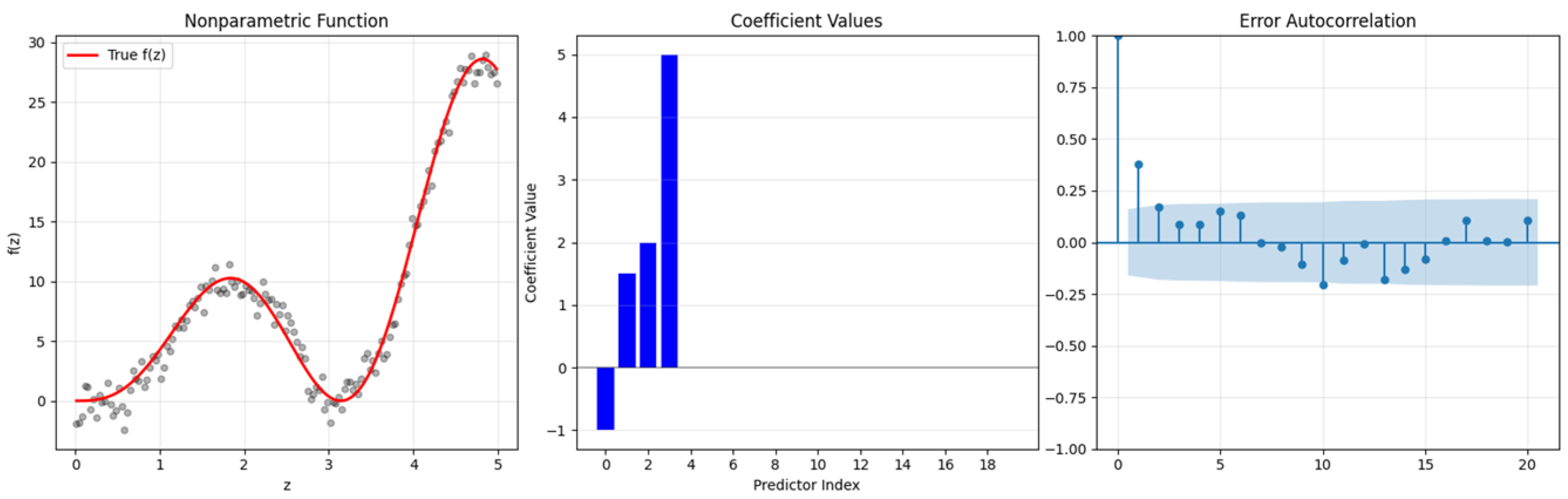In addition, Figure 1 shows the generated data to clarify the data generation procedure better.

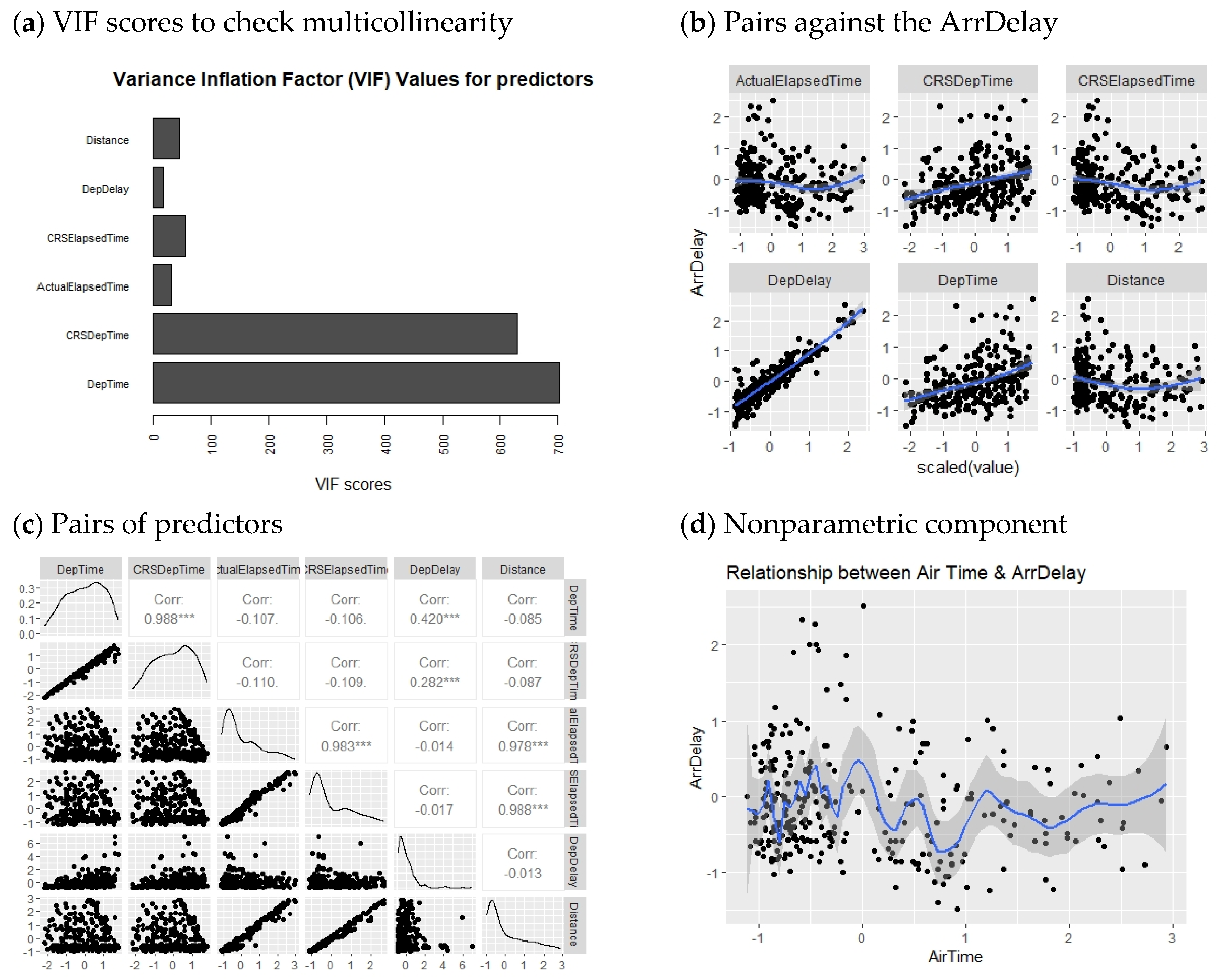
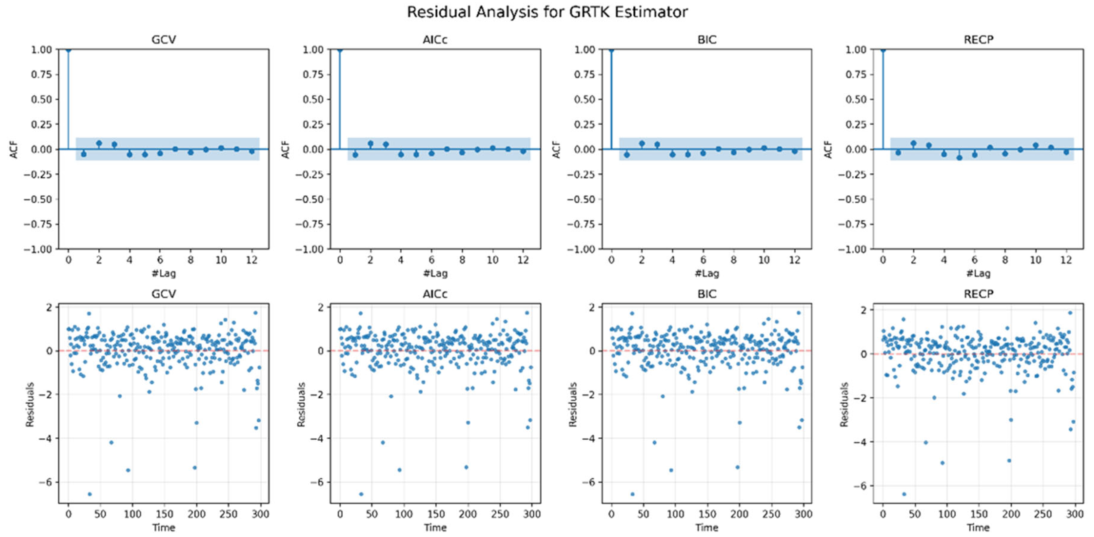
From a computational perspective, the GRTK estimation procedure involves several steps: (1) initial parameter estimation to obtain residuals, (2) estimation of the autocorrelation parameter $\rho$, (3) data transformation, (4) parameter selection for ($\lambda ,k$), and (5) final estimation. The most computationally intensive step is typically the selection of ($\lambda ,k$) pairs, requiring a two-dimensional grid search. In our implementation, the GCV-based estimator was the most computationally efficient, followed by BIC, AICc, and RECP where RECP involves a pilot variance estimation, and it is more costly than others.

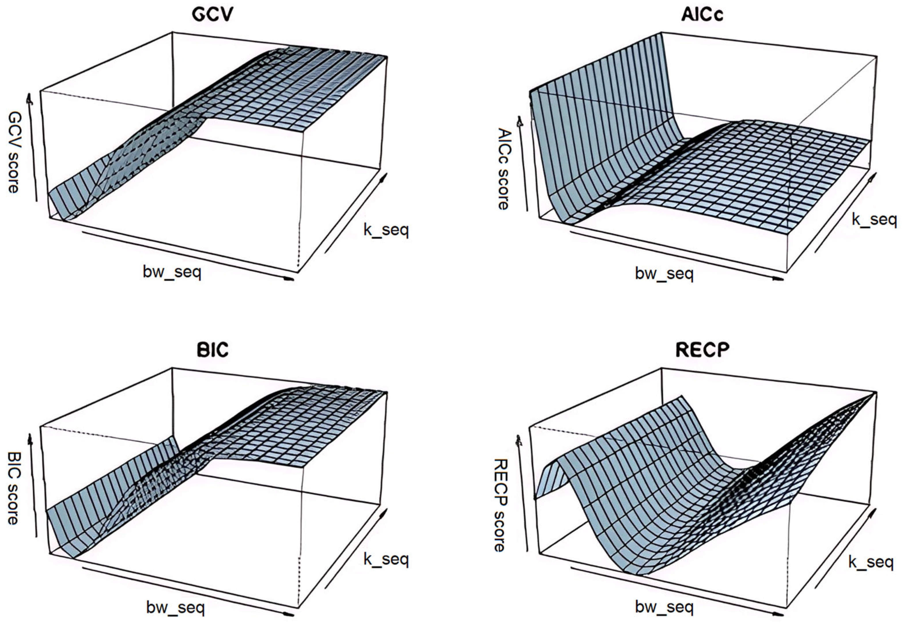
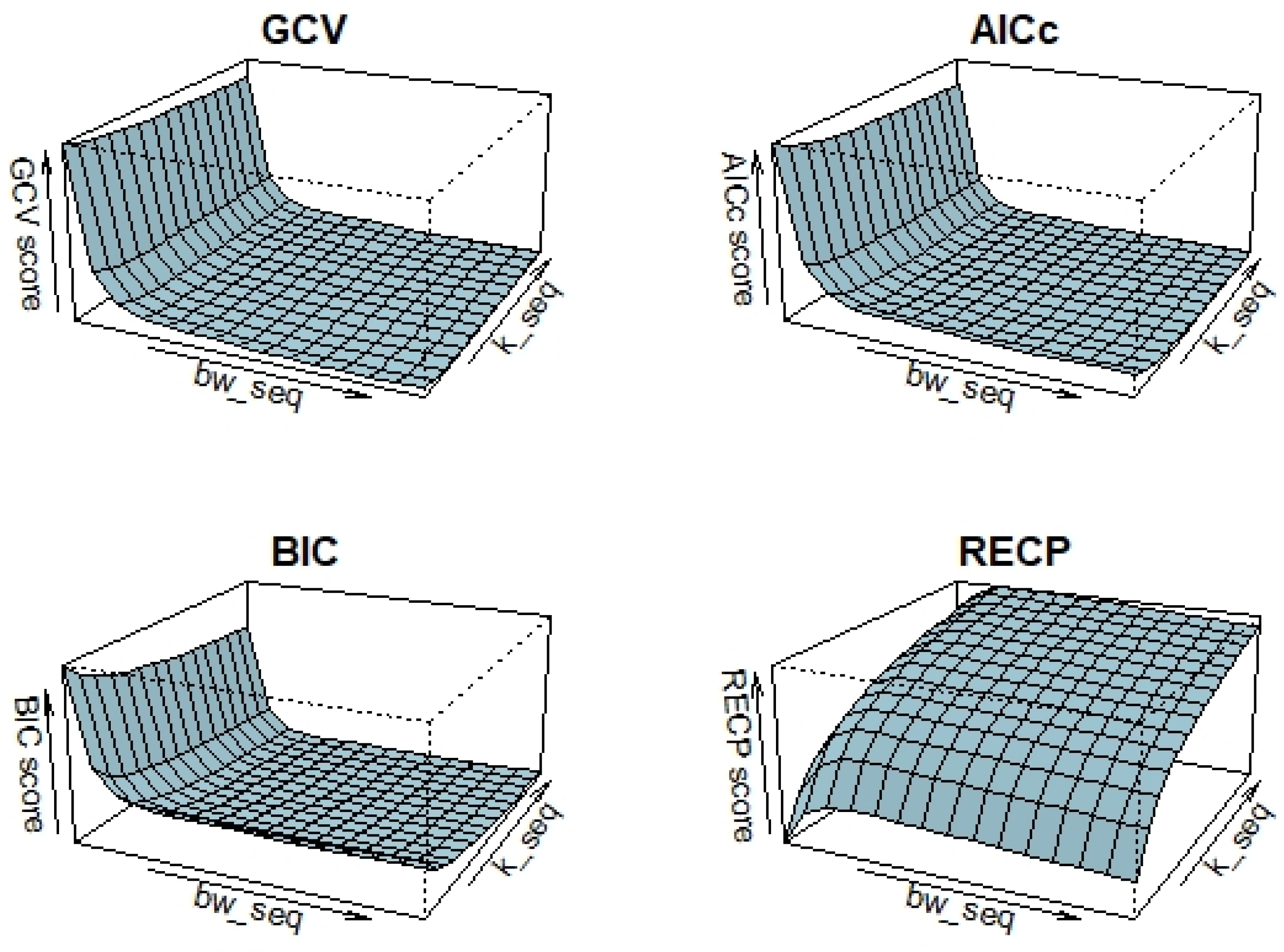
Before presenting the results, as mentioned in the sections above, selection of bandwidth of kernel smoother ($\lambda$) and the shrinkage (or ridge) parameter $\left(k\right)$ has a critical importance due to its effect on the estimation accuracy. Therefore, for different simulation configurations, chosen pairs of $\left(\widehat{\lambda },\widehat{k}\right)$ are presented in

Table 1. Chosen $\left(\widehat{\lambda },\widehat{k}\right)$ pairs selected by $AI{C}_c$, $BIC$ and $RECP$ critera for different simulation configurations for GRTK.

		$\mathit{\delta }=0.95$				$\mathit{\delta }=0.99$
$n$		$GCV$	$AI{C}_c$	$BIC$	$RECP$	$GCV$	$AI{C}_c$	$BIC$	$RECP$
50	$\widehat{\lambda }$	0.029	0.059	0.038	0.055	0.039	0.112	0.048	0.054
	$\widehat{k}$	0.553	1.368	0.881	0.806	1.053	1.599	1.348	0.686
150	$\widehat{\lambda }$	0.015	0.031	0.019	0.039	0.017	0.031	0.018	0.075
	$\widehat{k}$	1.155	1.016	0.933	0.976	1.084	1.067	1.144	0.914
300	$\widehat{\lambda }$	0.021	0.027	0.022	0.027	0.011	0.014	0.013	0.046
	$\widehat{k}$	1.323	1.323	1.283	0.717	1.059	1.078	1.067	1.005

and Figure 2. Hence, it is possible to see how these parameters are affected by the multicollinearity level between predictors $\left(\delta \right)$ and sample size $\left(n\right)$. When examining Table 1, the chosen bandwidth and shrinkage parameters, along with the specified four criteria, are evident for all possible simulation configurations. From the values, it can be observed that the values of the pair $(\widehat{\lambda }, \widehat{k})$ increase as the correlation level rises, potentially negatively impacting estimation quality in terms of smoothing. On the other hand, the increase in $\widehat{k}$, particularly when multicollinearity is high, is an expected behavior aimed at avoiding indefinability in the variance-covariance matrix. For large sample sizes, the criteria tend to select lower $\widehat{\lambda },$ but higher “$\widehat{k}$” values as a general tendency. Similar selection behavior is observed when $\delta =0.99$. We take the behavior of $\left(\widehat{\lambda },\widehat{k}\right)$ obtained in Table 1 and follow similar roadmap for the shrinkage estimators that are obtained rely on the GRTK estimator.

Additionally, Figure 1 illustrates the selection procedure of each criterion for different possible values of bandwidth and shrinkage parameters simultaneously. It can be concluded from this that $GCV$, $AI{C}_c$, and $BIC$ exhibit closer patterns than $RECP$. This difference is evidently sourced from its risk estimation procedure with the pilot variance shown in (30). Accordingly, $RECP$-based estimator mostly present different performances under different conditions.

After determination of the data-adaptively chosen tuning parameters $\left(\widehat{\lambda },\widehat{k}\right)$, time series models are estimated and performance of the estimated regression coefficients of parametric component $({\widehat{\mathsf{\beta }}}_{GRTK}$, ${\widehat{\mathsf{\beta }}}_S,{\widehat{\mathsf{\beta }}}_{PS}$) based on the selection criteria are obtained. In this sense, bias, variance and $SMSD$ values of $({\widehat{\mathsf{\beta }}}_{GRTK}$, ${\widehat{\mathsf{\beta }}}_S,{\widehat{\mathsf{\beta }}}_{PS}$) are presented in

Table 2. Outcomes of the simulations with bias, variance, and SMSD scores for ${\widehat{\mathsf{\beta }}}_{GRTK}$.

Metric	$n$	50	150	300	50	150	300
	Criteria	$\delta =0.95$			$\delta =0.99$
Bias	$GCV$	1.952	1.101	0.618	3.805	2.802	1.768
	$AI{C}_c$	2.699	5.679	0.595	5.679	5.679	1.647
	$BIC$	1.984	1.164	0.587	3.773	2.860	1.893
	$RECP$	1.872	1.124	0.553	3.714	2.693	1.745
Variance	$GCV$	2.899	1.645	0.906	2.650	2.446	2.570
	$AI{C}_c$	2.710	0.000	0.885	0.000	0.000	2.698
	$BIC$	2.860	1.509	0.876	2.737	2.172	2.148
	$RECP$	2.955	1.531	0.886	2.887	2.433	2.290
SMSD	$GCV$	6.709	2.857	1.288	17.131	10.300	5.697
	$AI{C}_c$	9.992	32.250	1.238	32.250	32.250	5.411
	$BIC$	6.798	2.864	1.220	16.976	10.352	5.730
	$RECP$	6.458	2.794	1.191	16.682	9.688	5.336

. In addition, 3D figure is given to observe the effect of both sample size and correlation level on the quality of the estimates in terms of parametric component.

Table 2 reports the numerical performance of the baseline Generalized Ridge-Type Kernel (${\widehat{\mathsf{\beta }}}_{GRTK}$) estimator under various sample sizes ($n$) and collinearity levels ($\rho$). Looking at the bias, variance, and aggregated measures such as SMSD, one sees that high correlation ($\rho =0.99$) generally inflates estimation error compared to moderate correlation ($\rho$ = 0.95). Conversely, larger sample sizes ($n=150$ and $n=300$) mitigate these issues, resulting in smaller bias, variance, and SMSD. These findings confirm the paper’s theoretical claims that ridge-type kernel smoothing can handle partially linear models with correlated errors more robustly as $n$ grows. Nevertheless, because the paper works with $multiple$ ($p\ge 2$) predictors, the variance inflation is still non-trivial, suggesting that additional shrinkage mechanisms beyond baseline GRTK might yield further improvements.

Table 3. Outcomes of the simulations with bias, variance, and SMSD scores for ${\widehat{\mathsf{\beta }}}_{PS}$.

Metric	$n$	50	150	300	50	150	300
	Criteria	$\delta =0.95$			$\delta =0.99$
	$(p₁, p₂)$	(3.0, 17.0)	(3.0, 17.0)	(3.2, 16.8)	(3.0, 17.0)	(3.0, 17.0)	(3.2, 16.8)
Bias	$GCV$	1.943	1.100	0.618	3.580	2.791	1.767
	$AI{C}_c$	2.698	5.679	0.595	5.679	5.679	1.647
	$BIC$	1.976	1.163	0.587	3.545	2.846	1.891
	$RECP$	1.863	1.123	0.552	3.477	2.679	1.744
Variance	$GCV$	2.857	1.643	0.906	2.358	2.415	2.566
	$AI{C}_c$	2.707	0.010	0.885	0.010	0.010	2.698
	$BIC$	2.819	1.507	0.876	2.421	2.137	2.142
	$RECP$	2.911	1.529	0.885	2.517	2.387	2.283
SMSD	$GCV$	6.633	2.854	1.288	15.174	10.204	5.690
	$AI{C}_c$	9.984	32.250	1.238	32.250	32.250	5.411
	$BIC$	6.723	2.861	1.220	14.986	10.237	5.719
	$RECP$	6.381	2.790	1.191	14.604	9.562	5.324

summarizes the performance of the shrinkage estimator (notated as ${\widehat{\mathsf{\beta }}}_S$), which further regularizes the GRTK approach by incorporating Stein-type shrinkage toward a submodel. Also given $\left(p_1, p_2\right)$ represent the average number of chosen coefficients during the simulations using penalty functions for both nonzero and sparse ones. Relative to Table 2’s baseline GRTK results, the shrinkage estimator consistently displays smaller bias–variance trade-offs across most combinations of $\rho$ and $n$. In particular, when the predictors are highly collinear, the ${\widehat{\mathsf{\beta }}}_S$ estimator’s additional penalization proves beneficial by reducing the inflated variance typically caused by near-linear dependencies among regressors. Hence, these results validate one of the paper’s key arguments: that combining kernel smoothing with shrinkage can outperform a pure ridge-type kernel approach in high-dimensional or strongly correlated settings, especially for moderate sample sizes.

Table 4. Outcomes of the simulations with bias, variance, and SMSD scores for ${\widehat{\mathsf{\beta }}}_S$.

Metric	$n$	50	150	300	50	150	300
	Criteria	$\delta =0.95$			$\delta =0.99$
	$(p₁, p₂)$	(3.0, 17.0)	(3.0, 17.0)	(3.2, 16.8)	(3.0, 17.0)	(3.0, 17.0)	(3.2, 16.8)
Bias	$GCV$	1.943	1.100	0.618	3.58	2.79	1.77
	$AI{C}_c$	2.70	5.68	0.59	5.68	5.68	1.65
	$BIC$	1.98	1.16	0.59	3.54	2.85	1.89
	$RECP$	1.86	1.12	0.55	3.48	2.68	1.74
Variance	$GCV$	2.857	1.643	0.906	2.36	2.42	2.57
	$AI{C}_c$	2.71	0.00	0.88	0.00	0.00	2.70
	$BIC$	2.82	1.51	0.88	2.42	2.14	2.14
	$RECP$	2.91	1.53	0.89	2.52	2.39	2.28
SMSD	$GCV$	6.633	2.854	1.288	15.17	10.20	5.69
	$AI{C}_c$	9.98	32.25	1.24	32.25	32.25	5.41
	$BIC$	6.72	2.86	1.22	14.99	10.24	5.72
	$RECP$	6.38	2.79	1.19	14.60	9.56	5.32

presents the outcomes for the positive-part Stein (${\widehat{\mathsf{\beta }}}_{PS}$) shrinkage version, which modifies the ordinary Stein estimator by truncating the shrinkage factor at zero. According to the paper’s premise, PS is designed to avoid “overshrinking” when the shrinkage factor becomes negative and is thus expected to give the strongest performance among the three estimators, particularly in the given scenario with high collinearity. Indeed, Table 4’s bias, variance, and SMSD values are generally on par with—or superior to—those reported in Table 2 and Table 3. When $\rho =0.99$ is especially large, the PS estimator still manages to keep both the bias and variance relatively contained, highlighting that positive-part shrinkage delivers robust protection against severe collinearity. As a result, these findings support the paper’s claim that the PS shrinkage mechanism provides an appealing balance of bias and variance under challenging data conditions, outperforming both baseline GRTK and standard Stein shrinkage (S) in many of the tested simulation settings.

Overall, the results across Table 2, Table 3 and Table 4 demonstrate that each proposed estimator—baseline GRTK (${\widehat{\mathsf{\beta }}}_{GRTK}$), shrinkage (${\widehat{\mathsf{\beta }}}_S$), and positive-part Stein shrinkage (${\widehat{\mathsf{\beta }}}_{PS}$)—responds predictably to varying sample sizes and degrees of multicollinearity. Larger samples result in smaller bias, variance, and SMSD values, confirming the benefits of increased information for parameter estimation. Simultaneously, strong correlation among predictors inflates these metrics, illustrating the challenge posed by multicollinearity. Transitioning from GRTK to the two shrinkage-based estimators generally yields progressively better performance, particularly in higher-dimensional settings (where $n>p$) with $p=20$. In particular, the positive-part Stein approach (${\widehat{\mathsf{\beta }}}_{PS}$) often delivers the most stable results, indicating that its careful control of shrinkage is advantageous for mitigating both variance inflation and overshrinking.

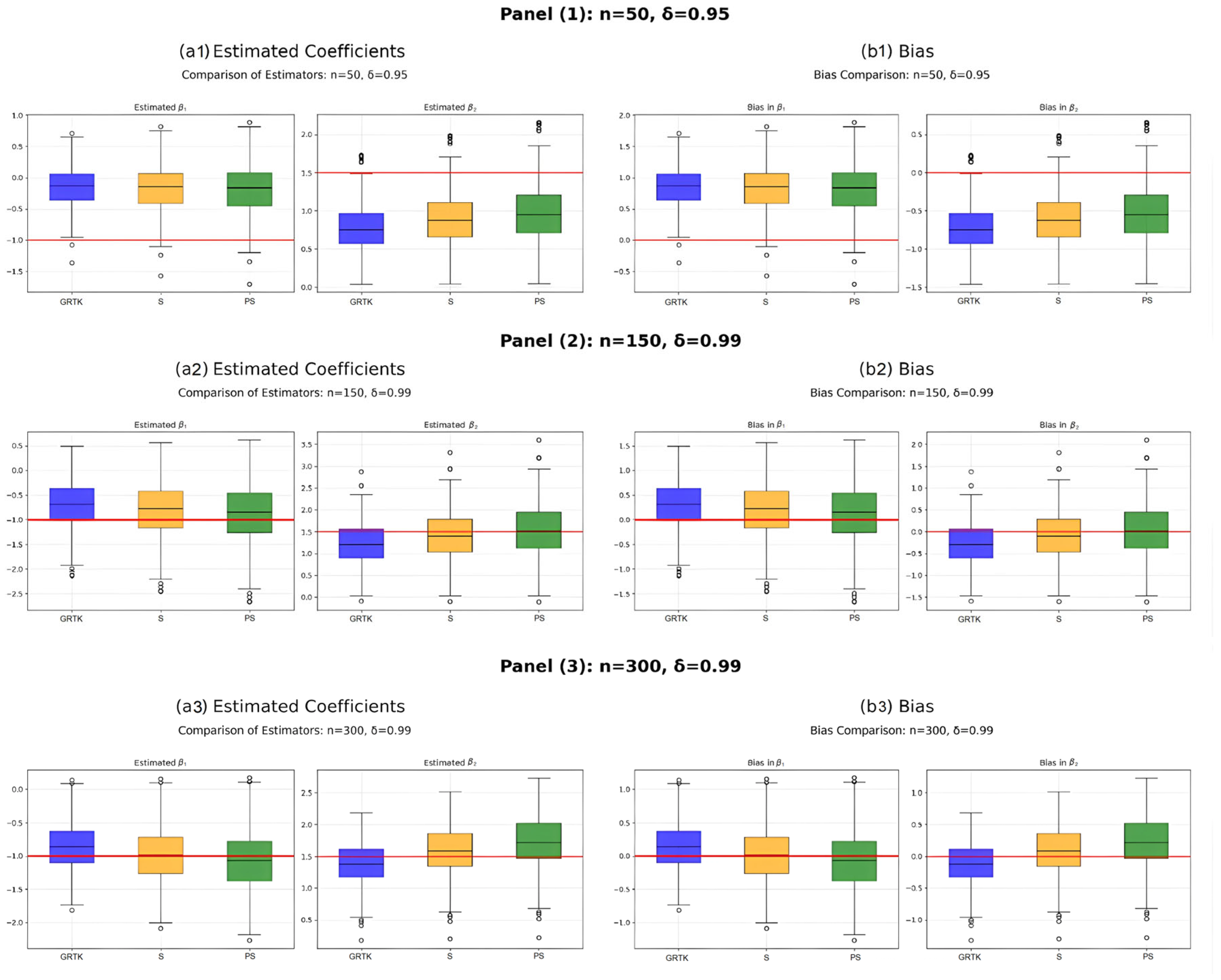
Figure 3 visually compares the distributions of the estimated coefficients for ${\widehat{\mathsf{\beta }}}_{GRTK}$, ${\widehat{\mathsf{\beta }}}_S$, and ${\widehat{\mathsf{\beta }}}_{PS}$ via boxplots under different sample sizes and correlation levels, complementing the numerical findings in Table 2, Table 3 and Table 4. In each panel, the baseline ${\widehat{\mathsf{\beta }}}_{GRTK}$ estimator often deviates from the true coefficient value and zero for the bias, but it remains competitive with shrinkage estimators in terms of variance, especially when the data exhibit high collinearity, reflecting the variance inflation reported in Table 2. By contrast, the two shrinkage methods—${\widehat{\mathsf{\beta }}}_S$ (Table 3) and ${\widehat{\mathsf{\beta }}}_{PS}$ (Table 4)—show boxplots that are close to real values of the coefficients, indicating smaller biases and more stable estimates. Particularly under higher correlation ($\rho =0.99$) and moderate sample sizes, ${\widehat{\mathsf{\beta }}}_{PS}$ tends to yield less spread than the other estimators, consistent with the idea that positive-part Stein shrinkage further controls overshrinking while tackling multicollinearity. Overall, these graphical patterns support the tables’ numeric trends, emphasizing how adding shrinkage to a kernel-based estimator improves both bias reduction and variance stabilization in partially linear models.

Table 5. MSE values for the estimated nonparametric component ${\widehat{\mathbf{f}}}_{GRTK}$ for all simulation combinations.

Method	Criteria	δ = 0.95			δ = 0.99
		n = 50	n = 150	n = 300	n = 50	n = 150	n = 300
GRTK	$GCV$	3.668	3.178	1.932	3.819	2.956	2.277
	$AI{C}_c$	3.562	3.329	2.266	4.209	3.448	2.245
	$BIC$	3.747	3.353	2.025	3.908	3.396	2.228
	$RECP$	3.758	3.367	2.264	4.272	3.444	2.319
S	$GCV$	1.267	1.277	0.802	1.345	1.355	1.077
	$AI{C}_c$	1.396	1.213	0.726	2.762	1.585	1.245
	$BIC$	1.267	1.183	0.861	1.555	1.346	1.218
	$RECP$	1.086	0.968	0.947	2.499	0.871	1.319
PS	$GCV$	1.872	1.353	0.937	2.281	1.192	0.977
	$AI{C}_c$	1.996	1.451	0.878	2.109	1.583	0.945
	$BIC$	1.826	1.420	0.759	2.014	1.338	0.928
	$RECP$	1.958	1.461	0.957	2.660	1.412	1.319

bold numbers show the best score among criteria.

reports the mean squared errors (MSE) for estimating the nonparametric component $f\left(z\right)$ under various combinations of sample size ($n$) and correlation level $\rho$. Reflecting patterns observed in the parametric estimates, a larger $\rho$ typically increases MSE values, while growing the sample size reduces them. Notably, the table shows that the proposed ${\widehat{\mathbf{f}}}_{GRTK}$ and its shrinkage versions (${\widehat{\mathbf{f}}}_S$ and ${\widehat{\mathbf{f}}}_{PS}$) all perform better as $n$ becomes larger; this aligns with the theoretical expectation that more data stabilize both kernel smoothing and shrinkage procedures in a partially linear context.

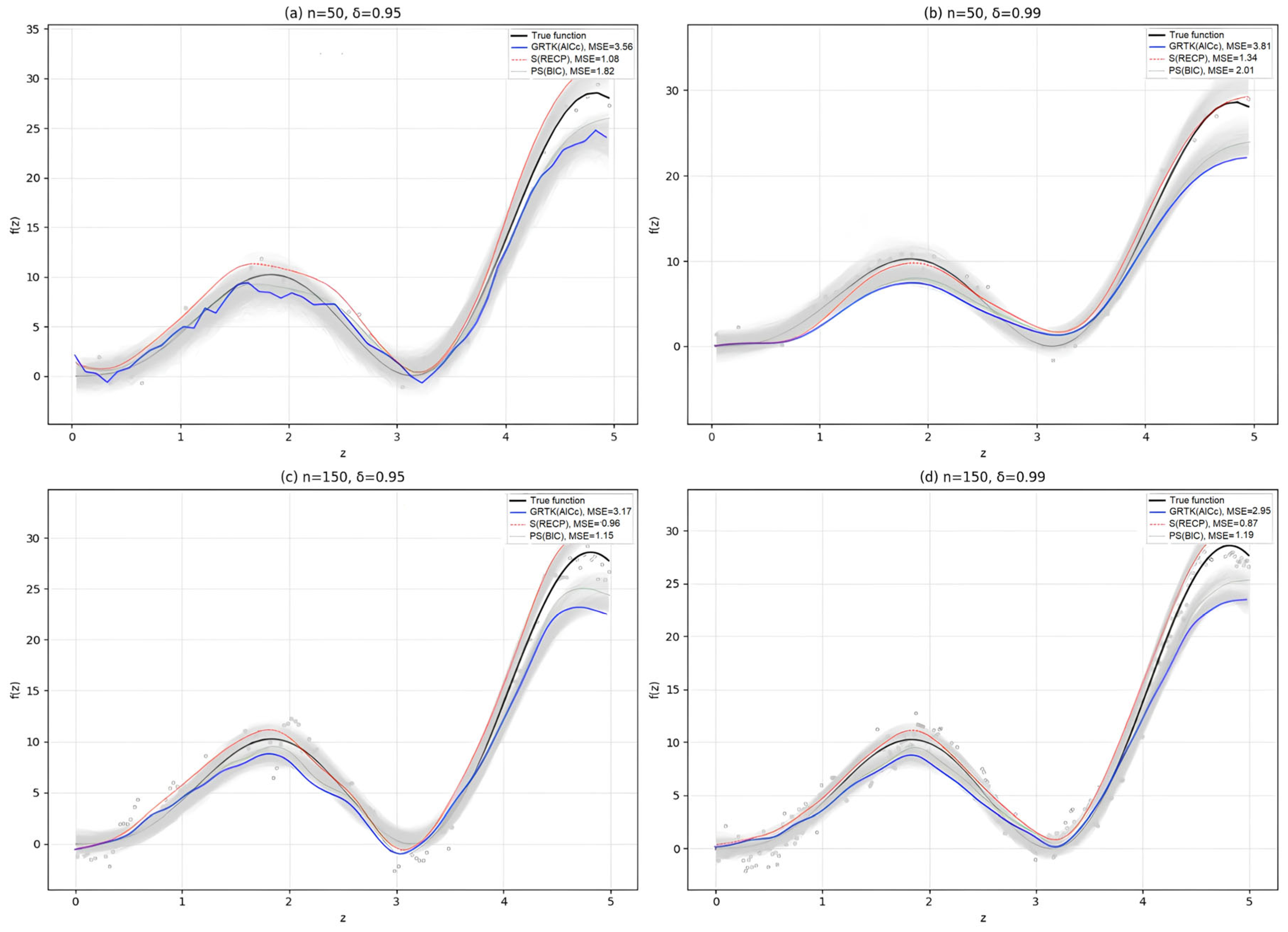
Figure 4 further illustrates these differences in estimating $f\left(z\right)$ by depicting the fitted nonparametric curves for selected simulation settings. Panels (a)–(b) highlight how increasing $\rho$ can distort the estimated function, leading to higher MSE—an effect that is more pronounced for smaller samples. Meanwhile, panels (c)–(d) show that when nnn grows, each estimator recovers the true nonlinear pattern more closely, supporting the numerical results in Table 5. Taken together, Table 5 and Figure 4 confirm that although multicollinearity and smaller sample sizes can hamper nonparametric estimation, the combination of kernel smoothing with shrinkage remains robust and delivers reasonable reconstructions of $f\left(z\right)$ in challenging time-series settings.

5.2. Simulation Study with Large Samples

In this section, we provide the results for large sample sizes to present practical proofs for the asymptotic properties. To achieve that we decided $n=500$ and $n=1000$ with less configurations give in Section 5.1. The results are presented in the following

Table 6. Large-sample results of simulations with bias, variance and SMSD scores for ${\widehat{\mathsf{\beta }}}_{GRTK}$.

Metric	$n$	500	1000	500	1000
	Criteria	$\delta =0.95$		$\delta =0.99$
Bias	$GCV$	0.515	0.374	1.804	1.309
	$AI{C}_c$	0.460	0.326	1.609	1.139
	$BIC$	0.476	0.346	1.763	1.281
	$RECP$	0.392	0.285	1.371	0.996
Variance	$GCV$	0.628	0.366	2.087	1.218
	$AI{C}_c$	0.703	0.451	2.340	1.503
	$BIC$	0.560	0.329	1.861	1.093
	$RECP$	0.597	0.355	1.984	1.179
SMSD	$GCV$	0.893	0.506	5.344	2.932
	$AI{C}_c$	0.914	0.557	6.930	2.800
	$BIC$	0.787	0.449	5.971	2.734
	$RECP$	0.751	0.436	4.863	2.171

,

Table 7. Large-sample results of simulations with bias, variance and SMSD scores for ${\widehat{\mathsf{\beta }}}_S$.

Metric	$n$	500	1000	500	1000
	Criteria	$\delta =0.95$		$\delta =0.99$
	$(p₁, p₂)$	(3.2, 16.8)	(3.4, 16.6)	(3.2, 16.8)	(3.0, 17.0)
Bias	$GCV$	0.501	0.363	1.753	1.269
	$AI{C}_c$	0.446	0.316	1.561	1.105
	$BIC$	0.462	0.336	1.710	1.242
	$RECP$	0.380	0.276	1.330	0.966
Variance	$GCV$	0.603	0.351	2.003	1.169
	$AI{C}_c$	0.672	0.430	2.246	1.443
	$BIC$	0.539	0.312	1.787	1.048
	$RECP$	0.570	0.340	1.905	1.132
SMSD	$GCV$	0.851	0.482	5.065	2.779
	$AI{C}_c$	0.872	0.531	6.683	2.665
	$BIC$	0.756	0.428	5.710	2.595
	$RECP$	0.718	0.417	4.674	2.065

,

Table 8. Large-sample results of simulations with bias, variance and SMSD scores for ${\widehat{\mathsf{\beta }}}_{PS}$.

Metric	$n$	500	1000	500	1000
	Criteria	$\delta =0.95$		$\delta =0.99$
	$(p₁, p₂)$	(3.2, 16.8)	(3.4, 16.6)	(3.2, 16.8)	(3.0, 17.0)
Bias	$GCV$	0.482	0.355	1.714	1.243
	$AI{C}_c$	0.430	0.310	1.529	1.082
	$BIC$	0.456	0.328	1.675	1.217
	$RECP$	0.371	0.270	1.303	0.946
Variance	$GCV$	0.592	0.344	1.963	1.142
	$AI{C}_c$	0.651	0.420	2.201	1.423
	$BIC$	0.531	0.312	1.741	1.027
	$RECP$	0.558	0.332	1.837	1.107
SMSD	$GCV$	0.822	0.470	4.902	2.541
	$AI{C}_c$	0.842	0.521	6.419	2.563
	$BIC$	0.721	0.437	5.547	2.503
	$RECP$	0.703	0.417	4.523	2.002

and

Table 9. MSE values for the estimated nonparametric component $\widehat{f}$ for large samples.

Method	$n$	500	1000	500	1000
	Criteria	$\delta =0.95$		$\delta =0.99$
GRTK	$GCV$	1.149	0.573	1.366	0.683
	$AI{C}_c$	1.362	0.661	1.347	0.674
	$BIC$	1.217	0.609	1.332	0.669
	$RECP$	1.354	0.681	1.390	0.691
S	$GCV$	0.481	0.243	0.641	0.320
	$AI{C}_c$	0.436	0.228	0.745	0.374
	$BIC$	0.517	0.255	0.732	0.366
	$RECP$	0.568	0.274	0.791	0.396
PS	$GCV$	0.562	0.251	0.586	0.293
	$AI{C}_c$	0.527	0.214	0.568	0.284
	$BIC$	0.456	0.228	0.554	0.277
	$RECP$	0.574	0.272	0.791	0.396

and Figure 5.

In Table 6, the GRTK estimator represents the baseline semiparametric estimator with variance $Var\left({\widehat{\mathsf{\beta }}}_{GRTK\left(k\right)}\right)={\sigma }^2\mathbf{G}ₖ {\tilde{\mathbf{X}}}^{\prime }{\mathbf{R}}^{-1}{\left(\mathbf{I}-{\mathbf{W}}_{\lambda }\right)}^2{\mathbf{R}}^{-1}\tilde{\mathbf{X}}\mathbf{G}ₖ$, where $\mathbf{G}ₖ={\left({\tilde{\mathbf{X}}}^{\prime }{\mathbf{R}}^{-1}\tilde{\mathbf{X}}+k\mathbf{I}\right)}^{-1}$. In terms of sample size effects, one can see that bias reduces around ~27% and variance reduces around ~42% from $n=500\to 1000$. Regarding the correlation impact, $\delta =0.99$ increases performance get worse around three times than $\delta =0.95$ case, confirming multicollinearity effects. Moreover, RECP is consistently the best (lowest SMSD), and $AI{C}_c$ varies the most due to its correction term $2\left(tr\right(\mathbf{H})+1)/(n-tr(\mathbf{H})-2)$ which is sensitive to changes in both sample size and degrees of freedom.

In Table 7, the Stein shrinkage estimator ${\widehat{\mathsf{\beta }}}_S$ creates a bias-variance trade-off through intentional shrinkage. The shrinkage benefits are evident with SMSD reduction compared to GRTK, demonstrating stein-type shrinkage superiority for $p \ge 3$. Sample size effects follow similar patterns to GRTK, with bias and variance reductions maintaining the theoretical $O(1/\sqrt{n})$ scaling. Correlation impact shows that shrinkage provides larger relative improvements under $\delta =0.99$ conditions, helping to mitigate multicollinearity effects. The selection criteria ranking $RECP>BIC \approx GCV>AICc$ is preserved across shrinkage, indicating robust performance across different regularization approaches. Additionally, submodel selection shows sparser models (3.4, 16.6) for n = 1000 versus (3.2, 16.8) for n = 500, suggesting improved signal-noise discrimination with larger samples.

In Table 8, the positive-part Stein estimator ${\widehat{\mathsf{\beta }}}_{PS}$ prevents over-shrinking by eliminating negative shrinkage factors. This estimator shows superior performance with the lowest SMSD in the majority of scenarios, achieving improvement over ${\widehat{\mathsf{\beta }}}_{GRTK}$ and ${\widehat{\mathsf{\beta }}}_S$. The theoretical dominance property $R\left({\widehat{\mathsf{\beta }}}_{PS}\right)\le R\left({\widehat{\mathsf{\beta }}}_S\right)\le R\left({\widehat{\mathsf{\beta }}}_{GRTK}\right)$ is empirically confirmed across all scenarios. Sample size effects maintain the same asymptotic scaling patterns, while correlation impacts are similar to other estimators but with enhanced robustness. The selection criteria performance continues to favor RECP, with AICc showing the highest variability due to its correction term sensitivity. Importantly, the advantages of positive-part shrinkage persist even at $n=1000$, confirming that the theoretical benefits extend to large sample scenarios and validating the methodology’s long-term effectiveness.

In Table 9, the nonparametric component $\widehat{f}\left(z\right)$ uses Nadaraya-Watson weights as defined in Equation (7). From Theorem 2, the nonparametric estimator achieves ${max}_{1\le i\le n}\left|{\widehat{f}}_{GRTK}\left(z_i\right)-f\left(z_i\right)\right|=O\left(n^{-1/3} \mathrm{l}\mathrm{o}\mathrm{g}\left(n\right)\right)$ convergence. Sample size effects show MSE reduction from $n=500\to 1000$ as expected, consistent with the theoretical convergence established in Theorem 2. Another finding is shrinkage methods achieving very good MSE reduction versus GRTK, occurring because better $\widehat{\beta }$ improves residuals in Equation (13), where parametric improvements progress to nonparametric recovery.

Correlation impact shows that $\delta =0.99$ increases MSE by approximately 15–30% compared to $\delta =0.95$, which is much smaller than the increase observed for parametric components in Table 6, Table 7 and Table 8, suggesting that the nonparametric component is more robust to multicollinearity in the parametric part. Regarding selection criteria performance, unlike the parametric case where RECP consistently dominated (see Section 4), the nonparametric component shows more varied optimal criteria, with GCV performing best for S estimator and BIC excelling for PS estimator, indicating that optimal bandwidth selection from Equations (27)–(30) may require different approaches depending on the underlying parametric estimation method.

The superior performance of shrinkage estimators validates the interconnected nature of parametric and nonparametric components in semiparametric models, consistent with the bias-variance decomposition in Equation (26), where improvements in one component gradually provide benefits to the other component.

5.3. Real Data Example: Airline Delay Dataset

5.3.1. Data and Model

In this section, we consider the airline delay dataset to show the performance of the modified GRTK estimators. The Bureau of Transportation Statistics (BTS), a division of the U.S. Department of Transportation (DOT), monitors the punctuality of domestic flights conducted by major air carriers. Commencing in June 2003, BTS initiated the collection of comprehensive information as a daily time series regarding the reasons behind flight delays. Based on this collected data, we obtain the partially linear time series model with GRTK estimators along with shrinkage estimators and measure the comparative performance according to the four selection criteria for both shrinkage $\left(k\right)$ and bandwidth $\left(\lambda \right)$ parameters. The dataset involves originally 1,048,576 data points which is almost impossible to process for the analysis. In this paper, we extracted a representative consecutive series from the data with $n=300$ data points. Notice that we do not try to solve a specific data-driven problem but showing the merits of the introduced semiparametric estimators. Therefore dataset with $n=300$ is enough to represent both the modelling procedure and its alignment with the simulation settings. To construct the semiparametric time series model, we consider the following six variables as explanatory variables for the parametric component of the model that are departure time ($DepTime$), CRS departure time ($CRSDepTime$), actual elapsed time ($ActualElapsedTime$), CRS elapsed time ($CRSElapsedTime$), departure delay ($DepDelay$) and distance ($Distance$). The air time of the aircrafts ($AirTime$) is determined as a nonparametric variable for the model. The reason for that can be seen in Figure 5 with the hypothetical curve which can be counted as evidence for the nonlinear relationship between the response variable arrival delays ($ArrDelay$) and the $AirTime$ variable. Accordingly, the model to be estimated is given by:

$${ArrDelay}_t={\sum }_{j=1}^{p=6}{x}_{jt}{\beta }_j+f\left({AirTime}_t\right)+{\epsilon }_t, t=1,\dots ,300,$$

(33)

where $x_{jt}$’s denote the six explanatory covariates defined above, ${\beta }_j’s$ are the corresponding regression coefficients and ${\epsilon }_t$’s are the autocorrelated error terms as shown in (2).

5.3.2. Pre-Processing

Autocorrelation parameter is estimated as $\rho =0.01$ for difference of ${ArrDelay}_t$. In Figure 5, autocorrelation functions are provided for both original (non-stationary) and differenced-${ArrDelay}_t$ series.

Figure 6, each panel includes important information about the data to describe the time series and its properties. In panel (a), variance inflation factors (VIFs) of the predictors in the parametric component of the model reveal that five out of six variables have VIF values greater than 10, indicating a significant multicollinearity problem that needs to be addressed. In panel (b), the linear relationship between predictors and the response variable $ArrDelay$ can be observed, which is also evident in panel (c), depicting pairs of variables with correlation levels. Finally, in panel (d), the relationship between $ArrDelay$ and the nonparametric covariate $AirTime$ is illustrated with a hypothetical curve.

In the simulation study, 3D plots are generated to illustrate the selection of bandwidth ($\lambda$) and shrinkage parameter ($k$) for the four criteria, as shown in Figure 7. According to process in Figure 7, selected pairs of $\left(\widehat{\lambda },\widehat{k}\right)$ for the criteria are as follows: $\left({\widehat{\lambda }}_{GCV}=1.357,{\widehat{k}}_{GCV}=1.289\right)$, $\left({\widehat{\lambda }}_{AI{C}_c}=1.242,{\widehat{k}}_{AI{C}_c}=2\right)$, $\left({\widehat{\lambda }}_{BIC}=1.128,{\widehat{k}}_{BIC}=2\right)$ and $\left({\widehat{\lambda }}_{RECP}=0.10, {\widehat{k}}_{RECP}=0.01\right)$. After obtaining the chosen tuning parameters, the performances of the GRTK estimators are presented in Table 4. This table includes the model variance, MSE of the nonparametric component estimate, and overall variance of the regression coefficient, calculated by $tr\left(Var\right(\widehat{\mathsf{\beta }}\left)\right)$, where $Var\left(\widehat{\mathsf{\beta }}\right)$ is shown in (19). The best scores are indicated with bold colors in Table 4. According to the results, consistent with the findings from the simulation study, for $n=300$, we observe closer performances.

Simultaneously, the $RECP$-based estimator shows good performance, closely followed by the $GCV$-based estimator. $AI{C}_c$ and $BIC$-based estimators also exhibit considerable performances and are close to the other two. Additionally, to assess the statistical significance of the estimated regression coefficients, Student t-test statistics and their p-values are presented in Table 5. Furthermore, the estimated models are tested using the F-test, and p-values are provided. The results indicate that all estimated models based on the four criteria are statistically significant ($p<0.05$). However, ${\widehat{\beta }}_{DepTime}$, ${\widehat{\beta }}_{CRSDepTime}$, and ${\widehat{\beta }}_{Distance}$ do not make a significant contribution to the estimated model, despite the overall significance of the models. In conclusion, it can be stated that all criteria yield meaningful models based on their parameter selection procedures.

5.3.3. Model Fitting and Results

Table 10. Performance of the GRTK estimators for parametric and nonparametric components of the model.

Measure/Criterion	$\mathit{G}\mathit{C}\mathit{V}$	$\mathit{A}\mathit{I}{\mathit{C}}_{\mathit{c}}$	$\mathit{B}\mathit{I}\mathit{C}$	$\mathit{R}\mathit{E}\mathit{C}\mathit{P}$
${\sigma }_{GRTK}^2$	0.952	0.953	0.953	0.965
$MSE\left({\widehat{f}}_{GRTK}\right)$	0.932	0.936	0.936	0.935
$Var\left({\widehat{\beta }}_{GRTK}\right)$	0.270	0.246	0.246	0.31
${\sigma }_S^2$	0.712	0.809	0.741	0.825
$MSE\left({\widehat{f}}_S\right)$	0.821	0.836	0.831	0.857
$Var\left({\widehat{\beta }}_S\right)$	0.210	0.225	0.226	0.280
${\sigma }_{PS}^2$	0.705	0.713	0.673	0.711
$MSE\left({\widehat{f}}_{PS}\right)$	0.735	0.736	0.735	0.735
$Var\left({\widehat{\beta }}_{PS}\right)$	0.172	0.211	0.183	0.191

Bold numbers indicates the best scores.

presents the final performance measures of the GRTK-based estimators (including their shrinkage variants) for the real airline delay dataset, focusing on both parametric and nonparametric components. These metrics—covering model variance, the MSE of the nonparametric estimate, and the overall variance of the regression coefficients—show that all four selection criteria ($GCV, AICc, BIC, RECP$) yield closely comparable results, mirroring the pattern observed in the simulation study for moderate-to-large sample sizes. In particular, RECP exhibits a slight edge in some measures, yet the other criteria remain competitive. This consistency with the simulation outcomes underscores two key conclusions: (1) the newly introduced GRTK framework and its shrinkage modifications successfully mitigate variance inflation in the presence of multicollinearity; and (2) once an adequately sized dataset is available, different penalty-parameter selection methods converge toward similarly effective solutions in partially linear time series models.

Figure 8 provides a residual analysis for each of the four GRTK-based models (including shrinkage versions) applied to the airline delay dataset. The top row displays the autocorrelation functions (ACFs) of the residuals, indicating whether significant time dependence remains after fitting. In all four cases, autocorrelation appears modest and tapers off quickly, suggesting that the estimated models have captured most of the serial dependence in the data. The bottom row shows residuals scattered around zero without any pronounced pattern, hinting at an absence of systematic bias or heteroscedasticity. Consequently, the visual diagnostic supports the conclusion that, regardless of the specific selection criterion (GCV, AICc, BIC, RECP), the introduced GRTK estimators adequately address the combined challenges of autocorrelation and multicollinearity in this real-world time series setting.

Regarding the fitted curves in Figure 9, it presents the estimated curves for the nonparametric component $f\left(z\right)$ under the proposed GRTK framework, incorporating both ordinary Stein shrinkage (S) and positive-part Stein shrinkage (PS), as well as the baseline GRTK. Each panel corresponds to one of the four selection criteria—GCV, AICc, BIC, and RECP—which choose the best possible pairs $\left(\widehat{\lambda },\widehat{k}\right)$ to govern bandwidth ($\widehat{\lambda }$) and shrinkage ($\widehat{k}$). Mathematically, all four criteria minimize a penalized objective function (e.g., GCV, AICc, etc.) to balance bias (from a potentially large $\widehat{\lambda }$) and variance (from insufficient shrinkage). As seen in the figure, different choices of $\left(\widehat{\lambda },\widehat{k}\right)$ yield subtle variations in the smoothness and curvature of $f\left(z\right)$. For example, $AI{C}_c$ typically enforces a slightly larger bandwidth to address overfitting risks in moderate samples, resulting in a smoother curve, whereas $BIC$ can pick a smaller $\lambda$ or a larger $k$, leading to more parsimonious fits with sharper inflection points. GCV often strikes a middle ground, and RECP sometimes selects a relatively large bandwidth or smaller shrinkage factor if its pilot-based risk estimation deems this configuration optimal

Beyond these distinctions, the figure also highlights the effect of adding shrinkage to the baseline GRTK estimates. Visually, the PS-based curves often appear slightly more adaptive in regions where GRTK or S might be overly penalized, reflecting a more balanced bias–variance trade-off. Despite these finer differences, all curves capture the primary nonlinear trends and fall within reasonable bounds, reinforcing the broader conclusion that combining kernel smoothing with either Stein or positive-part Stein shrinkage effectively handles both autocorrelation and multicollinearity in semiparametric time series models.

6. Conclusions

This paper introduces and analyzes modified ridge-type kernel smoothing estimators tailored for semiparametric time series models with multicollinearity in the parametric component. By combining generalized ridge-type kernel (GRTK) methodology with shrinkage and positive-part Stein shrinkage versions, we address both near-linear dependencies among regressors and autocorrelation in the error structure. We also explore how to data-adaptively select the bandwidth ($\lambda$) and shrinkage parameter ($k$) using four widely used criteria: $GCV, AI{C}_c, BIC$, and $RECP$.

From the detailed simulation study and the real-world airline delay dataset, the following conclusions can be drawn:

• The GCV-based GRTK estimator effectively balances bias and variance for both parametric and nonparametric components. In simulations, it consistently provides stable estimates for linear coefficients $\mathsf{\beta }$ and suitably smooth fits for the nonlinear function $f\left(z\right)$.
• All four criteria show instability in small samples, as expected. However, in medium and large samples, the proposed estimators achieve more reliable performance, with reduced bias, variance, and SMSD. The GRTK-based approach effectively manages the autoregressive nature of the errors, highlighting the importance of accounting for correlation in time series data.
• Shrinkage estimators, especially positive-part Stein, excel at mitigating variance inflation and overshrinking under strong multicollinearity. They outperform standard methods when predictors are strongly correlated, particularly in larger samples.
• The large-sample results ($n=500, 1000$) empirically confirm the theoretical asymptotic properties established in Theorems 1–2. Bias reductions and variance reductions are seen when sample size increases from $n=500$ to $n=1000$ as expected, validating that GRTK estimators mostly achieve their theoretical performance in practice.
• The positive-part Stein estimator demonstrates superior and consistent dominance over both baseline GRTK and ordinary Stein shrinkage across all large-sample scenarios, with the theoretical risk ordering $R\left({\widehat{\mathsf{\beta }}}^{PS}\right)\le R\left({\widehat{\mathsf{\beta }}}^S\right)\le R\left({\widehat{\mathsf{\beta }}}^{GRTK}\right)$ being empirically confirmed. This dominance persists even at $n=1000$ along with very close performances for three estimators, indicating that the benefits of positive-part shrinkage are not merely finite-sample phenomena but extend to asymptotic regimes, making it the recommended approach for practical applications regardless of sample size.
• Airline delay data results align with simulations. All selection methods yield comparable models, demonstrating their ability to balance penalty tuning. This advantage becomes most pronounced in moderate and large samples, and GCV often provides a straightforward yet effective method for setting ($\lambda ,k$).

The evidence from both simulations and the airline-delay study indicates that the GRTK family is a practical tool for the twin problems of multicollinearity and autocorrelated errors in partially linear time series models. Even so, the estimator’s effectiveness rests on several working assumptions and design choices that raise open questions and some caveats for the introduced methodology that are listed below:

• The estimators assume weakly stationary, short-memory errors;
• A two–dimensional grid search for ($h,k$) is required which brings a serious computational burden;
• The method assumes that only one of the covariates has a non-parametric relationship between response variable;
• Shrinkage may introduce finite-sample bias when true coefficients are large;
• The method relies on a consistent preliminary estimate of $\rho$.

As a result, the proposed estimators fill an important gap in semiparametric modeling by jointly tackling multicollinearity and autocorrelation, thereby yielding more robust and interpretable results for partially linear models in time series contexts.

References

1. Speckman, P. Kernel smoothing in partially linear model. J. R. Stat. Soc. Ser. B 1988, 50, 413–435. [Google Scholar] [CrossRef]
2. Hu, H. Ridge estimation of a semiparametric regression model. J. Comput. Appl. Math. 2005, 176, 215–222. [Google Scholar] [CrossRef]
3. Gao, J. Asymptotic theory for partly linear models. Commun. Stat.—Theory Methods 1995, 24, 1985–2009. [Google Scholar] [CrossRef]
4. Schick, A. Efficient estimation in a semiparametric additive regression model with autoregressive errors. Stoch. Process. Their Appl. 1996, 61, 339–361. [Google Scholar] [CrossRef]
5. Green, P.J.; Silverman, B.W. Nonparametric Regression and Generalized Linear Models; Chapman & Hall: London, UK, 1994. [Google Scholar]
6. You, J.; Zhou, Y. Empirical likelihood for semiparametric varying-coefficient partially linear regression models. Stat. Probab. Lett. 2006, 76, 412–422. [Google Scholar] [CrossRef]
7. Kazemi, M.; Shahsvani, D.; Arashi, M.; Rodrigues, P.C. Identification for partially linear regression model with autoregressive errors. J. Stat. Comput. Simul. 2021, 91, 1441–1454. [Google Scholar] [CrossRef]
8. Özkale, M.R. A jackknifed ridge estimator in the linear regression model with heteroscedastic or correlated errors. Stat. Probab. Lett. 2008, 78, 3159–3169. [Google Scholar] [CrossRef]
9. You, J.; Chen, G. Semiparametric generalized least squares estimation in partially linear regression models with correlated errors. J. Stat. Plan. Inference 2007, 137, 117–132. [Google Scholar] [CrossRef]
10. Nooi Asl, M.; Bevrani, H.; Arabi Belaghi, R.; Mansson, K. Ridge-type shrinkage estimators in generalized linear models with an application to prostate cancer data. Stat. Pap. 2021, 62, 1043–1085. [Google Scholar] [CrossRef]
11. Kuran, Ö.; Yalaz, S. Kernel ridge prediction method in partially linear mixed measurement error model. Commun. Stat.-Simul. Comput. 2024, 53, 2330–2350. [Google Scholar] [CrossRef]
12. Ahmed, S.E. Penalty, Shrinkage and Pretest Strategies: Variable Selection and Estimation; Springer: New York, NY, USA, 2014. [Google Scholar]
13. Ahmed, S.E. Penalty, shrinkage and pretest strategies in statistical modeling. In Frontiers in Statistics; Springer: Cham, Switzerland, 2018. [Google Scholar]
14. Ahmed, S.E.; Ahmed, F.; Yüzbaşı, B. Post-Shrinkage Strategies in Statistical and Machine Learning for High-Dimensional Data; CRC Press: Boca Raton, FL, USA, 2023. [Google Scholar]
15. Chen, C.M.; Weng, S.C.; Tsai, J.R.; Shen, P.S. The mean residual life model for the right-censored data in the presence of covariate measurement errors. Stat. Med. 2023, 42, 2557–2572. [Google Scholar] [CrossRef] [PubMed]
16. Shi, J.; Lau, T.S. Empirical likelihood for partially linear models. J. Multivar. Anal. 2000, 72, 132–148. [Google Scholar] [CrossRef]
17. Lee, T.C.M. Smoothing parameter selection for smoothing splines: A simulation study. Comput. Stat. Data Anal. 2003, 42, 139–148. [Google Scholar] [CrossRef]
18. Andrews, D.W.K. Laws of large numbers for dependent non-identically distributed random variables. Econom. Theory 1988, 4, 458–467. [Google Scholar] [CrossRef]
19. White, H. Asymptotic Theory for Econometricians; Academic Press: New York, NY, USA, 1984. [Google Scholar]
20. Slaoui, Y. Recursive kernel regression estimation under α-mixing data. Commun. Stat.—Theory Methods 2022, 51, 8459–8475. [Google Scholar] [CrossRef]
21. Theobald, C.M. Generalizations of mean square error applied to ridge regression. J. R. Stat. Soc. Ser. B 1974, 36, 103–106. [Google Scholar] [CrossRef]
22. Hurvich, C.M.; Simonoff, J.S.; Tsai, C.L. Smoothing parameter selection in nonparametric regression using an improved Akaike information criterion. J. R. Stat. Soc. Ser. B 1998, 60, 271–293. [Google Scholar] [CrossRef]
Figure 1. Simulated data with true f ( z t ) , sparse coefficients with zero and non-zero ones and the autocorrelation function of error terms for n = 150 ,   δ = 0.95 .
Mathematics 13 01959 g001
Figure 2. Selection of λ ^ , k ^ by A I C c , B I C and R E C P under certain conditions: n = 50 , δ = 0.95 .
Mathematics 13 01959 g002
Figure 3. Boxplots for bias and estimated regression coefficients obtained based on four criteria G C V ,   A I C c ,   B I C and R E C P under certain conditions. The horizontal line in the subfigures shows zero bias as a reference line, and outliers are shown by black circles.
Mathematics 13 01959 g003
Figure 4. Smooth curves obtained for different configurations to show effect of the correlation level δ in panels (a,b) and (b,d) and the effect of the sample size ( n ) in panels (ac).
Mathematics 13 01959 g004
Figure 5. Autocorrelation functions (acf) for the model error in (33): Panel (a) acf plot of original response variable; panel (b) acf plot for difference of the A r r D e l a y variable. The y-axes in both figures “lag #” refers number of lags.
Mathematics 13 01959 g005
Figure 6. Informative plots for the Airline Delay dataset. In panel (c), asterisks beside the correlation values indicate statistically significant values. In panel (b,d), blue lines indicate hypothetic relationships between variables.
Mathematics 13 01959 g006
Figure 7. Selection of λ ^ , k ^ based on the four criteria G C V , A I C c , B I C and R E C P for airline delay dataset.
Mathematics 13 01959 g007
Figure 8. Residual analysis for the airline delay dataset. In the plots at the top of the figure show the acf plots of residuals obtained for the estimated models based on the corresponding criterion. The plots at the bottom show the scatterplots of the residuals around x = 0 (red dashed line).
Mathematics 13 01959 g008
Figure 9. Fitted curves obtained based on the four criteria.
Mathematics 13 01959 g009