Abstract
Quaternions extend the concept of complex numbers and have significant applications in image processing, as they provide an efficient way to represent RGB images. One interesting application is face recognition, which aims to identify a person in a given image. In this paper, we propose an algorithm for face recognition that models images using quaternion matrices. To manage the large size of these matrices, our method projects them onto a carefully chosen subspace, reducing their dimensionality while preserving relevant information. An essential part of our algorithm is the novel Jacobi method we developed to solve the quaternion Hermitian eigenproblem. The algorithm’s effectiveness is demonstrated through numerical tests on a widely used database for face recognition. The results demonstrate that our approach, utilizing only a few eigenfaces, achieves comparable recognition accuracy. This not only enhances execution speed but also enables the processing of larger images. All algorithms are implemented in the Julia programming language, which allows for low execution times and the capability to handle larger image dimensions.
MSC:
15B33; 65F15; 68U10
1. Introduction
A quaternion number q is defined as
where a is the real part; are the imaginary parts; and are the fundamental quaternion units, defined as . Due to their ability to easily model complicated systems while avoiding long vector forms, they are of great significance in science and engineering. For instance, when representing rotations and orientations in three-dimensional space, a quaternion uses just four parameters (one scalar and three vector components) to define a rotation, compared to nine parameters for a 3 × 3 rotation matrix [1]. This compact representation reduces memory usage and enhances computational performance. In 3D character animation, quaternions are particularly useful for smoothly interpolating between different poses, resulting in more natural-looking animations [2]. Quaternions also play a crucial role in robotics and aerospace engineering, where they are used in control systems for navigation and orientation tracking due to their computational efficiency and stability [3,4]. These applications make them powerful mathematical tools and motivate the generalization of existing numerical linear algebra algorithms to accommodate them.
In this paper, we investigate the application of quaternions in image processing. Since a quaternion number consists of one real and three imaginary parts, it is well-suited for representing the color pixel in the RGB (red–green–blue) color model [5,6,7,8]. This representation enables various operations on images. However, this paper focuses only on the face recognition method, where the goal is to identify a person from a given test image by comparing it to a database of known faces. The core approach involves obtaining a low-rank approximation for all the images and then comparing these approximations to find the closest match, thus recognizing the individual. This transforms the problem into one of finding a low-rank approximation that preserves the most significant features of the images. To achieve this, the concept of eigenfaces was explored in [9]. For the gray-scale images, which can be represented as real matrices, the set of eigenfaces is derived from a collection of face images using Principal Component Analysis (PCA). In this process, the eigenfaces correspond to the eigenvectors of the covariance matrix formed from these images [9,10]. Each face image can then be represented as a linear combination of eigenfaces. The eigenfaces corresponding to the largest eigenvalues are chosen because they capture the most significant variations among the face images. This approach significantly reduces the dimensionality of the facial image data, while preserving the key features required for recognition. By operating in a lower-dimensional space, the computational complexity of facial recognition is significantly reduced, making the process faster and more efficient. Eigenfaces laid the groundwork for other facial recognition techniques such as deep learning and neural networks [11]. However, understanding eigenfaces remains one of the basic principles of face recognition technology.
Recently, face recognition algorithms for colored images that use quaternion matrices have been explored [6,7,8,12,13,14]. They differ in their methods for searching eigenfaces, and as a result, in how they generate low-rank approximations. For example, some algorithms employ quaternion singular value decomposition based on Lanczos bidiagonalization, as presented in [7], while others utilize eigenvalue decomposition of the covariance matrix [6,8,12,14]. Different covariance matrices of the input samples were used: row-wise [6,12], column-wise [8], or both variants [14]. However, the explanation for the choice of the selected matrix and its optimality for a given problem was not discussed.
The quaternion face recognition algorithms can be computationally demanding, especially if they use singular value decomposition. Furthermore, algorithms that use eigenvalue decomposition transform quaternion matrices to real or complex ones, thereby increasing their dimensions. Moreover, there is no standardized approach for selecting projection vectors (eigenfaces) that are optimal for specific recognition tasks. We propose a quaternion face recognition method that employs eigenvalue decomposition using a novel Jacobi algorithm for quaternion Hermitian matrices, while preserving the original dimensionality. In addition, an integral component of our method is a projection selection strategy. The method begins by constructing covariance matrices in row and column directions. These matrices, being Hermitian, have real eigenvalues, which we compute using our Jacobi-type algorithm. Next, we evaluate the cumulative sums of the eigenvalues and select the matrix with the larger values, as it represents greater variance. The eigenvectors corresponding to the largest ℓ eigenvalues are then used to form the projection matrix. Depending on whether the row-wise or column-wise covariance matrix is chosen, the projection step follows the corresponding formulation. While our approach utilizes the eigenvectors of the covariance matrix, as in PCA [7], a key difference is that we do not vectorize the image-representing matrices but retain their original matrix form. This avoids the substantial dimensionality increase typically caused by vectorization, which would otherwise slow down the algorithm. Theorem 3 confirms that this approach solves the aforementioned optimization problems. In our numerical experiments, we compare the performance of our method with that of PCA; Robust PCA; which decomposes matrices into low-rank and sparse components; and Robust PCA followed by our method. To summarize, the contributions of this work are as follows:
- We prove that to reduce the dimensionality of a set of quaternion matrices while maximizing the Frobenius norm, the optimal projection directions are given by the eigenvectors of one of the covariance matrices. Moreover, these eigenvectors are the only vectors that achieve this optimality.
- We develop a new projection selection strategy for our face recognition algorithm, based on the aforementioned theoretical result.
- We develop a new quaternion Jacobi method, an essential part of our face recognition algorithm, with low computational cost and experimental results confirming its short execution time.
The paper is organized as follows. Section 2 provides an overview of key concepts related to quaternions that are essential for the subsequent theory. In Section 3, we present and prove theorems related to quaternion matrices, offering mathematical justification for the face recognition algorithm. In Section 4, we propose a quaternion face recognition algorithm. We also briefly describe the PCA and Robust PCA methods for quaternion representation of images. Section 5 presents the numerical results and comparison of the described methods. We conclude with a discussion of our findings.
2. Preliminaries
First, we outline the key mathematical concepts related to quaternions, quaternion vectors, and quaternion matrices, which will be frequently referenced throughout the rest of the paper.
2.1. Quaternion Number System
The algebra of quaternions is denoted with . The addition of two quaternions is component-wise, while multiplication is done using the distributive law and the multiplication rules for the quaternion units i, j, and k:
- 1.
- 2.
- 3.
- 4.
- .
Hence, the multiplication is non-commutative.
The norm is defined as . The conjugate is . It is easy to prove . The inverse of a nonzero quaternion is . The argument of a nonzero quaternion is defined as , such that .
2.2. Quaternion Vector Space over Field
A quaternion vector is given as , . The inner product of two quaternion vectors is defined as . The norm of the vector is defined as . The norm is induced by the inner product as . Therefore, the following theorem holds.
Theorem 1
(Cauchy–Schwartz inequality, Lemma 2.2 in [15]). For all quaternion vectors , we have
2.3. Quaternion Matrices
Let be squared quaternion matrices; that is, matrices whose elements are quaternions. Here, we state definitions and claims; most of them can be found in [16] or are easy to prove.
- 1.
- The matrix is a Hermitian matrix if , a normal matrix if , and a unitary matrix if , where is the identity matrix.
- 2.
- The matrix norms and are defined as and .
- 3.
- is a positive (negative) semidefinite matrix if it is Hermitian and if for every quaternion vector holds ().
- 4.
- ,
- 5.
- For any set of quaternion matrices , , matrix defined asand is a Hermitian positive semidefinite matrix.
Since quaternion multiplication is noncommutative, there are two types of eigenvalues for quaternion matrices:
- Left—a quaternion is a left eigenvalue of the matrix if for some quaternion vector , ;
- Right—a quaternion is a right eigenvalue of the matrix if for some quaternion vector , .
In addition, every quaternion matrix has exactly n right eigenvalues, which are complex numbers with nonnegative imaginary parts. Those values are called standard right eigenvalues [16]. The theory related to the eigenvalues of quaternion matrices can be found in [16,17,18,19,20]. However, in this paper, we use only the eigenvalues of Hermitian matrices. For them, simpler propositions apply.
Proposition 1
(Proposition 3.8 in [17]). If is Hermitian, then every right eigenvalue of is real.
Proposition 2
(Remark 6.1 in [16]). Hermitian matrix is positive semidefinite if, and only if, has only nonnegative eigenvalues.
Remark 1.
It is obvious from Proposition 2 that the Hermitian matrix is negative semidefinite if, and only if, it has nonpositive eigenvalues.
Proposition 3
(Corollary 6.2 in [16]). Let . is a Hermitian matrix if, and only if, there exists a unitary matrix , such that
where are the standard eigenvalues of the matrix .
Since this paper focuses exclusively on the eigenvalue decomposition of Hermitian quaternion matrices, we will henceforth refer to the standard right eigenvalues, which are real, as the eigenvalues. The columns of the matrix will represent eigenvectors. Due to Theorem 1, the results that hold for complex matrices can be extended to quaternion matrices. We state them without proof, as they can be easily derived.
Remark 2.
If is a Hermitian matrix, , where λ denotes the largest eigenvalue of the matrix .
Proposition 4.
For the quaternion matrix and the quaternion vector , it holds .
Proposition 5.
Let the matrix be a Hermitian positive semidefinite matrix. Then, for every quaternion vector, holds
where λ is the largest eigenvalue of the matrix .
3. Theory
Before deriving the quaternion algorithm for face recognition, let us first prove the result that will be the foundation for selecting the optimal projections in our algorithm; when projecting the set of quaternion matrices , , …, to reduce their dimension while maximizing the Frobenius norm, it is optimal to use the eigenvectors of matrix , and they are the only vectors that satisfy this condition. We will first demonstrate this for a single eigenvector associated with the largest eigenvalue (Theorem 2), and then extend the proof to a set of ℓ eigenvectors (Theorem 3). We will begin by proving two simple lemmas, which are essential for the proof of the theorems.
Lemma 1.
Let the matrix be a Hermitian positive semidefinite matrix and let its largest eigenvalue be denoted by λ. Then the matrix is a Hermitian negative semidefinite matrix.
Proof
(Proof). If the matrix is Hermitian, then the matrix is also Hermitian. It remains to show negative semidefiniteness. Let be a quaternion vector. Then,
From Proposition 5 we have . □
Lemma 2.
Let the matrix be a Hermitian negative semidefinite matrix and let be a nonzero vector, such that . Then .
Proof.
Since is a Hermitian negative semidefinite matrix, all its eigenvalues are negative or equal to zero (Remark 1). According to Proposition 3, there exists a unitary matrix , such that
For , we denote . Then, since , we have
If all eigenvalues are strictly less than zero, then for all . Hence, and . If some of the eigenvalues are equal to zero, for example , then it is possible that . However, , leading to . □
If we replace the condition of negative semidefiniteness of the matrix with positive semidefiniteness, the statement of Lemma 2 will still hold. However, this condition is necessary, because a counterexample can easily be found where matrix is neither negative nor positive semidefinite, yet both and hold.
Theorem 2.
Let , , …, . Then,
if, and only if, is the eigenvector of the matrix associated to the largest eigenvalue λ.
Proof
(Proof).
Let be the eigenvector of the matrix associated to the largest eigenvalue . Then, since the quaternion norm is induced with the inner product, it holds that
Since for any , equation
holds, and matrix is Hermitian positive semidefinite, from Proposition 5 we have
. Then,
Finally, eigenvector is the solution to the problem (2). Let us now show that if is a solution of the problem (2), then it needs to be an eigenvector of the matrix that corresponds to . We have
According to Lemma 1, the matrix is a negative semidefinite matrix, and by Lemma 2, we have . We can conclude that is an eigenvector of the matrix that corresponds to the largest eigenvalue . □
Corollary 1.
Let be the eigenpair of the matrix , where , , …, . Then,
Theorem 3.
Let matrix ; , have all distinct eigenvalues , and let be the eigenvectors associated with these eigenvalues. Then,
where , for , .
Proof.
First, we show that for any , , holds
Assume, without loss of generality, . Then,
According to Theorem 2, a maximum value of is achieved when . Since , we have . Let , and . Then,
Since matrix is Hermitian positive semidefinite matrix, according to Proposition 5, we have
Consequently, for , the inequality in (3) holds.
Let us now show that
For , we have
Then, according to Corollary 1,
□
4. Quaternion Mathematical Model for Face Recognition
Consider an RGB image of size where the pixel in position has three color channels: , , and . If each pixel is represented as a quaternion number , then the quaternion matrix , defined as
represents the image. This quaternion representation is the foundation for an algorithm designed to identify a person in a test image by comparing it against a database of images featuring various individuals. The objective is to find the image that most closely matches the test image [6,10]. Further details of the process are provided below.
- 1.
- Let represent a set of k images stored in a database and let denote the test image. We subtract the mean face matrix from the test image and the images from the database [9]:
- 2.
- The next step is to identify the closest match for the test image in the database, which corresponds to the minimum value of the set . Based on this, we can determine the person recognized in the image [6,10]. However, these matrices can be large and ill-conditioned, so we project them onto lower-dimensional subspaces that retain the most significant information for comparison. Using a certain strategy (described in Section 4.1), we find the matrix , for which , and calculateThen, a minimumis found and the person `j’ is recognized in the test image.
The challenge lies in the selection of the matrix . As mentioned in the Introduction, eigenfaces are ideal for preserving the most crucial information in images. However, the selection process is not unique. Some suggest eigenvectors of the covariance matrix in the row direction [6,12], while others use the covariance matrix in the column direction [8] or both directions [14]. We propose not to choose the covariance matrix upfront; instead, the problem we are solving will guide the appropriate selection.
Finding the projection matrix can be written as an optimization problem:
In Section 3, we prove that the only solution to problem (7) is the matrix , whose columns are the eigenvectors of matrix . Similarly, the matrix whose columns are the eigenvectors of matrix is the unique solution to the problem
Equation (4), validated in the proof of Theorem 3, will aid in selecting the appropriate covariance matrix and parameter ℓ. We achieve greater variance of the projected samples by choosing the matrix that maximizes the cumulative sum of eigenvalues. The details of this selection process are provided in the next subsection.
4.1. Choosing the Eigenfaces
We construct two distinct types of covariance matrices:
Both matrices are Hermitian, ensuring their eigenvalues are real. A Jacobi-type algorithm for quaternions, described in Section 4.2, is used to compute their eigenvalues and eigenvectors. Next, we calculate the cumulative sums of the eigenvalues for both matrices and select the one with the larger values, as it corresponds to greater variance in Equation (4). Additionally, we determine the parameter ℓ to retain only the largest eigenvalues.
The eigenvectors of the selected matrix corresponding to the first ℓ eigenvalues form the columns of the matrix . If the matrix is selected, the projections will take the form given in Equation (5). We call this the right projection. Conversely, if the matrix is chosen, the projections will be calculated as
and we label it as a left projection. There is also an option to use both and matrices simultaneously, as shown in [14]. This approach, referred to as two-sided projection, is tested and analyzed, with the results presented in Section 5. Although Hermitian quaternion matrices have real eigenvalues, their eigenvectors may contain nonzero imaginary components. As a result, the projected images represented by pure quaternion matrices do have a small real component. However, in all our experiments, induced real components were two to three orders of magnitude smaller than the imaginary components, which did not significantly impact the value from (6).
4.2. Quaternion Jacobi Method
Regardless of the approach chosen to solve for the matrix , addressing the quaternion Hermitian eigenvalue problem is a crucial component of our face recognition algorithm. One possible method is the tridiagonalization-based algorithm, presented in [6] or [21]. However, we opted for the Jacobi method, as it eliminates the need for tridiagonalization and directly focuses on the diagonalization of the matrix, resulting in faster execution. A variant of the Jacobi algorithm utilizing generalized JRS-symplectic Jacobi rotations is described in [22]. This algorithm uses the homomorphism of quaternions to real matrices, which results in an increase in dimensionality. In contrast, we construct a direct Jacobi method for Hermitian quaternion matrices. The algorithm is implemented in the Julia programming language, leveraging the language’s polymorphism feature. This enables us to generalize the Jacobi algorithm for real matrices into one capable of computing the eigenvalue decomposition of quaternion matrices. Based on Proposition 3, we know that the eigenvalues of a Hermitian matrix are real and the matrix can be diagonalized. The diagonal elements are real numbers, while the off-diagonal elements may be quaternions. The formulas by which the quaternion Jacobi rotation matrix transforms the pivot submatrix into a diagonal one are
where
and
Notice that, in the above formulas, , , c, and s are real numbers. We use a row-cyclic strategy for diagonalization. The implementation of the Jacobi method is derived similarly to algorithms given in [23,24]. The complexity of the method is estimated to be quaternion operations until convergence. Since multiplication of two quaternions requires 16 floating-point multiplications and 12 additions, the constant in the order-of-magnitude formulation is several times larger than in the real or complex cases. For example, the eigenvalue decomposition takes 0.4 s for the Hermitian quaternion matrix of order and 1.2 s for the matrix of order 170. Our computer is described in Section 5.
4.3. Complete Algorithm
Our face recognition algorithm is presented in Algorithm 1.
| Algorithm 1 Face recognition algorithm |
|
The computational cost of Algorithm 1 in quaternion operations is as follows:
- Computation of : operations;
- Computation of all : operations;
- Computation of : operations;
- Computation of : operations;
- Eigenvalue decomposition of : operations;
- Eigenvalue decomposition of : operations;
- Computation of projections of all images : operations;
- Finding the minimum: operations.
Since l is small (typically ) and the number of images k is larger than images’ dimensions, , the overall number of operations of Algorithm 1 is . The computation times are given in Section 5.
4.4. Quaternion PCA and Robust PCA
Quaternion PCA is a well-known dimension reduction technique useful for face recognition [7]. The process begins by vectorizing the mean-centered image matrices and assembling them into a single matrix , where each column corresponds to a vectorized image. Next, we compute the singular value decomposition , and project each image using ℓ left singular vectors corresponding to the largest singular values (principal components), . The test image is projected in the same manner and compared to each image as in Algorithm 1. The operation main computational effort computing the singular value decomposition of a matrix of dimension , which requires operations. This is two orders of magnitude larger than the operations count of Algorithm 1. Even if the Lanczos method is used, the computation time remains similar. The timings are given in Section 5.
Robust PCA [25] is a method that first decomposes a given matrix into a low-rank component and a sparse component. It has been shown that these components can be effectively recovered using the principal component pursuit by alternating directions (Algorithm 1 from [25]). The algorithm combines the shrinkage operator, , with the singular value decompositions. The idea is to alternate updates between the low-rank and sparse components, applying a shrinkage operator element-wise. This promotes sparsity by suppressing small values in the sparse component.
Matrix representations of images typically have lower numerical rank than dimensions, which makes the algorithm useful for image processing tasks. Since we represent color images using quaternion matrices, it is necessary to adapt the algorithm to this framework. The singular value decomposition of quaternion matrices is computed by using one-sided version of the Jacobi method from Section 4.2 (see Section 5.4.3 from [26]). We extended the definition of the shrinkage operator to the quaternion case as
With this definition, we maintain the characteristic of mapping the argument to zero when its norm is sufficiently small. When the norm is larger, the argument is gradually reduced, causing its norm to decrease by the value of . The operation count is several times larger that the one of Algorithm 1, since computing the low-rank part of each image by the principal component pursuit by alternating directions requires several singular value decompositions. The timings are given in Section 5.
5. Numerical Results
Our face recognition algorithm was tested using images from the Georgia Tech database [27], which contains color face images of 50 individuals, with 15 different images per person. To create a database of known images, we used the first 10 images of each individual. The remaining five images per person were reserved for testing the algorithm’s performance. At the start of testing, we used the original order of images from the database. After analyzing the initial results, we explored whether substituting certain known and test images could enhance our algorithm’s performance. These substitutions will be discussed in detail in Section 5.2. For clarity in organizing the results, we refer to the original image order as the “first setting” and the modified order as the “second setting.” All images were converted to quaternion matrices and cropped to the same size . Our algorithm was implemented in the Julia programming language, and all numerical tests were performed on an Intel Core i7-8700K CPU @ 3.70 GHz with 16 GB of memory.
5.1. Choosing the Projection and the Parameter ℓ
Following the projection selection strategy, presented in Section 4.1, we constructed covariance matrices to obtain left and right projection vectors. Using the Jacobi algorithm, we computed the eigenvalues and eigenvectors of these matrices. The cumulative sums of the first 50 values are presented in Figure 1. From the plot, it is evident that the right projection achieves higher variance. Additionally, we observe that it is unnecessary to take ℓ larger than 15. By varying the parameter ℓ from 1 to 15, we found that the best performance was achieved at . In this case, the total recognition rate (calculated as the number of correctly recognized images divided by the total number of images) was . The recognition rates for other parameter values ℓ will be presented later in Figure 2. Regarding the execution time of the algorithm, the generation of the covariance matrix for the known images required 10.5 s. Computing its eigenvalues using the Jacobi method required 0.4 s, and projecting all known images required 0.15 s. These steps were performed only once for the entire dataset of 500 known images. After this initial processing, the recognition phase was significantly faster: just 1.1 s for all 250 individuals.
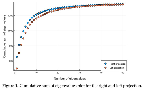
Figure 1.
Cumulative sum of eigenvalues plot for the right and left projection.
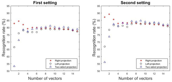
Figure 2.
Recognition rate depending on the number of vectors in the first and second setting for the right, left, and two-sided projection.
Since we used five test images per person, our algorithm could produce individual recognition rates of , , , , , and . The majority of individuals (28 out of 50) were correctly recognized with a recognition rate. Only one person had a recognition rate of . Figure 3 presents this individual’s known and test images. Our algorithm recognized the person only in the first test image. A possible explanation for this low recognition rate is the difference in facial hair between the known and test images. To address this, we made a small adjustment; we swapped the third known image with the fourth test image, ensuring that at least one image with a beard was included in the known set. This modification increased the recognition rate for this individual from to and improved the overall success rate to .
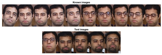
Figure 3.
Ten known images (top) and five test images (bottom) for the only person that had a recognition rate. Our algorithm recognized the person only in the first test image.
5.2. The Second Setting
After observing in the previous subsection that a well-chosen replacement of the test and known images can improve the recognition rate, we conducted a more detailed analysis of the images of five individuals whose recognition rate was . These images are presented in Figure 4. The issue was not facial hair but rather the differences in brightness and skin tones between the test and known images. By making a single switch of images for these five individuals, we increased the overall success rate of the algorithm to . We refer to this new arrangement of images in the database as the second setting. Table 1 presents the number of individuals in each performance category for both settings. The majority of individuals are correctly recognized in all of their test images. Figure 5 showcases examples of individuals with a recognition rate. As observed, our algorithm effectively recognizes faces under varying lighting conditions and skin tones, provided these variations are consistently represented in both the known and test images. Since our recognition process relies on color, it remains sensitive to differences in lighting and skin tone between the known and test images.
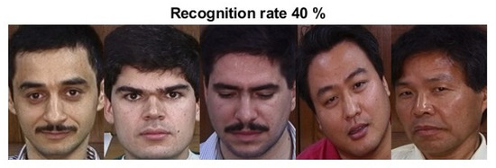
Figure 4.
Images of people with recognition rate in the first setting.

Table 1.
Number of persons per recognition rate in the first and the second setting for our algorithm.
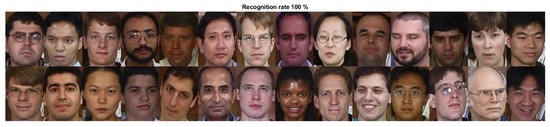
Figure 5.
Images of 28 people for which our algorithm had a 100% recognition rate in the first setting.
For both settings, we tested all three projection types (left, right, and two-sided) to validate the effectiveness of the strategy outlined in Section 4.1. Each algorithm was evaluated using different values of ℓ. The results for both settings are shown in Figure 2. As observed, the best performance is achieved with the proposed projection when . Although the accuracy of other tested projections improves as ℓ increases, they do not reach the level of accuracy obtained using the right projection. Thus, selecting an optimal projection, as described in Section 4.1, enhances accuracy while requiring fewer eigenfaces, ultimately reducing the algorithm’s execution time.
5.3. Comparison with Quaternion PCA and Robust PCA
After a detailed analysis of projection selection, as well as the ℓ parameter, we compared our method with quaternion PCA and Robust PCA (described in Section 4.4). We created two versions of the Robust PCA algorithm. Both begin by performing a low-rank plus sparse decomposition on the entire set of images. In the first version, referred to as Robust PCA, no projections are applied. Instead, recognition is based on directly comparing the low-rank components of the images. The person on the test image is identified by evaluating the norms of the differences between its low-rank component and those of the known images. In the second version (referred to as Robust PCA + Proposed method), we integrated our method with Robust PCA by using the low-rank approximations of the images in place of the original quaternion matrices in Algorithm 1. An example of the low-rank and sparse components reconstructed as images is shown in Figure 6. The low-rank component clearly preserves the most of the features of the original image.
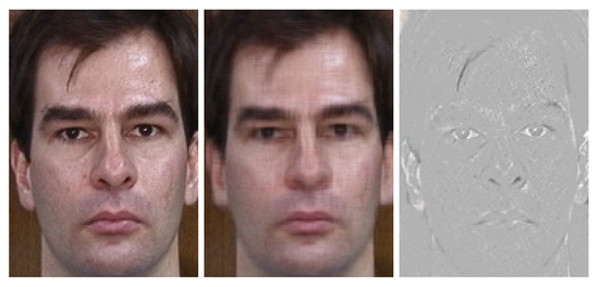
Figure 6.
Original image (left) and its low-rank (middle) and sparse (right) components, obtained using principal component pursuit by alternating directions from Section 4.4.
The results are presented in Table 2. Our proposed method outperforms others in terms of speed while attaining an excellent recognition rate. Although Robust PCA followed by the proposed method yields a similar recognition rate (even slightly better in the first setting), it requires significantly more time. As shown in Table 2, combining Robust PCA with our method results in faster performance compared to using Robust PCA alone. This improvement is due to the use of projected matrices with significantly reduced dimensions when computing the norm of the difference between known and test images.
Table 2.
Recognition rates and execution times for proposed method, PCA, Robust PCA, and Robust PCA followed by the proposed method.
In our implementation of the PCA method, we computed the full singular value decomposition. Although it is possible to accelerate the algorithm by computing a partial singular value decomposition using the Lanczos method, as demonstrated in [7], this approach does not significantly increase speed.
6. Discussion
The effectiveness of our proposed face recognition algorithm is demonstrated by the presented results. Although quaternion-based algorithms have previously been applied to face recognition, our approach introduces an optimal projection selection strategy and a novel Jacobi algorithm to compute the eigenvalues of Hermitian matrices, an essential component of the recognition process. Moreover, we have proven that in the quaternion domain, eigenvectors uniquely solve the problem of maximizing projected images, which is the main foundation of our algorithm. To enhance efficiency and simplicity, we implemented the algorithm in the Julia programming language. Its polymorphic properties enabled the easy implementation of the Jacobi algorithm for quaternion matrices, allowing us to process larger image dimensions () compared to others tested with the quaternion model. The execution time is only a few seconds. For evaluation, we chose the Georgia Tech image database that is often used in similar research and obtained comparable results [6,7,8,12,14]. The recognition rates of other published methods, tested with the same database, are presented in Table 3.
Table 3.
Recognition rates for our proposed method and other published methods.
The algorithms described in [6,8,12,14] rely on the eigenvalue decomposition of the covariance matrix. However, they consider only a single type of matrix, without providing a justification for this choice or evaluating its suitability for the given problem. Furthermore, they do not utilize the eigenvalues to guide the selection of effective projections. In contrast, because of our proof of Theorem 3, we use the plots of the cumulative sums of eigenvalues in Figure 1 of both matrices. They provide a valuable insight into which projection is optimal and how small the value of ℓ can be. In this case, the optimal projection is the one from the right. The results demonstrate the effectiveness of the projection selection strategy in our algorithm. The chosen projection achieves high accuracy with a minimal number of eigenfaces. Although the accuracy of the other two projections (left and two-sided) improves as ℓ increases, they do not reach the level of performance attained by the right projection. This indicates that although increasing ℓ can improve suboptimal projection choices, it does not necessarily lead to the same level of efficiency and accuracy as selecting the optimal projection from the beginning. The smaller number of eigenfaces also reduces the computational load, resulting in faster execution times.
The results presented in Table 2 demonstrate that our proposed method significantly outperforms both PCA and Robust PCA in terms of computational speed, while also maintaining a high recognition rate. Although the combination of Robust PCA with our method achieves a comparable recognition rate, it does so at the cost of longer computation time. This highlights the advantage of our method in balancing accuracy with efficiency.
Testing the algorithm on the original sequence of images from the database, we noticed that it is sensitive to different lighting between the known and test images. However, when we created a second setting in which at least one known image had lighting similar to the test image, the recognition rate increased. This suggests that even better face recognition results could be achieved by introducing a pre-processing step to equalize the lighting between the known and test images.
7. Conclusions
In this paper, we present a quaternion-based algorithm designed to recognize individuals in a given image by identifying the closest match from a known image database. To address the large size of the quaternion matrices representing the images, our algorithm projects them onto a carefully selected subspace, effectively reducing their dimensionality while preserving as much relevant information as possible. We proved that the eigenvectors of the quaternion covariance matrix are the only ones that maximize the Frobenius norm of projected quaternion matrices, serving as the fundamental principle of our approach. The proposed algorithm integrates an efficient projection selection strategy with a novel Jacobi algorithm for the eigenvalue decomposition of Hermitian matrices. Implementation in the Julia programming language ensures low execution time and supports larger image dimensions, enhancing overall efficiency. Testing on a widely used database showed recognition rates comparable to existing studies while using a very small number of eigenvectors. Comparison with PCA and Robust PCA demonstrated that our method offers significantly improved speed and performance.
Author Contributions
Conceptualization, A.C. and I.S.; formal analysis, A.C. and I.S.; funding acquisition, I.S.; investigation, A.C. and I.S.; methodology, A.C. and I.S.; project administration, I.S.; software, A.C. and I.S.; supervision, I.S.; writing—original draft, A.C. and I.S. All authors have read and agreed to the published version of the manuscript.
Funding
This work has been fully supported by the Croatian Science Foundation under the project ‘Matrix Algorithms in Noncommutative Associative Algebras’ (IP-2020-02-2240).
Data Availability Statement
The original contributions presented in this study are included in the article. Further inquiries can be directed to the corresponding author.
Acknowledgments
The authors would like to thank the editor and the reviewers for their valuable comments and suggestions.
Conflicts of Interest
The authors declare no conflicts of interest.
References
- Mukundan, R.; Mukundan, R. Quaternions. In Advanced Methods in Computer Graphics: With Examples in OpenGL; Springer Science & Business Media: Berlin/Heidelberg, Germany, 2012; pp. 77–112. [Google Scholar]
- Lei, X.; Adamo-Villani, N.; Benes, B.; Wang, Z.; Meyer, Z.; Mayer, R.; Lawson, A. Perceived Naturalness of Interpolation Methods for Character Upper Body Animation. In Proceedings of the Advances in Visual Computing: 16th International Symposium, ISVC 2021, Virtual Event, 4–6 October 2021; Proceedings, Part I. Springer: Berlin/Heidelberg, Germany, 2021; pp. 103–115. [Google Scholar]
- Liu, H.; Wang, X.; Zhong, Y. Quaternion-based robust attitude control for uncertain robotic quadrotors. IEEE Trans. Ind. Inform. 2015, 11, 406–415. [Google Scholar] [CrossRef]
- Gołąbek, M.; Welcer, M.; Szczepański, C.; Krawczyk, M.; Zajdel, A.; Borodacz, K. Quaternion attitude control system of highly maneuverable aircraft. Electronics 2022, 11, 3775. [Google Scholar] [CrossRef]
- Chen, Y.; Xiao, X.; Zhou, Y. Low-rank quaternion approximation for color image processing. IEEE Trans. Image Process. 2019, 29, 1426–1439. [Google Scholar] [CrossRef] [PubMed]
- Jia, Z.G.; Ling, S.T.; Zhao, M.X. Color two-dimensional principal component analysis for face recognition based on quaternion model. In Proceedings of the Intelligent Computing Theories and Application: 13th International Conference, ICIC 2017, Liverpool, UK, 7–10 August 2017; Proceedings, Part I 13. Springer: Berlin/Heidelberg, Germany, 2017; pp. 177–189. [Google Scholar]
- Jia, Z.; Ng, M.K.; Song, G.J. Lanczos method for large-scale quaternion singular value decomposition. Numer. Algorithms 2019, 82, 699–717. [Google Scholar] [CrossRef]
- Xiao, X.; Zhou, Y. Two-dimensional quaternion PCA and sparse PCA. IEEE Trans. Neural Netw. Learn. Syst. 2018, 30, 2028–2042. [Google Scholar] [CrossRef] [PubMed]
- Turk, M.; Pentland, A. Eigenfaces for recognition. J. Cogn. Neurosci. 1991, 3, 71–86. [Google Scholar] [CrossRef] [PubMed]
- Yang, J.; Zhang, D.; Frangi, A.F.; Yang, J.y. Two-dimensional PCA: A new approach to appearance-based face representation and recognition. IEEE Trans. Pattern Anal. Mach. Intell. 2004, 26, 131–137. [Google Scholar] [CrossRef] [PubMed]
- Li, L.; Mu, X.; Li, S.; Peng, H. A review of face recognition technology. IEEE Access 2020, 8, 139110–139120. [Google Scholar] [CrossRef]
- Wang, M.; Song, L.; Sun, K.; Jia, Z. F-2D-QPCA: A quaternion principal component analysis method for color face recognition. IEEE Access 2020, 8, 217437–217446. [Google Scholar] [CrossRef]
- Xiao, X.; Zhou, Y. Two-dimensional quaternion sparse principle component analysis. In Proceedings of the 2018 IEEE International Conference on Acoustics, Speech and Signal Processing (ICASSP), Calgary, AB, Canada, 15–20 April 2018; IEEE: Piscataway, NJ, USA, 2018; pp. 1528–1532. [Google Scholar]
- Zhao, M.; Jia, Z.; Gong, D. Improved two-dimensional quaternion principal component analysis. IEEE Access 2019, 7, 79409–79417. [Google Scholar] [CrossRef]
- Badeńska, A.; Błaszczyk, Ł. Compressed sensing for real measurements of quaternion signals. J. Frankl. Inst. 2017, 354, 5753–5769. [Google Scholar] [CrossRef]
- Zhang, F. Quaternions and matrices of quaternions. Linear Algebra Its Appl. 1997, 251, 21–57. [Google Scholar] [CrossRef]
- Farenick, D.R.; Pidkowich, B.A. The spectral theorem in quaternions. Linear Algebra Its Appl. 2003, 371, 75–102. [Google Scholar] [CrossRef]
- Farid, F.; Wang, Q.W.; Zhang, F. On the eigenvalues of quaternion matrices. Lin. Multilin. Alg. 2011, 59, 451–473. [Google Scholar] [CrossRef]
- Ahmad, S.S.; Ali, I.; Slapničar, I. Perturbation analysis of matrices over a quaternion division algebra. Electron. Trans. Numer. Anal. 2021, 54, 128–149. [Google Scholar] [CrossRef]
- Macías-Virgós, E.; Pereira-Sáez, M.; Tarrío-Tobar, A.D. Rayleigh quotient and left eigenvalues of quaternionic matrices. Linear Multilinear Algebra 2023, 71, 2163–2179. [Google Scholar] [CrossRef]
- Jia, Z.; Wei, M.; Ling, S. A new structure-preserving method for quaternion Hermitian eigenvalue problems. J. Comput. Appl. Math. 2013, 239, 12–24. [Google Scholar] [CrossRef]
- Ma, R.R.; Jia, Z.G.; Bai, Z.J. A structure-preserving Jacobi algorithm for quaternion Hermitian eigenvalue problems. Comput. Math. Appl. 2018, 75, 809–820. [Google Scholar] [CrossRef]
- Golub, G.H.; Van Loan, C.F. Matrix Computations; JHU Press: Baltimore, MD, USA, 2013. [Google Scholar]
- Slapničar, I. Symmetric matrix eigenvalue techniques. In Handbook of Linear Algebra; Chapman and Hall/CRC: Boca Raton, FL, USA, 2014; Chapter 55; pp. 1–23. [Google Scholar]
- Candès, E.J.; Li, X.; Ma, Y.; Wright, J. Robust principal component analysis? J. ACM (JACM) 2011, 58, 1–37. [Google Scholar] [CrossRef]
- Demmel, J.W. Applied Numerical Linear Algebra; SIAM: Philadelphia, PA, USA, 1997. [Google Scholar]
- Nefian, A.V. Georgia Tech Face Database. Available online: http://www.anefian.com/research/face_reco.htm (accessed on 10 March 2025).
Disclaimer/Publisher’s Note: The statements, opinions and data contained in all publications are solely those of the individual author(s) and contributor(s) and not of MDPI and/or the editor(s). MDPI and/or the editor(s) disclaim responsibility for any injury to people or property resulting from any ideas, methods, instructions or products referred to in the content. |
© 2025 by the authors. Licensee MDPI, Basel, Switzerland. This article is an open access article distributed under the terms and conditions of the Creative Commons Attribution (CC BY) license (https://creativecommons.org/licenses/by/4.0/).