The Conservative and Efficient Numerical Method of 2-D and 3-D Fractional Nonlinear Schrödinger Equation Using Fast Cosine Transform

Abstract

This paper introduces a novel approach employing the fast cosine transform to tackle the 2-D and 3-D fractional nonlinear Schrödinger equation (fNLSE). The fractional Laplace operator under homogeneous Neumann boundary conditions is first defined through spectral decomposition. The difference matrix Laplace operator is developed by the second-order central finite difference method. Then, we diagonalize the difference matrix based on the properties of Kronecker products. The time discretization employs the Crank–Nicolson method. The conservation of mass and energy is proved for the fully discrete scheme. The advantage of this method is the implementation of the Fast Discrete Cosine Transform (FDCT), which significantly improves computational efficiency. Finally, the accuracy and effectiveness of the method are verified through two-dimensional and three-dimensional numerical experiments, solitons in different dimensions are simulated, and the influence of fractional order on soliton evolution is obtained; that is, the smaller the alpha, the lower the soliton evolution.

1. Introduction

The Nonlinear Schrödinger Equation (NLSE) is a nonlinear partial differential equation that describes the evolution of wave functions in quantum mechanics. It finds extensive applications across various fields of physics, including optics [1], cold atomic physics [2], and plasma physics [3]. In nonlinear optics, the NLSE serves as a fundamental mathematical model to depict the behavior of light waves in nonlinear media. In semiconductor physics, the NLSE describes the propagation of optical solitons in optical fibers made from semiconductor materials [4]. The NLSE is crucial in studying the nonlinear dynamics of semiconductor lasers, particularly in mode-locking and the generation of ultra-short optical pulses [5]. Moreover, it has wide-ranging applications in all-optical communications and all-optical information storage [6]. In recent years, many scholars have introduced fractional-order derivatives into the NLSE, leading to the fractional nonlinear Schrödinger equation (fNLSE). This modification enriches and complicates the dynamical behavior of systems. The fNLSE has been extensively used in various fields such as nonlinear optics [7], Bose–Einstein condensation [8], electromagnetics [9], and quantum mechanics [10]. In nonlinear optics, this equation is employed to describe and predict complex optical phenomena induced by nonlinear effects in optical media, including signal transmission in optical fibers [11], the evolution of wave packets [12], and the interaction among optical solitons [13]. Numerical simulation of solitons through difference equations and exploration of soliton applications in different fields have become hot topics in research. Solitons have been widely applied in various fields such as hydrodynamics [14], dynamics [15,16], ocean engineering [17], etc. Extracting new soliton solutions to study the hidden physical conditions of nonlinear fractional-order partial differential equations has become an important research direction [18,19,20].

We study the following 2-D fNLSE:

$$i\frac{\partial u}{\partial t}(\mathbf{x},t)-{(-\Delta u(\mathbf{x},t\left)\right)}^{\frac{\alpha }{2}}+V\left(\mathbf{x}\right)u(\mathbf{x},t)+\beta {\left|u(\mathbf{x},t)\right|}^{2}u(\mathbf{x},t)=0,\mathbf{x}\in \mathsf{\Omega },t\in (0,T]$$

(1)

where $\mathsf{\Omega }$ represents a 2-D or 3-D with homogeneous Neumann boundary conditions, $u(\mathbf{x},t)$ is a complex function, $i^2=-1$ is the imaginary unit, $V\left(\mathbf{x}\right)$ is the potential function, and $\beta$ is a constant. The symbol ${(-\Delta u)}^{\frac{\alpha }{2}}$ denotes the fractional Laplace operator, where $\alpha$ is a positive real number, and $\alpha =2$ stands for the classical Laplace operator. The fractional Laplace operator can be defined in various ways, commonly through Fourier transform methods, integral representations, fractional Sobolev space approaches, and spectral definitions. Since we discuss the homogeneous Neumann boundaries in this paper, the spectral definition method is adopted as follows [21]:

$${(-\Delta )}^{\frac{\alpha }{2}}u\left(\mathbf{x}\right)=\sum _{k=1}^{\infty }{c}_k{\mu }_k^{\frac{\alpha }{2}}{\phi }_k\left(\mathbf{x}\right),$$

(2)

where ${\mu }_k$ is the eigenvalues of $(-\Delta u)$, and ${\phi }_k$ corresponds to the eigenfunction,

$$c_k={\int }_{\mathsf{\Omega }}u{\phi }_{k}dx$$

(3)

It is well-known that the Nonlinear Schrödinger Equation (NLSE) satisfies the conservation of mass and energy. The development of conservation numerical methods has been a research focus. Numerous scholars have developed various conservation methods. Hendy et al. proposed a method combining finite difference/spectrum and Galerkin–Legendre techniques to solve the coupled nonlinear space–time fractional Schrödinger equation, which exhibits non-smooth solutions in the time domain [22]. Li et al. introduced scalar auxiliary variables to reformulate the Schrödinger equation into a new family of systems. These systems were approximated using the implicit midpoint method, repeated ladder method, and fractional center difference method [23]. Liaqat et al. proposed a novel combinatorial calculation method using the conformable natural transform (CNT) and homotopy perturbation method (HPM) to derive analytical and numerical solutions for the time-fractional suitable Schrödinger equation (TFCSE) [24]. Kaabar et al. defined a new generalized double Laplace transform, coupled with the Adomian decomposition method, to solve the newly formulated nonlinear Schrödinger equation with spatiotemporal dispersion [25]. Zhang [26] investigated the optical soliton solutions of the nonlinear Schrödinger equation with a quintic non-Kerr nonlinear term describing the nonlinear wave state of optical solitons, which is a noteworthy and important model in optical fiber communication. Wang and Huang [27,28] investigated energy-conserving difference schemes combined with Alternating Direction Implicit (ADI) methods. Yang derived a linearized energy-conserving finite difference scheme for a class of nonlinear fractional NLSE equations, studying their energy conservation and convergence properties [29]. Klein et al. proposed a Fourier spectral method for the one-dimensional fractional NLSE [30]. Previous studies mainly focus on Dirichlet boundary conditions and periodic boundary conditions. For the problems with Neumann boundary conditions, to the best of the authors’ knowledge, the relevant papers are limited.

This paper presents a novel, rapid, and conservative method for solving the fractional NLSE under Neumann boundaries in 2-D and 3-D cases. We first develop the difference matrix of the 2-D and 3-D Laplace operators using the finite difference method and then diagonalize the matrix based on the properties of Kronecker products. The difference matrix of the fractional Laplace operator can be obtained by the spectral decomposition. Time discretization employs the Crank–Nicolson method, and the conservation of mass and energy in the fully discrete scheme is proved. The advantage of this method is the implementation of the Fast Discrete Cosine Transform (FDCT). The significant improvement in computational efficiency can be observed in the numerical tests.

This paper is arranged as follows. In Section 2, we discretized 2-D and 3-D Equation (1) by using central difference and the Crank–Nicolson method subsequently. In Section 3, we first introduce the Kronecker operator to simplify the calculation. The conservation of energy and mass of the fully discrete scheme is presented. The implementation of FDCT is discussed in detail in Section 4. In Section 5, we provide numerical examples to verify the efficiency, conservation and accuracy of the method.

2. Numerical Schemes

In this section, the numerical scheme for the 2-D fractional nonlinear Schrödinger equation is first introduced, and then the schemes are generalized to the 3-D domain.

2.1. 2-D Case

In this subsection, the rectangular computing domain $\mathsf{\Omega }=\left[a,b\right]\times \left[c,d\right]$ is considered, where the boundaries are the zero Neumann boundaries. The domain is divided into $N_x\times N_y$ grids. The coordinates of the grid points as follows: specifically, the domain is divided into $N_x\times N_y$ grids by some lines paralleling the axes, where the step size in the x direction is $h_x=\raisebox{1ex}{$\left(b-a\right)$}\!\left/ \!\raisebox{-1ex}{$N_x$}\right.$ and in the y direction is $h_y=\raisebox{1ex}{$\left(d-c\right)$}\!\left/ \!\raisebox{-1ex}{$N_y$}\right.$. Let $u_{j,k}$ be the numerical solution of $u(x,y)$, which are assigned at the center points of the meshes:

$$T_h=\left\{\left.\left(x_j,y_k\right)\right|x_j=a+(j-\frac{1}{2})h_x,y_k=c+(k-\frac{1}{2})h_y,j=1,\cdots N_x,k=1,\cdots N_y\right\}.$$

(4)

Suppose the matrix U for the discrete solution on gird center points, i.e., that $U={\left(u_{j,k}\right)}_{N_x\times N_y}$. Applying the central difference method in the x-direction, we obtain the second-order scheme

$${\left(u_{xx}\right)}_{j,k}\approx \frac{u_{j-1,k}-2u_{j-1,k}+u_{j-1,k}}{h_x^2},j=1,2,3,\cdots N_x-1.$$

To obtain a second-order accurate method, we might introduce another unknown $u_{0,k}$ on the ghost point. For the homogeneous Neumann boundary condition, we can use the centered approximation on the left boundary point to obtain

$$\frac{u_{2,k}-u_{0,k}}{2h_x}=0.$$

The proceeding two equations result in a difference matrix in the x direction,

$$K_x={\left(\begin{array}{cccccc}-1& 1& 0& 0& \cdots & 0\\ 1& -2& 1& 0& \cdots & 0\\ 0& 1& -2& 1& \cdots & 0\\ ⋮& ⋮& \ddots & \ddots & \ddots & ⋮\\ 0& 0& 0& 1& -2& 1\\ 0& 0& 0& 0& 1& -1\end{array}\right)}_{N_x\times N_x},$$

and the difference matrix $K_y$ in the y direction can be obtained similarly. We can now obtain the discrete scheme of the Laplacian operator as:

$${\left(\Delta u\right)}_{j,k}\approx {\left(\frac{1}{h_x^2}{K}_{x}U+\frac{1}{h_y^2}U{K}_y\right)}_{j,k}.$$

(5)

The tridiagonal matrices $K_x$ and $K_y$ can be diagonalized as [31]

$$K_x=S_x{\mathsf{\Lambda }}_x{S}_x^{-1},K_y=S_y{\mathsf{\Lambda }}_y{S}_y^{-1}$$

(6)

Here, the eigenvector matrices $S_x$ and $S_y$ are discrete cosine transform matrices, ${\left(S_x\right)}_{j,k}=cos\frac{j\pi }{N_x}(k-\frac{1}{2}),{\left(S_y\right)}_{j,k}=cos\frac{j\pi }{N_y}(k-\frac{1}{2})$, and both are orthogonal matrices. The matrixes ${\mathsf{\Lambda }}_x$ and ${\mathsf{\Lambda }}_y$ are diagonal matrices consisting of eigenvalues, represented in the following form:

$${\mathsf{\Lambda }}_x=diag\left\{{\lambda }_1,{\lambda }_2,\cdots ,{\lambda }_{N_x}\right\},{\lambda }_j=-2+2cos(j\pi /N_x)$$

$${\mathsf{\Lambda }}_y=diag\left\{{\lambda }_1,{\lambda }_2,\cdots ,{\lambda }_{N_y}\right\},{\lambda }_j=-2+2cos(j\pi /N_y)$$

Next, we will rewrite the discrete scheme (5) in matrix-vector multiplication form by the Kronecker product. The Kronecker product $A\otimes B$ is defined by multiplying each element of matrix A by the entire matrix B:

$$A\otimes B=\left(\begin{array}{cccc}{a}_{11}B& a_{12}B& \cdots & a_{1n}B\\ a_{21}B& a_{22}B& \cdots & a_{2n}B\\ \cdots & \cdots & \cdots & \cdots \\ a_{m1}B& a_{m2}B& \cdots & a_{mn}B\end{array}\right),$$

where $A={\left(a_{ij}\right)}_{m\times n}$ and $B={\left(b_{ij}\right)}_{p\times q}$. Set arrays $U={\left(u_{j,k}\right)}_{N_x\times N_y}$ and vectorize the solution matrix U as

$$\mathcal{U}=Vec\left(U\right)={\left(u_{1,1}{u}_{2,1}\cdots u_{N_x,1},\cdots ,u_{1,N_y}{u}_{2,N_y}\cdots u_{N_x,N_y}\right)}^T.$$

(7)

The elements of the diagonal matrix $\mathcal{V}$ are obtained by vectorizing two-dimensional array V.

Set the matrix $\mathcal{K}=\frac{1}{h_x^2}{K}_x\otimes I_y+I_x\otimes \frac{1}{h_y^2}{K}_y$ by the Kronecker product. Then, the discrete scheme (5) can be rewritten into the matrix-vector multiplication form:

$$\mathcal{K}\mathcal{U}=\left(\frac{1}{h_x^2}{K}_x\otimes I_y+I_x\otimes \frac{1}{h_y^2}{K}_y\right)\mathcal{U}$$

(8)

Here, the matrixes $I_x$, $I_y$ are $N_x$-th and $N_y$-th order identity matrix, respectively. Set the time step $\tau =\frac{T}{N},t_n=n\tau ,(n=0,1,\cdots ,N-1)$. The fully discrete scheme of (1) is obtained by using the Crank–Nicolson method as:

$$i\frac{{\mathcal{U}}^{n+1}-{\mathcal{U}}^n}{\tau }-\left({\left(-\mathcal{K}\right)}^{\frac{\alpha }{2}}-\mathcal{V}\right)\frac{{\mathcal{U}}^{n+1}+{\mathcal{U}}^n}{2}+\frac{\beta }{2}\left({\left|{\mathcal{U}}^{n+1}\right|}^2+{\left|{\mathcal{U}}^n\right|}^2\right)\frac{{\mathcal{U}}^{n+1}+{\mathcal{U}}^n}{2}=0$$

(9)

where ${\mathcal{U}}^n$ and ${\mathcal{U}}^{n+1}$ represent the column vector of $\mathcal{U}$ in Equation (7) at different times t, and the computation of the matrix power ${\left(-\mathcal{K}\right)}^{\frac{\alpha }{2}}$ will be presented in Section 3.

2.2. 3-D Case

Next, we consider the 3-D case. The computation domain $\mathsf{\Omega }=\left[a,b\right]\times \left[c,d\right]\times \left[e,f\right]$ is divided into $N_x\times N_y\times N_z$ grids along the x, y, and z directions, respectively. Use $\left(x_j,y_k,z_l\right)$ to represent the center of the meshes, which is defined similarly as in (4). The time step remains consistent with the 2-D case. Let the 3-D array $\tilde{U}={\left(u_{j,k,l}\right)}_{N_x\times N_y\times N_z}$ represent the numerical solution at $\left(x_j,y_k,z_l\right)$, then vectorize the solution array as:

$$\tilde{\mathcal{U}}=Vec\left(\tilde{U}\right)={\left(u_{1,1,1},\cdots ,u_{1,1,N_z},u_{1,2,1},\cdots ,u_{1,2,N_z},\cdots ,u_{1,N_y,N_z},u_{2,1,1},\cdots ,u_{N_x,N_y,N_z}\right)}^T$$

We apply the second-order central difference scheme in space and the Crank–Nicolson in time for Equation (1) in 3-D. The numerical scheme in the matrix-vector multiplication form can be obtained as:

$$i\frac{{\tilde{\mathcal{U}}}^{n+1}-{\tilde{\mathcal{U}}}^n}{\tau }-\left({\left(-\tilde{\mathcal{K}}\right)}^{\frac{\alpha }{2}}-\tilde{\mathcal{V}}\right)\frac{{\tilde{\mathcal{U}}}^{n+1}+{\tilde{\mathcal{U}}}^n}{2}+\frac{\beta }{2}\left({\left|{\tilde{\mathcal{U}}}^{n+1}\right|}^2+{\left|{\tilde{\mathcal{U}}}^n\right|}^2\right)\frac{{\tilde{\mathcal{U}}}^{n+1}+{\tilde{\mathcal{U}}}^n}{2}=0$$

(10)

The difference matrix is defined as:

$$\tilde{\mathcal{K}}=I_z\otimes I_y\otimes K_x+I_z\otimes K_y\otimes I_x+K_z\otimes I_y\otimes I_x$$

(11)

where $I_z$ is the identity matrix of order $N_z$.

3. Conservation

Before proving the conservative properties of the difference scheme, some notations are first introduced. Let $u,v\in C^{N_x\times N_y}$ be a complex grid function on grids $T_h$ in (4). The inner product is defined as: $(u,v)=h_x{h}_y{\displaystyle \sum _{j=1}^{N_x}}{\displaystyle \sum _{k=1}^{N_y}}{u}_{j,k}\overline{v_{j,k}}$, where $\overline{v_{j,k}}$ is the conjugate of $v_{j,k}$. The definition of the $l^2$-norm of grid function v is $∥v∥=\sqrt{\left(v,v\right)}$. We also define the $l^p$-norm as ${∥v∥}_p={\left(h_x{h}_y{\displaystyle \sum _{j=1}^{N_x}}{\displaystyle \sum _{k=1}^{N_y}}{\left|v_{j,k}\right|}^p\right)}^{\frac{1}{p}},0<p<\infty$. When $p=\infty$, we obtain the $l^{\infty }$-norm ${∥v∥}_{\infty }={\displaystyle \underset{1\le j\le N-1}{\max }}\left|u_{j,k}\right|$. The inner product and $l^p$-norm in the 3-D case can be similarly defined and we omit it here.

The conservation of mass and energy will be proved under the fully discrete scheme (8) and (10). Before proceeding, it is necessary to decompose K in (8). To make the paper self-contained, we first present some important properties of the Kronecker product:

i.

$(A\otimes B)(C\otimes D)=AC\otimes BD$

ii.

${(A\otimes B)}^{-1}=A^{-1}\otimes B^{-1}$

iii.

${(A\otimes B)}^T=A^T\otimes B^T$

iv.

$\left(B^T\otimes A\right)vec\left(X\right)=vec\left(AXB\right)$

Based on the properties of the Kronecker product, we give the following Lemmas.

 Lemma 1. 

The 2-D difference matrix $-\mathcal{K}$ in (8) is symmetric positive definite matrices, and it follows that ${\left(-\mathcal{K}\right)}^{\frac{\alpha }{2}}=L^{T}L$. And the 3-D difference matrix in (11) can also be decomposed as ${\left(-\tilde{\mathcal{K}}\right)}^{\frac{\alpha }{2}}={\tilde{L}}^T\tilde{L}$.

Proof. 

Firstly, we prove the decomposition of the 2-D difference matrix $-\mathcal{K}$. Since the discrete cosine transform matrices $S_x,S_y$ are orthogonal, the matrices $K_x,K_y$ in (5) can be written as $K_x=S_x{\mathsf{\Lambda }}_x{S}_x^T,K_y=S_y{\mathsf{\Lambda }}_y{S}_y^T$. Furthermore, by the properties (ii) and (iii) of the Kronecker product, we have:   

$$\begin{array}{cc}\hfill & \frac{1}{h_x^2}{K}_x\otimes I_y=S_x\frac{1}{h_x^2}{\mathsf{\Lambda }}_x{S}_x^T\otimes I_y=S_x\frac{1}{h_x^2}{\mathsf{\Lambda }}_x{S}_x^T\otimes S_y{I}_y{S}_y^T\hfill \\ \hfill & =\left(S_x\otimes S_y\right)\left(\frac{1}{h_x^2}{\mathsf{\Lambda }}_x{S}_x^T\otimes I_y{S}_y^T\right)=\left(S_x\otimes S_y\right)\left(\frac{1}{h_x^2}{\mathsf{\Lambda }}_x\otimes I_y\right)\left(S_x^T\otimes S_y^T\right)\hfill \\ \hfill & =\left(S_x\otimes S_y\right)\left(\frac{1}{h_x^2}{\mathsf{\Lambda }}_x\otimes I_y\right){\left(S_x\otimes S_y\right)}^T\hfill \end{array}$$

(12)

similarly, we obtain:

$$I_x\otimes \frac{1}{h_y^2}{K}_y=\left(S_x\otimes S_y\right)\left(I_x\otimes \frac{1}{h_y^2}{\mathsf{\Lambda }}_y\right){\left(S_x\otimes S_y\right)}^T.$$

(13)

From the above two equations, we have:

$${\left(-\mathcal{K}\right)}^{\frac{\alpha }{2}}=\left(S_x\otimes S_y\right){\left(-\frac{1}{h_x^2}{\mathsf{\Lambda }}_x\otimes I_y-I_x\otimes \frac{1}{h_y^2}{\mathsf{\Lambda }}_y\right)}^{\frac{\alpha }{2}}{\left(S_x\otimes S_y\right)}^T$$

(14)

It is obvious that $\mathsf{\Lambda }=-\frac{1}{h_x^2}{\mathsf{\Lambda }}_x\otimes I_y-I_x\otimes \frac{1}{h_y^2}{\mathsf{\Lambda }}_y$ is a diagonal matrix with positive diagonal elements. Therefore, we can compute the fractional power of the matrix as ${\left(-\mathcal{K}\right)}^{\frac{\alpha }{2}}=\left(S_x\otimes S_y\right){\mathsf{\Lambda }}^{\frac{\alpha }{4}}{\mathsf{\Lambda }}^{\frac{\alpha }{4}}{\left(S_x\otimes S_y\right)}^T=L^{T}L$, where $L={\mathsf{\Lambda }}^{\frac{\alpha }{4}}{\left(S_x\otimes S_y\right)}^T$.

Next, we consider the decomposition of $-\tilde{\mathcal{K}}$ in (10). Based on the properties (i) and (ii) of the Kronecker product, we have:

$$\begin{array}{c}{I}_z\otimes I_y\otimes G_x=\left(S_z{I}_z{S_z}^T\right)\otimes \left(S_y{I}_y{S_y}^T\right)\otimes \left(S_x{\mathsf{\Lambda }}_x{S_x}^T\right)\hfill \\ \hspace{1em}\hspace{1em}=\left(S_z\otimes S_y\otimes S_x\right)\left(I_z\otimes I_y\otimes {\mathsf{\Lambda }}_x\right)\left({S_z}^T\otimes {S_y}^T\otimes {S_x}^T\right)\hfill \end{array}$$

(15)

A similar computation can be applied to $I_z\otimes G_y\otimes I_x,G_z\otimes I_y\otimes I_x$. Then, we can rewrite $-\tilde{\mathcal{K}}$ as:

$$-\tilde{\mathcal{K}}=\left(S_z\otimes S_y\otimes S_x\right)\tilde{\mathsf{\Lambda }}\left({S_z}^T\otimes {S_y}^T\otimes {S_x}^T\right)$$

(16)

where $\tilde{\mathsf{\Lambda }}=I_z\otimes I_y\otimes \frac{1}{h_x^2}{\mathsf{\Lambda }}_x+I_z\otimes \frac{1}{h_y^2}{\mathsf{\Lambda }}_y\otimes I_x+\frac{1}{h_z^2}{\mathsf{\Lambda }}_z\otimes I_y\otimes I_x$ is a diagonal matrix with positive diagonal elements. The fractional power of the matrix $-\tilde{\mathcal{K}}$ can be decomposed as ${\left(-\tilde{\mathcal{K}}\right)}^{\frac{\alpha }{2}}=\left(S_z\otimes S_y\otimes S_x\right){\tilde{\mathsf{\Lambda }}}^{\frac{\alpha }{4}}{\tilde{\mathsf{\Lambda }}}^{\frac{\alpha }{4}}{\left({S_z}^T\otimes {S_y}^T\otimes {S_x}^T\right)}^T={\tilde{L}}^T\tilde{L}$.    □

Now, we complete Lemma 1. The following proofs in 3-D have analogs for the 2-D case, but the formulas are different, i.e., the formulas in the 3-D case are accompanied by a tilde above them. The proof below does not need to be written for both cases, so we will only present the proofs in the 2-D case. By Lemma 1, Lemma 2 can be readily obtained.

 Lemma 2. 

$\left(L^{T}L\mathcal{U},\mathcal{U}\right)=\left(L\mathcal{U},L\mathcal{U}\right)={∥L\mathcal{U}∥}^2$.

With the $l^2$- and $l^p$-norm, the definitions of mass and energy conservation are given as $Q^n={∥{\mathcal{U}}^n∥}^2$ and $E^n={∥L{\mathcal{U}}^n∥}^2-{∥\mathcal{V}{\mathcal{U}}^n∥}^2-\frac{\beta }{2}{∥{\mathcal{U}}^n∥}^4$, respectively.

 Lemma 3. 

For a complex vector $\mathcal{U}$, the following equation holds:

(1) 

$Im({\left(-\mathcal{K}\right)}^{\frac{\alpha }{2}}{\mathcal{U}}^{n+\frac{1}{2}},{\mathcal{U}}^{n+\frac{1}{2}})=0$

(2) 

$Im\left(\left({\left|{\mathcal{U}}^{n+1}\right|}^2+{\left|{\mathcal{U}}^n\right|}^2\right){\mathcal{U}}^{n+\frac{1}{2}},{\mathcal{U}}^{n+\frac{1}{2}}\right)=0$

(3) 

$Re\left({\left(-\mathcal{K}\right)}^{\frac{\alpha }{2}}{\mathcal{U}}^{n+\frac{1}{2}},{\mathcal{U}}^{n+1}-{\mathcal{U}}^n\right)=\frac{1}{2}\left({∥L{\mathcal{U}}^{n+1}∥}^2-{∥L{\mathcal{U}}^n∥}^2\right)$

(4) 

$Re\left(\frac{\beta }{2}\left({\left|{\mathcal{U}}^{n+1}\right|}^2+{\left|{\mathcal{U}}^n\right|}^2\right){\mathcal{U}}^{n+\frac{1}{2}},{\mathcal{U}}^{n+1}-{\mathcal{U}}^n\right)=\frac{\beta }{4}\left({∥{\mathcal{U}}^{n+1}∥}^4-{∥{\mathcal{U}}^n∥}^4\right)$,

where Re denotes the real part and Im denotes the imaginary part. The proof is straightforward by using Lemma 1 and Lemma 2. For more details, the reader is referred to the existing works in [27].

 Theorem 1. 

The fully discrete format (5) satisfies discrete mass conservation:

$$Q^{n+1}=Q^n=\cdots =Q^0$$

Proof. 

Taking the inner product of both sides of Equation (10) with ${\mathcal{U}}^{n+1}+{\mathcal{U}}^n$ and taking the imaginary part, using Lemma 3 (1) and (2), we have:

$${∥{\mathcal{U}}^{n+1}∥}^2-{∥{\mathcal{U}}^n∥}^2=0$$

$${∥{\mathcal{U}}^{n+1}∥}^2={∥{\mathcal{U}}^n∥}^2$$

Thus, $Q^{n+1}=Q^n$, and the proof is complete by iteration.    □

 Theorem 2. 

The fully discrete format (9) satisfies discrete energy conservation.

$$E^{n+1}=E^n=\cdots =E^0$$

Proof. 

Taking the inner product of both sides of Equation (9) with ${\mathcal{U}}^{n+1}-{\mathcal{U}}^n$ and taking the real part, using Lemma 3 (3) and (4), we have:

$${∥L{\mathcal{U}}^{n+1}∥}^2-{∥{\mathcal{U}}^{n+1}∥}^2-\frac{\beta }{2}{∥{\mathcal{U}}^{n+1}∥}^4={∥L{\mathcal{U}}^n∥}^2-{∥\mathcal{V}{\mathcal{U}}^n∥}^2-\frac{\beta }{2}{∥{\mathcal{U}}^n∥}^4$$

Therefore, we obtain $E^{n+1}=E^n$. This immediately implies discrete energy conservation.    □

4. Fast Implementation

Next, we will give the implementation of the solution of Equation (10). The implementation in 3-D is similar to the 2-D case, so we provide the computation with the 2-D case as an example.

$$\left(\frac{i}{\tau }I-\frac{{\left(-\mathcal{K}\right)}^{\frac{\alpha }{2}}-\mathcal{V}}{2}\right){\mathcal{U}}^{n+1}=\left(\frac{i}{\tau }I+\frac{{\left(-\mathcal{K}\right)}^{\frac{\alpha }{2}}-\mathcal{V}}{2}\right){\mathcal{U}}^n+{\mathcal{F}}_{n+\frac{1}{2}}$$

(17)

where ${\mathcal{F}}_{n+\frac{1}{2}}=-\frac{\beta }{4}\left({\left|{\mathcal{U}}^{n+1}\right|}^2+{\left|{\mathcal{U}}^n\right|}^2\right)\left({\mathcal{U}}^{n+1}+{\mathcal{U}}^n\right)$ and I is the $N_x{N}_y$-th order identity matrix. Equation (17) becomes:

$${\mathcal{U}}^{n+1}=A^{-1}B{\mathcal{U}}^n+A^{-1}{\mathcal{F}}_{n+\frac{1}{2}},$$

(18)

where the matrices A and B are defined as:

$$\begin{array}{cc}& A=\left(S_x\otimes S_y\right)\left(\frac{i}{\tau }I-\frac{1}{2}{\left(-\frac{1}{h_x^2}{\mathsf{\Lambda }}_x\otimes I_y-I_x\otimes \frac{1}{h_y^2}{\mathsf{\Lambda }}_y\right)}^{\frac{\alpha }{2}}+\frac{\mathcal{V}}{2}\right){\left(S_x\otimes S_y\right)}^{-1}\hfill \\ & B=\left(S_x\otimes S_y\right)\left(\frac{i}{\tau }I+\frac{1}{2}{\left(-\frac{1}{h_x^2}{\mathsf{\Lambda }}_x\otimes I_y-I_x\otimes \frac{1}{h_y^2}{\mathsf{\Lambda }}_y\right)}^{\frac{\alpha }{2}}-\frac{\mathcal{V}}{2}\right){\left(S_x\otimes S_y\right)}^{-1}\hfill \end{array}$$

according to Equation (17). We solve the above nonlinear system (18) by Picard iteration. The specific iteration algorithm is as following Algorithm 1 [32]:

Algorithm 1: The Picard iteration for the nonlinear system (18)

$\begin{array}{l}{\mathcal{U}}_0={\mathcal{U}}_0\left(x_j,y_k\right)\hfill \\ forn=0,1,\dots N\hfill \\ {{\mathcal{U}}^0}_{n+1}={\mathcal{U}}_n\hfill \\ forp=1,2\cdots \hfill \\ \begin{array}{cc}& \end{array}{{\mathcal{U}}_{n+1}}^{p+1}=A^{-1}B{\mathcal{U}}^n+A^{-1}\frac{\mathcal{F}({\mathcal{U}}_n)+\mathcal{F}({{\mathcal{U}}_{n+1}}^p)}{2}\hfill \\ \begin{array}{cc}& \end{array}while\left|\right|{{\mathcal{U}}_{n+1}}^{p+1}-{{\mathcal{U}}_{n+1}}^p{\left|\right|}_{\infty }<\epsilon ={10}^{-13}\hfill \\ \begin{array}{c}\end{array}continue\hfill \\ end\hfill \\ {\mathcal{U}}_n={{\mathcal{U}}_{n+1}}^{p+1}\hfill \\ end\hfill \end{array}$

Next, we will use a fast discrete cosine transform to solve Equation (18). Let

$${\mathsf{\Lambda }}_1=\frac{i}{\tau }I-{\left(-\frac{1}{h_x^2}{\mathsf{\Lambda }}_x\otimes I_y-I_x\otimes \frac{1}{h_y^2}{\mathsf{\Lambda }}_y\right)}^{\frac{\alpha }{2}}+\frac{\mathcal{V}}{2},{\mathsf{\Lambda }}_2=\frac{i}{\tau }I+{\left(-\frac{1}{h_x^2}{\mathsf{\Lambda }}_x\otimes I_y-I_x\otimes \frac{1}{h_y^2}{\mathsf{\Lambda }}_y\right)}^{\frac{\alpha }{2}}-\frac{\mathcal{V}}{2}$$

we rewrite Equation (18) as the following equations:

$${\mathcal{U}}^{n+1}=\left(S_x\otimes S_y\right)\left({\mathsf{\Lambda }}_1^{-1}{\mathsf{\Lambda }}_2\right){\left(S_x\otimes S_y\right)}^{-1}{\mathcal{U}}^n+\left(S_x\otimes S_y\right){\mathsf{\Lambda }}_1^{-1}{\left(S_x\otimes S_y\right)}^{-1}{\mathcal{F}}_{n+\frac{1}{2}}$$

(19)

Due to the similarity in computation steps between the two terms on the right-hand side of Equation (19), we take the second term as an example. The computational procedure is divided into three steps:

Step 1:

According to the properties of the Kronecker product (ii) and (iv), the matrix-vector multiplication of ${\left(S_x\otimes S_y\right)}^{-1}F$ in Equation (17) can be achieved as follows:

$${\left(S_x\otimes S_y\right)}^{-1}vec\left(F\right)=\left(S_x^{-1}\otimes S_y^{-1}\right)vec\left(F\right)=vec\left(S_y^{-1}F{S}_x\right)$$

It can be achieved using the fast discrete cosine transform.

Step 2:

Since it is a diagonal matrix, ${\mathsf{\Lambda }}_1^{-1}vec\left(S_y^{-1}F{S}_x\right)=vec\left(S_y^{-1}F{S}_x./\mathsf{\Lambda }\right)$, where ${\mathsf{\Lambda }}^{-1}$ is represented by $./\mathsf{\Lambda }$.

Step 3:

Since $S_x=S_x^T$, then $\left(S_x\otimes S_y\right)vec\left(S_y^{-1}F{S}_x./\mathsf{\Lambda }\right)=vec\left(S_y\left(S_y^{-1}F{S}_x./\mathsf{\Lambda }\right)S_x\right)$. This part can be achieved using the fast inverse discrete cosine transform.

5. Numerical Experiments and Discussion

5.1. Numerical Experiments

In this section, we report some numerical results of the 2-D and 3-D fNLS Equation (1) to support our theoretical analysis.

 Example 1. 

We consider the problem (1) in $\mathsf{\Omega }=\left[-\pi ,\pi \right]\times \left[-\pi ,\pi \right]$, with the potential function $V(x,y)=1-4{\cos }^{2}2x{\sin }^{2}2y$. When $\alpha =2$, the problem collapses to the classical cubic nonlinear Schrödinger equation, and the exact solution is given by $u(x,y,t)=e^{9it}\cos 2x\sin 2y$. In this example, we compute the $l^{\infty }$-norm errors $e(\tau ,h)={∥u\left(T\right)-U^{N_t}∥}_{\infty }$ of the numerical solution at T = 1. The time step is fixed with a small time step, $\tau =1\times {10}^{-4}$.

Firstly, we test the discrete mass conservation law. Figure 1 gives the evolution of mass Qn and energy En for 1.6, 1.7, 1.8, 2, respectively, with $\tau$ = h = 0.01.

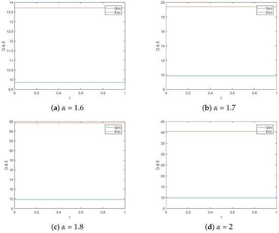
Figure 1. The evolution of discrete mass and energy for different values of $\alpha$.

In Table 1, we compute the maximum norm errors of the energy and mass of the numerical solution with $\tau =h=0.01$ at $t=1$, which helps to better evaluate the accuracy and stability of the numerical method. Then, the accuracy of the example is demonstrated by computing the error between the analytical solution and the numerical solution, with the results presented in Table 2. Table 2 shows that the scheme has second-order accuracy in space. It is worth noting that the scheme with DCT performs the computation in CPU time, which is several orders of magnitude shorter with respect to the no DCT method. Table 3 is obtained by scheme (9) with different time steps. The spatial step is also chosen to be relatively small (h = 0.05). The results from Table 3 indicate that our scheme is second-order in time.

Table 1. The maximal errors of the energy and mass with $\tau =h=0.01$ at $t=1$.

$\mathit{\alpha }$	E(n)	Q(n)
1.6	2.46 $\times {10}^{-12}$	2.27 $\times {10}^{-12}$
1.7	2.52 $\times {10}^{-12}$	3.40 $\times {10}^{-12}$
1.8	2.61 $\times {10}^{-12}$	4.82 $\times {10}^{-12}$
2	2.98 $\times {10}^{-12}$	8.79 $\times {10}^{-12}$

Table 2. The error and CPU with $T=1$ and $\tau =1\times {10}^{-4}$.

DCT	N	32	64	128	256
	Error	2.6 $\times {10}^{-3}$	6.42 $\times {10}^{-4}$	1.61 $\times {10}^{-4}$	4.02 $\times {10}^{-5}$
	CPU(s)	0.2	0.4	1.63	4.12
NO DCT	N	32	64	128	256
	Error	2.6 $\times {10}^{-3}$	6.42 $\times {10}^{-4}$	6.42 $\times {10}^{-4}$	-
	CPU(s)	1.97	52.36	1815.55	-

Table 3. Order of convergence in terms of time.

$\mathit{\tau }$	a = 1.8	a = 1.9	a = 2.0
	e($\mathit{\tau }$)	e($\mathit{\tau }$)	e($\mathit{\tau }$)
1/100	1.49 $\times {10}^{-3}$	8.19 $\times {10}^{-4}$	7.67 $\times {10}^{-4}$
1/200	3.73 $\times {10}^{-4}$	2.06 $\times {10}^{-4}$	1.92 $\times {10}^{-4}$
1/400	9.32 $\times {10}^{-5}$	5.12 $\times {10}^{-5}$	4.82 $\times {10}^{-5}$
1/800	2.26 $\times {10}^{-5}$	1.28 $\times {10}^{-5}$	1.20 $\times {10}^{-5}$

 Example 2. 

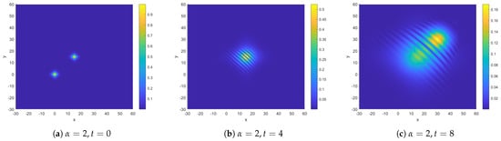
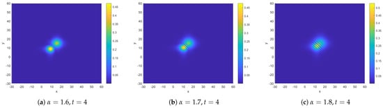
Now, we investigate the impact of the collision of two solitons brought by fractional order. In this example, we compute the interaction between two solitons. Take $V(x,y)=0,\beta =2$ and $\mathsf{\Omega }=[-30,60]\times [-30,60]$ in (1). The initial conditions are given as follows: $u(x,y,0)=e^{2i(x+y)}sechxsechy+e^{0.05i(x+y-15)}sech(x-15)sech(y-15).$ In order to illustrate the fact clearly, we first specify the elastic collisions with $\alpha =2.0$. It can be observed that the waves retain their shape and velocity after interaction (see Figure 2). Then, we choose different α to test the collisions of two solitons. Figure 3 shows the evolution of the modulus of the collision at $t=4$ for $\alpha =1.6,1.7,1.8$, respectively. We can find that the order α will greatly affect the collision time. The smaller α becomes, the longer the collision time. Generally, a reduction in the order may indicate a stronger memory effect in the system, leading to a slower interaction between isolated solitons. This feature is consistent with the fact that the fractional order introduces more historical information.

Figure 2. The interaction between two solitons at different times with $\alpha =2,\tau =0.01$.

Figure 3. The interactions between two solitons at different times with $\alpha =1.6,\alpha =1.7,\alpha =1.8$.

 Example 3. 

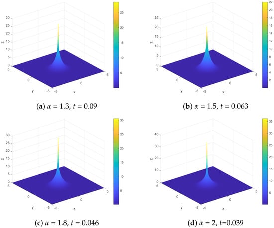
The solutions of the nonlinear Schrödinger equation can exhibit a phenomenon known as ‘blow-up’. In this example, we show the singular solutions for the FNLS equation. We choose $V(x,y)=0,\beta =1$ and $\mathsf{\Omega }=[-10,10]\times [-10,10]$ in (1). The initial condition is $u(x,y,0)=6\sqrt{2}exp(-(x^2+y^2))$. Figure 4 shows the modulus of the solution $\left|u(x,y)\right|$ with different fractional order, $\alpha =1.3,\alpha =1.5,\alpha =1.8,\alpha =2.0$. The blow-up effect is obtained in finite time with different α. These plots show that the blow-up time becomes smaller for progressively increasing α. This is because the fractional-order derivatives introduce a dependence on the system’s past states, causing the evolution of the system to be influenced by previous states over longer distances.

Figure 4. The modulus of solution in Example 3 with different $\alpha$ and blow-up time.

 Example 4. 

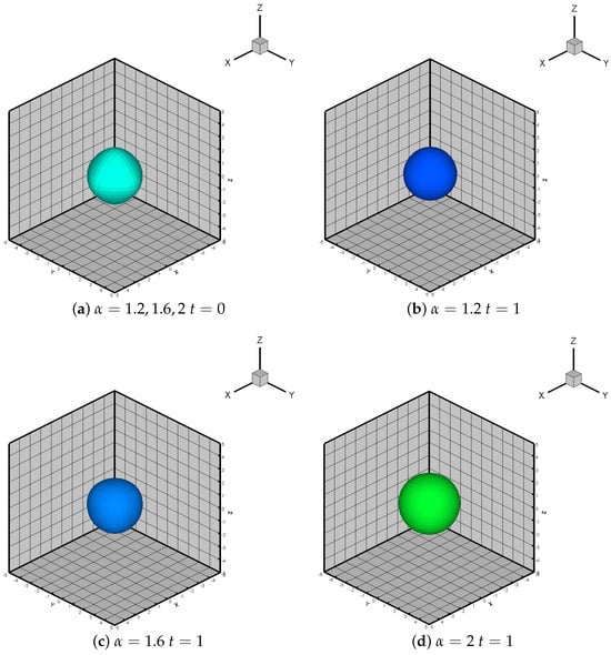
Finally, we consider the 3-D problem (1) in $\mathsf{\Omega }={[-10,10]}^3$, with $V(x,y)=0,\beta =2$. We set the final computation time as t = 1. The initial conditions are $u(x,y,z,0)=sech\left(x\right)sech\left(y\right)sech\left(z\right)exp\left(i\right(x+y+z\left)\right)$. To better illustrate the results, Figure 5 describes the time evolutions of solitons. Figure 5a shows the initial solution with the isosurfaces $\left|u\right|=0.25$. Figure 5b–d demonstrate the solution of $\left|u\right|=0.25$, where the fractional orders are chosen as $\alpha =1.2,1.6,$ and 2. It can be seen from the figure that the order α will greatly affect the soliton. The soliton propagates at a slower speed when α decreases.

Figure 5. The evolution of the soliton in 3-D with different fractional order.

5.2. Discussion

In Figure 1, the conservation of mass E and energy Q is clearly depicted, alongside the discernible trend that, under varying $\alpha$, the mass remains nearly constant while the energy Q decreases with $\alpha$. Figure 2 presents simulation diagrams illustrating optical solitons with integer orders at different time intervals. These diagrams vividly show the loss and diffraction phenomena occurring during the propagation of optical solitons. By comparing with Figure 2, Figure 3 elucidates the influence of $\alpha$ on the motion of optical solitons: as $\alpha$ decreases, the propagation speed of optical solitons decelerates. The occurrence of blasting phenomena significantly impacts the stability of optical soliton propagation. In Figure 4, the blasting time for different $\alpha$ when solving the Schrödinger equation is demonstrated. To accentuate the blasting phenomenon, a three-dimensional image is provided for better observation, revealing that smaller $\alpha$ results in slower blasting phenomena. Figure 5 presents the isosurface diagram concerning u, offering a theoretical foundation for the study of optical solitons.

6. Conclusions

This paper solves the two-dimensional and three-dimensional fractional nonlinear Schrödinger equation under the Neumann boundaries. Our scheme employs Kronecker products to represent the differential matrix of the fully discrete equation. This is more helpful for our proof of the conservation of mass and energy. In addition, it obviously improves the computing speed. In the implementation process, the application of the Fast Discrete Cosine Transform effectively reduces computation time. Furthermore, extensive numerical experiments in the 2-D case and the 3-D case are given to confirm the method’s accuracy, efficiency, and stability. By varying fractional order, we could observe the impact of fractional order. Specifically, we noted that the smaller the fractional order, the slower the movement and formation of optical solitons. Furthermore, the approach delineated in this article extends its applicability beyond the specific differential equation under consideration. It not only serves to verify the conservation properties of various other differential equations but also introduces an innovative methodology for their solutions. This provides a theoretical basis for the study of optical soliton propagation in optical fibers and nonlinear optics. This highlights the need for further study in the future.

7. Future Work

In the future, we will focus on the study of nonlinear optical solitons depicted by different differential equations and extend the methodology to other nonlinear models.

References

- Ibarra-Villalon, H.E.; Pottiez, O.; Gómez-Vieyra, A.; Lauterio-Cruz, J.P.; Bracamontes-Rodriguez, Y.E. Numerical approaches for solving the nonlinear Schrödinger equation in the nonlinear fiber optics formalism. J. Opt. 2020, 22, 043501. [Google Scholar] [CrossRef]
- Vowe, S.; Lämmerzahl, C.; Krutzik, M. Detecting a logarithmic nonlinearity in the Schrödinger equation using Bose-Einstein condensates. Phys. Rev. A 2020, 101, 043617. [Google Scholar] [CrossRef]
- Sultana, S. Review of heavy-nucleus-acoustic nonlinear structures in cold degenerate plasmas. Rev. Mod. Plasma Phys. 2022, 6, 6. [Google Scholar] [CrossRef]
- Rao, J.-G.; Chen, S.-A.; Wu, Z.-J.; He, J.-S. General higher-order rogue waves in the space-shifted symmetric nonlocal nonlinear Schrödinger equation. Acta Phys. Sin. 2023, 72, 104204-1–104204-9. [Google Scholar] [CrossRef]
- Li, M.; Wang, B.T.; Xu, T.; Shui, J.J. Study on the generation mechanism of bright and dark solitary waves and rogue wave for a fourth-order dispersive nonlinear Schrödinger equation. Acta Phys. Sin. 2020, 69, 010502-1–010502-10. [Google Scholar] [CrossRef]
- Wen, J.-M.; Bo, W.-B.; Wen, X.-K.; Dai, C.-Q. Multipole vector solitons in coupled nonlinear Schrödinger equation with saturable nonlinearity. Acta Phys. Sin. 2023, 72, 100502-1–100502-7. [Google Scholar] [CrossRef]
- Ahmad, J.; Akram, S.; Noor, K.; Nadeem, M.; Bucur, A.; Alsayaad, Y. Soliton solutions of fractional extended nonlinear Schrödinger equation arising in plasma physics and nonlinear optical fiber. Sci. Rep. 2023, 13, 10877. [Google Scholar] [CrossRef] [PubMed]
- Jiang, T.; Huang, J.-J.; Lu, L.-G.; Ren, J.-L. Numerical study of nonlinear Schrödinger equation with high-order split-step corrected smoothed particle hydrodynamics method. Acta Phys. Sin. 2019, 68, 090203-1–090203-14. [Google Scholar] [CrossRef]
- Qureshi, S.; Chang, M.M.; Shaikh, A.A. Analysis of series RL and RC circuits with time-invariant source using truncated M, Atangana beta and conformable derivatives. J. Ocean Eng. Sci. 2021, 6, 217–227. [Google Scholar] [CrossRef]
- Stephanovich, V.A.; Olchawa, W.; Kirichenko, E.V.; Dugaev, V.K. 1D solitons in cubic-quintic fractional nonlinear Schrödinger model. Sci. Rep. 2022, 12, 15031. [Google Scholar] [CrossRef] [PubMed]
- Islam, Z.; Abdeljabbar, A.; Sheikh, M.A.N.; Taher, M.A. Optical solitons to the fractional order nonlinear complex model for wave packet envelope. Results Phys. 2022, 43, 106095. [Google Scholar] [CrossRef]
- Xie, P.; Zhu, Y. Wave Packets in the Fractional Nonlinear Schrödinger Equation with a Honeycomb Potential. Multiscale Model. Simul. 2021, 19, 951–979. [Google Scholar] [CrossRef]
- Riaz, M.B.; Atangana, A.; Jahngeer, A.; Jarad, F.; Awrejcewicz, J. New optical solitons of fractional nonlinear Schrodinger equation with the oscillating nonlinear coefficient: A comparative study. Results Phys. 2022, 37, 105471. [Google Scholar] [CrossRef]
- Shahen, N.H.M.; Rahman, M.M. Dispersive solitary wave structures with MI Analysis to the unidirectional DGH equation via the unified method. Partial Differ. Equ. Appl. Math. 2022, 6, 100444. [Google Scholar]
- An, T.; Shahen, N.H.M.; Ananna, S.N.; Hossain, M.F.; Muazu, T. Exact and explicit travelling-wave solutions to the family of new 3D fractional WBBM equations in mathematical physics. Results Phys. 2020, 19, 103517. [Google Scholar]
- Shahen, N.H.M.; Rahman, M.M.; Alshomrani, A.S.; Inc, M. On fractional order computational solutions of low-pass electrical transmission line model with the sense of conformable derivative. Alex. Eng. J. 2023, 81, 87–100. [Google Scholar]
- Iqbal, M.A.; Miah, M.M.; Ali, H.S.; Shahen, N.H.M.; Deifalla, A. New applications of the fractional derivative to extract abundant soliton solutions of the fractional order PDEs in mathematics physics. Partial Differ. Equ. Appl. Math. 2024, 9, 100597. [Google Scholar] [CrossRef]
- Justin, M.; David, V.; Shahen, N.H.M.; Sylvere, A.S. Sundry optical solitons and modulational instability in Sasa-Satsuma model. Opt. Quantum Electron. 2022, 54, 1–15. [Google Scholar] [CrossRef]
- Shahen, N.H.M.; Ali, M.S.; Rahman, M.M. Interaction among lump, periodic, and kink solutions with dynamical analysis to the conformable time-fractional Phi-four equation. Partial Differ. Equ. Appl. Math. 2021, 4, 100038. [Google Scholar] [CrossRef]
- Shahen, N.H.M.; Foyjonnesa Bashar, M.H.; Tahseen, T.; Hossain, S. Solitary and rogue wave solutions to the conformable time fractional modified kawahara equation in mathematical physics. Adv. Math. Phys. 2021, 2021, 6668092. [Google Scholar] [CrossRef]
- Lischke, A.; Pang, G.; Gulian, M.; Song, F.; Glusa, C.; Zheng, X.; Mao, Z.; Cai, W.; Meerschaert, M.M.; Ainsworth, M.; et al. What is the fractional Laplacian? A comparative review with new results. J. Comput. Phys. 2020, 404, 109009. [Google Scholar] [CrossRef]
- Hendy, A.S.; Zaky, M.A. Combined Galerkin spectral/finite difference method over graded meshes for the generalized nonlinear fractional Schrödinger equation. Nonlinear Dyn. 2021, 103, 2493–2507. [Google Scholar] [CrossRef]
- Li, X.; Wen, J.; Li, D. Mass-and energy-conserving difference schemes for nonlinear fractional Schrödinger equations. Appl. Math. Lett. 2021, 111, 106686. [Google Scholar] [CrossRef]
- Liaqat, M.I.; Akgül, A. A novel approach for solving linear and nonlinear time-fractional Schrödinger equations. Chaos Solitons Fractals 2022, 162, 112487. [Google Scholar] [CrossRef]
- Kaabar, M.K.; Martínez, F.; Gómez-Aguilar, J.F.; Ghanbari, B.; Kaplan, M.; Günerhan, H. New approximate analytical solutions for the nonlinear frac-tional Schrödinger equation with second-order spatio-temporal dispersion via double Laplace transform method. Math. Methods Appl. Sci. 2021, 44, 11138–11156. [Google Scholar] [CrossRef]
- Zhang, K.; Han, T. The optical soliton solutions of nonlinear Schrödinger equation with quintic non-Kerr nonlinear term. Results Phys. 2023, 48, 106397. [Google Scholar] [CrossRef]
- Wang, P.; Huang, C. An energy conservative difference scheme for the nonlinear fractional Schrödinger equations. J. Comput. Phys. 2015, 293, 238–251. [Google Scholar] [CrossRef]
- Wang, P.; Huang, C. Split-step alternating direction implicit difference scheme for the fractional Schrödinger equation in two dimensions. Comput. Math. Appl. 2016, 71, 1114–1128. [Google Scholar] [CrossRef]
- Yang, Z. A class of linearized energy-conserved finite difference schemes for nonlinear space-fractional Schrödinger equations. Int. J. Comput. Math. 2016, 93, 609–626. [Google Scholar] [CrossRef]
- Klein, C.; Sparber, C.; Markowich, P. Numerical study of fractional nonlinear Schrödinger equations. Proc. Math. Phys. Eng. Sci. 2014, 470, 20140364. [Google Scholar] [CrossRef]
- LeVeque, R.J. Finite Difference Methods for Ordinary and Partial Differential Equations: Steady-State and Time-Dependent Problems; SIAM: Philadelphia, PA, USA, 2007. [Google Scholar]
- Chen, Z.; Gou, Q. Piecewise Picard iteration method for solving nonlinear fractional differential equation with proportional delays. Appl. Math. Comput. 2019, 348, 465–478. [Google Scholar] [CrossRef]
Disclaimer/Publisher’s Note: The statements, opinions and data contained in all publications are solely those of the individual author(s) and contributor(s) and not of MDPI and/or the editor(s). MDPI and/or the editor(s) disclaim responsibility for any injury to people or property resulting from any ideas, methods, instructions or products referred to in the content. |
© 2024 by the authors. Licensee MDPI, Basel, Switzerland. This article is an open access article distributed under the terms and conditions of the Creative Commons Attribution (CC BY) license (https://creativecommons.org/licenses/by/4.0/).