Stochastic Orderings between Two Finite Mixtures with Inverted-Kumaraswamy Distributed Components

Abstract

In this paper, we consider two finite mixture models (FMMs) with inverted-Kumaraswamy distributed components’ lifetimes. Several stochastic ordering results between the FMMs are obtained. Mainly, we focus on three different cases in terms of the heterogeneity of parameters. The usual stochastic order between the FMMs is established when heterogeneity presents in one parameter as well as two parameters. In addition, we also study ageing faster order in terms of the reversed hazard rate between two FMMs when heterogeneity is in two parameters. For the case of heterogeneity in three parameters, we obtain the comparison results based on reversed hazard rate and likelihood ratio orders. The theoretical developments are illustrated using several examples and counterexamples.

1. Introduction

The FMMs have been widely used in many study areas, including biology, reliability, and survival analysis. As a result, both theorists and practitioners have shown a great deal of interest in these models. Due to its unique ability to model heterogeneous data, whose pattern cannot be produced by a single parametric distribution, the mixture model (MM) has acquired a lot of appeal. An unknown model is developed by mixing a collection of homogeneous subpopulations (infinite) in order to capture this heterogeneity. Keep in mind that the mixing is carried out over a latent parameter, which is regarded as a random variable (RV) and chosen from an unknown mixing distribution. Here, we refer to it as mixing proportions or weights throughout this paper. There are many circumstances in which FMMs spontaneously occur. For more information on the different applications of FMMs, see [1,2,3,4]. For instance,

• An FMM can be used in reliability theory to model the “failure time” of a system. The model assumes that the “failure time” is a mixture of two or more distributions, as usually there is more than one reason causing the failures of a component or system [3].
• To study the distribution of time to death after a major cardiovascular surgery, FMMs are useful. Here, one may consider that the lifetime of such patients after surgery contains three phases of time. In the first phase, that is, immediately after surgery, the death risk is relatively high. In the next phase, the hazard rate remains constant up to some certain time. Then, in the final phase, the risk of death of the patient increases. The convenient way to model this situation is to adopt an MM with three components. In each phase, a separate parametric model can be assigned to each (here, three) component [2].
• An FMM can be used in biological sciences to model the distribution of gene expression levels across different cell types. The model assumes that the gene expression levels are a mixture of two or more distributions, such as a normal distribution and a gamma distribution [2,5].

Also, FMMs are used in a variety of real-life applications, such as clustering, image segmentation, anomaly detection, and speech recognition. They are also used in medical diagnosis, market segmentation, customer segmentation, etc. In this paper, we considered two FMMs for inverted-Kumaraswamy ($\mathcal{IK}$) distributed components.

The topic of stochastic comparisons between two FMMs has been extensively studied. For more details, see [3,6,7,8] and so on. Ref. [9] studied stochastic comparisons of finite mixtures (FMs) where the subpopulations are from semiparametric models, that is, the scale model, proportional hazard rate model, and proportional reversed hazard rate model. Ref. [10] focused on two finite $\alpha$-MMs and established sufficient conditions for comparing two $\alpha$-MRVs. Please see Ref. [11] for some properties of the $\alpha$-MM. Ref. [12] investigated MMs with generalized Lehmann distributed components and presented several ordering outcomes. Ref. [13] studied two FMMs with location-scale family distributed components and established some stochastic comparison results between them in terms of the usual stochastic order and the reversed hazard rate order. By utilizing the majorization idea, Ref. [14] studied a stochastic comparison for two FMs in terms of the usual stochastic order, hazard rate order, and reversed hazard rate order. Ref. [15] established ordering results between two finite mixture random variables (FMRVs), where the mixing components are based on proportional odds, proportional hazards, and proportional reversed hazards models. Ref. [16] obtained some ordering results between two FMMs considering general parametric families of distributions. Mainly, the authors established sufficient conditions for the usual stochastic order based on p-larger order and reciprocally majorization order. Very recently, Ref. [17] considered similar general parametric families of distributions as in [16] and then examined various ordering results with respect to the usual stochastic order, hazard rate order, and reversed hazard rate order between two FMMs.

Inverted distributions have several applications in various fields, including econometrics, life testing, biology, engineering sciences, and medicine. Additionally, it is used in reliability theory, survival analysis, the financial literature, and environmental research. For more details on inverted distributions and their applications, see [18]. Ref. [19] developed the $\mathcal{IK}$ distribution by using the transformation $x=t^{-1}-1$ from the Kumaraswamy ($\mathcal{K}$) distribution, that is, $T\sim \mathcal{K}(\alpha ,\beta )$, where $\alpha$ and $\beta$ are the shape parameters. Then X has an $\mathcal{IK}$ distribution with cdf and pdf as

$$\begin{array}{c}\hfill F_X\left(x\right)\equiv F(x;\alpha ,\beta )={(1-{(1+x)}^{-\alpha })}^{\beta },x>0,\alpha >0,\beta >0\end{array}$$

(1)

and

$$\begin{array}{c}\hfill f_X\left(x\right)\equiv f(x;\alpha ,\beta )=\alpha \beta {(1+x)}^{-\alpha -1}{(1-{(1+x)}^{-\alpha })}^{\beta -1},x>0,\alpha >0,\beta >0,\end{array}$$

(2)

respectively, where $\alpha$ and $\beta$ are both shape parameters. We note that the curves of the pdf and hazard function show that the $\mathcal{IK}$ distribution exhibits a long right tail compared with other commonly used distributions. As a result, it affects long-term reliability predictions, producing optimistic predictions of rare events occurring in the right tail of the distribution compared with other well-known distributions. Here, we use the notation $X\sim \mathcal{IK}(\alpha ,\beta )$ for convenience. Many well-known distributions fall under the $\mathcal{IK}$ distribution as special cases, e.g., the Lomax distribution (for $\beta =1$), beta Type II distribution (for $\alpha =1$) and the log-logistic distribution (for $\alpha =\beta =1$) [19]. Also, using appropriate transformations, the $\mathcal{IK}$ distribution can be transformed to many well-known distributions, such as the exponentiated exponential and Weibull, generalized uniform, generalized Lomax, beta Type II and F-distribution, Burr Type III, and log-logistic distributions [19]. $\mathcal{IK}$ distribution fits those real data.

This paper focuses on the stochastic comparison results between two finite mixture models following $\mathcal{IK}$ distributed components. The goal of this paper is to obtain sufficient conditions for which two finite mixture random variables with $\mathcal{IK}$ distributed component lifetimes are comparable in the sense of the usual stochastic order, reversed hazard rate order, likelihood ratio order, and ageing faster order in terms of reversed hazard rate order.

The main contributions and organization of the paper are as follows. In the next section, we present several definitions and lemmas that are essential to obtain our main results. Section 3 contains three subsections, with a description on the proposed model. In Section 3.1, we establish the usual stochastic order between two FMMs based on the concepts of the weak supermajorization and weak submajorization orders. Section 3.2 deals with the ordering results when there is heterogeneity in two parameters. Here, we obtain comparison results with respect to the usual stochastic order and ageing faster order in terms of the reversed hazard rate. In Section 3.3, we examine ordering results between the FMMs with respect to the reversed hazard rate and likelihood ratio orders. Besides the theoretical contributions, we present many examples and counterexamples for the validation and justification.

Throughout the paper, the term “increasing” refers to “nondecreasing”, while the term “decreasing” will mean “nonincreasing”. For any differentiable function $\eta (·)$, we write ${\eta }^{\prime }\left(t\right)$ to represent the first-order derivative of $\eta \left(t\right)$ with respect to t. The partial derivative of $\xi \left(\mathit{x}\right)$ with respect to its kth component is denoted as “${\xi }_{\left(k\right)}\left(\mathit{x}\right)=\partial \xi \left(\mathit{x}\right)/\partial x_k$” for $k=1,\dots ,n$. Also, “$\stackrel{sign}{=}$” is used to indicate that the signs on both sides of an equality are the same. We use the notation $\mathbb{R}=(-\infty ,+\infty )$, ${\mathbb{R}}^{+}=[0,+\infty )$, ${\mathbb{R}}_n={(-\infty ,+\infty )}^n$, and ${\mathbb{R}}_n^{+}={[0,+\infty )}^n$, respectively.

2. The Basic Definitions and Some Prerequisites

This section presents some preliminary definitions and results, which are essential to establish our main results in the subsequent section. Let U and V be two continuous and non-negative independent random variables with pdfs $f_U(·)$ and $g_V(·)$, cdfs $F_U(·)$ and $G_V(·)$, sfs ${\overline{F}}_U(·)=1-F_U(·)$ and ${\overline{G}}_V(·)=1-G_V(·)$, and rhs ${\tilde{r}}_U(·)=f_U(·)/F_U(·)$ and ${\tilde{r}}_V(·)=g_V(·)/G_V(·)$, respectively.

Definition 1.

The random variable U is smaller than V in the sense of

(i)

usual stochastic order (abbreviated as $U{\le }_{st}V$), if ${\overline{F}}_U\left(x\right)\le {\overline{G}}_V\left(x\right)$ for all $x\in {\mathbb{R}}^{+}$;

(ii)

reversed hazard rate order (abbreviated as $U{\le }_{rh}V$), if $G_V\left(x\right)/F_U\left(x\right)$ is increasing in x for all $x\in {\mathbb{R}}^{+}$; or, equivalently, if ${\tilde{r}}_U\left(x\right)\le {\tilde{r}}_V\left(x\right)$ for all $x\in {\mathbb{R}}^{+}$;

(iii)

likelihood ratio order (abbreviated as $U{\le }_{lr}V$), if $g_V\left(x\right)/f_U\left(x\right)$ is increasing in x for all $x\in {\mathbb{R}}^{+}$;

(iv)

ageing faster order with respect to reversed hazard rate order (abbreviated as $U{\le }_{R-rh}V$), if ${\tilde{r}}_U\left(x\right)/{\tilde{r}}_V\left(x\right)$ is decreasing in x for all $x\in {\mathbb{R}}^{+}$.

It is important to note that $U{\le }_{lr}V\Rightarrow U{\le }_{rh}V\Rightarrow U{\le }_{st}V$. Ref. [6] provides a comprehensive overview of stochastic orders and their applications. The idea of majorization and related orders are then discussed, which are highly helpful in establishing the main results in the subsequent sections. Let ${\mathbb{R}}_n$ be an n-dimensional Euclidean space. Let $\mathit{\varsigma }=({\varsigma }_1,\dots ,{\varsigma }_n)$ and $\mathit{\epsilon }=({\epsilon }_1,\dots ,{\epsilon }_n)$ be two real vectors. Further, let ${\varsigma }_{\left(1\right)}\le \dots \le {\varsigma }_{\left(n\right)}$ and ${\epsilon }_{\left(1\right)}\le \dots \le {\epsilon }_{\left(n\right)}$ denote the increasing arrangements of the components of the vectors $\mathit{\varsigma }$ and $\mathit{\epsilon }$, respectively.

Definition 2

([20]). The vector ς is said to

• majorize the vector ε (abbreviated as $\mathit{\varsigma }\stackrel{m}{\succcurlyeq }\mathit{\epsilon }$) if ${\sum }_{j=1}^i{\varsigma }_{\left(j\right)}\le {\sum }_{j=1}^i{\epsilon }_{\left(j\right)}$ for $i=1,\dots ,n-1$, and ${\sum }_{j=1}^n{\varsigma }_{\left(j\right)}={\sum }_{j=1}^n{\epsilon }_{\left(j\right)}$;
• weakly supermajorize the vector ε (abbreviated as $\mathit{\varsigma }\stackrel{w}{\succcurlyeq }\mathit{\epsilon }$), if ${\sum }_{j=1}^i{\varsigma }_{\left(j\right)}\le {\sum }_{j=1}^i{\epsilon }_{\left(j\right)}$, for $i=1,\dots ,n$;
• weakly submajorize the vector ε (abbreviated as $\mathit{\varsigma }{\succcurlyeq }_w\mathit{\epsilon }$), if ${\sum }_{j=i}^n{\varsigma }_{\left(j\right)}\ge {\sum }_{j=i}^n{\epsilon }_{\left(j\right)}$, for $i=1,\dots ,n$.

It is obvious that the majorization order implies both weak supermajorization and weak submajorization orders. In the following, we will present a definition that demonstrates how the Schur-convex function is able to maintain the ordering of the majorization.

Definition 3

([20]). A real-valued function Ξ defined on a set $\mathbb{S}\subseteq {\mathbb{R}}_n$ is said to be Schur-convex (Schur-concave) on $\mathbb{S}$ if $\mathit{\varsigma }\stackrel{m}{\succcurlyeq }\mathit{\epsilon }$ implies $\Xi \left(\mathit{\varsigma }\right)\ge (\le )\Xi \left(\mathit{\epsilon }\right)$ for any ς, $\mathit{\epsilon }\in \mathbb{S}$.

Definition 4.

Let $P=\left\{p_{ij}\right\}$ and $Q=\left\{q_{ij}\right\}$ be two $m\times n$ matrices. Further, let $p_1^R,\dots ,p_m^R$ and $q_1^R,\dots ,q_m^R$ be two rows of P and Q, respectively, in such a way that each of these quantities is a row vector of length n. Then, P is said to be chain majorized by Q (abbreviated as $P\gg Q$) if there exists a finite number of $n\times n$ T-transform matrices $T_{{\omega }_1},\dots ,T_{{\omega }_k}$ such that $Q=P{T}_{{\omega }_1}\dots T_{{\omega }_k}$.

A T-transform matrix has the form $T=\varpi I+(1-\varpi )\Pi$, where $0\le \varpi \le 1$ and $\Pi$ is a permutation matrix that just interchanges two coordinates, that is, row and column. Define a matrix

$$\begin{array}{c}\hfill {\mathcal{L}}_n=\left\{(\mathit{\varrho },\mathit{\tau })=\left[\begin{array}{ccc}{\varrho }_1& \dots & {\varrho }_n\\ {\tau }_1& \dots & {\tau }_n\end{array}\right]:{\varrho }_i,{\tau }_j>0,({\varrho }_i-{\varrho }_j)({\tau }_i-{\tau }_j)\le 0,\forall i,j=1,\dots ,n\right\}.\end{array}$$

Lemma 1.

A differentiable function ${\rm Y}:{\mathbb{R}}_4^{+}\to {\mathbb{R}}^{+}$ satisfies ${\rm Y}\left(P\right)\ge {\rm Y}\left(Q\right)$ for all P, Q such that $P\in {\mathcal{L}}_2$, and $P\gg Q$ if and only if

(i)

${\rm Y}\left(P\right)={\rm Y}(P\Pi )$ for all permutation matrices Π and for all $P\in {\mathcal{L}}_2$ and;

(ii)

${\sum }_{i=1}^2(p_{ik}-p_{ij})[{{\rm Y}}_{ik}\left(P\right)-{{\rm Y}}_{ij}\left(P\right)]\ge 0$, ∀$j,k=1,2$ and for all $P\in {\mathcal{L}}_2$, where ${{\rm Y}}_{ij}\left(P\right)=\frac{\partial {\rm Y}\left(P\right)}{\partial p_{ij}}$.

3. Model Description and Results

Consider n number of homogeneous independent subpopulations of items, denoted by ${\pi }_1,\dots ,{\pi }_n$, which are infinite in nature. Let $X_i$ be the lifetime of an item of ${\pi }_i$, $i=1,\dots ,n$. Further, let $R(\mathit{X},\mathit{p})$ denote the RV, representing the mixture of items taken from ${\pi }_1,\dots ,{\pi }_n$, where $\mathit{X}=(X_1,\dots ,X_n)$ and $\mathit{p}=(p_1,\dots ,p_n)$. Here, $p_i$s $(>0)$ are known as the mixing proportions with ${\sum }_{i=1}^n{p}_i=1$. Thus, the survival function of the mixture random variable (MRV) $R(\mathit{X},\mathit{p})$ is given by (see [2])

$$\begin{array}{c}\hfill {\overline{F}}_{R(\mathit{X},\mathit{p})}\left(x\right)=\sum _{i=1}^n{p}_i{\overline{F}}_{X_i}\left(x\right),\end{array}$$

(3)

where ${\overline{F}}_{X_i}\left(x\right)$ is the survival function of the items of ${\pi }_i$. For more details on the formulation of the mixture distribution, readers are referred to [2,21,22]. Because the failure rate is a conditional characteristic, the equivalent mixture failure rate is defined using modified conditional weights (on the condition of survival function in $x\ge 0$). For a detailed discussion of the mixture failure rate, one may refer to the references [23,24,25], and so on. In this paper, we consider that the lifetime of the unit of the i-th subpopulation, denoted by $X_{{\alpha }_i,{\beta }_i}$, follows $\mathcal{IK}({\alpha }_i,{\beta }_i)$ distribution, $i=1,\dots ,n$. Denote by $R_n({\mathit{X}}_{\mathit{\alpha },\mathit{\beta }};\mathit{p})$ the MRV, constructed from ${\pi }_1,\dots ,{\pi }_n$ with i-th subpopulation ${\pi }_i$, following the $\mathcal{IK}({\alpha }_i,{\beta }_i)$ distribution, where ${\mathit{X}}_{\mathit{\alpha },\mathit{\beta }}=(X_{{\alpha }_1,{\beta }_1},\dots ,X_{{\alpha }_n,{\beta }_n})$. Thus, from (3), we write

$$\begin{array}{c}\hfill {\overline{F}}_{R_n({\mathit{X}}_{\mathit{\alpha },\mathit{\beta }};\mathit{p})}\left(x\right)=\sum _{i=1}^n{p}_i[1-{(1-{(1+x)}^{-{\alpha }_i})}^{{\beta }_i}],x>0,\end{array}$$

(4)

where $\mathit{\alpha }=({\alpha }_1,\dots ,{\alpha }_n)$ and $\mathit{\beta }=({\beta }_1,\dots ,{\beta }_n)$.

In this section, we obtain ordering results between two FMMs under three different scenarios. In particular, we consider heterogeneity in one parameter, two parameters, and three parameters.

3.1. Ordering Results for MMs When Heterogeneity Presents in One Parameter

In this subsection, we obtain stochastic ordering results by considering heterogeneity in one parameter. The first result studies the usual stochastic ordering between two FMMs when heterogeneity is present in mixing proportions. Furthermore, in this model, we consider $\mathit{\alpha }$ as a common shape parameter vector and $\beta$ as a fixed shape parameter. The following lemma is useful in proving the upcoming theorem.

Lemma 2.

The function $\eta (x;\alpha ,\beta )=1-{(1-{(1+x)}^{-\alpha })}^{\beta },x>0,\alpha >0,\beta >0$,

(i)

is decreasing and convex with respect to $\alpha >0$ for fixed $x>0$, $\beta >0$;

(ii)

is increasing with respect to $\beta >0$ for fixed $x>0$, $\alpha >0$.

Proof. 

The proof is straightforward, and hence, it is omitted. □

Assumption 1.

Let ${\pi }_1,\dots ,{\pi }_n$ be n homogeneous and independent (infinite) subpopulations, with lifetime (denoted by $X_i$) of the items in the i-th subpopulation ${\pi }_i$ following an $\mathcal{IK}({\alpha }_i,{\beta }_i)$ distribution, $i=1,\dots ,n$.

Theorem 1.

Under the setup in Assumption 1, with ${\beta }_1=\dots ={\beta }_n=\beta$, for $(\mathit{\alpha },\mathit{p})$, $(\mathit{\alpha },{\mathit{p}}^{*})\in {\mathcal{L}}_n$, and $\beta >0$, we have

$$\begin{array}{c}\hfill {\mathit{p}}^{*}{\preccurlyeq }_w\mathit{p}\Rightarrow R_n({\mathit{X}}_{\mathit{\alpha },\beta };{\mathit{p}}^{*}){\le }_{st}{R}_n({\mathit{X}}_{\mathit{\alpha },\beta };\mathit{p}),\end{array}$$

where ${\mathit{X}}_{\mathit{\alpha },\beta }=(X_{{\alpha }_1,\beta },\dots ,X_{{\alpha }_n,\beta })$.

Proof. 

See Appendix A. □

The following corollary is an immediate consequence of Theorem 1 using the well-known result $\stackrel{m}{\preccurlyeq }\Rightarrow {\preccurlyeq }_w$.

Corollary 1.

Based on the assumptions and conditions in Theorem 1, we have

$$\begin{array}{c}\hfill {\mathit{p}}^{*}\stackrel{m}{\preccurlyeq }\mathit{p}\Rightarrow R_n({\mathit{X}}_{\mathit{\alpha },\beta };{\mathit{p}}^{*}){\le }_{st}{R}_n({\mathit{X}}_{\mathit{\alpha },\beta };\mathit{p}).\end{array}$$

To validate Theorem 1, we next provide an example.

Example 1.

For $n=3$, consider $\mathit{\alpha }=(0.5,0.4,0.3)$, $\mathit{p}=(0.2,0.2,0.6)$, ${\mathit{p}}^{*}=(0.3,0.3,0.4)$, and $\beta =1$. Clearly, the sufficient conditions in Theorem 1 are satisfied. Based on these numerical values, the sfs of $R_3({\mathit{X}}_{\mathit{\alpha },\beta };{\mathit{p}}^{*})$ and $R_3({\mathit{X}}_{\mathit{\alpha },\beta };\mathit{p})$ are plotted in Figure 1a, validating the result established in Theorem 1.

Figure 1. (a) Plots of the sfs of $R_3({\mathit{X}}_{\mathit{\alpha },\beta };{\mathit{p}}^{*})$ (blue curve) and $R_3({\mathit{X}}_{\mathit{\alpha },\beta };\mathit{p})$ (red curve) in Example 1. (b) Plot of the difference between the sfs of $R_3({\mathit{X}}_{\mathit{\alpha },\beta };{\mathit{p}}^{*})$ and $R_3({\mathit{X}}_{\mathit{\alpha },\beta };\mathit{p})$ in Counterexample 1.

Below, we consider a counterexample to reveal that the usual stochastic order between two MRVs may not hold if $(\mathit{\alpha },\mathit{p})$ and $(\mathit{\alpha },{\mathit{p}}^{*})$ do not belong to ${\mathcal{L}}_3$.

Counterexample 1.

With $n=3$, let $\mathit{p}=(0.1,0.7,0.2)$, ${\mathit{p}}^{*}=(0.2,0.5,0.3)$, $\mathit{\alpha }=(3.5,4.8,5.6)$, and $\beta =20$. Here, $(0.2,0.5,0.3){\preccurlyeq }_w(0.1,0.7,0.2)$; however, other two conditions are not satisfied. That is, $(\mathit{\alpha },\mathit{p}),(\mathit{\alpha },{\mathit{p}}^{*})\notin {\mathcal{L}}_3$. Now, we plot ${\overline{F}}_{R_3({\mathit{X}}_{\mathit{\alpha },\beta };{\mathit{p}}^{*})}\left(x\right)-{\overline{F}}_{R_3({\mathit{X}}_{\mathit{\alpha },\beta };\mathit{p})}\left(x\right)$ in Figure 1b. From the graph, it is clear that the desired usual stochastic order between $R_3({\mathit{X}}_{\mathit{\alpha },\beta };{\mathit{p}}^{*})$ and $R_3({\mathit{X}}_{\mathit{\alpha },\beta };\mathit{p})$ does not hold.

Denote ${\mathit{X}}_{\alpha ,\mathit{\beta }}=(X_{\alpha ,{\beta }_1},\dots ,X_{\alpha ,{\beta }_n})$. In the next result, we obtain the usual stochastic ordering between $R_n({\mathit{X}}_{\alpha ,\mathit{\beta }};{\mathit{p}}^{*})$ and $R_n({\mathit{X}}_{\alpha ,\mathit{\beta }};\mathit{p})$, taking heterogeneity in mixing proportions. Additionally, we consider a common shape parameter vector $\mathit{\beta }$ and fixed $\alpha$.

Theorem 2.

Under the setup in Assumption 1, with ${\alpha }_1=\dots ={\alpha }_n=\alpha$, for $(\mathit{\beta },\mathit{p}),(\mathit{\beta },{\mathit{p}}^{*})\in {\mathcal{L}}_n$, and $\alpha >0$, we have

$$\begin{array}{c}\hfill {\mathit{p}}^{*}\stackrel{w}{\preccurlyeq }\mathit{p}\Rightarrow R_n({\mathit{X}}_{\alpha ,\mathit{\beta }};{\mathit{p}}^{*}){\ge }_{st}{R}_n({\mathit{X}}_{\alpha ,\mathit{\beta }};\mathit{p}).\end{array}$$

Proof. 

See Appendix A. □

The following example illustrates Theorem 2 for $n=3$.

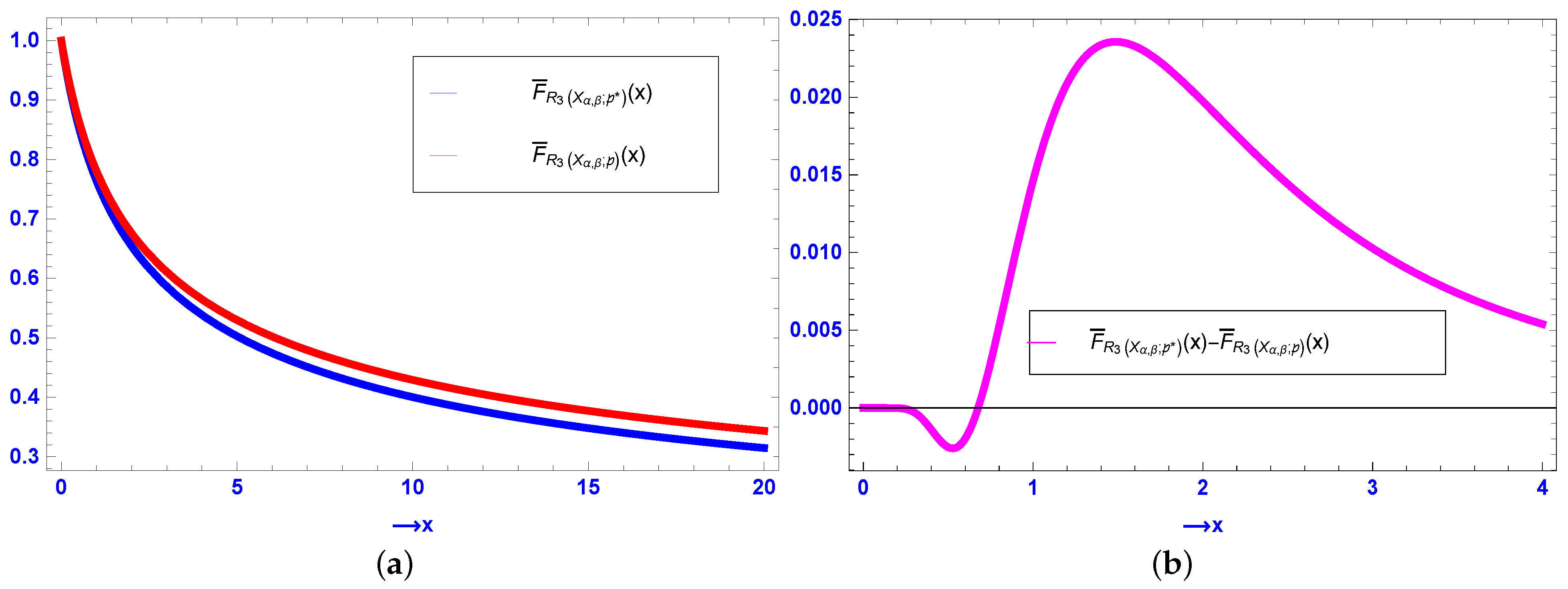
Example 2.

Assume that $\mathit{p}=(0.1,0.3,0.6)$, ${\mathit{p}}^{*}=(0.2,0.3,0.5)$, $\mathit{\beta }=(0.5,0.4,0.3)$, and $\alpha =0.5$. Clearly, the assumptions made in Theorem 2 are satisfied. Using the numerical values, we plot the graphs of $R_3({\mathit{X}}_{\alpha ,\mathit{\beta }};{\mathit{p}}^{*})$ and $R_3({\mathit{X}}_{\alpha ,\mathit{\beta }};\mathit{p})$ in Figure 2a, validating the usual stochastic order in Theorem 2.

Figure 2. (a) Plots of the sfs of $R_3({\mathit{X}}_{\alpha ,\mathit{\beta }};{\mathit{p}}^{*})$ (purple curve) and $R_3({\mathit{X}}_{\alpha ,\mathit{\beta }};\mathit{p})$ (orange curve) in Example 2. (b) Plots of the sfs of $R_3({\mathit{X}}_{{\mathit{\alpha }}^{*},\beta };\mathit{p})$ (green curve) and $R_3({\mathit{X}}_{\mathit{\alpha },\beta };\mathit{p})$ (pink curve) in Example 3.

Next, we consider a counterexample to establish that the result in Theorem 2 does not hold if $(\mathit{\beta },\mathit{p})$ and $(\mathit{\beta },{\mathit{p}}^{*})$ do not belong to ${\mathcal{L}}_3$.

Counterexample 2.

For $n=3$, set $\mathit{p}=(0.2,0.6,0.2)$, ${\mathit{p}}^{*}=(0.2,0.5,0.3)$, $\mathit{\beta }=(5.2,15.8,5.6)$, and $\alpha =1$. Here, though ${\mathit{p}}^{*}\stackrel{w}{\preccurlyeq }\mathit{p}$ holds, the conditions $(\mathit{\beta },\mathit{p})\in {\mathcal{L}}_3$ and $(\mathit{\beta },{\mathit{p}}^{*})\in {\mathcal{L}}_3$ do not hold. Write

$$\begin{array}{ccc}\hfill K_1\left(x\right)& =& {\overline{F}}_{R_3({\mathit{X}}_{\alpha ,\mathit{\beta }};{\mathit{p}}^{*})}\left(x\right)-{\overline{F}}_{R_3({\mathit{X}}_{\alpha ,\mathit{\beta }};\mathit{p})}\left(x\right)\hfill \\ & =& \sum _{i=1}^3{p}_i^{*}[1-{(1-{(1+x)}^{-1})}^{{\beta }_i}]-\sum _{i=1}^3{p}_i[1-{(1-{(1+x)}^{-1})}^{{\beta }_i}].\hfill \end{array}$$

(5)

Now, for $x=10$, $K_1\left(10\right)=0.00262105(>0)$ and for $x=100$, $K_1\left(100\right)=-0.00408561(<0)$, establishing that $K_1\left(x\right)$ changes its sign. Thus, clearly the usual stochastic order between $R_3({\mathit{X}}_{\alpha ,\mathit{\beta }};{\mathit{p}}^{*})$ and $R_3({\mathit{X}}_{\alpha ,\mathit{\beta }};\mathit{p})$ does not hold.

In the upcoming theorem, we consider heterogeneity in the shape parameter $\alpha$, while $\beta$ is fixed. In addition, we assume the mixing proportion vector $\mathit{p}$ to be common. Denote ${\mathit{X}}_{{\mathit{\alpha }}^{*},\beta }=(X_{{\alpha }_1^{*},\beta },\dots ,X_{{\alpha }_n^{*},\beta })$.

Theorem 3.

Under the setup as in Assumption 1, with ${\beta }_1=\dots ={\beta }_n=\beta (0<\beta <1)$, for $(\mathit{\alpha },\mathit{p}),({\mathit{\alpha }}^{*},\mathit{p})\in {\mathcal{L}}_n$, we have

$$\begin{array}{c}\hfill {\mathit{\alpha }}^{*}\stackrel{w}{\preccurlyeq }\mathit{\alpha }\Rightarrow R_n({\mathit{X}}_{{\mathit{\alpha }}^{*},\beta };\mathit{p}){\le }_{st}{R}_n({\mathit{X}}_{\mathit{\alpha },\beta };\mathit{p}).\end{array}$$

Proof. 

See Appendix A. □

The following example illustrates Theorem 3.

Example 3.

Consider $n=3$, $\mathit{\alpha }=(1.1,0.9,0.4)$, ${\mathit{\alpha }}^{*}=(1.2,0.9,0.8)$, $\mathit{p}=(0.1,0.2,0.7)$, and $\beta =0.5$. Clearly, the assumptions made in Theorem 3 are satisfied. Using the numerical values, we plot the graphs of ${\overline{F}}_{R_3({\mathit{X}}_{{\mathit{\alpha }}^{*},\beta };\mathit{p})}\left(x\right)$ and ${\overline{F}}_{R_3({\mathit{X}}_{\mathit{\alpha },\beta };\mathit{p})}\left(x\right)$ in Figure 2b, validating the usual stochastic order in Theorem 3.

Next, we present a counterexample to show that the condition ${\mathit{\alpha }}^{*}\stackrel{w}{\preccurlyeq }\mathit{\alpha }$ in Theorem 3 cannot be dropped to get the usual stochastic ordering between the MRVs.

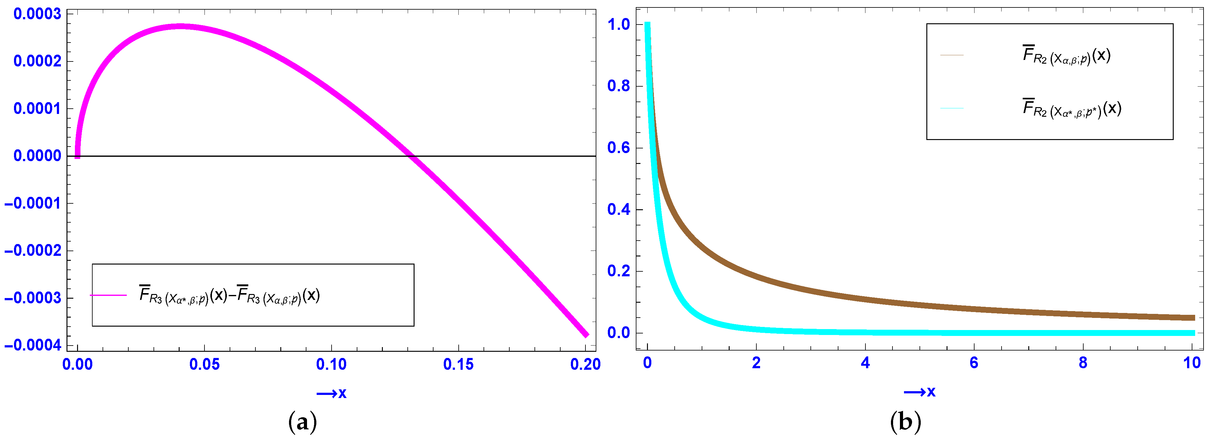
Counterexample 3.

Assume that $n=3$, $\mathit{\alpha }=(1.2,0.8,0.7)$, ${\mathit{\alpha }}^{*}=(1.5,0.9,0.55)$, $\mathit{p}=(0.20,0.35,0.45)$, and $\beta =0.5$. Here, $(1.5,0.9,0.55)\stackrel{w}{⋠}(1.2,0.8,0.7)$, while other conditions are satisfied. We plot the difference ${\overline{F}}_{R_3({\mathit{X}}_{{\mathit{\alpha }}^{*},\beta };\mathit{p})}\left(x\right)-{\overline{F}}_{R_3({\mathit{X}}_{\mathit{\alpha },\beta };\mathit{p})}\left(x\right)$ in Figure 3a, which suggests that the usual stochastic order between $R_3({\mathit{X}}_{{\mathit{\alpha }}^{*},\beta };\mathit{p})$ and $R_3({\mathit{X}}_{\mathit{\alpha },\beta };\mathit{p})$ does not hold.

Figure 3. (a) Plot of the difference between the sfs of $R_3({\mathit{X}}_{{\mathit{\alpha }}^{*},\beta };\mathit{p})$ and $R_3({\mathit{X}}_{\mathit{\alpha },\beta };\mathit{p})$ in Counterexample 3. (b) Plots of the sfs of $R_2({\mathit{X}}_{\mathit{\alpha },\beta };\mathit{p})$ (brown curve) and $R_2({\mathit{X}}_{{\mathit{\alpha }}^{*},\beta };{\mathit{p}}^{*})$ (cyan curve) in Example 4.

3.2. Ordering Results for MMs When Heterogeneity Presents in Two Parameters

In the previous subsection, we have assumed heterogeneity in one parameter. There are various situations where more than one parameter is heterogeneous. In this subsection, we consider heterogeneity in two parameters and obtain some ordering results. The results are established using the concept of chain majorization between the parameter-matrices of two MMs. The following lemma is useful in proving the upcoming theorem.

Lemma 3.

The function $\zeta (x;\alpha ,\beta )={(1+x)}^{-\alpha }{(1-{(1+x)}^{-\alpha })}^{\beta -1}$, for fixed $x>0$ and $0<\beta <1$, is decreasing with respect to $\alpha >0$.

Proof. 

The proof is straightforward, and thus, it is omitted. □

Theorem 4.

Let ${\overline{F}}_{R_2({\mathit{X}}_{\mathit{\alpha },\beta };\mathit{p})}\left(x\right)={\sum }_{i=1}^2{p}_i[1-{(1-{(1+x)}^{-{\alpha }_i})}^{\beta }]$ and ${\overline{F}}_{R_2({\mathit{X}}_{{\mathit{\alpha }}^{*},\beta };{\mathit{p}}^{*})}\left(x\right)={\sum }_{i=1}^2{p}_i^{*}[1-{(1-{(1+x)}^{-{\alpha }_i^{*}})}^{\beta }]$ be the sfs of the MRVs $R_2({\mathit{X}}_{\mathit{\alpha },\beta };\mathit{p})$ and $R_2({\mathit{X}}_{{\mathit{\alpha }}^{*},\beta };{\mathit{p}}^{*})$, respectively. For $(\mathit{p},\mathit{\alpha })\in {\mathcal{L}}_2$ and $\beta \in (0,1)$, we have

$$\left[\begin{array}{cc}{p}_1& p_2\\ {\alpha }_1& {\alpha }_2\end{array}\right]\gg \left[\begin{array}{cc}{p}_1^{*}& p_2^{*}\\ {\alpha }_1^{*}& {\alpha }_2^{*}\end{array}\right]\Rightarrow R_2({\mathit{X}}_{\mathit{\alpha },\beta };\mathit{p}){\ge }_{st}{R}_2({\mathit{X}}_{{\mathit{\alpha }}^{*},\beta };{\mathit{p}}^{*}).$$

Proof. 

See Appendix A. □

To validate Theorem 4, we consider the following example.

Example 4.

For $n=2$, consider $\mathit{p}=(0.6,0.4)$, ${\mathit{p}}^{*}=(0.46,0.54)$, $\mathit{\alpha }=(1,9)$, $\mathit{\lambda }=(6.6,3.4)$, and $\beta =0.5$. Clearly, we observe that $\left(\begin{array}{cc}0.6& 0.4\\ 1& 9\end{array}\right)\in {\mathcal{L}}_2$. Take a T-transform matrix $T_{0.3}=\left(\begin{array}{cc}0.3& 0.7\\ 0.7& 0.3\end{array}\right)$. It can then be seen that

$$\left(\begin{array}{cc}0.46& 0.54\\ 6.6& 3.4\end{array}\right)=\left(\begin{array}{cc}0.6& 0.4\\ 1& 9\end{array}\right)\times \left(\begin{array}{cc}0.3& 0.7\\ 0.7& 0.3\end{array}\right).$$

Thus,

$$\left(\begin{array}{cc}0.6& 0.4\\ 1& 9\end{array}\right)\gg \left(\begin{array}{cc}0.46& 0.54\\ 6.6& 3.4\end{array}\right),$$

and from Theorem 4, we obtain $R_2({\mathit{X}}_{\mathit{\alpha },\beta };\mathit{p}){\ge }_{st}{R}_2({\mathit{X}}_{{\mathit{\alpha }}^{*},\beta };{\mathit{p}}^{*})$, as observed in Figure 3b.

Note that Theorem 4 has been established for $\beta \in (0,1)$ with other sufficient conditions. Thus, one may be curious to know whether the usual stochastic order in Theorem 4 holds if $\beta$ is not in $(0,1)$. In this regard, we consider the next counterexample.

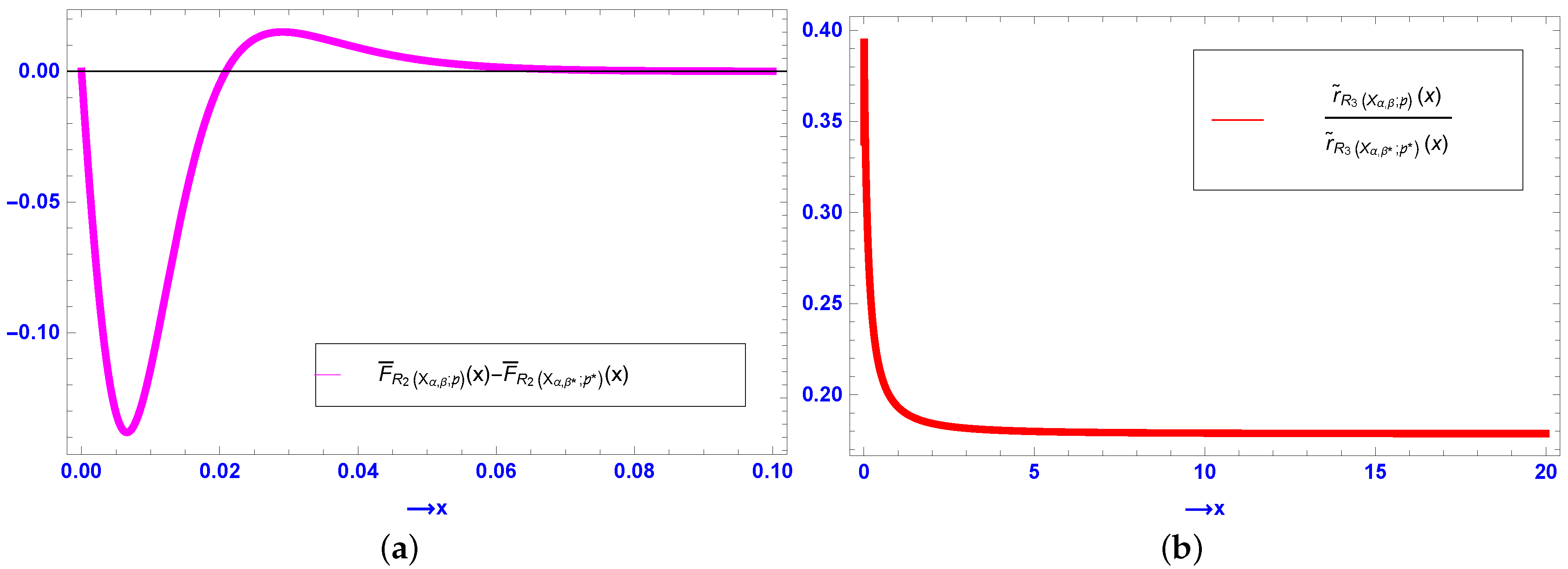
Counterexample 4.

For $n=2$, set $\mathit{\alpha }=(2,3)$, $\mathit{p}=(0.7,0.3)$, ${\mathit{\alpha }}^{*}=(2.6,2.4)$, ${\mathit{p}}^{*}=(0.46,0.54)$, and $\beta =100$. Clearly, $\beta \notin (0,1)$. Further, for a T-transform matrix $T_{0.4}=\left(\begin{array}{cc}0.4& 0.6\\ 0.6& 0.4\end{array}\right)$, we obtain

$$\left(\begin{array}{cc}0.46& 0.54\\ 2.6& 2.4\end{array}\right)=\left(\begin{array}{cc}0.7& 0.3\\ 2& 3\end{array}\right)\times \left(\begin{array}{cc}0.4& 0.6\\ 0.6& 0.4\end{array}\right),$$

implying that

$$\left(\begin{array}{cc}0.7& 0.3\\ 2& 3\end{array}\right)\gg \left(\begin{array}{cc}0.46& 0.54\\ 2.6& 2.4\end{array}\right).$$

Now, we plot the graph of the difference of the sfs of $R_2({\mathit{X}}_{\mathit{\alpha },\beta };\mathit{p})$ and $R_2({\mathit{X}}_{{\mathit{\alpha }}^{*},\beta };{\mathit{p}}^{*})$ in Figure 4a. From this figure, the usual stochastic order between $R_2({\mathit{X}}_{\mathit{\alpha },\beta };\mathit{p})$ and $R_2({\mathit{X}}_{{\mathit{\alpha }}^{*},\beta };{\mathit{p}}^{*})$ does not hold, since the graph crosses the x-axis.

Figure 4. (a) Plot of the difference between the sfs of $R_2({\mathit{X}}_{\mathit{\alpha },\beta };\mathit{p})$ and $R_2({\mathit{X}}_{{\mathit{\alpha }}^{*},\beta };{\mathit{p}}^{*})$ in Counterexample 4. (b) Plots of the sfs of $R_2({\mathit{X}}_{\alpha ,\mathit{\beta }};\mathit{p})$ (purple curve) and $R_2({\mathit{X}}_{\alpha ,{\mathit{\beta }}^{*}};{\mathit{p}}^{*})$ (black curve) in Example 5.

Next, we extend the result in Theorem 4 for n number of subpopulations.

Theorem 5.

Let ${\overline{F}}_{R_n({\mathit{X}}_{\mathit{\alpha },\beta };\mathit{p})}\left(x\right)={\sum }_{i=1}^n{p}_i[1-{(1-{(1+x)}^{-{\alpha }_i})}^{\beta }]$ and ${\overline{F}}_{R_n({\mathit{X}}_{{\mathit{\alpha }}^{*},\beta };{\mathit{p}}^{*})}\left(x\right)={\sum }_{i=1}^n{p}_i^{*}[1-{(1-{(1+x)}^{-{\alpha }_i^{*}})}^{\beta }]$ be the sfs of the MRVs $R_n({\mathit{X}}_{\mathit{\alpha },\beta };\mathit{p})$ and $R_n({\mathit{X}}_{{\mathit{\alpha }}^{*},\beta };{\mathit{p}}^{*})$, respectively. For $(\mathit{p},\mathit{\alpha })\in {\mathcal{L}}_n$ and $\beta \in (0,1)$,

$$\left(\begin{array}{c}{p}_1\dots p_n\\ {\alpha }_1\dots {\alpha }_n\end{array}\right)\gg \left(\begin{array}{c}{p}_1^{*}\dots p_n^{*}\\ {\alpha }_1^{*}\dots {\alpha }_n^{*}\end{array}\right)\Rightarrow R_n({\mathit{X}}_{\mathit{\alpha },\beta };\mathit{p}){\ge }_{st}{R}_n({\mathit{X}}_{{\mathit{\alpha }}^{*},\beta };{\mathit{p}}^{*}).$$

Proof. 

The proof of this theorem is similar to that of Theorem $4.2$ of [17]. Thus, it is omitted. □

It is well-known fact that a finite product of T-transform matrices with a common structure yields a T-transform matrix. Using this, the following corollary is an immediate consequence of Theorem 5.

Corollary 2.

Consider k number of T-transformed matrices with a common structure, denoted by $T_{{\omega }_1},\dots ,T_{{\omega }_n}$. Then, under the setup in Theorem 5, with $(\mathit{p},\mathit{\alpha })\in {\mathcal{L}}_n$ and $\beta \in (0,1)$,

$$\left(\begin{array}{c}{p}_1\dots p_n\\ {\alpha }_1\dots {\alpha }_n\end{array}\right)\gg \left(\begin{array}{c}{p}_1^{*}\dots p_n^{*}\\ {\alpha }_1^{*}\dots {\alpha }_n^{*}\end{array}\right)\Rightarrow R_n({\mathit{X}}_{\mathit{\alpha },\beta };\mathit{p}){\ge }_{st}{R}_n({\mathit{X}}_{{\mathit{\alpha }}^{*},\beta };{\mathit{p}}^{*}).$$

From the result in Corollary 2, an obvious question is “does the result in Corollary 2 hold if the T-transform matrices have different structures?” In the next theorem we discuss this issue. We observe that a similar result to Corollary 2 holds with an additional assumption.

Theorem 6.

Consider k number of T-transformed matrices with different structures, denoted by $T_{{\omega }_1},\dots ,T_{{\omega }_k}$. Then, under the similar setup as in Theorem 5, with $(\mathit{p},\mathit{\alpha })\in {\mathcal{L}}_n$, $(\mathit{p},\mathit{\alpha })T_{{\omega }_1}\dots T_{{\omega }_i}\in {\mathcal{L}}_n$, $i=1,\dots ,k-1,(k\ge 2)$, and $\beta \in (0,1)$,

$$\left(\begin{array}{c}{p}_1^{*}\dots p_n^{*}\\ {\alpha }_1^{*}\dots {\alpha }_n^{*}\end{array}\right)=\left(\begin{array}{c}{p}_1\dots p_n\\ {\alpha }_1\dots {\alpha }_n\end{array}\right)T_{{\omega }_1}\dots T_{{\omega }_k}\Rightarrow R_n({\mathit{X}}_{\mathit{\alpha },\beta };\mathit{p}){\ge }_{st}{R}_n({\mathit{X}}_{{\mathit{\alpha }}^{*},\beta };{\mathit{p}}^{*}).$$

Proof. 

The proof is similar to that of the proof of Theorem $4.3$ of [17]. Hence, it is not presented. □

The preceding results of this subsection deal with the stochastic comparison of two MRVs when the matrix $(\mathit{p},\mathit{\alpha })$ changes to another matrix $({\mathit{p}}^{*},{\mathit{\alpha }}^{*})$ with fixed $\beta$. In the upcoming results, we assume that the matrix $(\mathit{p},\mathit{\beta })$ changes to $({\mathit{p}}^{*},{\mathit{\beta }}^{*})$ with fixed $\alpha$. First, we consider two subpopulations. The following lemma is useful to establish the next theorem.

Lemma 4.

The function $\varkappa (x;p,\alpha ,\beta )=p{(1-{(1+x)}^{-\alpha })}^{\beta }$

(i)

is decreasing with respect to β for fixed $p>0$, $\alpha >0$;

(ii)

is increasing with respect to p for fixed $\beta >0$, $\alpha >0$.

Proof. 

The proof is straightforward, and thus, it is omitted. □

Theorem 7.

Let ${\overline{F}}_{R_2({\mathit{X}}_{\alpha ,\mathit{\beta }};\mathit{p})}\left(x\right)={\sum }_{i=1}^2{p}_i[1-{(1-{(1+x)}^{-\alpha })}^{{\beta }_i}]$ and ${\overline{F}}_{R_2({\mathit{X}}_{\alpha ,{\mathit{\beta }}^{*}};{\mathit{p}}^{*})}\left(x\right)={\sum }_{i=1}^2{p}_i^{*}[1-{(1-{(1+x)}^{-\alpha })}^{{\beta }_i^{*}}]$ be the sfs of the MRVs $R_n({\mathit{X}}_{\alpha ,\mathit{\beta }};\mathit{p})$ and $R_n({\mathit{X}}_{\alpha ,{\mathit{\beta }}^{*}};{\mathit{p}}^{*})$, respectively. For $(\mathit{p},\mathit{\beta })\in {\mathcal{L}}_2$ and fixed $\alpha >0$,

$$\left[\begin{array}{cc}{p}_1& p_2\\ {\beta }_1& {\beta }_2\end{array}\right]\gg \left[\begin{array}{cc}{p}_1^{*}& p_2^{*}\\ {\beta }_1^{*}& {\beta }_2^{*}\end{array}\right]\Rightarrow R_2({\mathit{X}}_{\alpha ,\mathit{\beta }};\mathit{p}){\le }_{st}{R}_2({\mathit{X}}_{\alpha ,{\mathit{\beta }}^{*}};{\mathit{p}}^{*}).$$

Proof. 

See Appendix A. □

In order to justify Theorem 7, an example is provided.

Example 5.

Let $\mathit{p}=(0.2,0.8)$, ${\mathit{p}}^{*}=(0.74,0.26)$, $\mathit{\beta }=(6,2)$, ${\mathit{\beta }}^{*}=(2.4,5.6)$, and $\alpha =0.6$. It is not hard to check that $(\mathit{p},\mathit{\beta })\in {\mathcal{L}}_2$. Further, let $T_{0.1}=\left(\begin{array}{cc}0.1& 0.9\\ 0.9& 0.1\end{array}\right)$. It can then be seen that

$$\left(\begin{array}{cc}0.74& 0.26\\ 2.4& 5.6\end{array}\right)=\left(\begin{array}{cc}0.2& 0.8\\ 6& 2\end{array}\right)\times \left(\begin{array}{cc}0.1& 0.9\\ 0.9& 0.1\end{array}\right),$$

which implies that

$$\left(\begin{array}{cc}0.2& 0.8\\ 6& 2\end{array}\right)\gg \left(\begin{array}{cc}0.74& 0.26\\ 2.4& 5.6\end{array}\right).$$

Thus, from Theorem 7, we obtain $R_2({\mathit{X}}_{\alpha ,\mathit{\beta }};\mathit{p}){\le }_{st}{R}_2({\mathit{X}}_{\alpha ,{\mathit{\beta }}^{*}};{\mathit{p}}^{*})$, which can be verified from Figure 4b.

The following counterexample shows that the desired ordering result in Theorem 7 does not hold if $(\mathit{p},\mathit{\beta })\notin {\mathcal{L}}_2$.

Counterexample 5.

Let us assume

$$\left(\begin{array}{cc}{p}_1& p_2\\ {\beta }_1& {\beta }_2\end{array}\right)=\left(\begin{array}{cc}0.6& 0.4\\ 7& 1\end{array}\right)\notin {\mathcal{L}}_{2}and\left(\begin{array}{cc}{p}_1^{*}& p_2^{*}\\ {\beta }_1^{*}& {\beta }_2^{*}\end{array}\right)=\left(\begin{array}{cc}0.48& 0.52\\ 3.4& 4.6\end{array}\right)\notin {\mathcal{L}}_2.$$

It is then easy to check that

$$\left(\begin{array}{cc}0.48& 0.52\\ 3.4& 4.6\end{array}\right)=\left(\begin{array}{cc}0.6& 0.4\\ 7& 1\end{array}\right)\times \left(\begin{array}{cc}0.4& 0.6\\ 0.6& 0.4\end{array}\right),$$

where $T_{0.4}=\left(\begin{array}{cc}0.4& 0.6\\ 0.6& 0.4\end{array}\right)$, implying that

$$\left(\begin{array}{cc}0.6& 0.4\\ 7& 1\end{array}\right)\gg \left(\begin{array}{cc}0.48& 0.52\\ 3.4& 4.6\end{array}\right).$$

Now, the difference between the sfs of the MRVs $R_2({\mathit{X}}_{\alpha ,\mathit{\beta }};\mathit{p})$ and $R_2({\mathit{X}}_{\alpha ,{\mathit{\beta }}^{*}};{\mathit{p}}^{*})$ is plotted in Figure 5a. Clearly, the difference takes negative as well as positive values, which means that the desired usual stochastic order in Theorem 7 does not hold.

Figure 5. (a) Plot of the difference between the sfs of $R_2({\mathit{X}}_{\alpha ,\mathit{\beta }};\mathit{p})$ and $R_2({\mathit{X}}_{\alpha ,{\mathit{\beta }}^{*}};{\mathit{p}}^{*})$ in Counterexample 5. (b) Plot of the ratio of the rhs of $R_3({\mathit{X}}_{\alpha ,\mathit{\beta }};\mathit{p})$ and $R_3({\mathit{X}}_{\alpha ,{\mathit{\beta }}^{*}};{\mathit{p}}^{*})$ in Example 6.

Next, we present a result dealing with n number of subpopulations.

Theorem 8.

Let ${\overline{F}}_{R_n({\mathit{X}}_{\alpha ,\mathit{\beta }};\mathit{p})}\left(x\right)={\sum }_{i=1}^n{p}_i[1-{(1-{(1+x)}^{-\alpha })}^{{\beta }_i}]$ and ${\overline{F}}_{R_n({\mathit{X}}_{\alpha ,{\mathit{\beta }}^{*}};{\mathit{p}}^{*})}\left(x\right)={\sum }_{i=1}^n{p}_i^{*}$$[1-{(1-{(1+x)}^{-\alpha })}^{{\beta }_i^{*}}]$ be the sfs of the MRVs $R_n({\mathit{X}}_{\alpha ,\mathit{\beta }};\mathit{p})$ and $R_n({\mathit{X}}_{\alpha ,{\mathit{\beta }}^{*}};{\mathit{p}}^{*})$, respectively. For $(\mathit{p},\mathit{\beta })\in {\mathcal{L}}_n$ and fixed $\alpha >0$,

$$\left(\begin{array}{c}{p}_1\dots p_n\\ {\beta }_1\dots {\beta }_n\end{array}\right)\gg \left(\begin{array}{c}{p}_1^{*}\dots p_n^{*}\\ {\beta }_1^{*}\dots {\beta }_n^{*}\end{array}\right)\Rightarrow R_n({\mathit{X}}_{\alpha ,\mathit{\beta }};\mathit{p}){\le }_{st}{R}_n({\mathit{X}}_{\alpha ,{\mathit{\beta }}^{*}};{\mathit{p}}^{*}).$$

Proof. 

The proof is similar to that of Theorem 5, and thus, it is omitted. □

The following corollary can be established from Theorem 8 using arguments similar to Corollary 2.

Corollary 3.

Consider k number of T-transform matrices denoted by $T_{{\omega }_1},\dots ,T_{{\omega }_k}$ having a common structure. Then, under the setup in Theorem 8, for $(\mathit{p},\mathit{\beta })\in {\mathcal{L}}_n$ and fixed $\alpha >0$,

$$\left(\begin{array}{c}{p}_1\dots p_n\\ {\beta }_1\dots {\beta }_n\end{array}\right)\gg \left(\begin{array}{c}{p}_1^{*}\dots p_n^{*}\\ {\beta }_1^{*}\dots {\beta }_n^{*}\end{array}\right)\Rightarrow R_n({\mathit{X}}_{\alpha ,\mathit{\beta }};\mathit{p}){\le }_{st}{R}_n({\mathit{X}}_{\alpha ,{\mathit{\beta }}^{*}};{\mathit{p}}^{*}).$$

The next theorem proves a result associated with k$(\ge 2)$ number of T-transformed matrices having different structures.

Theorem 9.

Let $T_{{\omega }_1},\dots ,T_{{\omega }_i}$, $i=1,\dots ,k(k\ge 2)$ be the k number of T-transformed matrices with different structures. Then, under the setup as in Theorem 8, for $(\mathit{p},\mathit{\beta })\in {\mathcal{L}}_n$, $\left(\begin{array}{c}{p}_1\dots p_n\\ {\beta }_1\dots {\beta }_n\end{array}\right)T_{{\omega }_1}\dots T_{{\omega }_i}\in {\mathcal{L}}_n$, $i=1,\dots ,(k-1)$, and fixed $\alpha >0$,

$$\left(\begin{array}{c}{p}_1^{*}\dots p_n^{*}\\ {\beta }_1^{*}\dots {\beta }_n^{*}\end{array}\right)=\left(\begin{array}{c}{p}_1\dots p_n\\ {\beta }_1\dots {\beta }_n\end{array}\right)T_{{\omega }_1}\dots T_{{\omega }_k}\Rightarrow R_n({\mathit{X}}_{\alpha ,\mathit{\beta }};\mathit{p}){\le }_{st}{R}_n({\mathit{X}}_{\alpha ,{\mathit{\beta }}^{*}};{\mathit{p}}^{*}).$$

We end this subsection with ageing faster order between two MRVs. Here, we assume that the mixing proportions and one of the shape parameter vectors are varying. We recall that using ageing faster order one is able to compare the relative ageings of two engineering systems. In the following theorem, we study the ageing faster order in terms of the reversed hazard rate function.

Theorem 10.

Let $R_n({\mathit{X}}_{\alpha ,\mathit{\beta }};\mathit{p})$ and $R_n({\mathit{X}}_{\alpha ,{\mathit{\beta }}^{*}};{\mathit{p}}^{*})$ be the MRVs with reversed hazard functions ${\tilde{r}}_{R_n({\mathit{X}}_{\alpha ,\mathit{\beta }};\mathit{p})}\left(x\right)$ and ${\tilde{r}}_{R_n({\mathit{X}}_{\alpha ,{\mathit{\beta }}^{*}};{\mathit{p}}^{*})}\left(x\right)$, respectively. Then,

$$\begin{array}{c}\hfill R_n({\mathit{X}}_{\alpha ,\mathit{\beta }};\mathit{p}){\le }_{R-rh}{R}_n({\mathit{X}}_{\alpha ,{\mathit{\beta }}^{*}};{\mathit{p}}^{*}),\end{array}$$

provided $\underset{\{i,j:i\ne j\}}{max}|{\beta }_i-{\beta }_j|\le \underset{\{i,j:i\ne j\}}{min}|{\beta }_i^{*}-{\beta }_j^{*}|$, for all $i,j=1,\dots ,n$.

Proof. 

See Appendix A. □

The following example illustrates Theorem 10 for $n=3$.

Example 6.

Assume that $\mathit{\beta }=(0.1,0.2,0.3)$, ${\mathit{\beta }}^{*}=(0.5,1,2)$, $\mathit{p}=(0.1,0.3,0.6)$, ${\mathit{p}}^{*}=(0.2,0.3,0.5)$, and $\alpha =2$. Clearly, the condition $max|{\beta }_i-{\beta }_j|\le min|{\beta }_i^{*}-{\beta }_j^{*}|$ is satisfied for $i\ne j=1,2,3$. Taking these numerical values of the parameters, ${\tilde{r}}_{R_3({\mathit{X}}_{\alpha ,\mathit{\beta }};\mathit{p})}\left(x\right)/{\tilde{r}}_{R_3({\mathit{X}}_{\alpha ,{\mathit{\beta }}^{*}};{\mathit{p}}^{*})}\left(x\right)$ is plotted in Figure 5b, validating the result in Theorem 10.

3.3. Ordering Results for MMs When Heterogeneity Presents in Three Parameters

In the previous subsection, we assume that two parameters are heterogeneous. In this subsection, we present the ordering results considering heterogeneity in three parameters. We mainly obtain the stochastic comparison results between two MRVs with respect to the reversed hazard rate and likelihood ratio orders. First, we provide the reversed hazard rate order between $R_n({\mathit{X}}_{\mathit{\alpha },\mathit{\beta }};\mathit{p})$ and $R_n({\mathit{X}}_{{\mathit{\alpha }}^{*},{\mathit{\beta }}^{*}};{\mathit{p}}^{*})$.

Theorem 11.

Consider two MRVs $R_n({\mathit{X}}_{\mathit{\alpha },\mathit{\beta }};\mathit{p})$ and $R_n({\mathit{X}}_{{\mathit{\alpha }}^{*},{\mathit{\beta }}^{*}};{\mathit{p}}^{*})$ with sfs ${\overline{F}}_{R_n({\mathit{X}}_{\mathit{\alpha },\mathit{\beta }};\mathit{p})}\left(x\right)$ and ${\overline{F}}_{R_n({\mathit{X}}_{{\mathit{\alpha }}^{*},{\mathit{\beta }}^{*}};{\mathit{p}}^{*})}\left(x\right)$, respectively. Then,

$$\begin{array}{c}\hfill R_n({\mathit{X}}_{\mathit{\alpha },\mathit{\beta }};\mathit{p}){\le }_{rh}{R}_n({\mathit{X}}_{{\mathit{\alpha }}^{*},{\mathit{\beta }}^{*}};{\mathit{p}}^{*}),\end{array}$$

provided $max\{{\alpha }_1^{*},\dots ,{\alpha }_n^{*}\}\le min\{{\alpha }_1,\dots ,{\alpha }_n\}$ and $max\{{\alpha }_1{\beta }_1,\dots ,{\alpha }_n{\beta }_n\}\le min\{{\alpha }_1^{*}{\beta }_1^{*},\dots ,{\alpha }_n^{*}{\beta }_n^{*}\}$.

Proof. 

See Appendix A. □

An illustrative example is provided below for $n=3$.

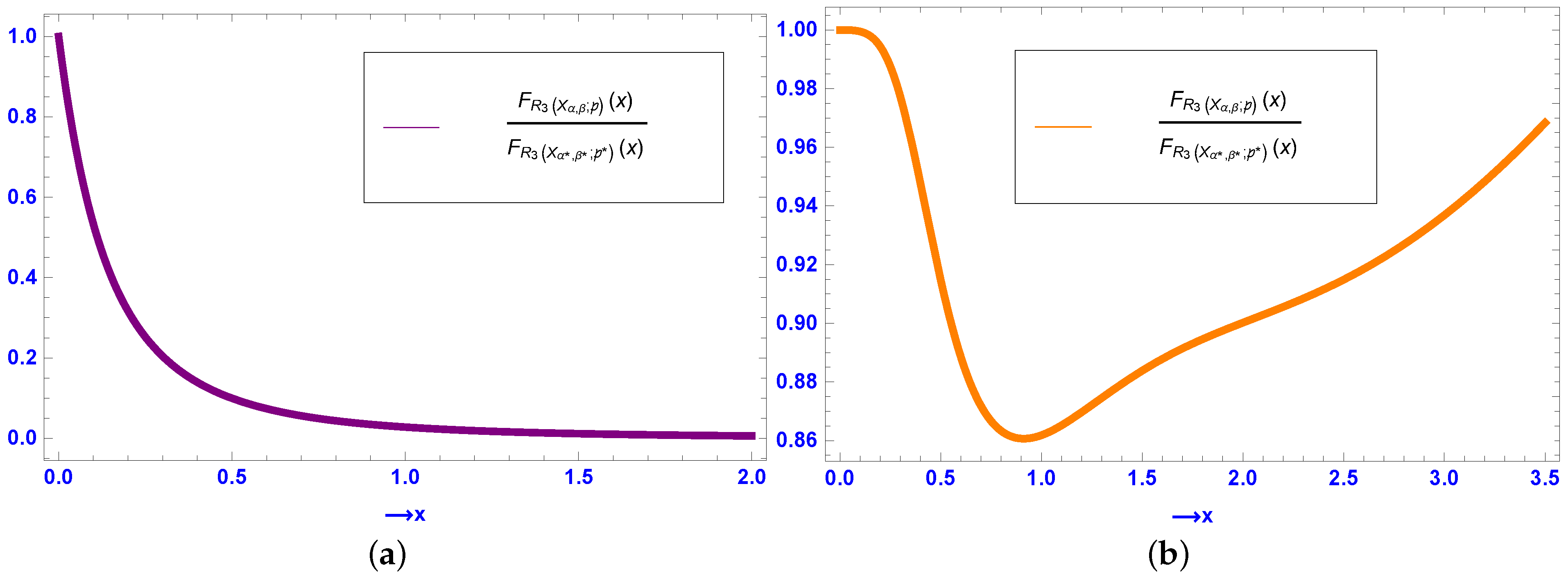
Example 7.

Assume that $\mathit{p}=(0.1,0.7,0.2)$, ${\mathit{p}}^{*}=(0.2,0.5,0.3)$, $\mathit{\alpha }=(5,8,6)$, $\mathit{\beta }=(2,1,1)$, ${\mathit{\alpha }}^{*}=(3,4,2)$, and ${\mathit{\beta }}^{*}=(5,3,6)$. Clearly, $max\{3,4,2\}\le min\{5,8,6\}$ and $max\{10,8,6\}\le min\{15,12,12\}$. Thus, the conditions of Theorem 11 hold. Now, the ratio of the cdfs of $R_3({\mathit{X}}_{\mathit{\alpha },\mathit{\beta }};\mathit{p})$ and $R_3({\mathit{X}}_{{\mathit{\alpha }}^{*},{\mathit{\beta }}^{*}};{\mathit{p}}^{*})$ is plotted in Figure 6a, illustrating the result $R_3({\mathit{X}}_{\mathit{\alpha },\mathit{\beta }};\mathit{p}){\le }_{rh}{R}_3({\mathit{X}}_{{\mathit{\alpha }}^{*},{\mathit{\beta }}^{*}};{\mathit{p}}^{*})$ in Theorem 11.

Figure 6. (a) Plot of the ratio of the cdfs of $R_3({\mathit{X}}_{\mathit{\alpha },\mathit{\beta }};\mathit{p})$ and $R_3({\mathit{X}}_{{\mathit{\alpha }}^{*},{\mathit{\beta }}^{*}};{\mathit{p}}^{*})$ in Example 7. (b) Plot of the ratio of the cdfs of $R_3({\mathit{X}}_{\mathit{\alpha },\mathit{\beta }};\mathit{p})$ and $R_3({\mathit{X}}_{{\mathit{\alpha }}^{*},{\mathit{\beta }}^{*}};{\mathit{p}}^{*})$ in Counterexample 6.

The following counterexample illustrates that the result in Theorem 11 does not hold if $max\{{\alpha }_1^{*},{\alpha }_2^{*},{\alpha }_3^{*}\}\nleqq min\{{\alpha }_1,{\alpha }_2,{\alpha }_3\}$.

Counterexample 6.

Set $\mathit{p}=(0.60,0.25,0.15)$, ${\mathit{p}}^{*}=(0.45,0.30,0.25)$, $\mathit{\alpha }=(1,3,5)$, $\mathit{\beta }=(3,6,9)$, ${\mathit{\alpha }}^{*}=(2,4,6)$, and ${\mathit{\beta }}^{*}=(25,30,35)$. Obviously, $max\{2,4,6\}\nleqq min\{1,3,5\}$ and $max\{3,18,45\}\le min\{50,120,210\}$. It can be seen that all the conditions of Theorem 11 are satisfied except $max\{2,4,6\}\le min\{1,3,5\}$. Now, the ratio of the cdfs of the MRVs $R_3({\mathit{X}}_{\mathit{\alpha },\mathit{\beta }};\mathit{p})$ and $R_3({\mathit{X}}_{{\mathit{\alpha }}^{*},{\mathit{\beta }}^{*}};{\mathit{p}}^{*})$ is presented in Figure 6b, from which we see that the ratio is nonmonotone in $x>0$. As a conclusion, $R_3({\mathit{X}}_{\mathit{\alpha },\mathit{\beta }};\mathit{p}){\nleqq }_{rh}{R}_3({\mathit{X}}_{{\mathit{\alpha }}^{*},{\mathit{\beta }}^{*}};{\mathit{p}}^{*})$. In other words, the reversed hazard rate order between $R_3({\mathit{X}}_{\mathit{\alpha },\mathit{\beta }};\mathit{p})$ and $R_3({\mathit{X}}_{{\mathit{\alpha }}^{*},{\mathit{\beta }}^{*}};{\mathit{p}}^{*})$ does not hold.

In the next theorem, under some certain parameter restrictions, the likelihood ratio ordering between two MRVs $R_n({\mathit{X}}_{\mathit{\alpha },\mathit{\beta }};\mathit{p})$ and $R_n({\mathit{X}}_{{\mathit{\alpha }}^{*},{\mathit{\beta }}^{*}};{\mathit{p}}^{*})$ is presented.

Theorem 12.

Let $f_{R_n({\mathit{X}}_{\mathit{\alpha },\mathit{\beta }};\mathit{p})}\left(x\right)={\sum }_{i=1}^n{p}_i{\alpha }_i{\beta }_i{(1+x)}^{-({\alpha }_i+1)}{(1-{(1+x)}^{-{\alpha }_i})}^{{\beta }_i-1}$ and $f_{R_n({\mathit{X}}_{{\mathit{\alpha }}^{*},{\mathit{\beta }}^{*}};{\mathit{p}}^{*})}\left(x\right)$$={\sum }_{i=1}^n{p}_i^{*}{\alpha }_i^{*}{\beta }_i^{*}{(1+x)}^{-({\alpha }_i^{*}+1)}{(1-{(1+x)}^{-{\alpha }_i^{*}})}^{{\beta }_i^{*}-1}$ be the pdfs of the MRVs $R_n({\mathit{X}}_{\mathit{\alpha },\mathit{\beta }};\mathit{p})$ and $R_n({\mathit{X}}_{{\mathit{\alpha }}^{*},{\mathit{\beta }}^{*}};{\mathit{p}}^{*})$, respectively. Then,

$$\begin{array}{c}\hfill R_n({\mathit{X}}_{\mathit{\alpha },\mathit{\beta }};\mathit{p}){\ge }_{lr}{R}_n({\mathit{X}}_{{\mathit{\alpha }}^{*},{\mathit{\beta }}^{*}};{\mathit{p}}^{*}),\end{array}$$

provided $max\{{\alpha }_1,\dots ,{\alpha }_n\}\le min\{{\alpha }_1^{*},\dots ,{\alpha }_n^{*}\}$ and $min\{{\alpha }_1{\beta }_1,\dots ,{\alpha }_n{\beta }_n\}\ge max\{{\alpha }_1^{*}{\beta }_1^{*},\dots ,{\alpha }_n^{*}{\beta }_n^{*}\}$.

Proof. 

See Appendix A. □

The following example illustrates Theorem 12 for $n=3$.

Example 8.

Set $\mathit{p}=(0.2,0.4,0.4)$, ${\mathit{p}}^{*}=(0.3,0.5,0.2)$, $\mathit{\alpha }=(2,4,6)$, $\mathit{\beta }=(25,13,9)$, ${\mathit{\alpha }}^{*}=(8,10,12)$, and ${\mathit{\beta }}^{*}=(3,4,1)$. Observe that $max\{2,4,6\}\le min\{8,10,12\}$ and $max\{24,40,12\}\le min\{50,52,54\}$. Thus, all the conditions of Theorem 12 are satisfied. Based on the numerical values of the parameters, the ratio of the pdfs of the MRVs $R_3({\mathit{X}}_{\mathit{\alpha },\mathit{\beta }};\mathit{p})$ and $R_3({\mathit{X}}_{{\mathit{\alpha }}^{*},{\mathit{\beta }}^{*}};{\mathit{p}}^{*})$ is provided in Figure 7a, which readily establishes that $R_3({\mathit{X}}_{\mathit{\alpha },\mathit{\beta }};\mathit{p}){\ge }_{lr}{R}_3({\mathit{X}}_{{\mathit{\alpha }}^{*},{\mathit{\beta }}^{*}};{\mathit{p}}^{*})$, validating the result in Theorem 12.

Figure 7. (a) Plot of the ratio of the pdfs of $R_3({\mathit{X}}_{\mathit{\alpha },\mathit{\beta }};\mathit{p})$ and $R_3({\mathit{X}}_{{\mathit{\alpha }}^{*},{\mathit{\beta }}^{*}};{\mathit{p}}^{*})$ in Example 8. (b) Plot of the ratio of the pdfs of $R_3({\mathit{X}}_{\mathit{\alpha },\mathit{\beta }};\mathit{p})$ and $R_3({\mathit{X}}_{{\mathit{\alpha }}^{*},{\mathit{\beta }}^{*}};{\mathit{p}}^{*})$ in Counterexample 7.

Next, we present a counterexample to show that the condition $max\{{\alpha }_1,\dots ,{\alpha }_n\}\le min\{{\alpha }_1^{*},\dots ,{\alpha }_n^{*}\}$ is necessary for establishing the likelihood ratio order in Theorem 12.

Counterexample 7.

Let $\mathit{p}=(0.1,0.2,0.7)$, ${\mathit{p}}^{*}=(0.6,0.3,0.1)$, $\mathit{\alpha }=(3,6,9)$, $\mathit{\beta }=(14,15,11)$, ${\mathit{\alpha }}^{*}=(5,8,12)$, and ${\mathit{\beta }}^{*}=(4,2,3)$. Clearly, $max\{3,6,9\}\nleqq min\{5,8,12\}$ and $max\{20,16,36\}\le min\{42,90,99\}$. Thus, all the conditions of Theorem 12 are satisfied except $max\{3,6,9\}\le min\{5,8,12\}$. Now, the ratio of the pdfs of the MRVs $R_3({\mathit{X}}_{\mathit{\alpha },\mathit{\beta }};\mathit{p})$ and $R_3({\mathit{X}}_{{\mathit{\alpha }}^{*},{\mathit{\beta }}^{*}};{\mathit{p}}^{*})$ is depicted in Figure 7b, and we see that the ratio is a nonmonotone function in $x>0$. Thus, $R_3({\mathit{X}}_{\mathit{\alpha },\mathit{\beta }};\mathit{p}){\ngeqq }_{lr}{R}_3({\mathit{X}}_{{\mathit{\alpha }}^{*},{\mathit{\beta }}^{*}};{\mathit{p}}^{*})$. In other words, the likelihood ratio order between $R_3({\mathit{X}}_{\mathit{\alpha },\mathit{\beta }};\mathit{p})$ and $R_3({\mathit{X}}_{{\mathit{\alpha }}^{*},{\mathit{\beta }}^{*}};{\mathit{p}}^{*})$ in Theorem 12 does not hold.

4. Concluding Remarks

In this paper, MMs are considered as suitable tools for analyzing population heterogeneity. We are interested in heterogeneous populations with distinct components such as lifetime. We have derived some sufficient conditions for the comparison between two FMMs of $\mathcal{IK}$ distributed components with respect to the usual stochastic order, reversed hazard rate order, likelihood ratio order, and ageing faster order in terms of reversed hazard rate order, corresponding to the heterogeneity in the model parameters in the sense of some majorization orders, namely, weakly supermajorized and weakly submajorized order. Here, we have considered heterogeneity in one parameter, two parameters, and three parameters. We have presented some numerical examples and counterexamples to illustrate the established results in this paper.

The presented results of this paper are mostly theoretical. However, one may find some applications of the established results. Below, we consider an example.

Assume two engineering systems, with components produced by different companies. It is further reasonable to assume that the components have different reliability characteristics. Each of the components can operate in n operational regimes with corresponding different probabilities $p_i$ and $p_i^{*}$. Let the lifetimes of the ith regime have different distributions, say, $\mathcal{IK}({\alpha }_i,\beta )$ and $\mathcal{IK}({\alpha }_i^{*},\beta )$, respectively. Then, the important question is which of these two systems performs better in some stochastic sense? By using Theorem 1, we conclude that under the condition ${\mathit{p}}^{*}{\preccurlyeq }_w\mathit{p}$, the first system performs better than the second system. Similar applications can be found for the other established results.

It is naturally of interest that one can extend this work with respect to some stronger stochastic orders, such as the hazard rate order, or with respect to the variability orders, like the star order, dispersive order, Lorenz order, right-spread order, convex transform order, increasing convex order, etc. Future research on the generalizations of these findings may be considered.