Accurate Computations with Block Checkerboard Pattern Matrices

Abstract

In this work, block checkerboard sign pattern matrices are introduced and analyzed. They satisfy the generalized Perron–Frobenius theorem. We study the case related to total positive matrices in order to guarantee bidiagonal decompositions and some linear algebra computations with high relative accuracy. A result on intervals of checkerboard matrices is included. Some numerical examples illustrate the theoretical results.

1. Introduction

Finding classes of structured matrices for which accurate computations can be assured has been a very active research field in recent years (cf. [1,2,3,4,5,6,7]). The desired goal is to guarantee high relative accuracy (HRA), and it has been achieved for the usual linear algebra computations only for a few classes of matrices. If an algorithm uses only additions of numbers of the same sign, multiplications, and divisions, on the assumption that each original real datum is known to HRA, then the output of that algorithm can be calculated with HRA (cf. [2] p. 52). Furthermore, in well-implemented floating-point arithmetic, HRA is preserved even when performing true subtractions with original exact data (cf. p. 53 of [2]). Therefore, an algorithm that only uses additions of numbers of the same sign, multiplications, divisions, and subtractions (additions of numbers of different sign) of the initial data ensures an output with HRA.

Among the sources of structured matrices for which HRA computations can be guaranteed are some subclasses of nonsingular, totally positive matrices. We say that a matrix is totally positive (TP) whenever all its minors are non-negative (see [8]). These matrices are also known as totally non-negative. TP matrices have been applied in many different fields (cf. [9,10,11,12]), including Approximation Theory, Statistics, Mechanics, Computer-Aided Geometric Design, Biomathematics, and Combinatorics, in addition to many other fields. A nonsingular TP matrix can be decomposed as a bidiagonal factorization, that is, it can be written as a product of bidiagonal matrices (see Chapter 7 of [10]). If we can compute this factorization with HRA, then we can apply the algorithms of [13] to perform many linear algebra computations with HRA, like the calculation of every eigenvalue, every singular value, and the inverse or solving some linear systems.

Many advantages of dealing with non-negative matrices are known. As recalled above, additional advantages can be obtained when dealing with TP matrices, in particular in the field of achieving HRA computations. In this paper, we show that the nice spectral properties of Perron–Frobenius theorems of non-negative matrices can be extended to some matrices with a special sign pattern. Analogously, we show how the HRA computations of some nonsingular TP matrices can be extended to some related classes of matrices with a special sign pattern.

The originality of the new results comes from the fact that this manuscript provides tools to identify new classes of matrices of different signs for which Perron–Frobenius-type theorems can be applied and for which high-relative-accuracy algorithms can be used. These matrices arise in Combinatorics, as shown in Section 6, but also in Computer-Aided Geometric Design or in Approximation Theory.

The structure of the paper is the following: Section 2 presents basic definitions, auxiliary results and the extension of Perron–Frobenius theorems to signed matrices. Section 3 introduces bidiagonal decompositions and the class of checkerboard matrices, whose advantages for achieving HRA computations are presented in Section 4. Section 5 includes a result on intervals of checkerboard matrices. Section 6 shows some examples of checkerboard matrices with integer entries whose bidiagonal decomposition can be extremely simple. Finally, Section 7 includes numerical experiments illustrating the accuracy of our methods with respect to standard methods.

2. Definitions and Auxiliary Results

Given a matrix A, we write $A\ge 0$ if all its entries are non-negative. Let us introduce the notation $Q_r$ for the set of strictly increasing sequences of r positive integers, and let $\alpha ,\beta \in Q_r$. Then, we denote the $r\times r$ submatrix of A that is formed by taking the rows numbered by $\alpha$ and the columns numbered by $\beta$ as $A\left[\alpha \right|\beta ]$. If $\alpha =\beta$, submatrix $A\left[\alpha \right|\alpha ]$ is a principal submatrix of A, and it is written as $A\left[\alpha \right]$. The dispersion number, $d\left(\alpha \right)$, is defined for every $\alpha \in Q_r$ as

$$d\left(\alpha \right):={\alpha }_r-{\alpha }_1-(r-1).$$

(1)

So, $\alpha$ consists of successive integers whenever $d\left(\alpha \right)=0$.

Given a non-negative integer r, let us denote by ${\mathcal{P}}_r$ the set of sequences of r positive consecutive indices ${\alpha }_t\in Q_r$ such that ${\alpha }_t:=(tr+1,\dots ,(t+1)r)$ for $t\in \mathbb{N}\cup \left\{0\right\}$.

Definition 1.

We say that an infinite matrix $B:={\left(b_{ij}\right)}_{i,j\ge 1}$ has a block checkerboard sign pattern if for some positive integer r and all sequences of indices ${\alpha }_t,{\alpha }_s\in {\mathcal{P}}_r$, we have that

$$\left\{\begin{array}{cc}B\left[{\alpha }_t\right|{\alpha }_s]\ge 0& \mathit{if}t-s\mathit{is}\mathit{an}\mathit{even}\mathit{number},\\ B\left[{\alpha }_t\right|{\alpha }_s]\le 0& \mathit{if}t-s\mathit{is}\mathit{an}\mathit{odd}\mathit{number}.\end{array}\right.$$

(2)

Let us notice that the principal submatrices $B\left[{\alpha }_t\right]$ are non-negative for every ${\alpha }_t\in {\mathcal{P}}_r$.

In Definition 1, the parameter r describes the size of the sign blocks appearing in B. For the case $r=3$, the sign structure of a block checkerboard pattern would be as follows:

$$B=\left(\begin{array}{cccccccccc}+& +& +& -& -& -& +& +& +& \\ +& +& +& -& -& -& +& +& +& \cdots \\ +& +& +& -& -& -& +& +& +& \\ -& -& -& +& +& +& -& -& -& \\ -& -& -& +& +& +& -& -& -& \cdots \\ -& -& -& +& +& +& -& -& -& \\ +& +& +& -& -& -& +& +& +& \\ +& +& +& -& -& -& +& +& +& \cdots \\ +& +& +& -& -& -& +& +& +& \\ & ⋮& & & ⋮& & & ⋮& & \ddots \end{array}\right)$$

(3)

We say that $D:={\left(d_{ij}\right)}_{i,j\ge 1}$ is a diagonal matrix if $d_{ij}=0$ when $i\ne j$. Hence, D can be represented in terms of its diagonal entries using the notation $D:=\mathrm{diag}{\left(d_i\right)}_{i\ge 1}$, where $d_i:=d_{ii}$ for $i\ge 1$.

The matrices introduced in Definition 1 have a particular block sign structure that can be captured using a sign matrix. Sign matrices are diagonal matrices $S:=\mathrm{diag}{\left(s_i\right)}_{i\ge 1}$ such that $s_i\in \{1,-1\}$. We will consider the particular case $S_r:=\mathrm{diag}{\left(s_i\right)}_{i\ge 1}$ where $s_i={(-1)}^{\lfloor \frac{i-1}{r}\rfloor }$. Then, we have the following characterization of infinite matrices with a block checkerboard sign pattern.

Proposition 1.

Given an infinite matrix $B:={\left(b_{ij}\right)}_{i,j\ge 1}$, B has a block checkerboard sign pattern with blocks of size $r\times r$ if and only if $S_{r}B{S}_r:={\left(s_i{b}_{ij}{s}_j\right)}_{i,j\ge 1}$ is a non-negative matrix.

We can build finite matrices with a block checkerboard sign pattern by taking principal submatrices with consecutive indices from the infinite matrices given by Definition 2.

Definition 2.

We say that $A:={\left(a_{ij}\right)}_{1\le i,j\le n}$ is an r-checkerboard matrix if, given $r\ge 1$, $A=B\left[\alpha \right]$ for some sequence $\alpha \in Q_n$ with $d\left(\alpha \right)=0$ and for some infinite matrix $B:={\left(b_{ij}\right)}_{i,j\ge 1}$ with a block checkerboard sign pattern given by (2).

An r-checkerboard matrix A can be identified in terms of an $n\times n$ sign matrix K. In this case, the sign matrix would be given by $K:=S_r\left[\alpha \right]$, where $\alpha$ is the sequence of indices for which A satisfies Definition 2. For this sign matrix K, we have that $KAK\ge 0$ as a consequence of Proposition 1. Thanks to this property, we can deduce, for r-checkerboard matrices, some analogous results to the well-known Perron–Frobenius theorems.

Theorem 1

(cf. p. 26 in [14]). If $A:={\left(a_{ij}\right)}_{1\le i,j\le n}$ is a non-negative square matrix, then the following apply:

1. 

The spectral radius of A, $\rho \left(A\right)$, is an eigenvalue of A;

2. 

A has a non-negative eigenvector that corresponds to $\rho \left(A\right)$.

Theorem 1 gives important information about non-negative matrices. For the case of r-checkerboard matrices, this result provides the following corollary.

Corollary 1.

If $A:={\left(a_{ij}\right)}_{1\le i,j\le n}$ is an r-checkerboard matrix with an associated sign matrix K, then the following apply:

1. 

The spectral radius of A, $\rho \left(A\right)$, is an eigenvalue of A;

2. 

A has an eigenvector v that corresponds to $\rho \left(A\right)$ such that $Kv$ is non-negative.

Proof. 

Since $KAK\ge 0$, $\rho \left(KAK\right)$ is an eigenvalue of $KAK$ by Theorem 1. The fact that $K=K^{-1}$ implies that A and $KAK$ are similar matrices and that they have the same eigenvalues. Hence, $\rho \left(A\right)$ is an eigenvalue of A. By condition 2 of Theorem 1, $KAKw=\rho \left(A\right)w$ for a non-negative vector w. Hence, $AKw=\rho \left(A\right)Kw$, and $v:=Kw$ is an eigenvector corresponding to $\rho \left(A\right)$ such that $Kv\ge 0$.    □

3. Checkerboard Matrices and Bidiagonal Decomposition

In the previous section, we have seen that r-checkerboard matrices are similar to non-negative matrices thanks to sign matrices K. This relationship allowed us to deduce some spectral properties for r-checkerboard matrices. In this section, we will consider a stronger property, i.e., that $KAK$ is a nonsingular TP matrix. In that case, we obtain many interesting properties for this class of matrices, as well as the possibility of achieving accurate computations for solving many of the most common linear algebra problems with these matrices. The role of sign matrix K is fundamental. Let us start with the simplest case, which will showcase an important property of nonsingular TP matrices.

3.1. Checkerboard Pattern Matrices

Our first example of a sign matrix is $n\times n$ diagonal matrix $J:=\mathrm{diag}{\left({(-1)}^{i-1}\right)}_{1\le i\le n}$, that is, the matrix associated to an alternating sign pattern. If A is a checkerboard pattern matrix, then matrix $JAJ$ is non-negative. For example, for the case $n=4$,

$$A=\left(\begin{array}{cccc}+& -& +& -\\ -& +& -& +\\ +& -& +& -\\ -& +& -& +\end{array}\right).$$

For the particular case where $JAJ$ is a nonsingular TP matrix, we have that $A^{-1}$ is also a nonsingular TP matrix (see Section 1 of [8]).

3.2. Two-Block Checkerboard Matrices

Now, we are going to focus on the $2\times 2$-block case. Let us introduce sign matrix $K_{2,-1}:=\mathrm{diag}{\left({(-1)}^{\lfloor (i-1)/2\rfloor }\right)}_{1\le i\le n}$. For example, for $n=6$, we have that

$$K_{2,-1}=\left(\begin{array}{cccccc}1& & & & & \\ & 1& & & & \\ & & -1& & & \\ & & & -1& & \\ & & & & 1& \\ & & & & & 1\end{array}\right)$$

(4)

The sign structure associated to $K_{2,-1}$ is formed by alternating $2\times 2$ blocks of entries with the same sign. A 2-checkerboard matrix A with a block sign structure associated to $K_{2,-1}$ would be as follows:

$$A=\left(\begin{array}{cccccc}+& +& -& -& +& +\\ +& +& -& -& +& +\\ -& -& +& +& -& -\\ -& -& +& +& -& -\\ +& +& -& -& +& +\\ +& +& -& -& +& +\end{array}\right).$$

Let us now define the counterpart to $K_{2,-1}$, i.e., sign matrix $K_{2,0}=\mathrm{diag}{\left({(-1)}^{\lfloor i/2\rfloor }\right)}_{1\le i\le n}$. For example, for $n=6$, it takes the form

$$K_{2,0}=\left(\begin{array}{cccccc}1& & & & & \\ & -1& & & & \\ & & -1& & & \\ & & & 1& & \\ & & & & 1& \\ & & & & & -1\end{array}\right).$$

Once again, the associated sign structure to $K_{2,0}$ is formed by alternating $2\times 2$ blocks of entries with the same sign (leaving the first row and column as special cases). Hence, a 2-checkerboard matrix A with this pattern would be of the form

$$A=\left(\begin{array}{ccccc}+& -& -& +& +\\ -& +& +& -& -\\ -& +& +& -& -\\ +& -& -& +& +\\ +& -& -& +& +\end{array}\right).$$

3.3. r-Block Checkerboard Matrices

Let us now extend the study to more general block structures: blocks with size $r\times r$. In this case, the sign matrix of an r-checkerboard matrix A takes the form $K_{r,t}=diag{\left({(-1)}^{\lfloor \frac{i+t}{r}\rfloor }\right)}_{1\le i\le n}$ for some $t=-1,\dots ,r-2$, where t depends on sequence $\alpha$ given by Definition 2. We are particularly interested in the case where r-checkerboard matrix A satisfies that $K_{r,t}A{K}_{r,t}$ is a nonsingular TP matrix. For this class of matrices, a parametrization that ensures computations with high relative accuracy is achieved through bidiagonal factorization.

Definition 3.

Let $A:={\left(a_{ij}\right)}_{1\le i,j\le n}$ be an r-checkerboard matrix such that $K_{r,t}A{K}_{r,t}\ge 0$ for some $t=-1,\dots ,r-2$. Then, we say that A is a $K_{r,t}$-checkerboard matrix if $K_{r,t}A{K}_{r,t}$ is nonsingular TP.

In this case, we have r different sign structures depending on the size of the block appearing on the upper left-hand corner of the matrix.

3.4. Bidiagonal Decomposition and SBD Matrices

Now, we will introduce the representation of a matrix in terms of bidiagonal decomposition. This factorization gives a unique representation of a nonsingular TP matrix that can be used to achieve many computations with HRA with this class of matrices.

Theorem 2

(cf. Theorem 4.2 of Chapter 7 of [10]). Let A be a nonsingular $n\times n$ TP matrix. Then, A admits factorization as

$$A=F_{n-1}\cdots F_{1}D{G}_1\cdots G_{n-1},$$

(5)

where $F_i$ and $G_i$, $i\in \{1,\dots ,n-1\}$, are non-negative bidiagonal matrices defined by

$$F_i=\left(\begin{array}{ccccccc}1& & & & & & \\ 0& 1& & & & & \\ & \ddots & \ddots & & & & \\ & & 0& 1& & & \\ & & & m_{i+1,1}& 1& & \\ & & & & \ddots & \ddots & \\ & & & & & m_{n,n-i}& 1\end{array}\right),G_i^T=\left(\begin{array}{ccccccc}1& & & & & & \\ 0& 1& & & & & \\ & \ddots & \ddots & & & & \\ & & 0& 1& & & \\ & & & {\tilde{m}}_{i+1,1}& 1& & \\ & & & & \ddots & \ddots & \\ & & & & & {\tilde{m}}_{n,n-i}& 1\end{array}\right),$$

(6)

and $D=diag(p_{11},\dots ,p_{nn})$ with $p_{ii}>0$ for $i=1,\dots ,n$. Moreover, if $m_{ij}$ and ${\tilde{m}}_{ij}$ fulfill the conditions

$$m_{ij}=0\Rightarrow m_{hj}=0\forall h>i$$

and

$${\tilde{m}}_{ij}=0\Rightarrow m_{ik}=0\forall k>j,$$

then the factorization defined by (5) and (6) is unique.

The bidiagonal decomposition given by Theorem 2 represents a TP matrix in terms of $n^2$ parameters. These parameters can be stored in an $n\times n$ matrix according to the notation introduced in [15], where $\mathcal{BD}\left(A\right)$ represented the bidiagonal decomposition of nonsingular TP matrix A:

$${\left(\mathcal{BD}\left(A\right)\right)}_{ij}=\left\{\begin{array}{cc}{m}_{ij},\hfill & \mathrm{if}i>j,\hfill \\ {\tilde{m}}_{ji},\hfill & \mathrm{if}i<j,\hfill \\ p_{ii},\hfill & \mathrm{if}i=j.\hfill \end{array}\right.$$

(7)

Let us denote by $\epsilon$ a vector whose entries are only $+1$ or $-1$, that is, $\epsilon :=({\epsilon }_1,\dots ,{\epsilon }_m)$ with ${\epsilon }_j\in \{1,-1\}$ for all $j=1,\dots ,m$. This vector is called a signature. Based on the sign structure defined by the signature, in [16], a new class of matrices that admits a signed bidiagonal decomposition was introduced as an extension of nonsingular TP matrices that admit a unique bidiagonal decomposition. This class was called SBD matrices.

Definition 4.

Given a signature $\epsilon :=({\epsilon }_1,\dots ,{\epsilon }_{n-1})$ and a nonsingular $n\times n$ matrix A, we say that A has a signed bidiagonal decomposition with signature ε if there exists a $\mathcal{BD}\left(A\right)$ such that the following apply:

1. 

$d_i>0$ for all $i=1,\dots ,n$.

2. 

$m_{ij}{\epsilon }_{i-1}\ge 0$, and ${\tilde{m}}_{ji}{\epsilon }_{j-1}\ge 0$ for all $1\le i,j\le n$.

We say that A is an SBD matrix if it has a signed bidiagonal decomposition for some signature ε.

We will represent the bidiagonal decomposition of SBD matrices using the notation in (7). We can define a sign diagonal matrix $K:=\mathrm{diag}(k_1,\dots ,k_n)$ associated to signature vector $\epsilon$ such that $k_i\in \{1,-1\}$ for all $i=1,\dots ,n$ and $k_i{k}_{i+1}={\epsilon }_i$ for all $i=1\dots ,n-1$. Let us observe that there are only two possible sign matrices K for any given $\epsilon$, defined by either $k_1={\epsilon }_1$ or $k_1=-{\epsilon }_1$. Hence, we can univocally identify $\epsilon$ with a sign matrix K such that $k_1=+1$. We can also characterize SBD matrices in terms of sign matrices K.

Proposition 2

(Corollary 3.2 of [16]). Let A be an $n\times n$ nonsingular matrix. Then, A has a signed bidiagonal decomposition if and only if there exists a diagonal matrix $K=\mathit{diag}(k_1,\dots ,k_n)$ with $k_i\in \{1,-1\}$ for all $i=1,\dots ,n$ such that $KAK=\left|A\right|$ is a TP matrix, where $\left|A\right|$ represents a matrix whose entries are the absolute values of the corresponding entries of A.

This proposition implies that $K_{r,t}$-checkerboard matrices are SBD matrices for the signature vector associated to sign matrix $K_{r,t}$. Hence, $K_{r,t}$-checkerboard matrices can be represented in terms of a bidiagonal decomposition according to Definition 4. For these matrices, the associated signature vector is ${\epsilon }_{k,t}={\left({\epsilon }_j\right)}_{j=1}^{n-1}$, where

$${\epsilon }_j=\left\{\begin{array}{cc}-1,& \mathrm{if}j=ik-t-1\mathrm{for}i=1,\dots ,\left[\frac{n}{k}\right],\\ +1,& \mathrm{otherwise}.\end{array}\right.$$

(8)

For a general $K_{r,t}$-checkerboard matrix, the signature vector of its inverse is given by $-{\epsilon }_{k,t}$ (see Theorem 3.1 of [16]). Hence, the sign structure of their inverses is related to the sign blocks appearing in the $K_{r,t}$-block checkerboard matrices, and the following apply:

• If we look at the blocks appearing in the principal diagonal of the matrix, the interior of the blocks of positive entries breaks into $1\times 1$ positive blocks when we compute the inverse.
• The $2\times 2$ diagonal blocks that have positive diagonal entries and negative off-diagonal entries (corresponding to the end of a positive diagonal block and the start of the next one) turn into $2\times 2$ blocks of positive entries when computing the inverse.

In order to check this behavior, we should look at the signature vector associated to diagonal matrix $K_{r,t}$. By Theorem 3.1 of [16], a matrix is SBD with signature $\epsilon$ if and only if its inverse is SBD with signature $-\epsilon$. For the case of $K_{r,t}$-checkerboard matrices, their inverses are SBD matrices with signature $-{\epsilon }_{k,t}$. The negative entries in the signature vector imply that there is a change of sign in the associated sign matrix; hence, only $1\times 1$ blocks of positive entries appear in the principal diagonal of the inverse matrix. The only positive entries of the signature vector appear for the indices $j=ik-t-1$ for $i=1,\dots ,\left[\frac{n}{k}\right]$, which implies that the sign matrix has two entries with the same sign; therefore, at those positions, we find $2\times 2$ blocks of positive entries.

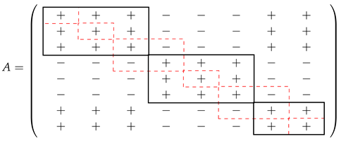
For example, for $k=3$ and $t=-1$, we have that the sign matrix of the inverse is $K_{3,-1}^{inv}=\mathrm{diag}(1,-1,1,1,-1,1,1,-1,1,1,-1,\dots )$. If we consider an $8\times 8$r-checkerboard matrix A with the sign structure given by $K_{3,-1}$, we have that

• where the black squares denote the diagonal blocks of positive entries. The dashed-line squares show how the interior of these blocks break into $1\times 1$ blocks and the $2\times 2$ blocks appearing when a positive block finishes and the next one starts. Hence, the sign structure of the inverse would be as follows:

For the particular case of 2-checkerboard matrices, we have that the two only possibilities for sign patterns are closely related. For a $K_{2,-1}$-checkerboard matrix, the associated signature would be ${\epsilon }_{2,-1}=(+1,-1,+1,-1\dots ,{(-1)}^{n-2})$. For a $K_{2,0}$-checkerboard matrix, its signature is ${\epsilon }_{2,0}=(-1,+1,-1,+1\dots ,{(-1)}^{n-1})$. Hence, we have that ${\epsilon }_{2,-1}=-{\epsilon }_{2,0}$, and we can obtain the following result by Theorem 3.1 of [16].

Corollary 2.

The inverse of a $K_{2,-1}$-checkerboard matrix is a $K_{2,0}$-checkerboard matrix.

Proof. 

If A is a $K_{2,-1}$-checkerboard matrix, then by Proposition 3.4, A is SBD with signature ${\epsilon }_{2,-1}$. By Theorem 3.1 of [16], a matrix is SBD with signature $\epsilon$ if and only if its inverse is SBD with signature $-\epsilon$. Therefore, $A^{-1}$ is SBD with signature $-{\epsilon }_{2,-1}={\epsilon }_{2,0}$, which implies, by Proposition 3.4, that $K_{2,0}{A}^{-1}{K}_{2,0}$ is nonsingular TP; so, $A^{-1}$ is a $K_{2,0}$-checkerboard matrix.    □

4. Bidiagonal Decomposition of Checkerboard Matrices

Given a $K_{r,t}$-checkerboard matrix A, we can multiply it from left and right by sign matrix $K_{r,t}$ to obtain a nonsingular TP matrix. Hence, their bidiagonal decompositions are related by the following formula:

$$\begin{array}{cc}\hfill \left|A\right|& =K_{r,t}A{K}_{r,t}=K_{r,t}{F}_{n-1}\cdots F_{1}D{G}_1\cdots G_{n-1}{K}_{r,t}\hfill \\ \hfill & =\left(K_{r,t}{F}_{n-1}{K}_{r,t}\right)\cdots \left(K_{r,t}{F}_1{K}_{r,t}\right)\left(K_{r,t}D{K}_{r,t}\right)\left(K_{r,t}{G}_1{K}_{r,t}\right)\cdots \left(K_{r,t}{G}_{n-1}{K}_{r,t}\right).\hfill \end{array}$$

(9)

If we know the bidiagonal decomposition of nonsingular TP matrix $K_{r,t}A{K}_{r,t}=\left|A\right|$, we can obtain the bidiagonal decomposition of A thanks to formula (9). This formula also allows us to apply some of the HRA algorithms known for nonsingular TP matrices to this class of matrices, according to [16]. For nonsingular TP matrices, accurate computations can be achieved using bidiagonal decomposition (Theorem 2) as a parametrization. In [13,15], Plamen Koev designed algorithms to solve various linear algebra problems with nonsingular TP matrices with HRA by taking the bidiagonal decomposition as input. These algorithms have been implemented and are available in the library TNTool for use in Matlab and Octave. This library also contains later contributions by other authors and can be downloaded from Koev’s personal website [17]. For $K_{r,t}$-checkerboard matrices, we can perform the following:

• Computing the eigenvalues of $\left|A\right|$ with HRA with the function TNEigenvalues in TNTool. The eigenvalues of A are the same, since they are similar matrices.
• Computing the singular values of $\left|A\right|$ with HRA using the function TNSingularValues. These singular values are also equal to the singular values of A, since $\left|A\right|$ and A coincide up to unitary matrices.
• Computing the inverse of $\left|A\right|$ with HRA with the function TNInverseExpand presented in Section 4 of [6] and available in TNTool. Then, we can obtain the inverse of A with HRA, since $A^{-1}=K_{r,t}{\left|A\right|}^{-1}{K}_{r,t}$.
• Solving the system of linear equations $Ax=b$ with HRA whenever $K_{r,t}b$ has an alternating pattern of signs, since $Ax=b$ is equivalent to $K_{r,t}A{K}_{r,t}\left(K_{r,t}x\right)=K_{r,t}b$, i.e., $\left|A\right|y=K_{r,t}b$, where $y=K_{r,t}x$, using the function TNSolve.

5. Intervals of Checkerboard Matrices

This section will present a result on intervals of checkerboard matrices. Given diagonal matrix J and two $n\times n$ matrices B and C, we can define the checkerboard ordering associated to J, ${\le }^{*}$. We say that $B{\le }^{*}C$ if $JBJ\le JCJ$, where ≤ is the usual entry-wise inequality between two matrices. This ordering has proven to be quite useful in characterizing intervals of TP matrices. In [18], the following theorem, which identifies intervals of nonsingular TP matrices, was proven.

Theorem 3.

Let B and C be $n\times n$ nonsingular TP matrices satisfying $B{\le }^{*}C$, i.e., $JBJ\le JCJ$. If A is an $n\times n$ matrix such that $B{\le }^{*}A{\le }^{*}C$, then A is nonsingular TP.

This idea has been extended to find orderings associated to SBD matrices in [19], and here, we analyze orderings for the case of checkerboard matrices. If a given $n\times n$ matrix A is a $K_{r,t}$-checkerboard matrix, we know that $K_{r,t}A{K}_{r,t}$ is nonsingular TP. Hence, we define the following ordering for $K_{r,t}$-checkerboard matrices.

Definition 5.

Given two $n\times n$ matrices, A and B, we define the ordering ${\le }^{r,t}$ as $A{\le }^{r,t}B$ if $J{K}_{r,t}A{K}_{r,t}J\le J{K}_{r,t}B{K}_{r,t}J$.

Now, we present a result on intervals of $K_{r,t}$-checkerboard matrices based on the ordering ${\le }^{r,t}$.

Proposition 3.

Let B and C be $n\times n$$K_{r,t}$-checkerboard matrices satisfying $B{\le }^{r,t}C$, i.e., $J{K}_{r,t}B{K}_{r,t}J\le J{K}_{r,t}C{K}_{r,t}J$. If A is an $n\times n$ matrix such that $B{\le }^{r,t}A{\le }^{r,t}C$, then A is a $K_{r,t}$-checkerboard matrix.

Proof. 

Since B and C are $K_{r,t}$-checkerboard matrices, we have that $K_{r,t}B{K}_{r,t}$ and $K_{r,t}C{K}_{r,t}$ are nonsingular TP matrices that satisfy $J\left(K_{r,t}B{K}_{r,t}\right)J\le J\left(K_{r,t}A{K}_{r,t}\right)J\le J\left(K_{r,t}C{K}_{r,t}\right)J$ for an $n\times n$ matrix A. Hence, by Theorem 3, $K_{r,t}A{K}_{r,t}$ is a nonsingular TP matrix, or equivalently, A is a $K_{r,t}$-checkerboard matrix.    □

6. Integer Examples

Many examples of TP matrices are ill conditioned. For instance, the symmetric Pascal matrix, whose $(i,j)$-th entry is the binomial coefficient $\left(\genfrac{}{}{0pt}{}{i+j-2}{j-1}\right)$ is a well-known example of ill-conditioning. However, the symmetric Pascal matrix admits a really simple representation in terms of the bidiagonal decomposition: all the nonzero entries of this factorization are ones. Hence, many linear algebra problems can be solved accurately with the Pascal matrix if we use algorithms that take the bidiagonal decomposition as input.

In this section, we are going to illustrate some examples of r-checkerboard matrices that admit an easy representation in terms of bidiagonal decomposition with integer entries.

6.1. Generalized Pascal Matrix

Our first example comes from an extension of the Pascal matrix depending on a parameter $x\in \mathbb{R}$. The generalized $K_{r,t}$-checkerboard Pascal matrix of the first kind, $S{P}_n\left[x\right]$, is defined as the triangular matrix

$${\left(S{P}_n\left[x\right]\right)}_{ij}={(-1)}^{\lfloor \frac{i+t}{r}\rfloor +\lfloor \frac{j+t}{r}\rfloor }{x}^{i-j}\left(\genfrac{}{}{0pt}{}{i-1}{j-1}\right),i\ge j$$

and the symmetric generalized Pascal matrix, $S{R}_n\left[x\right]$, is defined as

$${\left(S{R}_n\left[x\right]\right)}_{ij}={(-1)}^{\lfloor \frac{i+t}{r}\rfloor +\lfloor \frac{j+t}{r}\rfloor }{x}^{i+j-2}\left(\genfrac{}{}{0pt}{}{i+j-2}{j-1}\right).$$

(10)

These matrices are the signed counterparts of the generalized Pascal matrix, $P_n\left[x\right]:=\left|S{P}_n\left[x\right]\right|$, and the symmetric generalized Pascal matrix, $R_n\left[x\right]:=\left|S{R}_n\left[x\right]\right|$ (see [20]). Their bidiagonal decomposition are

$${\left(\mathcal{BD}\left(S{P}_n\left[x\right]\right)\right)}_{ij}=\left\{\begin{array}{cc}1,\hfill & \mathrm{if}i=j,\hfill \\ {\epsilon }_{i-1}x,\hfill & \mathrm{if}i>j,\hfill \\ 0,\hfill & \mathrm{if}i<j.\hfill \end{array}\right.$$

$${\left(\mathcal{BD}\left(S{R}_n\left[x\right]\right)\right)}_{ij}=\left\{\begin{array}{cc}{x}^{2(i-1)},\hfill & \mathrm{if}i=j,\hfill \\ {\epsilon }_{i-1}x,\hfill & \mathrm{if}i>j,\hfill \\ {\epsilon }_{j-1}x,\hfill & \mathrm{if}i<j,\hfill \end{array}\right.$$

(11)

respectively, where ${\epsilon }_i=\pm 1$ is given by (8) for $i=1,\dots ,n-1$. For the case $x\in \mathbb{Z}$, we have that these are examples of integer matrices.

6.2. Matrices of Stirling Numbers

Our next example comes from matrices of Stirling numbers. The Stirling numbers of the first kind ($s_{i,j}$) are the coefficients of the expansion of the falling factorial ${\left(x\right)}_n={\prod }_{k=0}^{n-1}(x-k)$, i.e., ${\left(x\right)}_n={\sum }_{k=0}^n{s}_{n,k}{x}^k$, where ${\left(x\right)}_n={\prod }_{k=0}^{n-1}(x-k)$. Let us recall that the Stirling numbers of the first kind can be calculated using the following recurrence relation:

$$s_{n+1,k}=s_{n,k-1}-n·s_{n,k},$$

where $s_{00}=1,s_{n0}=0$ for $n>0$, and $s_{0k}=0$ for $k>0$. Then, matrix $S={\left(s_{ij}\right)}_{1\le i,j\le n}$ is a $K_{1,-1}$-checkerboard matrix whose bidiagonal decomposition is given by

$${\left(\mathcal{BD}\left(S\right)\right)}_{ij}=\left\{\begin{array}{cc}1,& i=j,\\ -(i-j),& i>j,\\ 0,& \mathrm{otherwise}.\end{array}\right.$$

Matrix S is the inverse of a nonsingular TP matrix. That TP matrix is precisely the matrix whose entries are Stirling numbers of the second kind. Let us recall that the Stirling number of the second kind, $b_{n,k}$, counts the different partitions of a set of n elements into k non-empty subsets. Hence, these numbers can be obtained by using the recurrence relation

$$b_{n+1,k}=b_{n,k-1}+k·b_{n,k},$$

with the initial conditions $b_{00}=1,b_{n0}=0$ for $n>0$, and $b_{0k}=0$ for $k>0$. Then, matrix $B={\left(b_{ij}\right)}_{1\le i,j\le n}$ is a nonsingular TP matrix whose bidiagonal decomposition takes the following form:

$${\left(\mathcal{BD}\left(B\right)\right)}_{ij}=\left\{\begin{array}{cc}1,& i=j,\\ j,& i>j,\\ 0,& \mathrm{otherwise}.\end{array}\right.$$

7. Numerical Experiments

In [13], Koev introduced methods to calculate the eigenvalues and the singular values of A and the solution of linear systems of equations $Ax=b$, where b has a pattern of alternating signs from the parameterization $\mathcal{BD}\left(A\right)$ for the case where A is a TP matrix. These algorithms provide approximations to the solutions of these algebraic problems with HRA if $\mathcal{BD}\left(A\right)$ is obtained with HRA. In addition, in [6], Marco and Martínez developed an algorithm to calculate, with HRA, the inverse $A^{-1}$ under the same previous hypotheses. In the software library TNTool, available in [17], these four algorithms are implemented with Matlab. The names of the corresponding functions are TNEigenvalues, TNSingularValues, TNInverseExpand, and TNSolve. They require, as input argument, bidiagonal decomposition $\mathcal{BD}\left(A\right)$ of A, given by (7), with HRA. In addition, TNSolve needs vector b of the system of linear equations $Ax=b$ as a second argument. Regarding computational cost, the algorithms are at least as fast as the usual algorithms for solving these algebraic problems, as shown in the following:

• TNInverseExpand and TNSolve have both a computational cost of $\mathcal{O}\left(n^2\right)$ elementary operations.
• TNEigenValues and TNSingularValues both require $\mathcal{O}\left(n^3\right)$ elementary operations.

In order to illustrate the theoretical results, we considered the square matrices $S{R}_n[1/2]$ of order $n=5,10,\dots ,50$ defined by (10), i.e.,

$${\left(S{R}_n[1/2]\right)}_{ij}={(-1)}^{\lfloor \frac{i-1}{2}\rfloor +\lfloor \frac{j-1}{2}\rfloor }\frac{1}{2^{i+j}}\left(\genfrac{}{}{0pt}{}{i+j}{j}\right).$$

Table 1. Condition numbers of $S{R}_n[1/2]$.

n	$\mathit{k}\left({\mathit{SR}}_{\mathit{n}}[1/2]\right)$
5	5.44 × ${10}^3$
10	2.37 × ${10}^8$
15	1.11 × ${10}^{13}$
20	5.77 × ${10}^{17}$
25	3.06 × ${10}^{22}$
30	1.63 × ${10}^{27}$
35	8.96 × ${10}^{31}$
40	4.97 × ${10}^{36}$
45	2.74 × ${10}^{41}$
50	1.54 × ${10}^{46}$

shows the condition numbers $k\left(A\right):={\parallel A\parallel }_{\infty }{\parallel A^{-1}\parallel }_{\infty }$ of these matrices. It can be observed that these matrices are very ill conditioned. So, accurate results cannot be expected when using the usual algorithms for solving algebraic problems with them.

It can be observed that $S{R}_n[1/2]$ is a $K_{r,t}$-checkerboard matrix. In particular, it can be seen that $K_{2,-1}\left(S{R}_n[1/2]\right)K_{2,-1}=R_n[1/2]>0$, where $R_n[1/2]$ is the symmetric generalized Pascal matrix defined by the absolute value of (10) for $x=1/2$ and $K_{2,-1}$ is the order n matrix given by (4). Since $R_n[1/2]$ is a TP matrix, taking into account the discussion in Section 4, the singular values and the inverse of $S{R}_n[1/2]$, as well as the solution of systems $S{R}_n[1/2]x=b$, whenever $K_{2,-1}b$ has an alternating pattern of signs, can be computed with HRA. Observe that since $R_n[1/2]$ is a symmetric matrix, the eigenvalues and the singular values of $R_n[1/2]$ coincide. Since $K_{2,-1}^{-1}=K_{2,-1}$, the same applies to matrices $S{R}_n[1/2]$.

The bidiagonal decomposition ($\mathcal{BD}\left(R_n\left[x\right]\right)$) of a generalized symmetric Pascal matrix $R_n\left[x\right]$ can be computed with HRA for all $x>0$ by (11) (taking the case where ${\epsilon }_j=1$ for $j=1,\dots ,n-1$). We implemented the algorithm for the computation of this bidiagonal decomposition in the Matlab function TNBDGPascalSym.

First, by using TNBDGPascalSym in Matlab, we calculated the bidiagonal decomposition ($\mathcal{BD}\left(R_n[1/2]\right)$) with high relative accuracy. Then, we computed approximations to the singular values of $R_n[1/2]$ by using TNSingularValues with $\mathcal{BD}\left(R_n[1/2]\right)$ as input argument. Approximations to these singular values were also obtained with the Matlab function svd. In order to illustrate the accuracy of the approximations to the singular values computed by the two methods, the singular values of $S{R}_n[1/2]$ were also calculated with Mathematica using a precision of one hundred digits. Then, the relative errors for the approximations to the singular values obtained by both methods were computed, taking the singular values obtained with Mathematica as the exact singular values. These relative errors showed that the approximations of all the singular values calculated by using TNBDGPascalSym are highly accurate and that the approximations of the lower singular values computed by using the Matlab function svd are not very accurate. It was also observed that the lower the singular value is, the less accurate the approximation provided by svd is. To demonstrate this fact, the relative errors of the approximations to the smallest singular value of the considered examples ($S{R}_n[1/2]$, $n=5,10,\dots ,50$), obtained by both svd and TNSingularValues, are shown in Figure 1. From the results in that figure, it can be concluded that our method produces very accurate results, as opposed to the inaccurate results obtained with svd.

Approximations to ${\left(S{R}_n[1/2]\right)}^{-1}$, $n=5,10,\dots ,50$, were also obtained by using Matlab with inv and by using TNInverseExpand together with TNBDGPascalSym. The exact inverses, ${\left(S{R}_n[1/2]\right)}^{-1}$, were obtained with Mathematica using exact arithmetic. Then, the corresponding component-wise relative errors were computed. The mean relative errors are shown in Figure 2a, and the maximum relative errors are shown in (b). In this case, it is also clear that the accuracy of the results provided by TNInverseExpand is significantly better than that of the results provided by inv.

Finally, we considered the systems of linear equations $S{R}_n[1/2]x=b_n$, $n=5,10,\dots ,50$ such that $K_{2,-1}{b}_n$ has an alternating pattern of signs and with entries whose absolute value is an integer randomly chosen in the interval $[1,1000]$. Then, approximations to the solution of these linear systems were computed in two ways: the first one, by using the Matlab command A\b, and the second one, by solving the system $|S{R}_n[1/2]|y=K_{2,-1}{b}_n$ with TNSolve and then computing the solution of the original system as $x=K_{2,-1}y$. The exact solutions of these systems were computed with Mathematica; then, the component-wise relative errors for both approximations were calculated. The mean relative errors are shown in Figure 3a, and the maximum relative errors are shown in (b). The results obtained with the HRA algorithms are much better from the point of view of accuracy than the results obtained with the usual Matlab method.

In order to compare the computation time of the HRA methods with that of the usual methods, we solved the three algebraic problems considered in this section for $S{R}_{50}[1/2]$ one hundred times.

Table 2. Average computation time in seconds.

	Inverse	Linear System	Singular Values
HRA methods	6.32 × ${10}^{-4}$	1.34 × ${10}^{-5}$	3.90 × ${10}^{-3}$
Usual methods	2.06 × ${10}^{-4}$	1.95 × ${10}^{-4}$	8.07 × ${10}^{-5}$

shows the average computation time for each one of the algebraic problems.

8. Conclusions

We introduce the class of block checkerboard pattern matrices, which are matrices with a regular pattern of signs for which a generalized Perron–Frobenius type theorem is satisfied. We consider bidiagonal decomposition of checkerboard matrices for achieving linear algebra computations with high relative accuracy (HRA). These HRA computations include the calculation of all eigenvalues and all singular values, the calculation of the inverses, and the solution of some associated linear systems. We also introduce a new order relation for matrices, deriving a result on intervals of block checkerboard matrices. We present new families of matrices with integer entries, which can be used as test matrices to check the accuracy of linear algebra algorithms. Numerical examples illustrate the accuracy of the presented methods compared with standard methods for the abovementioned linear algebra computations.