Existence of Traveling Waves of a Diffusive Susceptible–Infected–Symptomatic–Recovered Epidemic Model with Temporal Delay

Abstract

The aim of this article is to investigate the existence of traveling waves of a diffusive model that represents the transmission of a virus in a determined population composed of the following populations: susceptible $\left(S\right),$ infected $\left(I\right),$ asymptomatic $\left(A\right)$, and recovered $\left(R\right).$ An analytical study is performed, where the existence of solutions of traveling waves in a bounded domain is demonstrated. We use the upper and lower coupled solutions method to achieve this aim. The existence and local asymptotic stability of the endemic ($E_e$) and disease-free $\left(E_0\right)$ equilibrium states are also determined. The constructed model includes a discrete-time delay that is related to the incubation stage of a virus. We find the crucial basic reproduction number ${\mathcal{R}}_0$, which determines the local stability of the steady states. We perform numerical simulations of the model in order to provide additional support to the theoretical results and observe the traveling waves. The model can be used to study the dynamics of SARS-CoV-2 and other viruses where the disease evolution has a similar behavior.

1. Introduction

Mathematical models have been extensively used to study the dynamics of many infectious diseases [1]. It is common to use differential equations to construct these models. The most well-known models are based on ordinary differential equations (ODEs), partial differential equations (PDEs), and delay differential equations (DDEs) [2,3,4,5]. The SIR (susceptible–infected–recovered) model is by far the most commonly used mathematical model based on differential equations [1]. Recently, the SAIR model, or its variants, has been used to address well-known asymptomatic cases [6,7,8,9]. In [10], a SIR model that incorporates awareness and a time delay to account for the latent stage was studied. These previous studies have used ODEs, as specific spatial effects were not considered.

Often in mathematical epidemiology, models that consider the spatial component, where individuals live, are usually described using partial differential equations. This is justified by the movement of individuals from one place to another, either within a region or through the emigration of the population to other regions through its borders. Another important variable in modeling infectious diseases is the delay in the appearance of the symptoms of the disease after individuals become infected. In [11], the authors proposed an epidemic SIR mathematical model with spatial diffusion and time delay. The authors investigated the existence of traveling waves in their proposed SIR model. In addition, they determined the stationary states and analyzed the existence of waves through the existence of upper and lower solutions. Other works have incorporated discrete-time delays in partial differential equations [12,13,14]. For instance, in [12], the authors analyzed the existence of wavefront solutions using a monotonous iteration scheme for the wave system. The authors proved that the wave system has a solution if the quasi-monotonicity (QM) condition is satisfied.

The incorporation of time delays can make the mathematical models more realistic, but then these models and their analysis become more complex. Thus, time delays can be incorporated into reaction-diffusion systems, but then classical techniques such as the phase plane cannot be applied to guarantee the existence of the solution. However, by applying the monotonous iteration technique, the existence of a traveling wave solution was demonstrated for a reaction-diffusion model with delays [13]. The monotonous iteration technique was demonstrated in [12,14]. Another interesting work was presented in [15]. The authors found and proved the existence of traveling waves when they analyzed an SEIR-type model represented by a system of reaction-diffusion equations. In addition, the authors computed the basic reproduction number, which is a threshold parameter for the long-term dynamics, and used it to prove the existence of traveling waves.

In this direction of epidemiological applications, in [16], the authors analyzed the role of population mobility in the transmission of coronavirus disease 2019 (COVID-19) using a nonlinear parabolic system. The authors presented alternatives to control the transmission of the virus by applying restrictions such as the closure of borders, reduction of travel, and interruption of human mobility. In another interesting work [17], the authors presented an epidemiological SEIR-type model with reaction-diffusion terms, nonlinear incidence, and distributive delay. The authors applied the Lyapunov function methodology and the basic reproduction number to analyze the stability of the stationary states.

In this paper, we present a SAIR-type epidemiological model based on a system of partial differential equations, incorporating a discrete-time delay to mimic the virus’s incubation period within a host and the time it takes for a person to become infected [10,18,19,20,21]. The spatial effect is justified due to people’s mobility and the spread of the virus [6,16,22,23]. Thus, the main contributions of this paper are the introduction of spatial effects in conjunction with the time delay due to the latent stage of individuals. Moreover, the model includes asymptomatic cases and considers the possibility of death for asymptomatic individuals. In addition, we find the crucial basic reproduction number ${\mathcal{R}}_0$, which determines the local stability of the steady states. In general, this theoretical result is more complex to achieve in mathematical models that include spatial effects and time delays compared to classical models based on ODEs.

There are different ways to introduce a discrete-time delay in an epidemiological mathematical model. This delay takes into account the fact that when a susceptible individual has effective contact with an infected individual, the susceptible person does not become infectious right away, i.e., they are unable to spread the virus [24,25,26,27,28,29]. In this article, we use a particular approach to introduce the time delay that has been used in several previous papers related to the mathematical modeling of epidemics [11,30,31]. We aim to analyze the existence and uniqueness of a traveling wave that connects the two equilibrium points of the system. In addition, we will analyze the stability of the stationary points of the model. The proposed mathematical model represents the transmission of a virus in a determined population composed of susceptible $\left(S\right),$ infected $\left(I\right),$ asymptomatic $\left(A\right)$, and recovered $\left(R\right)$ individuals. As with any real-world mathematical model, there are simplifications and assumptions. However, this type of study provides additional insights into the dynamics of different diseases [1,26,32]. We perform an analytical study, where the existence of solutions of traveling waves in a bounded domain is demonstrated. We use a method that is based on the upper and lower coupled solutions to prove this existence. The existence and local asymptotic stability of the endemic ($E_e$) and disease-free $\left(E_0\right)$ equilibrium states are determined. It should be mentioned that the proposed mathematical model can be used to study the dynamics of SARS-CoV-2 and other viruses where the disease status evolution is similar.

This paper is organized as follows. Section 2 introduces the constructed model and Section 3 provides the mathematical analysis of the existence and uniqueness of the solution. The stability of the equilibrium points is then discussed in Section 4. In Section 5, numerical simulations of the solutions are presented, and finally, in Section 6, the conclusions of this study are given.

2. Materials and Methods

In this section, we present the most important elements that are often used to design new epidemiological mathematical models and the mathematical tools that can be used to demonstrate that the model is well posed.

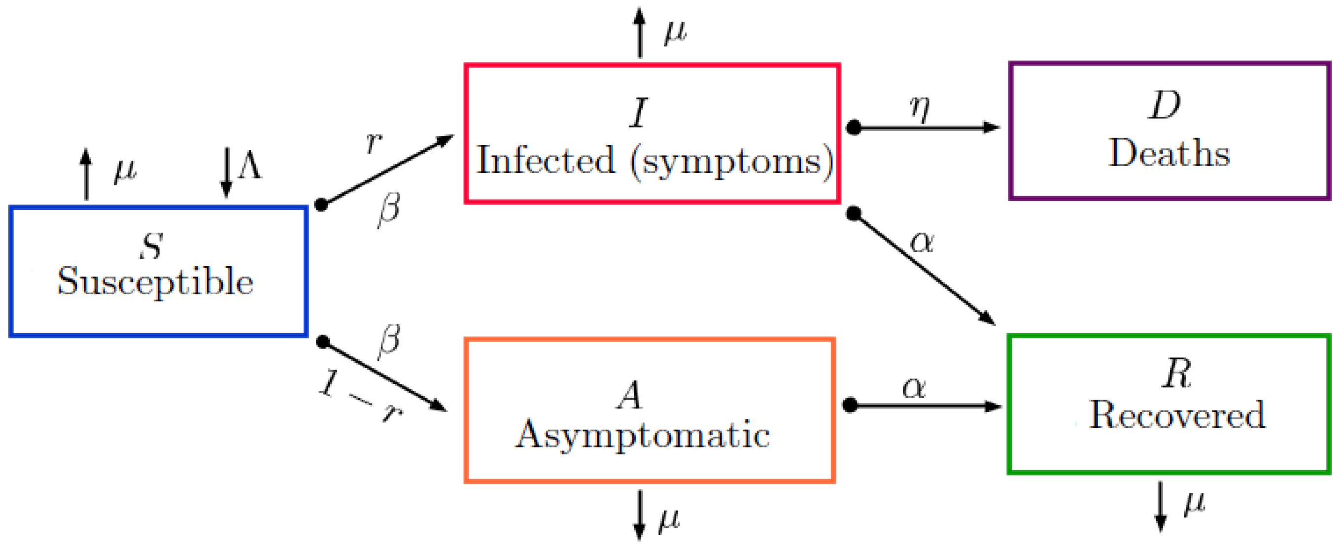
2.1. Mathematical Model

In this subsection, we present a mathematical model that is based on a system of partial differential equations with a discrete-time delay, where the population has been subdivided into the following subpopulations: susceptible (S) people who do not have the virus but can be infected, infected (I) people with symptoms of the disease who have the ability to infect susceptible individuals, asymptomatic $\left(A\right)$ infected people who can transmit the disease but do not present symptoms of the disease, and finally, recovered (R) people who have had the disease but do not transmit it.

Let us consider a bounded domain $\mathsf{\Omega }\subset R$ and a time interval $[0,T].$ We assume that $N:\overline{\mathsf{\Omega }}\times [0,T]\to \mathbb{R}$ is a non-negative function representing the spatio-temporal density of the population. That is, $N(x,t)$ denotes the number of individuals over the point $xin\overline{\mathsf{\Omega }}$ at the instant $tin[0,T]$. It is also assumed that $S,I,A,R:\overline{\mathsf{\Omega }}\times [0,T]\to \mathbb{R}$ are non-negative functions such that $N(x,t)=S(x,t)+I(x,t)+A(x,t)+R(x,t)$, and they describe the densities of the subpopulations that interact in this model. These functions are given as follows:

• $S(x,t)$ is the population susceptible to the virus in space and time;
• $I(x,t)$ is the infected population presenting symptoms of the disease and transmitting the virus in space and time;
• $A(x,t)$ is the population infected by the virus that does not present symptoms, that is, it is asymptomatic and transmits the virus in space and time;
• $R(x,t)$ is the population that has recovered from the disease and does not present symptoms of the disease but is under medical treatment.

With the above considerations, we present a model governed by partial differential equations, where the interaction and flow of the subpopulations involved in this class of epidemiological models are shown in Figure 1. Thus, one has

$$\begin{array}{cc}\hfill {\displaystyle \frac{\partial S(x,t)}{\partial t}}=& \mathsf{\Lambda }-\beta S(x,t)\left[I\right(x,t-\tau )+A(x,t-\tau \left)\right]-\mu S(x,t)\hfill \\ \hfill & +\nabla ·\left[{\nu }_S\nabla S(x,t)\right],\hfill \\ \hfill {\displaystyle \frac{\partial I(x,t)}{\partial t}}=& r\beta S(x,t)\left[I\right(x,t-\tau )+A(x,t-\tau \left)\right]-\mu I(x,t)-\eta I(x,t)\hfill \\ \hfill & -\alpha I(x,t)+\nabla ·\left[{\nu }_I\nabla I(x,t)\right],\hfill \\ \hfill {\displaystyle \frac{\partial A(x,t)}{\partial t}}=& (1-r)\beta S(x,t)\left[I\right(x,t-\tau )+A(x,t-\tau \left)\right]-\mu A(x,t)\hfill \\ \hfill & -\alpha A(x,t)+\nabla ·\left[{\nu }_A\nabla A(x,t)\right],\hfill \\ \hfill {\displaystyle \frac{\partial R(x,t)}{\partial t}}=& \alpha [I(x,t)+A(x,t)]-\mu R(x,t)+\nabla ·\left[{\nu }_R\nabla R(x,t)\right],\hfill \end{array}$$

(1)

where $\nabla =\left(\frac{\partial }{\partial x}\right)$ is the vector differential operator; $\mathsf{\Lambda }$ represents the rate of new people entering the susceptible population; $\alpha$ is the recovery rate; $\eta$ is the mortality rate caused by infection; $\beta$ is the contagion rate; $\mu$ is the general natural mortality rate; r is the proportion of people who become infected and present symptoms; and ${\nu }_S,{\nu }_A,{\nu }_I,{\nu }_R$ are diffusion parameters, indicating the space and time mobility of the susceptible, infected, and recovered individuals on those classes, respectively [33].

Figure 1. Diagram of the mathematical model (1) based on a system of partial differential equations with a discrete-time delay $\tau$.

The mathematical model (1) is considered closed. Therefore, we consider Neumann-type boundary conditions. That is, we assume that $\mathbf{n}(x,t)$ is the unit normal vector of $\overline{\mathsf{\Omega }}$ to the point $(x,t)\in \partial \mathsf{\Omega }\times [0,T]$, where $\partial \mathsf{\Omega }$ represents the border of $\mathsf{\Omega }$ and $\mathcal{C}:=C(\mathsf{\Omega }\times [-\tau ,0],{\mathbb{R}}^4)$ for $\tau >0$ represents the set of continuous functions defined in $\mathsf{\Omega }\times [-\tau ,0]$. Due to the above, the initial and boundary conditions of the mathematical model (1) are as follows:

$$\begin{array}{c}\hfill \left\{\begin{array}{cc}\nabla u(x,t)·\mathbf{n}\left(t\right)=\mathbf{0}\hfill & (x,t)\in \partial \mathsf{\Omega }\times (0,T];\hfill \\ u_0(x,\theta )=\phi (x,\theta )\hfill & \phi \in \mathcal{C},\hfill \end{array}\right.\end{array}$$

(2)

where $u={(S,I,A,R)}^T$ and $\phi ={({\phi }_1,{\phi }_2,{\phi }_3,{\phi }_4)}^T$ such that ${\phi }_i$ is a non-negative real function for $i=1,2,3,4$.

2.2. Existence of Equilibrium States

Now, we analyze the equations of system (1) with conditions (2) to determine the existence of a disease-free equilibrium and an endemic equilibrium. In this way, the stability of these steady states is shown. The Neumann boundary conditions are given in (2) and indicate that

$$\frac{\partial s(x,t)}{\partial n}=\frac{\partial I(x,t)}{\partial n}=\frac{\partial A(x,t)}{\partial n}=\frac{\partial R(x,t)}{\partial n}=0\forall (x,t)\in \partial \mathsf{\Omega }\times [0,T],$$

where $\frac{\partial }{\partial n}$ denotes the normal outward derivative over $\partial \mathsf{\Omega }$. These boundary conditions mean that subpopulations do not cross the boundary $\partial \mathsf{\Omega }$.

The disease-free equilibrium $E_0$ is obtained by setting $A=I=R=0$. Thus,

$$\begin{array}{c}\hfill E_0\left(\frac{\mathsf{\Lambda }}{\mu },0,0,0\right).\end{array}$$

(3)

Now, if we assume $I,A>0$, the solution of the following system represents the endemic stationary state, i.e,

$$\begin{array}{cc}\hfill \mathsf{\Lambda }-\beta S^e(I^e+A^e)-\mu S^e& =0,\hfill \\ \hfill r\beta S^e(I^e+A^e)-(\mu +\alpha +\eta )I^e& =0,\hfill \\ \hfill (1-r)\beta S^e(I^e+A^e)-(\mu +\alpha )A^e& =0,\hfill \\ \hfill \alpha (I^e+A^e)-\mu R^e& =0.\hfill \end{array}$$

(4)

From the second and third equations of (4) and dividing by $I^e>0$, one obtains

$$\begin{array}{cc}\hfill r\beta S^e(1+\frac{A^e}{I^e})-(\mu +\alpha +\eta )& =0,\hfill \\ \hfill (1-r)\beta S^e(1+\frac{A^e}{I^e})-(\mu +\alpha )\frac{A^e}{I^e}& =0.\hfill \end{array}$$

(5)

Next, from (5), one obtains

$$\begin{array}{c}\hfill \beta S^e(1+\frac{A^e}{I^e})=\frac{\mu +\alpha +\eta }{r}.\end{array}$$

(6)

We can obtain from (6) and the second equation of (5) that

$$\begin{array}{c}\hfill (1-r)\left(\frac{\mu +\alpha +\eta }{r}\right)=(\mu +\alpha )\frac{A^e}{I^e}\Rightarrow \frac{(1-r)(\mu +\alpha +\eta )}{r(\mu +\alpha )}=\frac{A^e}{I^e}.\end{array}$$

(7)

Thus,

$$\begin{array}{cc}\hfill & \beta S^e\left(1+\frac{(1-r)(\mu +\alpha +\eta )}{r(\mu +\alpha )}\right)=\frac{\mu +\alpha +\eta }{r},\hfill \\ \hfill & \beta S^e\left(\frac{r(\mu +\alpha )+(1-r)(\mu +\alpha +\eta )}{r(\mu +\alpha )}\right)=\frac{\mu +\alpha +\eta }{r},\hfill \\ \hfill & S^e=\frac{(\mu +\alpha )(\mu +\alpha +\eta )}{\beta (\mu +\alpha +(1-r\left)\eta \right)}.\hfill \end{array}$$

Now, we can replace the first equation of (4) and substitute $S^e$ into the second and third equations of (4) to obtain $I^e$ and $A^e$ as

$$\begin{array}{cc}\hfill I^e& =\frac{r\mathsf{\Lambda }}{\mu +\alpha +\eta }-\frac{r\mu (\mu +\alpha )}{\beta (\mu +\alpha +(1-r\left)\eta \right)}=\frac{r\left[\mathsf{\Lambda }\beta \right(\mu +\alpha +(1-r)\eta )-\mu (\mu +\alpha \left)\right(\mu +\alpha +\eta \left)\right]}{\beta (\mu +\alpha +\eta )(\mu +\alpha +(1-r\left)\eta \right)}.\hfill \\ \hfill A^e& =\frac{(1-r)\mathsf{\Lambda }}{\mu +\alpha }-\frac{(1-r)\mu (\mu +\alpha +\eta )}{\beta (\mu +\alpha +(1-r\left)\eta \right)}\hfill \\ & =\frac{(1-r)\left[\mathsf{\Lambda }\beta \right(\mu +\alpha +(1-r)\eta )-\mu (\mu +\alpha \left)\right(\mu +\alpha +\eta \left)\right]}{\beta (\mu +\alpha )(\mu +\alpha +(1-r\left)\eta \right)}.\hfill \end{array}$$

Now, we define the following parameter

$$\begin{array}{c}\hfill {\mathcal{R}}_0=\frac{\mathsf{\Lambda }\beta (\mu +\alpha +(1-r\left)\eta \right)}{\mu (\mu +\alpha )(\mu +\alpha +\eta )}.\end{array}$$

(8)

With the above results, we have the following proposition:

Proposition 1.

If ${\mathcal{R}}_0>1,$ there is only one endemic state $E_e(S^e,I^e,A^e,R^e)$ of system (1) with the conditions given in (2), which is

$$\begin{array}{cc}\hfill S^e& =\frac{(\mu +\alpha )(\mu +\alpha +\eta )}{\beta (\mu +\alpha +(1-r\left)\eta \right)}=\frac{\mathsf{\Lambda }}{\mu {\mathcal{R}}_0},\hfill \\ \hfill I^e& =\frac{r\left[\mathsf{\Lambda }\beta \right(\mu +\alpha +(1-r)\eta )-\mu (\mu +\alpha \left)\right(\mu +\alpha +\eta \left)\right]}{\beta (\mu +\alpha +\eta )(\mu +\alpha +(1-r\left)\eta \right)}=\frac{\mathsf{\Lambda }r[{\mathcal{R}}_0-1]}{{\mathcal{R}}_0(\mu +\alpha +\eta )},\hfill \\ \hfill A^e& =\frac{(1-r)\left[\mathsf{\Lambda }\beta \right(\mu +\alpha +(1-r)\eta )-\mu (\mu +\alpha \left)\right(\mu +\alpha +\eta \left)\right]}{\beta (\mu +\alpha )(\mu +\alpha +(1-r\left)\eta \right)}=\frac{\mathsf{\Lambda }(1-r)[{\mathcal{R}}_0-1]}{{\mathcal{R}}_0(\mu +\alpha )},\hfill \\ \hfill R^e& =\frac{\alpha }{\mu }(I^e+A^e)=\frac{\alpha [{\mathcal{R}}_0-1]}{\beta }.\hfill \end{array}$$

3. Existence and Uniqueness of the Solution

Since model (1) represents an epidemiological model, from a biological point of view, it is important to analyze the epidemic waves generated when solutions propagate as traveling waves that move at a certain speed. Here, we show the existence of a single solution of model (1) with the conditions given in (2) (see Appendix A). We assume that the diffusion coefficients are constant. We simplify the notation by setting for $(x,t)\in \overline{\mathsf{\Omega }}\times [0,T]$, and $\tau >0$ the following: $S=S(x,t),I=I(x,t),A=A(x,t),R=R(x,t)$, and $N=N(x,t)$, $T_{\tau }=T(x,t-\tau ).$ Then, system (1) can be written as

$$\begin{array}{cc}\hfill {\displaystyle \frac{\partial S}{\partial t}}=& \mathsf{\Lambda }-\beta S{I}_{\tau }-\beta S{A}_{\tau }-\mu S+\nabla ·\left({\nu }_S\nabla S\right),\hfill \\ \hfill {\displaystyle \frac{\partial I}{\partial t}}=& r\beta S{I}_{\tau }+r\beta S{A}_{\tau }-(\mu +\eta +\alpha )I+\nabla ·\left({\nu }_I\nabla I\right),\hfill \\ \hfill {\displaystyle \frac{\partial A}{\partial t}}=& (1-r)\beta S{I}_{\tau }+(1-r)\beta S{A}_{\tau }-(\alpha +\mu )A+\nabla ·\left({\nu }_A\nabla A\right),\hfill \\ \hfill {\displaystyle \frac{\partial R}{\partial t}}=& \alpha I+\alpha A-\mu R+\nabla ·\left({\nu }_R\nabla R\right).\hfill \end{array}$$

(9)

We set $M(x,t)=\frac{\mathsf{\Lambda }}{\mu }-S(x,t).$ Then, system (9) is transformed into

$$\begin{array}{cc}\hfill {\displaystyle \frac{\partial M}{\partial t}}=& -\mu M+\beta \left(\frac{\mathsf{\Lambda }}{\mu }-M\right)(I_{\tau }+A_{\tau })+{\nu }_M\mathsf{\Delta }M,\hfill \\ \hfill {\displaystyle \frac{\partial I}{\partial t}}=& r\beta \left(\frac{\mathsf{\Lambda }}{\mu }-M\right)(I_{\tau }+A_{\tau })-(\alpha +\mu +\eta )I+{\nu }_I\mathsf{\Delta }I,\hfill \\ \hfill {\displaystyle \frac{\partial A}{\partial t}}=& (1-r)\beta \left(\frac{\mathsf{\Lambda }}{\mu }-M\right)(I_{\tau }+A_{\tau })-(\alpha +\mu )A+{\nu }_A\mathsf{\Delta }A,\hfill \\ \hfill {\displaystyle \frac{\partial R}{\partial t}}=& \alpha (I+A)-\mu R+{\nu }_R\mathsf{\Delta }R.\hfill \end{array}$$

(10)

System (10) has two stationary states. If ${\mathcal{R}}_0<1$ it is $\mathbf{0}={(0,0,0,0)}^T$, and for ${\mathcal{R}}_0>1$, it is $\mathbf{k}={(k_1,k_2,k_3,k_4)}^T$, where

$$\begin{array}{c}\hfill k_1=\frac{\mathsf{\Lambda }}{\mu }-S^e,k_2=I^e,k_3=A^e,k_4=R^e,k_i>0,i=1,2,3,4.\end{array}$$

(11)

Using the notation presented in [34] and substituting into (10), the solutions are given by

$$M(x,t)={\phi }_1\left(\frac{x}{c}+t\right),I(x,t)={\phi }_2\left(\frac{x}{c}+t\right),A(x,t)={\phi }_3\left(\frac{x}{c}+t\right),R(x,t)={\phi }_4\left(\frac{x}{c}+t\right),$$

and by setting $s=\frac{x}{c}+t$, one obtains the following system:

$$\begin{array}{cc}\hfill \frac{d_1}{c^2}{\varphi }_1^{″}\left(s\right)-{\varphi }_1^{\prime }\left(s\right)+f_1\left({\varphi }_s\right)& =0,\hfill \\ \hfill \frac{d_2}{c^2}{\varphi }_2^{″}\left(s\right)-{\varphi }_2^{\prime }\left(s\right)+f_2\left({\varphi }_s\right)& =0,\hfill \\ \hfill \frac{d_3}{c^2}{\varphi }_3^{″}\left(s\right)-{\varphi }_3^{\prime }\left(s\right)+f_3\left({\varphi }_s\right)& =0,\hfill \\ \hfill \frac{d_3}{c^2}{\varphi }_4^{″}\left(s\right)-{\varphi }_4^{\prime }\left(s\right)+f_4\left({\varphi }_s\right)& =0,\hfill \end{array}$$

(12)

where $d_1={\nu }_M$, $d_2={\nu }_I$, $d_3={\nu }_A$, $d_4={\nu }_R$, $\varphi ={({\varphi }_1,{\varphi }_2,{\varphi }_3,{\varphi }_4)}^T$, ${\varphi }_s\in C([-\tau ,0],{\mathbb{R}}^4)$ with ${\varphi }_s={({\varphi }_1^s,{\varphi }_2^s,{\varphi }_3^s,{\varphi }_4^s)}^T$; ${\varphi }_i^s\left(\theta \right)={\varphi }_i(s+\theta )$ and

$$\begin{array}{cc}\hfill f_1\left({\varphi }_s\right)& =-\mu {\varphi }_1^s\left(0\right)+\beta \left(\frac{\mathsf{\Lambda }}{\mu }-{\varphi }_1^s\left(0\right)\right)({\varphi }_2^s(-\tau )+{\varphi }_3^s(-\tau )),\hfill \\ \hfill f_2\left({\varphi }_s\right)& =r\beta \left(\frac{\mathsf{\Lambda }}{\mu }-{\varphi }_1^s\left(0\right)\right)[{\varphi }_2^s(-\tau )+{\varphi }_3^s(-\tau )]-(\alpha +\mu +\eta ){\varphi }_2^s\left(0\right),\hfill \\ \hfill f_3\left({\varphi }_s\right)& =(1-r)\beta \left(\frac{\mathsf{\Lambda }}{\mu }-{\varphi }_1^s\left(0\right)\right)[{\varphi }_2^s(-\tau )+{\varphi }_3^s(-\tau )]-(\alpha +\mu ){\varphi }_3^s\left(0\right),\hfill \\ \hfill f_4\left({\varphi }_s\right)& =\alpha ({\varphi }_2^s\left(0\right)+{\varphi }_3^s\left(0\right))-\mu {\varphi }_4^s\left(0\right),\hfill \end{array}$$

(13)

where $\varphi$ satisfies the following asymptotic boundary conditions:

$$\begin{array}{c}\hfill \underset{s\to -\infty }{lim}\varphi \left(s\right)=\mathbf{0},\underset{s\to \infty }{lim}\varphi \left(s\right)=\mathbf{k}.\end{array}$$

(14)

Let us show that the function $f={(f_1,f_2,f_3,f_4)}^T$ satisfies conditions ${\mathbf{A}}_{\mathbf{1}},{\mathbf{A}}_{\mathbf{2}},$ and ${\mathbf{A}}_{\mathbf{3}}$ given in (A4).

Proposition 2 (A₁).

Suppose that $f={(f_1,f_2,f_3,f_4)}^T$ and that $W(\mathsf{\Omega },{\mathbb{R}}^4)$ is like in (A3). Then, $f\left(\mathit{0}\right)=f\left(\mathit{k}\right)=\mathit{0}.$

Proof. 

The proof follows from (13). □

Proposition 3 (A₂).

$f_i$ satisfies the Lipschitz condition in $W([-\tau ,0],{\mathbb{R}}^4)$ for $i=1,2,3,4$.

Proof. 

Set $\varphi ,\psi \in W([-\tau ,0],{\mathbb{R}}^4)$. Then,

$$\begin{array}{cc}\hfill |f_1\left(\varphi \right)-f_1\left(\psi \right)|& =|-\mu {\varphi }_1\left(0\right)+\beta \left(\frac{\mathsf{\Lambda }}{\mu }-{\varphi }_1\left(0\right)\right)\left({\varphi }_2(-\tau )+{\varphi }_3(-\tau )\right)+\mu {\psi }_1\left(0\right)\hfill \\ & -\beta \left(\frac{\mathsf{\Lambda }}{\mu }-{\psi }_1\left(0\right)\right)[{\psi }_2(-\tau )+{\psi }_3(-\tau )]|\hfill \\ \hfill & \le \mu |{\psi }_1\left(0\right)-{\varphi }_1\left(0\right)|\hfill \\ & +\beta \left|\left(\frac{\mathsf{\Lambda }}{\mu }-{\varphi }_1\left(0\right)\right)[{\varphi }_2(-\tau )-{\varphi }_3(-\tau )]\right.-\left.\left(\frac{\mathsf{\Lambda }}{\mu }-{\psi }_1\left(0\right)\right)[{\psi }_2(-\tau )-{\psi }_3(-\tau )]\right|\hfill \\ \hfill & \le \mu |{\psi }_1\left(0\right)-{\varphi }_1\left(0\right)|+\frac{\beta \mathsf{\Lambda }}{\mu }\left(\right|{\varphi }_2(-\tau )-{\psi }_2(-\tau )|+|{\varphi }_3(-\tau )-{\psi }_3(-\tau )\left|\right)\hfill \\ \hfill & +\beta |-{\varphi }_1\left(0\right)({\varphi }_2(-\tau )+{\varphi }_3(-\tau ))+{\psi }_1\left(0\right)({\psi }_2(-\tau )+{\psi }_3(-\tau ))|\hfill \\ \hfill & \le \mu |{\psi }_1\left(0\right)-{\varphi }_1\left(0\right)|+\frac{\beta \mathsf{\Lambda }}{\mu }\left(\right|{\varphi }_2(-\tau )-{\psi }_2(-\tau )|+|{\varphi }_3(-\tau )-{\psi }_3(-\tau )\left|\right)\hfill \\ \hfill & +\beta |-{\varphi }_1\left(0\right){\varphi }_2(-\tau )-{\varphi }_1\left(0\right){\varphi }_3(-\tau )+{\psi }_1\left(0\right){\psi }_2(-\tau )+{\psi }_1\left(0\right){\psi }_3(-\tau )|.\hfill \end{array}$$

Thus, one obtains

$$\begin{array}{cc}\hfill |f_1\left(\varphi \right)-f_1\left(\psi \right)|& \le \mu |{\psi }_1\left(0\right)-{\varphi }_1\left(0\right)|+\frac{\beta \mathsf{\Lambda }}{\mu }\left(\right|{\varphi }_2(-\tau )-{\psi }_2(-\tau )|+|{\varphi }_3(-\tau )-{\psi }_3(-\tau )\left|\right)\hfill \\ \hfill & +\beta m_1|{\psi }_2(-\tau )-{\varphi }_2(-\tau )|+\beta m_2|{\psi }_1\left(0\right)-{\varphi }_1\left(0\right)|\hfill \\ & +\beta m_3|{\psi }_1\left(0\right)-{\varphi }_1\left(0\right)|+\beta m_1|{\psi }_3(-\tau )-{\varphi }_3(-\tau )|.\hfill \end{array}$$

Therefore, $|f_1\left(\varphi \right)-f_1\left(\psi \right)|\le L_1{\parallel \varphi -\psi \parallel }_W$, where $L_1=\mu +\frac{2\beta \mathsf{\Lambda }}{\mu }+2\beta m_1+\beta (m_2+m_3).$ In a similar process, for all $\varphi ,\psi \in W([-\tau ,0],{\mathbb{R}}^4)$, we can find the constants $L_i$, con $i=2,3,4$, such that $|f_i\left(\varphi \right)-f_i\left(\psi \right)|\le L_i{\parallel \varphi -\psi \parallel }_W$. □

Proposition 4 (A₃).

The function $f={(f_1,f_2,f_3,f_4)}^T$ holds the partial conditions of quasi-monotonicity (PQM) given in Definition A4, and $W([-\tau ,0],{\mathbb{R}}^4)$.

Proof. 

Consider $\psi ,\phi \in W([-\tau ,0],{\mathbb{R}}^4)$, with $\psi ={({\psi }_1,{\psi }_2,{\psi }_3,{\psi }_4)}^T,\phi ={({\phi }_1,{\phi }_2,{\phi }_3,{\phi }_4)}^T,$ and $0\le {\psi }_i\le {\phi }_i\le m_i$ for all $i=1,2,3,4.$ Moreover, suppose that

$$\begin{array}{c}\hfill {\phi }^{2,3}={({\phi }_1,{\psi }_2,{\psi }_3,{\phi }_4)}^T{\phi }^1={({\psi }_1,{\phi }_2,{\phi }_3,{\phi }_4)}^T,{\phi }^4={({\phi }_1,{\phi }_2,{\phi }_3,{\psi }_4)}^T.\end{array}$$

Set $\mathbf{m}={(m_1,m_2,m_3,m_4)}^T>\mathbf{k}$ such that $\frac{\mathsf{\Lambda }}{\mu }-m_i>0$. Then, $\frac{\mathsf{\Lambda }}{\mu }-{\phi }_i\left(0\right)\ge \frac{\mathsf{\Lambda }}{\mu }-m_i>0,$ and hence

$$\begin{array}{cc}\hfill f_1\left(\phi \right)-f_1\left(\psi \right)& =-\mu {\phi }_1\left(0\right)+\beta \left(\frac{\mathsf{\Lambda }}{\mu }-{\phi }_1\left(0\right)\right)[{\phi }_2(-\tau )+{\phi }_3(-\tau )]\hfill \\ & +\mu {\psi }_1\left(0\right)-\beta \left(\frac{\mathsf{\Lambda }}{\mu }-{\psi }_1\left(0\right)\right)[{\psi }_2(-\tau )+{\psi }_3(-\tau )]\hfill \\ \hfill & \ge -\mu {\phi }_1\left(0\right)+\beta \left(\frac{\mathsf{\Lambda }}{\mu }-{\phi }_1\left(0\right)\right)[{\psi }_2(-\tau )+{\psi }_3(-\tau )]\hfill \\ & +\mu {\psi }_1\left(0\right)-\beta \left(\frac{\mathsf{\Lambda }}{\mu }-{\psi }_1\left(0\right)\right)[{\psi }_2(-\tau )+{\psi }_3(-\tau )]\hfill \\ \hfill & \ge \mu ({\psi }_1\left(0\right)-{\phi }_1\left(0\right))+\beta \left({\psi }_1\left(0\right)-{\phi }_1\left(0\right)\right)[{\psi }_2(-\tau )+{\psi }_3(-\tau )].\hfill \end{array}$$

Now, since ${\psi }_2+{\psi }_3\le m_2+m_3$ and ${\psi }_1\left(0\right)-{\phi }_1\left(0\right)\le 0$, this implies that

$$({\psi }_1\left(0\right)-{\phi }_1\left(0\right))({\psi }_2(-\tau )+{\psi }_3(-\tau ))\ge ({\psi }_1\left(0\right)-{\phi }_1\left(0\right))(m_2+m_3).$$

Thus,

$$\begin{array}{cc}\hfill f_1\left(\phi \right)-f_1\left(\psi \right)& \ge \mu ({\psi }_1\left(0\right)-{\phi }_1\left(0\right))+\beta (m_2+m_3)({\psi }_1\left(0\right)-{\phi }_1\left(0\right))\hfill \\ & \ge [\mu +\beta (m_2+m_3)]({\psi }_1\left(0\right)-{\phi }_1\left(0\right)).\hfill \end{array}$$

Consider ${\beta }_1=\mu +\beta (m_2+m_3)>0$, then $f_1\left(\phi \right)-f_1\left(\psi \right)+{\beta }_1({\phi }_1\left(0\right)-{\psi }_1\left(0\right))\ge 0.$ Now,

$$\begin{array}{cc}\hfill f_2\left(\phi \right)-f_2\left({\phi }^{2,3}\right)& =r\beta \left(\frac{\mathsf{\Lambda }}{\mu }-{\phi }_1\left(0\right)\right)[{\phi }_2(-\tau )+{\phi }_3(-\tau )]-(\alpha +\mu +\eta ){\phi }_2\left(0\right)\hfill \\ \hfill & -r\beta \left(\frac{\mathsf{\Lambda }}{\mu }-{\phi }_1\left(0\right)\right)[{\psi }_2(-\tau )+{\psi }_3(-\tau )]+(\alpha +\mu +\eta ){\psi }_2\left(0\right)\hfill \\ \hfill & =r\beta \left(\frac{\mathsf{\Lambda }}{\mu }-{\phi }_1\left(0\right)\right)[{\phi }_2(-\tau )-{\psi }_2(-\tau )+{\phi }_3(-\tau )-{\psi }_3(-\tau )]\hfill \\ & +(\alpha +\mu +\eta )({\psi }_2\left(0\right)-{\phi }_2\left(0\right))\ge (\alpha +\mu +\eta )({\psi }_2\left(0\right)-{\phi }_2\left(0\right)).\hfill \end{array}$$

By setting ${\beta }_2=\alpha +\mu +\eta >0$, one obtains $f_2\left(\phi \right)-f_2\left({\phi }^{2,3}\right)+{\beta }_2({\phi }_2\left(0\right)-{\psi }_2\left(0\right))\ge 0.$ On the other hand,

$$\begin{array}{cc}\hfill f_2\left(\phi \right)-f_2\left({\phi }^1\right)& =r\beta \left(\frac{\mathsf{\Lambda }}{\mu }-{\phi }_1\left(0\right)\right)[{\phi }_2(-\tau )+{\phi }_3(-\tau )]-(\alpha +\mu +\eta ){\phi }_2\left(0\right)\hfill \\ \hfill & -r\beta \left(\frac{\mathsf{\Lambda }}{\mu }-{\psi }_1\left(0\right)\right)[{\phi }_2(-\tau )+{\phi }_3(-\tau )]+(\alpha +\mu +\eta ){\phi }_2\left(0\right)\hfill \\ \hfill & =r\beta ({\psi }_1\left(0\right)-{\phi }_1\left(0\right))[{\phi }_2(-\tau )+{\phi }_3(-\tau )]\le 0.\hfill \end{array}$$

Hence, $f_2\left(\phi \right)-f_2\left({\phi }^1\right)\le 0.$ Since ${\varphi }_4$ is not in $f_2$, then $f_2\left(\phi \right)-f_2\left({\phi }^4\right)=0\le 0$. Similarly, for $f_3$, ${\beta }_3=\alpha +\mu >0$ is obtained such that $f_3\left(\phi \right)-f_3\left({\phi }^{2,3}\right)+{\beta }_3({\phi }_3\left(0\right)-{\psi }_3\left(0\right))\ge 0,$ and $f_3\left(\phi \right)-f_3\left({\phi }^i\right)\le 0,i=1,4.$ Furthermore,

$$\begin{array}{cc}\hfill f_4\left(\phi \right)-f_4\left(\psi \right)& =\alpha ({\phi }_2\left(0\right)+{\phi }_3\left(0\right))-\mu {\phi }_4\left(0\right)-\alpha ({\psi }_2\left(0\right)+{\psi }_3\left(0\right))+\mu {\psi }_4\left(0\right)\ge \mu ({\psi }_4\left(0\right)-{\phi }_4\left(0\right)).\hfill \end{array}$$

If we set ${\beta }_4=\mu >0$, then $f_4\left(\phi \right)-f_4\left(\psi \right)+{\beta }_4({\phi }_4\left(0\right)-{\psi }_4\left(0\right))\ge 0.$ Thus, we have found ${\beta }_1,{\beta }_2,{\beta }_3,{\beta }_4>0$, such that Definition A4 (PQM) holds. □

As a consequence of the above propositions, the function f satisfies the hypotheses $\left({\mathbf{A}}_{\mathbf{1}}\right),\left({\mathbf{A}}_{\mathbf{2}}\right)$, and $\left({\mathbf{A}}_{\mathbf{3}}\right)$. Next, we determine the upper and lower coupled solutions, i.e., the functions of the form presented in (A5). These functions are given by

$$\begin{array}{cccc}\hfill \overline{\varphi }& ={(\overline{{\varphi }_1},\overline{{\varphi }_2},\overline{{\varphi }_3},\overline{{\varphi }_4})}^T;\hfill & \hfill & \underline{\varphi }={(\underline{{\varphi }_1},\underline{{\varphi }_2},\underline{{\varphi }_3},\underline{{\varphi }_4})}^T;\hfill \\ \hfill {\overline{\varphi }}^{2,3}& ={(\underline{{\varphi }_1},\overline{{\varphi }_2},\overline{{\varphi }_3},\underline{{\varphi }_4})}^T;\hfill & \hfill & {\underline{\varphi }}^{2,3}={(\overline{{\varphi }_1},\underline{{\varphi }_2},\underline{{\varphi }_3},\overline{{\varphi }_4})}^T,\hfill \end{array}$$

which must meet the following conditions almost everywhere in $\mathbb{R}$:

$$\begin{array}{cccc}\hfill & \frac{d_1}{c^2}{\overline{\varphi }}_1^{″}-{\overline{\varphi }}_1^{\prime }+f_1\left({\overline{\varphi }}_s\right)\le 0,\hfill & \hfill & \frac{d_1}{c^2}{\underline{\varphi }}_1^{″}-{\underline{\varphi }}_1^{\prime }+f_1\left({\underline{\varphi }}_s\right)\ge 0,\hfill \\ \hfill & \frac{d_2}{c^2}{\overline{\varphi }}_2^{″}-{\overline{\varphi }}_2^{\prime }+f_2\left({\overline{\varphi }}_s^{2,3}\right)\le 0,\hfill & \hfill & \frac{d_2}{c^2}{\underline{\varphi }}_2^{″}-{\underline{\varphi }}_2^{\prime }+f_2\left({\underline{\varphi }}_s^{2,3}\right)\ge 0,\hfill \\ \hfill & \frac{d_3}{c^2}{\overline{\varphi }}_3^{″}-{\overline{\varphi }}_3^{\prime }+f_3\left({\overline{\varphi }}_s^{2,3}\right)\le 0,\hfill & \hfill & \frac{d_3}{c^2}{\underline{\varphi }}_3^{″}-{\underline{\varphi }}_3^{\prime }+f_3\left({\underline{\varphi }}_s^{2,3}\right)\ge 0,\hfill \\ \hfill & \frac{d_4}{c^2}{\overline{\varphi }}_4^{″}-{\overline{\varphi }}_4^{\prime }+f_4\left({\overline{\varphi }}_s\right)\le 0,\hfill & \hfill & \frac{d_4}{c^2}{\underline{\varphi }}_4^{″}-{\underline{\varphi }}_4^{\prime }+f_4\left({\underline{\varphi }}_s\right)\ge 0.\hfill \end{array}$$

Set $D=max\{d_i:i=1,2,3,4\}$, $K=min\{k_i:i=1,2,3,4\}$, $m_i>k_i$ for $i=1,\dots ,4$, and we consider $p_i$, $i=1,\dots ,4$, which is given by

$$\begin{array}{cc}\hfill p_1& =\frac{\beta \mathsf{\Lambda }}{m_1}(m_2+m_3),p_2=\frac{\beta \mathsf{\Lambda }}{\mu K}(m_2+m_3),p_3=\frac{\alpha }{m_4}(m_2+m_3),p_4=-(\alpha +\mu +\eta ).\hfill \end{array}$$

Then, the characteristic equation ${\mathsf{\Delta }}_i\left(\lambda \right)=\frac{D}{c^2}{\lambda }^2-\lambda +p_i$ has at least one positive real root if $c>2\sqrt{D|p_i|}$. We define $c^{*}:=max\{2\sqrt{D|p_i|}:i=1,2,3,4\}.$ If we set $c>c^{*},$ there are constants ${\lambda }_i>0$ ($i=1,2,3,4$) such that

$$\begin{array}{c}\hfill \left\{\begin{array}{cc}\frac{D}{c^2}{\lambda }_1^2-{\lambda }_1+\frac{\beta \mathsf{\Lambda }}{\mu m_1}(m_2+m_3)\hfill & =0,\hfill \\ \frac{D}{c^2}{\lambda }_2^2-{\lambda }_2+\frac{\beta \mathsf{\Lambda }}{\mu K}(m_2+m_3)\hfill & =0,\hfill \\ \frac{D}{c^2}{\lambda }_3^2-{\lambda }_3+\frac{\alpha }{m_4}(m_2+m_3)\hfill & =0,\hfill \\ \frac{D}{c^2}{\lambda }_4^2-{\lambda }_4-(\alpha +\mu +\eta )\hfill & =0,{\lambda }_1,{\lambda }_3<{\lambda }_2.\hfill \end{array}\right.\end{array}$$

(15)

Define the following continuous functions

$$\overline{\varphi }={({\overline{\varphi }}_1,{\overline{\varphi }}_2,{\overline{\varphi }}_3,{\overline{\varphi }}_4)}^T,\underline{\varphi }={({\underline{\varphi }}_1,{\underline{\varphi }}_2,{\underline{\varphi }}_3,{\underline{\varphi }}_4)}^T,$$

such that

$$\begin{array}{cccc}\hfill {\overline{\varphi }}_1\left(t\right)& =\left\{\begin{array}{cc}{k}_1{e}^{{\lambda }_{1}t}\hfill & t\le t_1,\hfill \\ k_1+{\epsilon }_1{e}^{-\lambda t}\hfill & t>t_1.\hfill \end{array}\right.\hfill & \hfill & {\underline{\varphi }}_1\left(t\right)=\left\{\begin{array}{cc}0\hfill & t\le t_1^{*},\hfill \\ k_1-{\epsilon }_1^{*}{e}^{-\lambda t}\hfill & t>t_1^{*}.\hfill \end{array}\right.\hfill \\ \hfill {\overline{\varphi }}_2\left(t\right)& =\left\{\begin{array}{cc}{k}_2{e}^{{\lambda }_{2}t}\hfill & t\le t_2,\hfill \\ k_2+{\epsilon }_2{e}^{-\lambda t}\hfill & t>t_2.\hfill \end{array}\right.\hfill & \hfill & {\underline{\varphi }}_2\left(t\right)=\left\{\begin{array}{cc}0\hfill & t\le t_2^{*},\hfill \\ k_2{e}^{{\lambda }_{4}t}-C_0\hfill & t_2^{*}<t\le t_3^{*}\hfill \\ k_2-{\epsilon }_2^{*}{e}^{-\lambda t}\hfill & t>t_3^{*}.\hfill \end{array}\right.\hfill \\ \hfill {\overline{\varphi }}_3\left(t\right)& =\left\{\begin{array}{cc}{k}_3{e}^{{\lambda }_{2}t}\hfill & t\le t_3,\hfill \\ k_3+{\epsilon }_3{e}^{-\lambda t}\hfill & t>t_3.\hfill \end{array}\right.\hfill & \hfill & {\underline{\varphi }}_3\left(t\right)=\left\{\begin{array}{cc}0\hfill & t\le t_4^{*},\hfill \\ k_3-{\epsilon }_3^{*}{e}^{-\lambda t}\hfill & t>t_4^{*}.\hfill \end{array}\right.\hfill \\ \hfill {\overline{\varphi }}_4\left(t\right)& =\left\{\begin{array}{cc}{k}_4{e}^{{\lambda }_{3}t}\hfill & t\le t_4,\hfill \\ k_4+{\epsilon }_4{e}^{-\lambda t}\hfill & t>t_4.\hfill \end{array}\right.\hfill & \hfill & {\underline{\varphi }}_4\left(t\right)=\left\{\begin{array}{cc}0\hfill & t\le t_5^{*},\hfill \\ k_4-{\epsilon }_4^{*}{e}^{-\lambda t}\hfill & t>t_5^{*},\hfill \end{array}\right.\hfill \end{array}$$

where the constants ${\epsilon }_i,{\epsilon }_i^{*}>0$ for $i=1,2,3,4$ meet the following conditions:

$$\begin{array}{c}\hfill \left\{\begin{array}{c}\mu (k_1+{\epsilon }_1)-\beta \left(\frac{\mathsf{\Lambda }}{\mu }-k_1-{\epsilon }_1\right)(m_2+m_3)>0,\hfill \\ (\alpha +\mu +\eta )(k_2+{\epsilon }_2)-r\beta \left(\frac{\mathsf{\Lambda }}{\mu }-k_1+{\epsilon }_1^{*}\right)(m_2+m_3)>0,\hfill \\ (\alpha +\mu +\eta )(k_3+{\epsilon }_3)-r\beta \left(\frac{\mathsf{\Lambda }}{\mu }-k_1+{\epsilon }_1^{*}\right)(m_3+m_2)>0,\hfill \\ \mu (k_4+{\epsilon }_4)-\alpha (m_2+m_3)>0,\hfill \\ -\mu (k_1-{\epsilon }_1^{*})+\beta \left(\frac{\mathsf{\Lambda }}{\mu }-k_1+{\epsilon }_1^{*}\right)(k_2-{\epsilon }_2^{*}+k_3-{\epsilon }_3^{*})>0,\hfill \\ r\beta K_0\left(\frac{\mathsf{\Lambda }}{\mu }-m_1\right)-(\alpha +\mu +\eta )(k_2-{\epsilon }_2^{*})>0,\hfill \\ r\beta \left(\frac{\mathsf{\Lambda }}{\mu }-m_1\right)\left(k_2{e}^{{\lambda }_4{t}_3^{*}}-C_0\right)-(\alpha +\mu +\eta )(k_2-{\epsilon }_2^{*})>0,\hfill \\ (1-r)\beta \left(\frac{\mathsf{\Lambda }}{\mu }-m_1\right)(k_2-{\epsilon }_2^{*}+k_3-{\epsilon }_3^{*})-(\alpha +\mu +\eta )(k_3-{\epsilon }_3^{*})>0,\hfill \\ \alpha (k_2-{\epsilon }_2^{*}+k_3-{\epsilon }_3^{*})-\mu (k_4-{\epsilon }_4^{*})>0.\hfill \end{array}\right.\end{array}$$

(16)

$\lambda >0$ is a constant that is appropriately set later. The values of $t_i$ and $t_j^{*}$ are set such that $t_1^{*},t_1,t_4\le t_2\le t_3$; $t_3-\tau \le t_2$; $t_3^{*},t_4^{*}\le t_1^{*}-\tau ,t_5^{*}$; and $t_4^{*}-\tau >t_3^{*}$. Moreover, $C_0=k_2{e}^{{\lambda }_4{t}_2^{*}}$, $K_0=k_2{e}^{{\lambda }_4(t_3^{*}-\tau )}-C_0>0$, $m_i:={sup}_{t\in \mathbb{R}}\left\{{\overline{\varphi }}_i\right\}>k_i$ for $i=1,2,3,4$ (see [11]). If we set $\mathbf{m}={(m_1,m_2,m_3,m_4)}^T$, the functions $\overline{\varphi }$ and $\underline{\varphi }$ verify the following conditions:

(i) 

$\mathbf{0}\le \underline{\varphi }\le \overline{\varphi }\le \mathbf{m}$;

(ii) 

$\underset{t\to -\infty }{lim}\underline{\varphi }=\mathbf{0}$ and $\underset{t\to \infty }{lim}\overline{\varphi }=\mathbf{k}$;

(iii) 

${\underline{\varphi }}_i^{\prime }(t+)\ge {\underline{\varphi }}_i^{\prime }(t-)$ and ${\overline{\varphi }}_i^{\prime }(t+)\le {\overline{\varphi }}_i^{\prime }(t-)$ for all $t\in \mathbb{R}$ and $i=1,2,3,4$.

The following two lemmas show the results for the upper and lower solutions.

Lemma 1.

The function $\overline{\varphi }$ is an upper solution of system (10).

Proof. 

Let us show that $\frac{d_1}{c^2}{\overline{\varphi }}_1^{″}-{\overline{\varphi }}_1^{\prime }+f\left({\overline{\varphi }}_t\right)\le 0.$ If $t\le t_1$, ${\overline{\varphi }}_1\left(t\right)=k_1{e}^{{\lambda }_{1}t}$, ${\overline{\varphi }}_2\left(t\right)=k_2{e}^{{\lambda }_2(t-\tau )}$, ${\overline{\varphi }}_3\left(t\right)=k_3{e}^{{\lambda }_2(t-\tau )}$, it is obtained that

$$\begin{array}{cc}\hfill \frac{d_1}{c^2}{\overline{\varphi }}_1^{″}\left(t\right)-{\overline{\varphi }}_1^{\prime }\left(t\right)+f_1\left({\overline{\varphi }}_t\right)& =\frac{d_1}{c^2}{\overline{\varphi }}_1^{″}\left(t\right)-{\overline{\varphi }}_1^{\prime }\left(t\right)-\mu {\overline{\varphi }}_1\left(t\right)\hfill \\ & +\beta \left(\frac{\mathsf{\Lambda }}{\mu }-{\overline{\varphi }}_1\left(t\right)\right)[{\overline{\varphi }}_2(t-\tau )+{\overline{\varphi }}_3(t-\tau )]\hfill \\ \hfill & \le \frac{d_1{k}_1{\lambda }_1^2}{c^2}{e}^{{\lambda }_{1}t}-k_1{\lambda }_1{e}^{{\lambda }_{1}t}+\frac{\beta \mathsf{\Lambda }}{\mu }\left(k_2{e}^{{\lambda }_2(t-\tau )}+k_3{e}^{{\lambda }_2(t-\tau )}\right)\hfill \\ & \le \frac{d_1{k}_1{\lambda }_1^2}{c^2}{e}^{{\lambda }_{1}t}-k_1{\lambda }_1{e}^{{\lambda }_{1}t}+\frac{\beta \mathsf{\Lambda }}{\mu }\left(k_2{e}^{{\lambda }_{2}t}+k_3{e}^{{\lambda }_{2}t}\right).\hfill \end{array}$$

Since $t\le t_1\le t_2,t_3$, and ${\lambda }_1\le {\lambda }_2$, then

$$\begin{array}{cc}\hfill e^{{\lambda }_1(t_1-t)}& \le e^{{\lambda }_2(t_2-t)},e^{{\lambda }_1(t_1-t)}\le e^{{\lambda }_2(t_3-t)},e^{{\lambda }_{2}t}\le \frac{e^{{\lambda }_2{t}_2}}{e^{{\lambda }_1{t}_1}}{e}^{{\lambda }_{1}t},e^{{\lambda }_{2}t}\le \frac{e^{{\lambda }_2{t}_3}}{e^{{\lambda }_1{t}_1}}{e}^{{\lambda }_{1}t},\hfill \\ \hfill k_2{e}^{{\lambda }_{2}t}& \le \frac{k_2{e}^{{\lambda }_2{t}_2}}{k_1{e}^{{\lambda }_1{t}_1}}{k}_1{e}^{{\lambda }_{1}t},k_3{e}^{{\lambda }_{2}t}\le \frac{k_3{e}^{{\lambda }_2{t}_3}}{k_1{e}^{{\lambda }_1{t}_1}}{k}_1{e}^{{\lambda }_{1}t},\hfill \\ \hfill k_2{e}^{{\lambda }_{2}t}& \le \frac{m_2}{m_1}{k}_1{e}^{{\lambda }_{1}t},k_3{e}^{{\lambda }_{2}t}\le \frac{m_3}{m_1}{k}_1{e}^{{\lambda }_{1}t}.\hfill \end{array}$$

With the above and using (15), we have

$$\begin{array}{cc}\hfill \frac{d_1}{c^2}{\overline{\varphi }}_1^{″}\left(t\right)-{\overline{\varphi }}_1^{\prime }\left(t\right)+f_1\left({\overline{\varphi }}_t\right)& \le k_1{e}^{{\lambda }_{1}t}\left[\frac{D}{c^2}{\lambda }_1^2-{\lambda }_1+\frac{\beta \mathsf{\Lambda }}{m_1\mu }\left(m_2+m_3\right)\right]=0.\hfill \end{array}$$

But, if $t>t_1$, ${\overline{\varphi }}_1\left(t\right)=k_1+{\epsilon }_1{e}^{-\lambda t}$, then

$$\begin{array}{cc}\hfill \frac{d_1}{c^2}{\overline{\varphi }}_1^{″}-{\overline{\varphi }}_1^{\prime }+f_1\left({\overline{\varphi }}_t\right)& =\frac{d_1{\epsilon }_1{\lambda }_1^2}{c^2}{e}^{-\lambda t}+{\epsilon }_1\lambda e^{-\lambda t}-\mu (k_1+{\epsilon }_1{e}^{-\lambda t})\hfill \\ \hfill & +\beta \left(\frac{\mathsf{\Lambda }}{\mu }-k_1-{\epsilon }_1{e}^{-\lambda t}\right)[{\overline{\varphi }}_2(t-\tau )+{\overline{\varphi }}_3(t-\tau )]\le g_1\left(\lambda \right).\hfill \end{array}$$

where

$$g_1\left(\lambda \right)=\frac{d_1{\epsilon }_1{\lambda }_1^2}{c^2}{e}^{-\lambda t}+{\epsilon }_1\lambda e^{-\lambda t}-\mu (k_1+{\epsilon }_1{e}^{-\lambda t})+\beta \left(\frac{\mathsf{\Lambda }}{\mu }-k_1-{\epsilon }_1{e}^{-\lambda t}\right)[m_2+m_3],$$

and from condition (16), it follows that $g_1\left(0\right)<0$. Next, since $g_1$ is continuous, there is ${\lambda }_1^{*}>0$ such that if $\lambda \in (0,{\lambda }_1^{*})$, then $\frac{d_1}{c^2}{\overline{\varphi }}_1^{″}-{\overline{\varphi }}_1^{\prime }+f\left({\overline{\varphi }}_t\right)\le g_1\left(\lambda \right)<0.$ We consider $\frac{d_2}{c^2}{\overline{\varphi }}_2^{″}\left(t\right)-{\overline{\varphi }}_2^{\prime }\left(t\right)+f_2\left({\overline{\varphi }}_t^{2,3}\right).$ If $t\le t_2$, ${\overline{\varphi }}_2=k_2{e}^{{\lambda }_{2}t}$, then using (15), it is deduced that

$$\begin{array}{cc}\hfill & \frac{d_2}{c^2}{\overline{\varphi }}_2^{″}-{\overline{\varphi }}_2^{\prime }+r\beta \left(\frac{\mathsf{\Lambda }}{\mu }-{\underline{\varphi }}_1\right)[{\overline{\varphi }}_2(t-\tau )+{\overline{\varphi }}_3(t-\tau )]-(\alpha +\mu +\eta ){\overline{\varphi }}_2\hfill \\ & \le k_2{e}^{{\lambda }_{2}t}\left[\frac{d_2{\lambda }_2^2}{c^2}-{\lambda }_2+\frac{r\beta \mathsf{\Lambda }}{\mu K}(k_2+k_3)\right]\hfill \\ & \le k_2{e}^{{\lambda }_{2}t}\left[\frac{D{\lambda }_2^2}{c^2}-{\lambda }_2+\frac{\beta \mathsf{\Lambda }}{\mu K}(m_2+m_3)\right]=0,\hfill \end{array}$$

for $t>t_2,$${\overline{\varphi }}_1\left(t\right)=k_2+{\epsilon }_2{e}^{-\lambda t}$, ${\underline{\varphi }}_1\left(t\right)=k_1-{\epsilon }_1^{*}{e}^{-\lambda t}.$ Hence,

$$\begin{array}{c}\hfill \frac{d_2}{c^2}{\overline{\varphi }}_2^{″}\left(t\right)-{\overline{\varphi }}_2^{\prime }\left(t\right)+f_2\left({\overline{\varphi }}_t^{2,3}\right)\le g_2\left(\lambda \right),\end{array}$$

where

$$\begin{array}{cc}\hfill g_2\left(\lambda \right)& =\left(\frac{d_2{\lambda }^2{\epsilon }_2}{c^2}+\lambda {\epsilon }_2\right)e^{-\lambda t}+r\beta \left(\frac{\mathsf{\Lambda }}{\mu }-k_1+{\epsilon }_1^{*}{e}^{-\lambda t}\right)(m_2+m_3)-(\alpha +\mu +\eta )(k_2+{\epsilon }_2{e}^{-\lambda t}).\hfill \end{array}$$

From the conditions in (16), it is deduced that

$$g_2\left(0\right)=r\beta \left(\frac{\mathsf{\Lambda }}{\mu }-k_1+{\epsilon }_1^{*}\right)(m_2+m_3)-(\alpha +\mu +\eta )(k_2+{\epsilon }_2)<0.$$

Thus, there exists a ${\lambda }_2^{*}>0$ such that if $\lambda \in (0,{\lambda }_2^{*})$, then

$$\frac{d_2}{c^2}{\overline{\varphi }}_2^{″}\left(t\right)-{\overline{\varphi }}_2^{\prime }\left(t\right)+f_2\left({\overline{\varphi }}_t^{2,3}\right)\le 0.$$

Similarly, there is ${\lambda }_3^{*}>0$ such that if $\lambda \in (0,{\lambda }_3^{*})$, one obtains

$$\frac{d_3}{c^2}{\overline{\varphi }}_3^{″}\left(t\right)-{\overline{\varphi }}_3^{\prime }\left(t\right)+f_3\left({\overline{\varphi }}_t^{2,3}\right)\le 0.$$

Next, we consider $\frac{d_4}{c^2}{\overline{\varphi }}_4^{″}\left(t\right)-{\overline{\varphi }}_4^{\prime }\left(t\right)+f_4\left({\overline{\varphi }}_t\right)$. For $t\le t_4$, it holds that ${\overline{\varphi }}_4\left(t\right)=k_4{e}^{{\lambda }_{3}t}$, and hence

$$\begin{array}{cc}\hfill \frac{d_4}{c^2}{\overline{\varphi }}_4^{″}\left(t\right)-{\overline{\varphi }}_4^{\prime }\left(t\right)+f_4\left({\overline{\varphi }}_t\right)& =\frac{d_4}{c^2}{\overline{\varphi }}_4^{″}\left(t\right)-{\overline{\varphi }}_4^{\prime }\left(t\right)+\alpha ({\overline{\varphi }}_2\left(t\right)+{\overline{\varphi }}_3\left(t\right))-\mu {\overline{\varphi }}_4\left(t\right)\hfill \\ & \le \frac{d_4{k}_4{\lambda }_3^2}{c^2}{e}^{{\lambda }_{3}t}-k_4{\lambda }_3{e}^{{\lambda }_{3}t}+\alpha (k_2{e}^{{\lambda }_{2}t}+k_3{e}^{{\lambda }_{2}t}).\hfill \end{array}$$

Now, since $t_4<t_2,t_3$ and ${\lambda }_3\le {\lambda }_2$, when $t\le t_1$ and from (15), it follows that

$$\begin{array}{cc}\hfill \frac{d_4}{c^2}{\overline{\varphi }}_4^{″}\left(t\right)-{\overline{\varphi }}_4^{\prime }\left(t\right)+f_4\left({\overline{\varphi }}_t\right)& \le \frac{d_4{k}_4{\lambda }_3^2}{c^2}{e}^{{\lambda }_{3}t}-k_4{\lambda }_3{e}^{{\lambda }_{3}t}+k_4{e}^{{\lambda }_{3}t}\alpha \left(\frac{m_2}{m_4}+\frac{m_3}{m_4}\right)\hfill \\ & \le k_4{e}^{{\lambda }_{3}t}\left[\frac{D{\lambda }_3^2}{c^2}-{\lambda }_3+\frac{\alpha }{m_4}\left(m_2+m_3\right)\right]=0.\hfill \end{array}$$

For $t>t_4$, it is deduced that ${\overline{\varphi }}_4=k_4+{\epsilon }_4{e}^{-\lambda t}.$ Therefore,

$$\begin{array}{cc}\hfill \frac{d_4}{c^2}{\overline{\varphi }}_4^{″}\left(t\right)-{\overline{\varphi }}_4^{\prime }\left(t\right)+\alpha ({\overline{\varphi }}_2\left(t\right)+{\overline{\varphi }}_3\left(t\right))-\mu {\overline{\varphi }}_4& \le g_4\left(\lambda \right),\hfill \end{array}$$

where

$$g_4\left(\lambda \right)={\epsilon }_4{e}^{-\lambda t}\left(\frac{d_4}{c^2}{\lambda }^2+\lambda \right)+\alpha (m_2+m_3)-\mu (k_4+{\epsilon }_4)e^{-\lambda t}.$$

From (16), it is obtained that $g_4\left(0\right)=\alpha (m_2+m_3)-\mu (k_4+{\epsilon }_4)<0$. Then, there exists ${\lambda }_4^{*}>0$ such that if $\lambda \in (0,{\lambda }_4^{*})$, we obtain

$$\frac{d_4}{c^2}{\overline{\varphi }}_4^{″}-{\overline{\varphi }}_4^{\prime }+f({\overline{\varphi }}^4,{\overline{\varphi }}_{\tau }^4)\le 0.$$

By choosing $\lambda \in (0,{\lambda }^{*})$ with ${\lambda }^{*}=min\{{\lambda }_1^{*},{\lambda }_2^{*},{\lambda }_3^{*},{\lambda }_4^{*}\},$ the desired result is obtained. □

Lemma 2.

The function $\underline{\varphi }$ is a lower solution of system (10).

Proof. 

Let $\frac{d_1}{c^2}{\underline{\varphi }}_1^{″}\left(t\right)-{\underline{\varphi }}_1^{\prime }\left(t\right)+f_1\left({\underline{\varphi }}_t\right)$, $t\le t_1^{*}$, and ${\underline{\varphi }}_1\left(t\right)=0,$ then

$$\begin{array}{c}\hfill \frac{d_1}{c^2}{\underline{\varphi }}_1^{″}\left(t\right)-{\underline{\varphi }}_1^{\prime }\left(t\right)+f_1\left({\underline{\varphi }}_t\right)=\frac{\mathsf{\Lambda }}{\mu }({\underline{\varphi }}_2(t-\tau )+{\underline{\varphi }}_3(t-\tau ))\ge 0.\end{array}$$

Thus, if $t>t_1^{*}$, then ${\underline{\varphi }}_1\left(t\right)=k_1-{\epsilon }_1^{*}{e}^{-\lambda t}$, and since $t-\tau >t_1^{*}-\tau >t_3^{*},t_4^{*}$, ${\underline{\varphi }}_2(t-\tau )=k_2-{\epsilon }_2^{*}{e}^{-\lambda (t-\tau )}$, ${\underline{\varphi }}_3(t-\tau )=k_3-{\epsilon }_3^{*}{e}^{-\lambda (t-\tau )}.$ Similarly,

$$\begin{array}{cc}\hfill \frac{d_1}{c^2}{\underline{\varphi }}_1^{″}\left(t\right)-{\underline{\varphi }}_1^{\prime }\left(t\right)+f_1\left({\underline{\varphi }}_t\right)& =g_5\left(\lambda \right),\hfill \end{array}$$

where

$$\begin{array}{cc}\hfill g_5\left(\lambda \right)& =-\frac{d_1}{c^2}{\epsilon }_1^{*}\lambda e^{-\lambda t}-{\epsilon }_1^{*}\lambda e^{-\lambda t}-\mu (k_1-{\epsilon }_1^{*}{e}^{-\lambda t})\hfill \\ & +\beta \left(\frac{\mathsf{\Lambda }}{\mu }-k_1+{\epsilon }_1^{*}{e}^{-\lambda t}\right)\left(k_2-{\epsilon }_2^{*}{e}^{-\lambda (t-\tau )}+k_3-{\epsilon }_3^{*}{e}^{-\lambda (t-\tau )}\right).\hfill \end{array}$$

From (16), we have

$$g_5\left(0\right)=-\mu (k_1-{\epsilon }_1^{*})+\beta \left(\frac{\mathsf{\Lambda }}{\mu }-k_1+{\epsilon }_1^{*}\right)\left(k_2-{\epsilon }_2^{*}+k_3-{\epsilon }_3^{*}\right)>0,$$

and thus there exists a ${\lambda }_5^{*}>0$ such that $\lambda \in (0,{\lambda }_5^{*}).$ It is concluded that

$$\frac{d_1}{c^2}{\underline{\varphi }}_1^{″}\left(t\right)-{\underline{\varphi }}_1^{\prime }\left(t\right)+f_1\left({\underline{\varphi }}_t\right)\ge 0.$$

Now, for $\frac{d_2}{c^2}{\underline{\varphi }}_2^{″}\left(t\right)-{\underline{\varphi }}_2^{\prime }\left(t\right)+f_2\left({\underline{\varphi }}_t^{2,3}\right),$ if $t\le t_2^{*}$, ${\underline{\varphi }}_2\left(t\right)=0$, and therefore,

$$\frac{d_2}{c^2}{\underline{\varphi }}_2^{″}\left(t\right)-{\underline{\varphi }}_2^{\prime }\left(t\right)+f_2\left({\underline{\varphi }}_t^{2,3}\right)=r\beta \left(\frac{\mathsf{\Lambda }}{\mu }-{\overline{\varphi }}_{1}e\right){\underline{\varphi }}_3(t-\tau )\ge 0.$$

Suppose that $t_2^{*}<t\le t_3^{*}$, ${\underline{\varphi }}_2=k_2{e}^{{\lambda }_{4}t}-C_0$. So, from (15) it follows that

$$\begin{array}{cc}\hfill & \frac{d_2}{c^2}{\underline{\varphi }}_2^{″}\left(t\right)-{\underline{\varphi }}_2^{\prime }\left(t\right)+r\beta \left(\frac{\mathsf{\Lambda }}{\mu }-{\overline{\varphi }}_1\left(t\right)\right)({\underline{\varphi }}_2(t-\tau )+{\underline{\varphi }}_3(t-\tau ))-(\alpha +\mu +\eta ){\underline{\varphi }}_2\left(t\right)\hfill \\ & \ge k_2{e}^{-{\lambda }_{4}t}\left(\frac{d_2}{c^2}{\lambda }_4-{\lambda }_4-(\alpha +\mu +\eta )\right)=0.\hfill \end{array}$$

For $t>t_3^{*}$, we have ${\underline{\varphi }}_2=k_2-{\epsilon }_2^{*}{e}^{-\lambda t}$. Since $t-\tau >t_3-\tau >t_2^{*}$, then $t-\tau \le t_3^{*}.$ Cinsequently, after ${\underline{\varphi }}_2(t-\tau )=k_2{e}^{{\lambda }_4(t-\tau )}-C_0>K_0$, and thus

$$\begin{array}{c}\hfill \frac{d_2}{c^2}{\underline{\varphi }}_2^{″}\left(t\right)-{\underline{\varphi }}_2^{\prime }\left(t\right)+f_2\left({\underline{\varphi }}_t^{2,3}\right)\ge g_6\left(\lambda \right),\end{array}$$

with

$$\begin{array}{cc}\hfill g_6\left(\lambda \right)& =-\left(\frac{d_2}{c^2}{\epsilon }_2^{*}{\lambda }^2+{\epsilon }_2^{*}\lambda \right)e^{-\lambda t}+r\beta \left(\frac{\mathsf{\Lambda }}{\mu }-m_1\right)K_0-(\mu +\alpha +\eta )(k_2-{\epsilon }_2^{*}{e}^{-\lambda t}).\hfill \end{array}$$

From (16), $g_6\left(0\right)=r\beta \left(\frac{\mathsf{\Lambda }}{\mu }-m_1\right)K_0-(\mu +\alpha +\eta )(k_2-{\epsilon }_2^{*})>0.$ Therefore, there exists a ${\lambda }_6^{*}>0$. For instance, when $\lambda \in (0,{\lambda }_6^{*})$, this implies that

$$\frac{d_2}{c^2}{\underline{\varphi }}_2^{″}\left(t\right)-{\underline{\varphi }}_2^{\prime }\left(t\right)+f_2\left({\underline{\varphi }}_t^{2,3}\right)\ge 0.$$

Now, in another case, with $t-\tau >t_3^{*}$, we obtain

$${\underline{\varphi }}_2(t-\tau )=k_2-{\epsilon }_2^{*}{e}^{-\lambda (t-\tau )}>k_2{e}^{{\lambda }_4{t}_3^{*}}-C_0>0,$$

which implies that

$$\begin{array}{c}\hfill \frac{d_2}{c^2}{\underline{\varphi }}_2^{″}\left(t\right)-{\underline{\varphi }}_2^{\prime }\left(t\right)+f_2\left({\underline{\varphi }}_t^{2,3}\right)\ge g_7\left(\lambda \right),\end{array}$$

with

$$\begin{array}{cc}\hfill g_7\left(\lambda \right)& =-\left(\frac{d_2}{c^2}{\epsilon }_2^{*}{\lambda }^2+{\epsilon }_2^{*}\lambda \right)e^{-\lambda t}-(\mu +\alpha +\eta )(k_2-{\epsilon }_2^{*}{e}^{-\lambda t})+r\beta \left(\frac{\mathsf{\Lambda }}{\mu }-m_1\right)\left(k_2{e}^{{\lambda }_4{t}_3^{*}}-C_0\right).\hfill \end{array}$$

Thus, from (16), it is deduced that

$$g_7\left(0\right)=r\beta \left(\frac{\mathsf{\Lambda }}{\mu }-m_1\right)\left(k_2{e}^{{\lambda }_4{t}_3^{*}}-C_0\right)-(\mu +\alpha +\eta )(k_2-{\epsilon }_2^{*})>0.$$

Thus, there exists a ${\lambda }_7^{*}>0$, with $\lambda \in (0,{\lambda }_7^{*})$, which implies that

$$\frac{d_2}{c^2}{\underline{\varphi }}_2^{″}\left(t\right)-{\underline{\varphi }}_2^{\prime }\left(t\right)+f_2\left({\underline{\varphi }}_t^{2,3}\right)\ge 0.$$

Reasoning in the same way, we can obtain ${\lambda }_8^{*}$ and ${\lambda }_9^{*}$ such that if ${\lambda }^{*}=min\{{\lambda }_5^{*},{\lambda }_6^{*},{\lambda }_7^{*},{\lambda }_8^{*},{\lambda }_9^{*}\}$, for $\lambda \in (0,{\lambda }^{*})$, $\underline{\varphi }$ is a lower solution of (10). □

With the above results, the following conclusion is obtained, which ensures the existence of a traveling wave solution with speed $c>0$ of system (1) with the conditions given in (2).

Theorem 1.

Suppose that ${\mathcal{R}}_0>1$ and $c>c^{*}$. Then, system (1) with the conditions in (2) has a traveling wave solution with speed $c>0$, which does not depend on $\tau \ge 0$ and connects the stationary points $E_0$ and $E_E$.

Proof. 

Since ${\mathcal{R}}_0>1$, there are only stationary points $\mathbf{0}$ and $\mathbf{k}$ of system (12) with the conditions $A_1,A_2,$ and $A_3$ given in (14). From Lemmas 1 and 2, $\overline{\varphi }$ and $\underline{\varphi }$ are the upper and lower solutions. Then, from Theorem A1, system (1) with the conditions in (2) has a unique traveling wave solution with speed $c>0$ connecting points $E_0$ and $E_E$ (see [35]). □

4. Local Stability of Equilibrium States

In this section, we examine the local stability of the endemic equilibrium $E_e$ and the disease-free equilibrium $E_0$ of system (1) with the initial and homogeneous Neumann boundary conditions given in (2). From system (9), we set $u={(S,I,A,R)}^T$, $u_{\tau }=u(x,t-\tau )$, and $f={(f_1,f_2,f_3,f_4)}^T$ with

$$\begin{array}{cc}\hfill f_1(u,u_{\tau })& =\mathsf{\Lambda }-\beta S(I_{\tau }+A_{\tau })-\mu S,\hfill \\ \hfill f_2(u,u_{\tau })& =r\beta S(I_{\tau }+A_{\tau })-(\alpha +\mu +\eta )I,\hfill \\ \hfill f_3(u,u_{\tau })& =(1-r)\beta S(I_{\tau }+A_{\tau })-(\alpha +\mu )A,\hfill \\ \hfill f_4(u,u_{\tau })& =\alpha (I+A)-\mu R.\hfill \end{array}$$

Next, we have

$$\begin{array}{cc}\hfill \frac{\partial f}{\partial u}\left(E_e\right)& =\left[\begin{array}{cccc}-\beta (I^e+A^e)-\mu & 0& 0& 0\\ r\beta (I^e+A^e)& -(\alpha +\mu +\eta )& 0& 0\\ (1-r)\beta (I^e+A^e)& 0& -(\alpha +\mu )& 0\\ 0& \alpha & \alpha & -\mu \end{array}\right],\hfill \\ \hfill \frac{\partial f}{\partial u_{\tau }}\left(E_e\right)& =\left[\begin{array}{cccc}0& -\beta S^e& -\beta S^e& 0\\ 0& r\beta S^e& r\beta S^e& 0\\ 0& (1-r)\beta S^e& (1-r)\beta S^e& 0\\ 0& 0& 0& 0\end{array}\right],\hfill \end{array}$$

where $\frac{\partial f}{\partial u}\left(E_e\right)$ is the Jacobian matrix. We set $Q=\frac{\partial f}{\partial u}\left(E_e\right)$ and $G=\frac{\partial f}{\partial u_{\tau }}\left(E_e\right)$. Then, the linearization of system (9) at the equilibrium point $E_e$ is given by

$$\begin{array}{c}\hfill Lu=V\mathsf{\Delta }u+Qu+G{u}_{\tau },\end{array}$$

(17)

where $V=Diag({\nu }_S,{\nu }_I,{\nu }_A,{\nu }_R)$. Suppose that $0={\rho }_1<{\rho }_2<{\rho }_3\dots$, are eigenvalues of operator $-\mathsf{\Delta }$ on $\mathsf{\Omega }$ with Neumann conditions, and consider $E_{{\rho }_i}$ the eigenspace corresponding to eigenvalue ${\rho }_i$ in $C^1\left(\mathsf{\Omega }\right)$. We denote $n_i:=dim\left(E_{{\rho }_i}\right)$ and $\mathcal{M}:={\left[C^1\left(\mathsf{\Omega }\right)\right]}^3$. Set $B_i:=\{v_{ij}:j=1,2,3,\dots ,n_i\}$ as an orthonormal basis of $E_{{\rho }_i}$ and ${\mathcal{M}}_{ij}:=\{c{v}_{ij}:v_{ij}\in B_i;c\in {\mathbb{R}}^3\}$. Next, the direct sum of the vector subspaces is $\mathcal{M}={\mathcal{M}}_1\oplus {\mathcal{M}}_2\oplus {\mathcal{M}}_3\oplus \dots$, where ${\mathcal{M}}_i={\mathcal{M}}_{i1}\oplus {\mathcal{M}}_{i2}\oplus {\mathcal{M}}_{i3}\oplus \dots \oplus {\mathcal{M}}_{i{n}_i}.$ Thus, $M_i$ is invariant under the operator L for each $i\ge 1.$ In addition, $\lambda$ is an eigenvalue of L if and only if it is the solution of the characteristic equation

$$\begin{array}{c}\hfill det(\lambda I_4-L_{\lambda })=0,\end{array}$$

(18)

with $L_{\lambda }:=-{\rho }_{i}V+Q+e^{-\lambda \tau }G$ for some $i\ge 1$, in which case, there is an eigenvector in ${\mathcal{M}}_i$ (see [11]). We suppose that ${\nu }_I,{\nu }_S,{\nu }_R,{\nu }_A=v$, and from (18), we have

$$\begin{array}{cc}\hfill \left|\begin{array}{cccc}{c}_{11}& c_{12}& c_{13}& 0\\ c_{21}& c_{22}& c_{23}& 0\\ c_{31}& c_{32}& c_{33}& 0\\ 0& c_{42}& c_{43}& c_{44}\end{array}\right|& =0,\hfill \end{array}$$

(19)

where

$$\begin{array}{cc}\hfill c_{11}& =\lambda +{\rho }_{i}v+\beta (I^e+A^e)+\mu ,c_{12}=c_{13}=\beta S^e{e}^{-\lambda \tau },c_{21}=-r\beta (I^e+A^e),\hfill \\ \hfill c_{22}& =\lambda +{\rho }_{i}v+\alpha +\mu +\eta -r\beta S^e{e}^{-\lambda \tau },c_{23}=-r\beta S^e{e}^{-\lambda \tau },c_{31}=-(1-r)\beta (I^e+A^e),\hfill \\ \hfill c_{32}& =-(1-r)\beta S^e{e}^{-\lambda \tau },c_{33}=\lambda +{\rho }_{i}v+\alpha +\mu -(1-r)\beta S^e{e}^{-\lambda \tau },c_{42}=c_{43}=-\alpha ,\hfill \\ \hfill c_{44}& =\lambda +{\rho }_{i}v+\mu .\hfill \end{array}$$

Therefore, from (19), it follows that

$$c_{44}[c_{11}(c_{22}{c}_{33}-c_{32}{c}_{23})-c_{12}(c_{21}{c}_{33}-c_{31}{c}_{23})+c_{13}(c_{21}{c}_{32}-c_{31}{c}_{22})]=0.$$

Now, by replacing the values $c_{ij}$ in $-c_{12}(c_{21}{c}_{33}-c_{31}{c}_{23})+c_{13}(c_{21}{c}_{32}-c_{31}{c}_{22})$, we obtain

$$\begin{array}{cc}\hfill & -\beta S^e{e}^{-\lambda \tau }\left[-r\beta (I^e+A^e)\left(\lambda +{\rho }_{i}v+\alpha +\mu -(1-r)\beta e^{-\lambda \tau }\right)-r(1-r){\beta }^2{S}^e(I^e+A^e)e^{-\lambda \tau }\right]\hfill \\ \hfill & +\beta S^e{e}^{-\lambda \tau }\left[r(1-r){\beta }^2{S}^e(I^e+A^e)e^{-\lambda \tau }+(1-r)\beta (I^e+A^e)\left(\lambda +{\rho }_{i}v+\alpha +\mu +\eta -r\beta S^e{e}^{-\lambda \tau }\right)\right]\hfill \\ \hfill & =\beta S^e{e}^{-\lambda \tau }[\beta (I^e+A^e)\left(\lambda +{\rho }_{i}v+\alpha +\mu +(1-r)\eta -2r(1-r)\beta S^e{e}^{-\lambda \tau }\right)\hfill \\ & +2r(1-r){\beta }^2{S}^e(I^e+A^e)e^{-\lambda \tau }]\hfill \\ \hfill & ={\beta }^2{S}^e(I^e+A^e)\left[\lambda +{\rho }_{i}v+\alpha +\mu +(1-r)\eta \right]e^{-\lambda \tau }.\hfill \end{array}$$

(20)

Similarly, by simplifying $c_{22}{c}_{33}$, it follows that

$$\begin{array}{cc}\hfill & \left(\lambda +{\rho }_{i}v+\alpha +\mu +\eta -r\beta S^e{e}^{-\lambda \tau }\right)\left(\lambda +{\rho }_{i}v+\alpha +\mu -(1-r)\beta S^e{e}^{-\lambda \tau }\right)\hfill \\ \hfill & ={\lambda }^2+(2{\rho }_{i}v+2\alpha +2\mu +\eta -\beta S^e{e}^{-\lambda \tau })\lambda +({\rho }_{i}v+\alpha +\mu +\eta )({\rho }_{i}v+\alpha +\mu )\hfill \\ \hfill & +[-r({\rho }_{i}v+\alpha +\mu )-({\rho }_{i}v+\alpha +\mu )(1-r)-(1-r)\eta ]\beta S^e{e}^{-\lambda \tau }+r(1-r){\beta }^2{\left(S^e\right)}^2{e}^{-2\lambda \tau }\hfill \\ \hfill & ={\lambda }^2+(2{\rho }_{i}v+2\alpha +2\mu +\eta )\lambda +({\rho }_{i}v+\alpha +\mu +\eta )({\rho }_{i}v+\alpha +\mu )\hfill \\ \hfill & +[-\beta S^e\lambda -\beta S^e({\rho }_{i}v+\alpha +\mu +(1-r)\eta )]e^{-\lambda \tau }+r(1-r){\beta }^2{\left(S^e\right)}^2{e}^{-2\lambda \tau }.\hfill \end{array}$$

(21)

Now, $-c_{32}{c}_{23}=-r(1-r){\beta }^2{\left(S^e\right)}^2{e}^{-2\lambda \tau }$ and thus the expression $c_{22}{c}_{33}-c_{32}{c}_{23}$ is

$$\begin{array}{cc}\hfill & {\lambda }^2+(2{\rho }_{i}v+2\alpha +2\mu +\eta )\lambda +({\rho }_{i}v+\alpha +\mu +\eta )({\rho }_{i}v+\alpha +\mu )\hfill \\ & -\beta S^e[\lambda +{\rho }_{i}v+\alpha +\mu +(1-r)\eta ]e^{-\lambda \tau }.\hfill \end{array}$$

(22)

Then, by multiplying (22) by $c_{11}=(\lambda +{\rho }_{i}v+\mu )+\beta (I^e+A^e)$, we obtain

$$\begin{array}{cc}\hfill & (\lambda +{\rho }_{i}v+\mu )\left[{\lambda }^2+(2{\rho }_{i}v+2\alpha +2\mu +\eta )\lambda +({\rho }_{i}v+\alpha +\mu +\eta )({\rho }_{i}v+\alpha +\mu )\right.\hfill \\ \hfill & \left.-\beta S^e[\lambda +{\rho }_{i}v+\alpha +\mu +(1-r)\eta ]e^{-\lambda \tau }\right]+\beta (I^e+A^e)[{\lambda }^2+(2{\rho }_{i}v+2\alpha +2\mu +\eta )\lambda \hfill \\ \hfill & +({\rho }_{i}v+\alpha +\mu +\eta )({\rho }_{i}v+\alpha +\mu )]-{\beta }^2{S}^e(I^e+A^e)[\lambda +{\rho }_{i}v+\alpha +\mu +(1-r)\eta ]e^{-\lambda \tau }.\hfill \end{array}$$

(23)

Finally, from (23), (20), and $c_{44}$, we obtain

$$\begin{array}{c}\hfill (\lambda +{\rho }_{i}v+\mu )\left[{\lambda }^3+p_2{\lambda }^2+p_1\lambda +p_0-C({\lambda }^2+q_1\lambda +q_0)e^{-\lambda \tau }\right]=0,\end{array}$$

(24)

where

$$\begin{array}{cc}\hfill p_0& =[{\rho }_{i}v+\mu +\beta (I^e+A^e)]({\rho }_{i}v+\alpha +\mu +\eta )({\rho }_{i}v+\alpha +\mu ),\hfill \\ \hfill p_1& =[p_{i}v+\mu +\beta (I^e+A^e)](2p_{i}v+2\alpha +2\mu +\eta )+({\rho }_{i}v+\alpha +\mu +\eta )({\rho }_{i}v+\alpha +\mu ),\hfill \\ \hfill p_2& =3p_{i}v+2\alpha +3\mu +\eta +\beta (I^e+A^e),\hfill \\ \hfill q_0& =({\rho }_{i}v+\mu )[{\rho }_{i}v+\alpha +\mu +(1-r)\eta ],\hfill \\ \hfill q_1& =2{\rho }_{i}v+2\mu +\alpha +(1-r)\eta ,\hfill \\ \hfill C& =\beta S^e.\hfill \end{array}$$

For the case $E_0$, $A^e=I^e=0$ and hence from (19) and (23), Equation (24) is

$$\begin{array}{cc}\hfill {(\lambda +{\rho }_{i}v+\mu )}^2[{\lambda }^2+b_1\lambda +b_0+(a_1\lambda +a_0)e^{-\lambda \tau }]& =0,\hfill \end{array}$$

(25)

with

$$\begin{array}{cc}\hfill b_0& =({\rho }_{i}v+\alpha +\mu +\eta )({\rho }_{i}v+\alpha +\mu ),b_1=2p_{i}v+2\alpha +2\mu +\eta ,\hfill \\ \hfill a_0& =-\frac{\beta \mathsf{\Lambda }}{\mu }[{\rho }_{i}v+\alpha +\mu +(1-r)\eta ],a_1=-\frac{\beta \mathsf{\Lambda }}{\mu }.\hfill \end{array}$$

Thus, for all $i\ge 1$$\lambda =-({\rho }_{i}v+\mu ).$ The other roots are in

$$\begin{array}{c}\hfill {\lambda }^2+b_1\lambda +b_0+(a_1\lambda +a_0)e^{-\lambda \tau }=0.\end{array}$$

(26)

We define $W_i\left(\lambda \right)={\lambda }^2+b_1\lambda +b_0+(a_1\lambda +a_0)e^{-\lambda \tau }.$ The following cases are given:

Case I: If ${\mathcal{R}}_0>1$ and $\lambda \in \mathbb{R}$, since ${\rho }_1=0$, then

$$\begin{array}{cc}\hfill W_1\left(0\right)& =b_0+a_0=({\rho }_{1}v+\alpha +\mu +\eta )({\rho }_{1}v+\alpha +\mu )-\frac{\beta \mathsf{\Lambda }}{\mu }\left[{\rho }_{1}v+\alpha +\mu +(1-r)\eta \right]\hfill \\ \hfill & =(\alpha +\mu +\eta )(\alpha +\mu )-\frac{\beta \mathsf{\Lambda }}{\mu }[\alpha +\mu +(1-r)\eta ]\hfill \\ & =(\alpha +\mu +\eta )(\alpha +\mu )\left[1-\frac{\beta \mathsf{\Lambda }(\alpha +\mu +(1-r\left)\eta \right)}{\mu (\alpha +\mu +\eta )(\alpha +\mu )}\right]\hfill \\ \hfill & =(\alpha +\mu +\eta )(\alpha +\mu )(1-{\mathcal{R}}_0)<0,\hfill \end{array}$$

moreover, ${lim}_{\lambda \to +\infty }{W}_1\left(\lambda \right)=+\infty$. Thus, (26) has a positive root. Therefore, there is a $\lambda$ feature root with a positive real part in the operator spectrum L (17). This implies that $E_0=(\mathsf{\Lambda }/\mu ,0,0,0)$ is unstable while ${\mathcal{R}}_0>1$.

Case II: Suppose that ${\mathcal{R}}_0<1.$ If $\tau =0$, then $W_i\left(\lambda \right)={\lambda }^2+(b_1+a_1)\lambda +(b_0+a_0).$ Now, we can see that

$$\begin{array}{cc}\hfill b_0+a_0& =({\rho }_{i}v+\alpha +\mu +\eta )({\rho }_{i}v+\alpha +\mu )-\frac{\beta \mathsf{\Lambda }}{\mu }[{\rho }_{i}v+\alpha +\mu +(1-r)\eta ]\hfill \\ \hfill & \ge (\alpha +\mu +\eta )(\alpha +\mu )-\frac{\beta \mathsf{\Lambda }}{\mu }[\alpha +\mu +(1-r)\eta ]\hfill \\ & \ge (\alpha +\mu +\eta )(\alpha +\mu )\left[1-\frac{\beta \mathsf{\Lambda }(\alpha +\mu +(1-r\left)\eta \right)}{\mu (\alpha +\mu +\eta )(\alpha +\mu )}\right]\hfill \\ \hfill & \ge (\alpha +\mu +\eta )(\alpha +\mu )(1-{\mathcal{R}}_0)>0,\hfill \end{array}$$

and as ${\mathcal{R}}_0<1$, it follows that

$$\begin{array}{cc}\hfill & \frac{\beta \mathsf{\Lambda }(\alpha +\mu +(1-r\left)\eta \right)}{\mu (\alpha +\mu +\eta )(\alpha +\mu )}<1,\mathrm{implies}\mathrm{that}\frac{1}{\mu +\alpha }-\frac{\beta \mathsf{\Lambda }}{\mu (\alpha +\mu +\eta )(\alpha +\mu )}>0.\hfill \end{array}$$

Hence, we obtain

$$\begin{array}{cc}\hfill b_1+a_1& =2{\rho }_{i}v+2\alpha +2\mu +\eta -\frac{\beta \mathsf{\Lambda }}{\mu }=2{\rho }_{i}v+(\alpha +\mu )+(\alpha +\mu +\eta )-\frac{\beta \mathsf{\Lambda }}{\mu }\hfill \\ \hfill & =2{\rho }_{i}v+(\alpha +\mu )(\alpha +\mu +\eta )\left[\frac{1}{\alpha +\mu }+\frac{1}{\alpha +\mu +\eta }-\frac{\beta \mathsf{\Lambda }}{\mu (\alpha +\mu +\eta )(\alpha +\mu )}\right]\hfill \\ \hfill & >0.\hfill \end{array}$$

The above allows us to conclude that the equation $W_i\left(\lambda \right)=0$ has two roots with a negative real part for all i. Now, if we suppose that $\tau >0$, and $\omega j$ ($\omega >0$) is the solution of $W_i\left(\lambda \right)=0$, where $j=\sqrt{-1}$. Then, by solving $W_i\left(\omega j\right)=0$ and separating the real and imaginary parts, it follows that

$$\begin{array}{cc}\hfill & \left\{\begin{array}{cc}{a}_{1}sin\left(\omega \tau \right)\omega +a_{0}cos\left(\omega \tau \right)\hfill & ={\omega }^2-b_0,\hfill \\ -a_{1}cos\left(\omega \tau \right)\omega +a_{0}sin\left(\omega \tau \right)\hfill & =b_1\omega .\hfill \end{array}\right.\hfill \end{array}$$

(27)

By squaring both sides of each equation in (27) and then adding the two equations, we obtain

$${\omega }^4+(b_1^2-2b_0-a_1^2)\omega +b_0^2-a_0^2=0.$$

Set $z={\omega }^2.$ Next,

$$\begin{array}{c}\hfill z^2+(b_1^2-2b_0-a_1^2)z+(b_0^2-a_0^2)=0.\end{array}$$

(28)

Thus,

$$\begin{array}{cc}\hfill b_1^2& ={[({\rho }_{i}v+\alpha +\mu +\eta )+({\rho }_{i}v+\alpha +\mu )]}^2\hfill \\ & ={({\rho }_{i}v+\alpha +\mu +\eta )}^2+{({\rho }_{i}v+\alpha +\mu )}^2+2({\rho }_{i}v+\alpha +\mu +\eta )({\rho }_{i}v+\alpha +\mu ).\hfill \end{array}$$

Therefore,

$$\begin{array}{cc}\hfill b_1^2-2b_0+a_1^2& ={({\rho }_{i}v+\alpha +\mu +\eta )}^2+{({\rho }_{i}v+\alpha +\mu )}^2-{\left[\frac{\beta \mathsf{\Lambda }}{\mu }\right]}^2\hfill \\ & >{(\alpha +\mu +\eta )}^2+{(\alpha +\mu )}^2-{\left[\frac{\beta \mathsf{\Lambda }}{\mu }\right]}^2\hfill \\ \hfill & >{(\alpha +\mu +\eta )}^2{(\alpha +\mu )}^2\left[\frac{1}{{(\alpha +\mu +\eta )}^2}+\frac{1}{{(\alpha +\mu )}^2}-\frac{{\beta }^2{\mathsf{\Lambda }}^2}{{\mu }^2{(\alpha +\mu )}^2{(\alpha +\mu +\eta )}^2}\right]\hfill \\ & >0,\hfill \end{array}$$

because ${\mathcal{R}}_0<1$ implies that

$$\begin{array}{cc}\hfill & \frac{{\beta }^2{\mathsf{\Lambda }}^2{(\alpha +\mu +(1-r)\eta )}^2}{{\mu }^2{(\alpha +\mu )}^2{(\alpha +\mu +\eta )}^2}<1\hfill \\ \hfill \Rightarrow & -\frac{{\beta }^2{\mathsf{\Lambda }}^2}{{\mu }^2{(\alpha +\mu )}^2{(\alpha +\mu +\eta )}^2}>-\frac{1}{{(\alpha +\mu +(1-r)\eta )}^2}\hfill \\ \hfill \Rightarrow & \frac{1}{{(\alpha +\mu )}^2}-\frac{{\beta }^2{\mathsf{\Lambda }}^2}{{\mu }^2{(\alpha +\mu )}^2{(\alpha +\mu +\eta )}^2}>\frac{1}{{(\alpha +\mu )}^2}-\frac{1}{{(\alpha +\mu +(1-r)\eta )}^2}>0.\hfill \end{array}$$

Moreover, $b_0^2-a_0^2=(b_0+a_0)(b_0-a_0)>0$. Consequently, Equation (28) has no positive real roots. Therefore, if ${\mathcal{R}}_0<1$, $E_0$ is asymptotically stable locally, for all $\tau >0$.

In the endemic point $E^{*}=E_e(S^e,I^e,A^e,R^e),$ for ${\mathcal{R}}_0>1$, we obtain

$$\begin{array}{c}\hfill S^e=\frac{\mathsf{\Lambda }}{\mu {\mathcal{R}}_0},I^e=\frac{r\mathsf{\Lambda }({\mathcal{R}}_0-1)}{(\mu +\alpha +\eta ){\mathcal{R}}_0},A^e=\frac{(1-r)\mathsf{\Lambda }({\mathcal{R}}_0-1)}{(\mu +\alpha ){\mathcal{R}}_0},R^e=\frac{\alpha }{\mu }(I^e+A^e)=\frac{\alpha ({\mathcal{R}}_0-1)}{\beta }.\end{array}$$

Thus, the characteristic Equation (24) for $E_e$ is

$$\begin{array}{c}\hfill (\lambda +{\rho }_{i}v+\mu )\left[{\lambda }^3+p_2{\lambda }^2+p_1\lambda +p_0-C({\lambda }^2+q_1\lambda +q_0)e^{-\lambda \tau }\right]=0,\end{array}$$

(29)

with

$$\begin{array}{cc}\hfill p_0& =({\rho }_{i}v+\mu {\mathcal{R}}_0)({\rho }_{i}v+\alpha +\mu +\eta )({\rho }_{i}v+\alpha +\mu ),\hfill \\ \hfill p_1& =(p_{i}v+\mu {\mathcal{R}}_0)(2p_{i}v+2\alpha +2\mu +\eta )+({\rho }_{i}v+\alpha +\mu +\eta )({\rho }_{i}v+\alpha +\mu ),\hfill \\ \hfill p_2& =3p_{i}v+2\alpha +2\mu +\eta +\mu {\mathcal{R}}_0,\hfill \\ \hfill q_0& =({\rho }_{i}v+\mu )[{\rho }_{i}v+\alpha +\mu +(1-r)\eta ],\hfill \\ \hfill q_1& =2{\rho }_{i}v+2\mu +\alpha +(1-r)\eta ,\hfill \\ \hfill C& =\frac{\beta \mathsf{\Lambda }}{\mu {\mathcal{R}}_0}.\hfill \end{array}$$

Is clear that for all $i\ge 1,$ $-({\rho }_{i}v+\mu )$ is a real negative root of (29). The other roots are in $F_i\left(\lambda \right)=0$, where

$$F_i\left(\lambda \right)={\lambda }^3+p_2{\lambda }^2+p_1\lambda +p_0-C({\lambda }^2+q_1\lambda +q_0)e^{-\lambda \tau }.$$

To demonstrate that the roots of the characteristic equation $F_i\left(\lambda \right)=0$ have negative real parts for $\tau \ge 0$, we use the following result presented in [36].

Proposition 5.

Suppose that

$$P\left(\lambda \right)+Y\left(\lambda \right)e^{-r\lambda }=0,$$

where P and Y are polynomials with real coefficients. If this holds true, then:

1. 

$P\left(\lambda \right)\ne 0,$ si $\Re \left(\lambda \right)\ge 0.$

2. 

$\left|Y\right(wj\left)\right|<\left|P\right(wj\left)\right|$, para $0\le w<\infty$.

3. 

${lim}_{\left|\lambda \right|\to \infty ,\Re \left(\lambda \right)\ge 0}|Q\left(\lambda \right)/P\left(\lambda \right)|=0$.

Then, $\Re \left(\lambda \right)<0$ for all roots λ and $r\ge 0$.

Consider $F_i\left(\lambda \right)=P\left(\lambda \right)+Y\left(\lambda \right)e^{-\lambda \tau }.$ Let us consider the following:

• $P\left(\lambda \right)\ne 0$, if $\Re \left(\lambda \right)\ge 0$. Indeed, set $\lambda =a+bj$ with $a\ge 0$. It follows that

  $$\begin{array}{cc}\hfill P\left(\lambda \right)& ={(a+bj)}^3+p_2{(a+bj)}^2+p_1(a+bj)+p_0\hfill \\ & =a^3+3a^{2}bj-3a{b}^2-b^{3}j+p_2{a}^2+2p_{2}abj-p_2{b}^2+p_{1}a+p_{1}bj+p_0,\hfill \\ \hfill & =(a^3+p_2{a}^2+p_{1}a+p_0-3a{b}^2-p_2{b}^2)+(3a^{2}b-b^3+2p_{2}ab+p_{1}b)j.\hfill \end{array}$$
  Now, if $P\left(\lambda \right)=0$, then we have

  $$\begin{array}{cc}\hfill a^3+p_2{a}^2+p_{1}a+p_0& =3a{b}^2+p_2{b}^2,\hfill \end{array}$$

  (30)

  $$\begin{array}{cc}\hfill 3a^{2}b+2p_{2}ab+p_{1}b& =b^3.\hfill \end{array}$$

  (31)
  Notice that $b\ne 0$, since if $b=0$ in Equation (30) one obtains

  $$a^3+p_2{a}^2+p_{1}a+p_0=0,$$

  which is impossible, since $a\ge 0$ and $p_2,p_1,p_0>0$ imply that that the equation is positive. After Equation (31), it follows that $b_2=3a^2+2p_{2}a+p_1$. By replacing this in Equation (30), we obtain

  $$\begin{array}{cc}\hfill a^3+p_2{a}^2+p_{1}a+p_0& =3a(3a^2+2p_{2}a+p_1)+p_2(3a^2+2p_{2}a+p_1),\hfill \\ \hfill a^3+p_2{a}^2+p_{1}a+p_0& =9a^3+9p_2{a}^2+(3p_1+2p_2^2)a+p_1{p}_2,\hfill \end{array}$$

  which is also a contradiction, since $a\ge 0$, $9a^3\ge a^3,9p_2{a}^2\ge p_2{a}^2,(3p_1+2p_2^2)a\ge p_{1}a,\mathrm{and}{p}_1{p}_2>p_0.$
• $\left|Y\right(wj\left)\right|<\left|P\right(wj\left)\right|$, if w is real and $w\ge 0$. Indeed, given that

  $$Y\left(\lambda \right)=-C{\lambda }^2-C{q}_1\lambda -C{q}_0\mathrm{y}P\left(\lambda \right)={\lambda }^3+p_2{\lambda }^2+p_1\lambda +p_0,$$

  we have

  $$\begin{array}{cc}\hfill Y\left(wj\right)& =C{w}^2-C{q}_{1}wj-C{q}_0=(C{w}^2-C{q}_0)-C{q}_{1}wj,\hfill \\ \hfill {\left|Y\left(wj\right)\right|}^2& ={(C{w}^2-C{q}_0)}^2+C^2{q}_1^2{w}^2,\hfill \\ \hfill {\left|Y\left(wj\right)\right|}^2& =C^2{w}^4-2C^2{q}_0{w}^2+C^2{q}_0^2+C^2{q}_1^2{w}^2.\hfill \end{array}$$

  $$\begin{array}{cc}\hfill P\left(wj\right)& =-w^{3}j-p_2{w}^2+p_{1}wj+p_0=(p_0-p_2{w}^2)+(p_{1}w-w^3)j,\hfill \\ \hfill {\left|P\left(wj\right)\right|}^2& ={(w^3-p_{1}w)}^2+{(p_2{w}^2-p_0)}^2,\hfill \\ \hfill {\left|P\left(wj\right)\right|}^2& =w^6-2p_1{w}^4+p_1^2{w}^2+p_2^2{w}^4-2p_2{p}_0{w}^2+p_0^2.\hfill \end{array}$$
  Consequently,

  $$\begin{array}{cc}\hfill {\left|P\left(wj\right)\right|}^2-{\left|Y\left(wj\right)\right|}^2& =(p_2^2-2p_1-C^2)w^4+(p_1^2+2C^2{q}_0-2p_0{p}_2-C^2{q}_1^2)w^2\hfill \\ & +w^6+(p_0^2-C^2{q}_0^2).\hfill \end{array}$$
  The following expression $p_2^2-2p_1-C^2$ is expanded as

  $$\begin{array}{cc}\hfill & {(3{\rho }_{i}v+2\alpha +2\mu +\eta +\mu {\mathcal{R}}_0)}^2-2({\rho }_{i}v+\mu {\mathcal{R}}_0)(2{\rho }_{i}v+2\alpha +2\mu +\eta )\hfill \\ & -2({\rho }_{i}v+\alpha +\mu +\eta )({\rho }_{i}v+\alpha +\mu )-\frac{{\beta }^2{\mathsf{\Lambda }}^2}{{\mu }^2{\mathcal{R}}_0^2}.\hfill \end{array}$$
  Notice that

  $$\begin{array}{cc}\hfill {(3{\rho }_{i}v+2\alpha +2\mu +\eta +\mu {\mathcal{R}}_0)}^2& ={[(2{\rho }_{i}v+2\alpha +2\mu +\eta )+({\rho }_{i}v+\mu {\mathcal{R}}_0)]}^2\hfill \\ \hfill & ={[({\rho }_{i}v+\alpha +\mu )+({\rho }_{i}v+\alpha +\mu +\eta )]}^2\hfill \\ & +2(2{\rho }_{i}v+2\alpha +2\mu +\eta )({\rho }_{i}v+\mu {\mathcal{R}}_0)+{({\rho }_{i}v+\mu {\mathcal{R}}_0)}^2\hfill \\ \hfill & ={({\rho }_{i}v+\alpha +\mu )}^2+2({\rho }_{i}v+\alpha +\mu )({\rho }_{i}v+\alpha +\mu +\eta )\hfill \\ & +{({\rho }_{i}v+\alpha +\mu +\eta )}^2+{({\rho }_{i}v+\mu {\mathcal{R}}_0)}^2\hfill \\ \hfill & +2(2{\rho }_{i}v+2\alpha +2\mu +\eta )({\rho }_{i}v+\mu {\mathcal{R}}_0).\hfill \end{array}$$
  Thus,

  $$\begin{array}{cc}\hfill p_2^2-2p_1-C^2& ={({\rho }_{i}v+\alpha +\mu +\eta )}^2+{({\rho }_{i}v+\mu {\mathcal{R}}_0)}^2+{({\rho }_{i}v+\alpha +\mu )}^2-\frac{{\beta }^2{\mathsf{\Lambda }}^2}{{\mu }^2{\mathcal{R}}_0^2}\hfill \\ \hfill & >{({\rho }_{i}v+\mu {\mathcal{R}}_0)}^2+{(\alpha +\mu +\eta )}^2+{(\alpha +\mu )}^2-\frac{{\beta }^2{\mathsf{\Lambda }}^2}{{\mu }^2{\mathcal{R}}_0^2}\hfill \\ \hfill & >{({\rho }_{i}v+\mu {\mathcal{R}}_0)}^2+{(\alpha +\mu +\eta )}^2{(\alpha +\mu )}^2[\frac{1}{{(\alpha +\mu +\eta )}^2}+\frac{1}{{(\alpha +\mu )}^2}\hfill \\ & -\frac{{\beta }^2{\mathsf{\Lambda }}^2}{{\mu }^2{(\mu +\alpha )}^2{(\mu +\alpha +\eta )}^2{\mathcal{R}}_0^2}].\hfill \end{array}$$
  Since

  $$\frac{{\beta }^2{\mathsf{\Lambda }}^2}{{\mu }^2{(\mu +\alpha )}^2{(\mu +\alpha +\eta )}^2{\mathcal{R}}_0^2}=\frac{1}{{(\mu +\alpha +(1-r)\eta )}^2},$$

  and

  $$\frac{1}{{(\alpha +\mu )}^2}-\frac{1}{{(\mu +\alpha +(1-r)\eta )}^2}>0,$$

  then $p_2^2-2p_1-C^2>0$. Next, for $p_1^2+2C^2{q}_0-2p_0{p}_2-C^2{q}_1^2,$ one obtains

  $$\begin{array}{cc}\hfill p_1^2& ={({\rho }_i+\mu {\mathcal{R}}_0)}^2{(2p_{i}v+2\alpha +2\mu +\eta )}^2+{({\rho }_{i}v+\alpha +\mu +\nu )}^2{({\rho }_{i}v+\alpha +\mu )}^2\hfill \\ \hfill & +2({\rho }_{i}v+\mu {\mathcal{R}}_0)(2{\rho }_i+2\alpha +2\mu +\eta )({\rho }_{i}v+\alpha +\mu +\eta )({\rho }_{i}v+\alpha +\mu )\hfill \\ \hfill & ={({\rho }_i+\mu {\mathcal{R}}_0)}^2{({\rho }_{i}v+\alpha +\mu )}^2+2{({\rho }_i+\mu {\mathcal{R}}_0)}^2({\rho }_{i}v+\alpha +\mu )({\rho }_{i}v+\alpha +\mu +\nu )\hfill \\ \hfill & +{({\rho }_i+\mu {\mathcal{R}}_0)}^2{({\rho }_{i}v+\alpha +\mu +\nu )}^2+{({\rho }_{i}v+\alpha +\mu +\nu )}^2{({\rho }_{i}v+\alpha +\mu )}^2\hfill \\ \hfill & +2({\rho }_{i}v+\mu {\mathcal{R}}_0)(2{\rho }_i+2\alpha +2\mu +\eta )({\rho }_{i}v+\alpha +\mu +\eta )({\rho }_{i}v+\alpha +\mu ).\hfill \end{array}$$

  (32)

  $$\begin{array}{cc}\hfill -2p_0{p}_2& =-2({\rho }_{i}v+\mu {\mathcal{R}}_0)({\rho }_{i}v+\alpha +\mu )({\rho }_{i}v+\alpha +\mu +\eta )(3{\rho }_{i}v+2\alpha +2\mu +\eta )\hfill \\ \hfill & =-2({\rho }_{i}v+\mu {\mathcal{R}}_0)({\rho }_{i}v+\alpha +\mu )({\rho }_{i}v+\alpha +\mu +\eta )(2{\rho }_{i}v+2\alpha +2\mu +\eta )\hfill \\ \hfill & -2{({\rho }_{i}v+\mu {\mathcal{R}}_0)}^2({\rho }_{i}v+\alpha +\mu )({\rho }_{i}v+\alpha +\mu +\eta ).\hfill \end{array}$$

  (33)

  $$\begin{array}{cc}\hfill 2C^2{q}_0& =2\frac{{\beta }^2{\mathsf{\Lambda }}^2}{{\mu }^2{\mathcal{R}}_0^2}({\rho }_{i}v+\mu )({\rho }_{i}v+\alpha +\mu +(1-r)\eta ).\hfill \end{array}$$

  (34)

  $$\begin{array}{cc}\hfill -C^2{q}_1^2& =-\frac{{\beta }^2{\mathsf{\Lambda }}^2}{{\mu }^2{\mathcal{R}}_0^2}{(2{\rho }_{i}v+2\mu +\alpha +(1-r)\eta )}^2\hfill \\ \hfill & =-\frac{{\beta }^2{\mathsf{\Lambda }}^2}{{\mu }^2{\mathcal{R}}_0^2}{({\rho }_{i}v+\mu )}^2-2\frac{{\beta }^2{\mathsf{\Lambda }}^2}{{\mu }^2{\mathcal{R}}_0^2}({\rho }_{i}v+\mu )({\rho }_{i}v+\alpha +\mu +(1-r)\eta )\hfill \\ \hfill & -\frac{{\beta }^2{\mathsf{\Lambda }}^2}{{\mu }^2{\mathcal{R}}_0^2}{({\rho }_{i}v+\alpha +\mu +(1-r)\eta )}^2.\hfill \end{array}$$

  (35)
  Then, from (32)–(35), one obtains

  $$\begin{array}{cc}\hfill p_1^2+2C^2{q}_0-2p_0{p}_2-C^2{q}_1^2& ={({\rho }_{i}v+\mu {\mathcal{R}}_0)}^2{({\rho }_{i}v+\mu +\alpha )}^2-\frac{{\beta }^2{\mathsf{\Lambda }}^2}{{\mu }^2{\mathcal{R}}_0^2}{({\rho }_{i}v+\mu )}^2\hfill \\ \hfill & +{({\rho }_i+\mu +\alpha +\eta )}^2{({\rho }_{i}v+\mu {\mathcal{R}}_0)}^2\hfill \\ \hfill & +{({\rho }_{i}v+\mu +\alpha )}^2{({\rho }_i+\mu +\alpha +\eta )}^2\hfill \\ \hfill & -\frac{{\beta }^2{\mathsf{\Lambda }}^2}{{\mu }^2{\mathcal{R}}_0^2}{({\rho }_{i}v+\alpha +\mu +(1-r)\eta )}^2.\hfill \end{array}$$
  As ${\mathcal{R}}_0>1,$ then $\mu {\mathcal{R}}_0>\mu$, after

  $$\begin{array}{cc}\hfill p_1^2+2C^2{q}_0-2p_0{p}_2-C^2{q}_1^2& >{({\rho }_{i}v+\mu )}^2{({\rho }_{i}v+\mu +\alpha )}^2-\frac{{\beta }^2{\mathsf{\Lambda }}^2}{{\mu }^2{\mathcal{R}}_0^2}{({\rho }_{i}v+\mu )}^2\hfill \\ \hfill & +{({\rho }_{i}v+\mu +\alpha )}^2{({\rho }_{i}v+\mu +\alpha +\eta )}^2\hfill \\ \hfill & +{({\rho }_i+\mu +\alpha +\eta )}^2{({\rho }_{i}v+\mu )}^2\hfill \\ \hfill & -\frac{{\beta }^2{\mathsf{\Lambda }}^2}{{\mu }^2{\mathcal{R}}_0^2}{({\rho }_{i}v+\alpha +\mu +(1-r)\eta )}^2.\hfill \end{array}$$
  Now,

  $$\begin{array}{cc}\hfill & {({\rho }_{i}v+\mu )}^2{({\rho }_{i}v+\mu +\alpha )}^2+{({\rho }_i+\mu +\alpha +\eta )}^2{({\rho }_{i}v+\mu )}^2-\frac{{\beta }^2{\mathsf{\Lambda }}^2}{{\mu }^2{\mathcal{R}}_0^2}{({\rho }_{i}v+\mu )}^2\hfill \\ \hfill & >{({\rho }_{i}v+\mu )}^2\left[{(\mu +\alpha )}^2+{(\mu +\alpha +\eta )}^2-\frac{{\beta }^2{\mathsf{\Lambda }}^2}{{\mu }^2{\mathcal{R}}_0^2}\right]>0,\hfill \end{array}$$

  and

  $$\begin{array}{cc}\hfill & {({\rho }_{i}v+\mu +\alpha )}^2{({\rho }_{i}v+\mu +\alpha +\eta )}^2-\frac{{\beta }^2{\mathsf{\Lambda }}^2}{{\mu }^2{\mathcal{R}}_0^2}{({\rho }_{i}v+\alpha +\mu +(1-r)\eta )}^2\hfill \\ \hfill & =\left[({\rho }_{i}v+\mu +\alpha )({\rho }_{i}v+\mu +\alpha +\eta )-\frac{\beta \mathsf{\Lambda }}{\mu {\mathcal{R}}_0}({\rho }_{i}v+\alpha +\mu +(1-r)\eta )\right]\hfill \\ \hfill & \times \left[({\rho }_{i}v+\mu +\alpha )({\rho }_{i}v+\mu +\alpha +\eta )+\frac{\beta \mathsf{\Lambda }}{\mu {\mathcal{R}}_0}({\rho }_{i}v+\alpha +\mu +(1-r)\eta )\right].\hfill \end{array}$$
  Now, recall that

  $$\begin{array}{cc}\hfill & \frac{\beta \mathsf{\Lambda }(\mu +\alpha +(1-r\left)\eta \right)}{\mu (\mu +\alpha )(\mu +\alpha +\eta )}={\mathcal{R}}_0,\Rightarrow \frac{\beta \mathsf{\Lambda }(\mu +\alpha +(1-r\left)\eta \right)}{\mu {\mathcal{R}}_0}=(\mu +\alpha )(\mu +\alpha +\eta ),\hfill \end{array}$$

  then

  $$\begin{array}{cc}\hfill & ({\rho }_{i}v+\mu +\alpha )({\rho }_{i}v+\mu +\alpha +\eta )-\frac{\beta \mathsf{\Lambda }}{\mu {\mathcal{R}}_0}({\rho }_{i}v+\alpha +\mu +(1-r)\eta )\hfill \\ \hfill & ={\rho }_i^2{v}^2+{\rho }_{i}v(\alpha +\mu +\eta +\alpha +\mu )+(\alpha +\mu +\eta )(\alpha +\mu )\hfill \\ & -\frac{\beta \mathsf{\Lambda }}{\mu {\mathcal{R}}_0}(\alpha +\mu +(1-r)\eta )-\frac{\beta \mathsf{\Lambda }}{\mu {\mathcal{R}}_0}\left({\rho }_{i}v\right)\hfill \\ \hfill & ={\rho }_i^2{v}^2+{\rho }_{i}v(\alpha +\mu +\eta +\alpha +\mu )-\frac{\beta \mathsf{\Lambda }}{\mu {\mathcal{R}}_0}\left({\rho }_{i}v\right)\hfill \\ \hfill & ={\rho }_i^2{v}^2+{\rho }_{i}v\left(\alpha +\mu +\eta +\alpha +\mu -\frac{\beta \mathsf{\Lambda }}{\mu {\mathcal{R}}_0}\right)\hfill \\ \hfill & ={\rho }_i^2{v}^2+{\rho }_{i}v(\alpha +\mu +\eta )(\alpha +\mu )\left(\frac{1}{\alpha +\mu +\eta }+\frac{1}{\alpha +\mu }-\frac{\beta \mathsf{\Lambda }}{\mu (\alpha +\mu )(\alpha +\mu +\eta ){\mathcal{R}}_0}\right)>0.\hfill \end{array}$$
  Thus, $p_1^2+2C^2{q}_0-2p_0{p}_2-C^2{q}_1^2>0.$ Finally, let us consider $p_0^2-C^2{q}_0^2=(p_0-C{q}_0)$$(p_0+C{q}_0)$, where $p_0-C{q}_0$ is given by

  $$\begin{array}{cc}\hfill & ({\rho }_{i}v+\mu {\mathcal{R}}_0)({\rho }_{i}v+\alpha +\mu +\eta )({\rho }_{i}v+\alpha +\mu )-\frac{\beta \mathsf{\Lambda }}{\mu {\mathcal{R}}_0}({\rho }_i+\mu )({\rho }_{i}v+\alpha +\mu +(1-r)\eta )\hfill \\ \hfill & >({\rho }_{i}v+\mu )({\rho }_{i}v+\alpha +\mu +\eta )({\rho }_{i}v+\alpha +\mu )-\frac{\beta \mathsf{\Lambda }}{\mu {\mathcal{R}}_0}({\rho }_{i}v+\mu )({\rho }_{i}v+\alpha +\mu +(1-r)\eta )\hfill \\ \hfill & >({\rho }_{i}v+\mu )\left[({\rho }_{i}v+\alpha +\mu +\eta )({\rho }_{i}v+\alpha +\mu )-\frac{\beta \mathsf{\Lambda }}{\mu {\mathcal{R}}_0}({\rho }_{i}v+\alpha +\mu +(1-r)\eta )\right]>0.\hfill \end{array}$$
  Hence, $p_0^2-C^2{q}_0^2>0$. Thus, $\left|P\right(wj\left)\right|>\left|Y\right(wj\left)\right|$ for all $w\ge 0$.
• Let us show that ${lim}_{\left|z\right|\to \infty ,\Re \left(z\right)\ge 0}|Y\left(z\right)/P\left(z\right)|=0.$ Indeed, suppose that $F_i\left(z\right)=0$, with $\Re \left(z\right)\ge 0$. Then, $P\left(z\right)\ne 0$, and if $z=r(cos\theta +sin\theta j)$ ($r>0$), we have

  $$\begin{array}{cc}\hfill Y\left(z\right)& =r^2(cos2\theta +sin2\theta j)+q_{1}r(cos\theta +sin\theta j)+q_0,\hfill \\ \hfill {\left|Y\left(z\right)\right|}^2& =(r^{2}cos2\theta +q_{1}rcos\theta +q_0)+{(r^{2}sin2\theta +q_{1}rsin\theta )}^2,\hfill \\ \hfill P\left(z\right)& =r^3(cos3\theta +sin3\theta j)+p_2{r}^2(cos2\theta +sin2\theta j)+p_{1}r(cos\theta +sin\theta j)+p_0,\hfill \\ \hfill {\left|P\left(z\right)\right|}^2& ={(r^{3}cos3\theta +p_2{r}^{2}cos2\theta +p_{1}rcos\theta +p_0)}^2+{(r^{3}sin3\theta +p_2{r}^{2}sin2\theta +p_{1}rsin\theta )}^2.\hfill \end{array}$$
  However, ${\left|\frac{Y\left(z\right)}{P\left(z\right)}\right|}^2$ yields

  $$\begin{array}{c}\hfill \frac{r^4{\left(cos2\theta +\frac{q_1}{r}cos\theta +\frac{q_0}{r}\right)}^2+r^4{\left(sin2\theta +\frac{q_1}{r}sin\theta \right)}^2}{r^6{\left(cos3\theta +\frac{p_2}{r}cos2\theta +\frac{p_1}{r^2}cos\theta +\frac{p_0}{r^2}\right)}^2+r^6{\left(sin3\theta +\frac{p_2}{r}sin2\theta +\frac{p_1}{r^2}sin\theta \right)}^2}.\end{array}$$
  Therefore, if $\Re \left(z\right)\ge 0$,

  $$\begin{array}{cc}\hfill \underset{\left|z\right|\to +\infty }{lim}{\left|\frac{Y\left(z\right)}{P\left(z\right)}\right|}^2& =\underset{r\to +\infty }{lim}\frac{1}{r^2}·\frac{{(cos2\theta )}^2+{(sin2\theta )}^2}{{(cos3\theta )}^2+{(sin3\theta )}^2}=0.\hfill \end{array}$$

Thus, we arrive at the following theoretical result:

Theorem 2.

For system (1) with the conditions in (2), we have the following:

1. 

If ${\mathcal{R}}_0\le 1,$ the infection-free state of $E_0$ is locally asymptotically stable.

2. 

If ${\mathcal{R}}_0>1$, the endemic balance $E_e$ is locally asymptotically stable, if $\tau >0$.

The next section is devoted to performing numerical simulations to support the previous theoretical results.

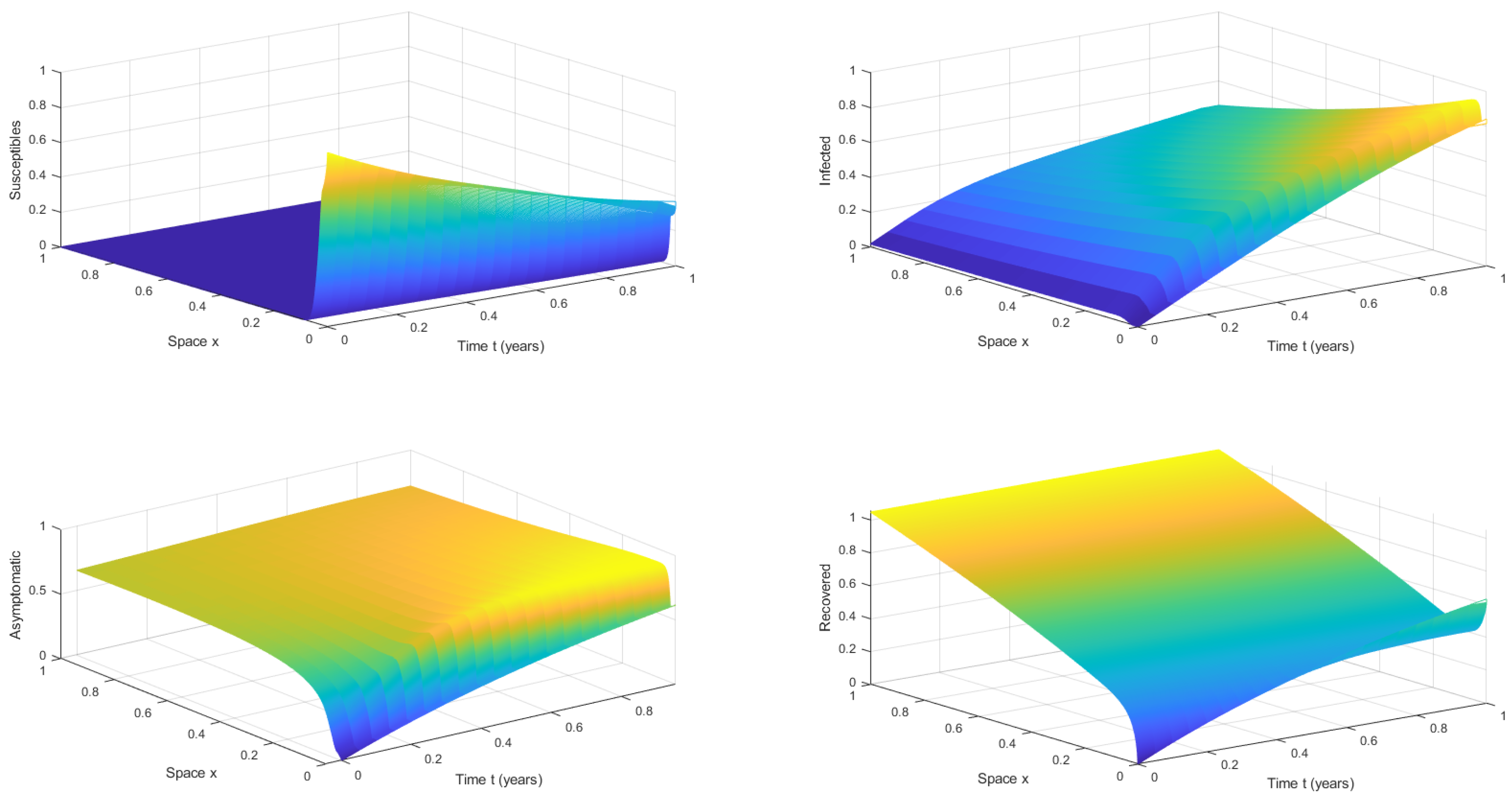
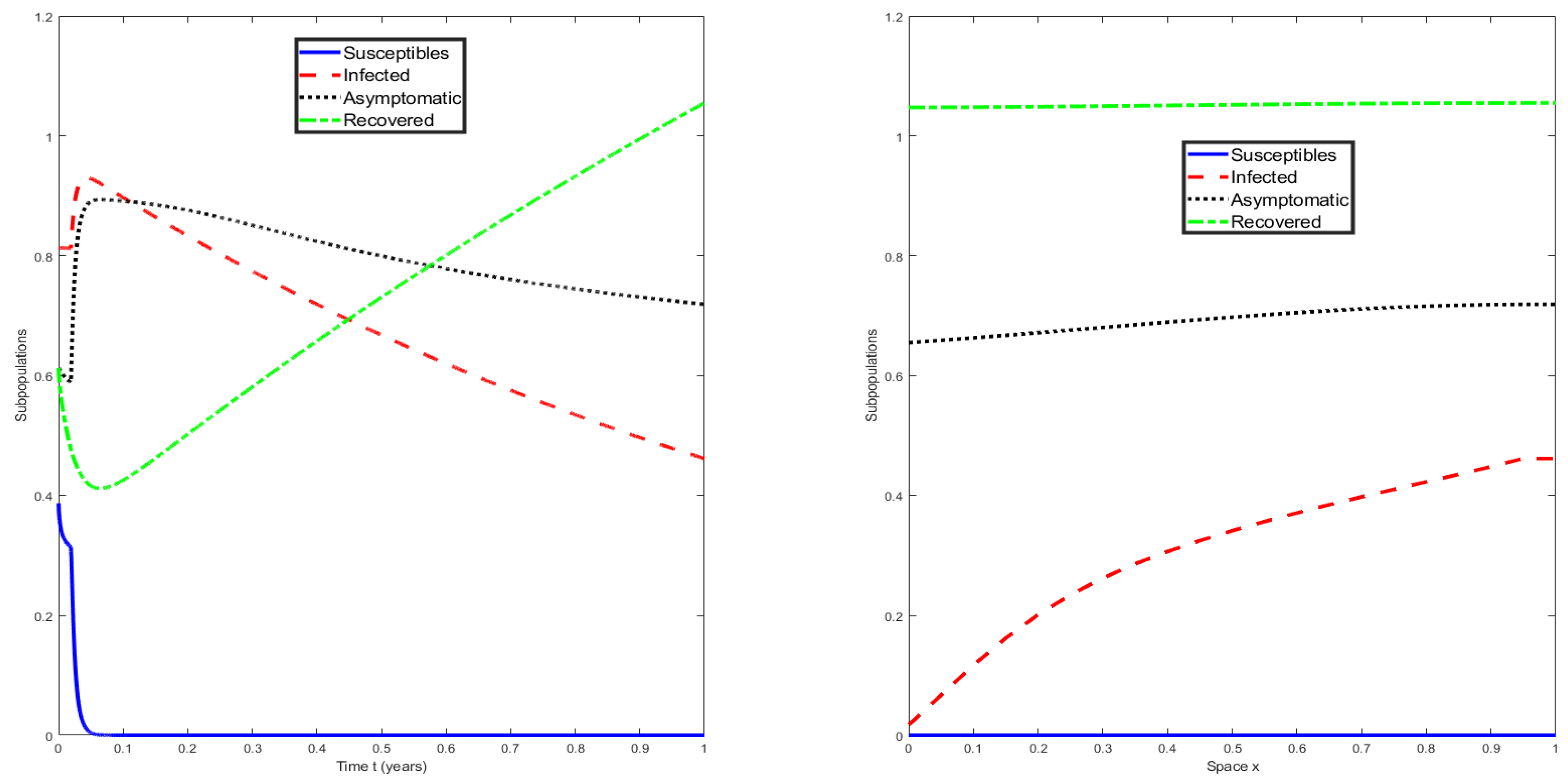
5. Numerical Simulations of the Mathematical Model

In this section, we present numerical simulations of the mathematical model (1), which is based on a system of partial differential equations with a discrete-time delay $\tau$. The numerical simulations allow us to examine the dynamics of a simplified scenario of the COVID-19 pandemic. In addition, they allow us to support the theoretical findings obtained in the previous subsections.

For the numerical simulations, we used available approximated real data where possible to test the theoretical results. Some parameter values are not known in the scientific literature, making it extremely difficult to find accurate values. There are many scientific works devoted to dealing with uncertainties in mathematical models for the COVID-19 pandemic and other epidemics. In addition, there are specific works devoted to the uncertainties associated with some parameter values. For instance, in [37,38,39,40,41], this topic is investigated as one of the main aims. In our work, one of the main aims was the mathematical analysis of the model (1). Nevertheless, we used approximated realistic values for most of the parameters. In particular, we used approximated initial conditions from the early phase of the COVID-19 pandemic in Colombia. For the history functions, we assumed constant values while accounting for proportions in the early phase of the COVID-19 situation in Colombia. This is a common approach used in similar theoretical works that deal with discrete-time delays. The time delay, which takes into account the incubation time, was set at seven days, which is slightly longer than in other works but still plausible. For asymptomatic cases, we assumed that 30% of cases were asymptomatic, which is one of the scenarios assumed by the CDC. For the transmission rate, we chose a parameter value (beta) that allows us to verify the theoretical results and also aligns with reported basic reproduction numbers from other studies.

We simulated a specific scenario where ${\mathcal{R}}_0>1$. Based on the theoretical results, COVID-19 did not become extinct. We present the numerical simulations, where the dynamics of the model (1) can be observed in space and time. The main idea behind this simulation is to use a specific value of the basic reproduction number ${\mathcal{R}}_0$ since this threshold parameter is crucial for the dynamics of the disease. The simulations provide further insights, such as the transient and long-term behavior of the disease for a specific simplified scenario.

We executed the simulations using the IMEX method [42]. This method combines the explicit and implicit Euler methods. In addition, we relied on the ghost-node technique to discretize the model (1) [43,44]. The numerical simulations were implemented using Matlab version R2023a. These simulations allow us to illustrate and support the theoretical results. The general basic idea of the numerical method is to divide the domain $[0,L]\times [0,T]$ using a grid of points. The space-step size is given by $h=\frac{L}{n}$ and the time-step size is given by $k=\frac{T}{m}$ for $m,n\in \mathbb{N}$. In addition, the value of k was chosen such that $\tau =pk$ for some integer number p such that $p\ge 1$.

For the numerical simulations, we used some illustrative numerical values for the parameters of the mathematical model (1). These values were as follows: $\mathsf{\Lambda }=(180\times 365)/50352943$, $\mu =0.0001523835\ast 365$, $\eta =0.00006586199\times 365$, $\beta =0.4\times 365$, $\alpha =0.65$, $r=0.3$, ${\nu }_S=3.75+{10}^{-5}\times 365,{\nu }_I=0.75\times {10}^{-10}\times 365,{\nu }_A=0.75\times {10}^{-3}\times 365$, and ${\nu }_R=3.75+{10}^{-5}\times 365$. For the domain, we used $[0,1]\times [0,T]$, where T is the simulation time. The initial conditions, that is, the history functions, were assumed to be constant and given by $S(x,0)=46054839/50352943$, $A(x,0)=35005/50352943$, $I(x,0)=10500/50352943$, and $R(x,0)=4160000/50352943$ for $\theta \in [-\tau ,0]$. The boundary conditions were Neumann-type, as explained in the previous section. Figure 2 shows the numerical solution of the mathematical model (1) with a discrete-time delay $\tau =7/365$ and ${\mathcal{R}}_0=1.27>1$ for $t\in [0,1]$. It can be seen that the susceptible population $S(x,t)$ becomes extinct, whereas the infected $I(x,t)$ and asymptomatic $A(x,t)$ populations are approaching an endemic steady state through traveling waves. On the left-hand side of Figure 3, we can see the numerical solution of the mathematical model (1) at $x=1$. Again, it can be observed that the susceptible population becomes extinct, whereas the infected and asymptomatic populations are approaching an endemic steady state, as expected. On the right-hand side of Figure 3, we can see the numerical solution of the mathematical model (1) at the final time of $t=1$ for different values of x. It can be seen that the disease is approaching an endemic equilibrium state since ${\mathcal{R}}_0=1.27>1$. This numerical result supports the theoretical results, despite the fact that the model (1) was designed for the early phase of the COVID-19 pandemic. A more complex model is needed for the current pandemic to account for vaccinated individuals and the waning of immunity [8,45,46,47].

Figure 2. Numerical solution of the mathematical model (1) with a discrete-time delay $\tau =7/365$, $t\in [0,1]$, and ${\mathcal{R}}_0=1.27>1$.

Figure 3. Numerical solution of the mathematical model (1) at $t=1$ with a discrete-time delay $\tau =7/365$, $t=1$, and ${\mathcal{R}}_0=1.27>1$.

6. Conclusions

In this article, we studied the existence of traveling waves in a diffusive mathematical model representing the transmission of a virus within a population composed of susceptible $\left(S\right),$ infected $\left(I\right),$ asymptomatic $\left(A\right)$, and recovered $\left(R\right)$ individuals. The constructed model is a simplification of a complex real-world situation, but it provides further insight into the dynamics of different diseases, such as COVID-19. Furthermore, it demonstrates a mathematical modeling approach that considers spatial effects and time delays in the biological process related to SARS-CoV-2 virus transmission among the human population. An analytical study was performed, where the existence of solutions of traveling waves within a bounded domain was demonstrated using the upper and lower coupled solutions method. The existence and local asymptotic stability of both endemic ($E_e$) and disease-free $\left(E_0\right)$ equilibrium states were also determined. We presented numerical simulations of the solutions in order to provide additional support to the theoretical results. In addition, we provided further simulations in order to illustrate the effects of discrete-time delays on the dynamics of the traveling waves.

References

- Hethcote, H.W. Mathematics of infectious diseases. SIAM Rev. 2005, 42, 599–653. [Google Scholar] [CrossRef]
- Arino, J.; Van Den Driessche, P. Time delays in epidemic models. Delay Differ. Equ. Appl. Nato Sci. Ser. 2006, 205, 539–578. [Google Scholar]
- Brauer, F.; Castillo-Chavez, C. Mathematical Models for Communicable Diseases; SIAM: Philadelphia, PA, USA, 2012. [Google Scholar]
- Schiesser, W.E. Mathematical Modeling Approach to Infectious Diseases, A: Cross Diffusion Pde Models for Epidemiology; World Scientific: Singapore, 2018. [Google Scholar]
- Trejos, D.Y.; Valverde, J.C.; Venturino, E. Dynamics of infectious diseases: A review of the main biological aspects and their mathematical translation. Appl. Math. Nonlinear Sci. 2022, 7, 1–26. [Google Scholar] [CrossRef]
- Aràndiga, F.; Baeza, A.; Cordero-Carrión, I.; Donat, R.; Martí, M.C.; Mulet, P.; Yáñez, D.F. A spatial-temporal model for the evolution of the COVID-19 pandemic in Spain including mobility. Mathematics 2020, 8, 1677. [Google Scholar] [CrossRef]
- Agrawal, M.; Kanitkar, M.; Vidyasagar, M. Modelling the spread of SARS-CoV-2 pandemic-Impact of lockdowns and interventions. Indian J. Med. Res. 2021, 153, 175. [Google Scholar]
- González-Parra, G.; Arenas, A.J. Mathematical Modeling of SARS-CoV-2 Omicron Wave under Vaccination Effects. Computation 2023, 11, 36. [Google Scholar] [CrossRef]
- Görtz, M.; Krug, J. Nonlinear dynamics of an epidemic compartment model with asymptomatic infections and mitigation. J. Phys. Math. Theor. 2022, 55, 414005. [Google Scholar] [CrossRef]
- Goel, K.; Nilam. A nonlinear SAIR epidemic model: Effect of awareness class, nonlinear incidences, saturated treatment and time delay. Ric. Mat. 2022, 1–35. [Google Scholar] [CrossRef]
- Yang, J.; Liang, S.; Zhang, Y. Travelling waves of a delayed SIR epidemic model with nonlinear incidence rate and spatial diffusion. PLoS ONE 2011, 6, e21128. [Google Scholar] [CrossRef] [PubMed]
- Wu, J.; Zou, X. Traveling wave fronts of reaction-diffusion systems with delay. J. Dyn. Differ. Equ. 2001, 13, 651–687. [Google Scholar] [CrossRef]
- Tian, C.; Lin, Z. Traveling wave solutions for delayed reaction-diffusion systems. arXiv 2010, arXiv:1007.3429. [Google Scholar]
- Zou, X.; Wu, J. Existence of traveling wave fronts in delayed reaction-diffusion systems via the monotone iteration method. Proc. Am. Math. Soc. 1997, 125, 2589–2598. [Google Scholar] [CrossRef]
- Wu, X.; Tian, B.; Yuan, R. Traveling waves in an SEIR epidemic model with a general nonlinear incidence rate. Appl. Anal. 2020, 99, 133–157. [Google Scholar] [CrossRef]
- Wachira, C.; Lawi, G.; Omondi, L. Travelling Wave Analysis of a Diffusive COVID-19 Model. J. Appl. Math. 2022, 2022, 6052274. [Google Scholar] [CrossRef]
- Alaoui, A.L.; Ammi, M.R.S.; Tilioua, M.; Torres, D.F. Global stability of a diffusive SEIR epidemic model with distributed delay. In Mathematical Analysis of Infectious Diseases; Elsevier: Amsterdam, The Netherlands, 2022; pp. 191–209. [Google Scholar]
- Ma, Y.; Cui, Y.; Wang, M. Global stability and control strategies of a SIQRS epidemic model with time delay. Math. Methods Appl. Sci. 2022, 45, 8269–8293. [Google Scholar] [CrossRef]
- Samanta, G.; Sen, P.; Maiti, A. A delayed epidemic model of diseases through droplet infection and direct contact with saturation incidence and pulse vaccination. Syst. Sci. Control. Eng. 2016, 4, 320–333. [Google Scholar] [CrossRef]
- Sultana, S.; González-Parra, G.; Arenas, A.J. Dynamics of toxoplasmosis in the cat’s population with an exposed stage and a time delay. Math. Biosci. Eng. 2022, 19, 12655–12676. [Google Scholar] [CrossRef] [PubMed]
- Tchuenche, J.M.; Nwagwo, A. Local stability of an SIR epidemic model and effect of time delay. Math. Methods Appl. Sci. 2009, 32, 2160–2175. [Google Scholar] [CrossRef]
- Gutiérrez-Jara, J.P.; Vogt-Geisse, K.; Cabrera, M.; Córdova-Lepe, F.; Muñoz-Quezada, M.T. Effects of human mobility and behavior on disease transmission in a COVID-19 mathematical model. Sci. Rep. 2022, 12, 10840. [Google Scholar] [CrossRef] [PubMed]
- Kevrekidis, P.G.; Cuevas-Maraver, J.; Drossinos, Y.; Rapti, Z.; Kevrekidis, G.A. Reaction-diffusion spatial modeling of COVID-19: Greece and Andalusia as case examples. Phys. Rev. E 2021, 104, 024412. [Google Scholar] [CrossRef] [PubMed]
- Beretta, E.; Takeuchi, Y. Global stability of an SIR epidemic model with time delays. J. Math. Biol. 1995, 33, 250–260. [Google Scholar] [CrossRef]
- Chen-Charpentier, B. Delays and Exposed Populations in Infection Models. Mathematics 2023, 11, 1919. [Google Scholar] [CrossRef]
- Kuang, Y. Delay Differential Equations: With Applications in Population Dynamics; Academic Press: Cambridge, MA, USA, 1993. [Google Scholar]
- Ma, W.; Song, M.; Takeuchi, Y. Global stability of an SIR epidemicmodel with time delay. Appl. Math. Lett. 2004, 17, 1141–1145. [Google Scholar] [CrossRef]
- Nastasi, G.; Perrone, C.; Taffara, S.; Vitanza, G. A time-delayed deterministic model for the spread of COVID-19 with calibration on a real dataset. Mathematics 2022, 10, 661. [Google Scholar] [CrossRef]
- Zaman, G.; Kang, Y.H.; Jung, I.H. Optimal treatment of an SIR epidemic model with time delay. BioSystems 2009, 98, 43–50. [Google Scholar] [CrossRef] [PubMed]
- Li, J.; Sun, G.Q.; Jin, Z. Pattern formation of an epidemic model with time delay. Phys. A Stat. Mech. Its Appl. 2014, 403, 100–109. [Google Scholar] [CrossRef]
- Gan, Q.; Xu, R.; Yang, P. Travelling waves of a delayed SIRS epidemic model with spatial diffusion. Nonlinear Anal. Real World Appl. 2011, 12, 52–68. [Google Scholar] [CrossRef]
- Smith, H. An Introduction to Delay Differential Equations with Applications to the Life Sciences; Springer: Berlin/Heidelberg, Germany, 2011. [Google Scholar]
- Viguerie, A.; Lorenzo, G.; Auricchio, F.; Baroli, D.; Hughes, T.J.; Patton, A.; Reali, A.; Yankeelov, T.E.; Veneziani, A. Simulating the spread of COVID-19 via a spatially-resolved susceptible-exposed-infected-recovered-deceased (SEIRD) model with heterogeneous diffusion. Appl. Math. Lett. 2021, 111, 106617. [Google Scholar] [CrossRef] [PubMed]
- Lin, Z.; Pedersen, M.; Tian, C. Traveling wave solutions for reaction-diffusion systems. Nonlinear Anal. Theory Methods Appl. 2010, 73, 3303–3313. [Google Scholar] [CrossRef]
- Hernández, E.; Trofimchuk, S. Nonstandard quasi-monotonicity: An application to the wave existence in a neutral KPP-Fisher equation. J. Dyn. Differ. Equ. 2020, 32, 921–939. [Google Scholar] [CrossRef]
- Brauer, F. Absolute stability in delay equations. J. Differ. Equ. 1987, 69, 185–191. [Google Scholar] [CrossRef]
- Armstrong, E.; Runge, M.; Gerardin, J. Identifying the measurements required to estimate rates of COVID-19 transmission, infection, and detection, using variational data assimilation. Infect. Dis. Model. 2021, 6, 133–147. [Google Scholar] [CrossRef]
- Bastos, S.B.; Morato, M.M.; Cajueiro, D.O.; Normey-Rico, J.E. The COVID-19 (SARS-CoV-2) uncertainty tripod in Brazil: Assessments on model-based predictions with large under-reporting. Alex. Eng. J. 2021, 60, 4363–4380. [Google Scholar] [CrossRef]
- Libotte, G.B.; Dos Anjos, L.; Almeida, R.C.; Malta, S.M.; Silva, R.S. Framework for enhancing the estimation of model parameters for data with a high level of uncertainty. Nonlinear Dyn. 2022, 107, 1919–1936. [Google Scholar] [CrossRef] [PubMed]
- Olivares, A.; Staffetti, E. Uncertainty quantification of a mathematical model of COVID-19 transmission dynamics with mass vaccination strategy. Chaos Solitons Fractals 2021, 146, 110895. [Google Scholar] [CrossRef] [PubMed]
- Sanchez-Daza, A.; Medina-Ortiz, D.; Olivera-Nappa, A.; Contreras, S. COVID-19 modeling under uncertainty: Statistical data analysis for unveiling true spreading dynamics and guiding correct epidemiological management. In Modeling, Control and Drug Development for COVID-19 Outbreak Prevention; Springer: Berlin/Heidelberg, Germany, 2022; pp. 245–282. [Google Scholar]
- Yau, M.A. Analysis of Spatial Dynamics and Time Delays in Epidemic Models. Ph.D. Thesis, University of Sussex, Brighton, UK, 2014. [Google Scholar]
- Angstmann, C.N.; Henry, B.I.; Jacobs, B.A.; McGann, A.V. Numeric solution of advection-diffusion equations by a discrete time random walk scheme. Numer. Methods Partial. Differ. Equ. 2020, 36, 680–704. [Google Scholar] [CrossRef]
- Yang, C.; Sun, T. Crank-Nicolson finite difference schemes for parabolic optimal Dirichlet boundary control problems. Math. Methods Appl. Sci. 2022, 45, 7346–7363. [Google Scholar] [CrossRef]
- Calvetti, D.; Somersalo, E. Post-pandemic modeling of COVID-19: Waning immunity determines recurrence frequency. Math. Biosci. 2023, 365, 109067. [Google Scholar] [CrossRef] [PubMed]
- Luebben, G.; González-Parra, G.; Cervantes, B. Study of optimal vaccination strategies for early COVID-19 pandemic using an age-structured mathematical model: A case study of the USA. Math. Biosci. Eng. 2023, 20, 10828–10865. [Google Scholar] [CrossRef] [PubMed]
- Viguerie, A.; Carletti, M.; Silvestri, G.; Veneziani, A. Mathematical Modeling of Periodic Outbreaks with Waning Immunity: A Possible Long-Term Description of COVID-19. Mathematics 2023, 11, 4918. [Google Scholar] [CrossRef]
- Yu, Z.X.; Yuan, R. Traveling waves of delayed reaction-diffusion systems with applications. Nonlinear Anal. Real World Appl. 2011, 12, 2475–2488. [Google Scholar] [CrossRef]
- Rudin, W. Principles of Mathematical Analysis; McGraw-Hill: New York, NY, USA, 1953; Volume 3. [Google Scholar]
- Zeidler, E.; Wadsack, P.R. Nonlinear Functional Analysis and Its Applications: Fixed-Point Theorems; Wadsack, P.R., Translator; Springer: Berlin/Heidelberg, Germany, 1993. [Google Scholar]
Disclaimer/Publisher’s Note: The statements, opinions and data contained in all publications are solely those of the individual author(s) and contributor(s) and not of MDPI and/or the editor(s). MDPI and/or the editor(s) disclaim responsibility for any injury to people or property resulting from any ideas, methods, instructions or products referred to in the content. |
© 2024 by the authors. Licensee MDPI, Basel, Switzerland. This article is an open access article distributed under the terms and conditions of the Creative Commons Attribution (CC BY) license (https://creativecommons.org/licenses/by/4.0/).