Abstract
The answer to the question posed in the title is yes if the context (the list of variables defining the motion control problem) is dimensionally similar. This article explores the use of the Buckingham theorem as a tool to encode the control policies of physical systems into a more generic form of knowledge that can be reused in various situations. This approach can be interpreted as enforcing invariance to the scaling of the fundamental units in an algorithm learning a control policy. First, we show, by restating the solution to a motion control problem using dimensionless variables, that (1) the policy mapping involves a reduced number of parameters and (2) control policies generated numerically for a specific system can be transferred exactly to a subset of dimensionally similar systems by scaling the input and output variables appropriately. Those two generic theoretical results are then demonstrated, with numerically generated optimal controllers, for the classic motion control problem of swinging up a torque-limited inverted pendulum and positioning a vehicle in slippery conditions. We also discuss the concept of regime, a region in the space of context variables, that can help to relax the similarity condition. Furthermore, we discuss how applying dimensional scaling of the input and output of a context-specific black-box policy is equivalent to substituting new system parameters in an analytical equation under some conditions, using a linear quadratic regulator (LQR) and a computed torque controller as examples. It remains to be seen how practical this approach can be to generalize policies for more complex high-dimensional problems, but the early results show that it is a promising transfer learning tool for numerical approaches like dynamic programming and reinforcement learning.
Keywords:
optimal control; dimensional analysis; transfer learning; reinforcement learning; motion control; dynamics; physics-informed learning MSC:
70Q05; 00A73; 93C85; 68T40
1. Introduction
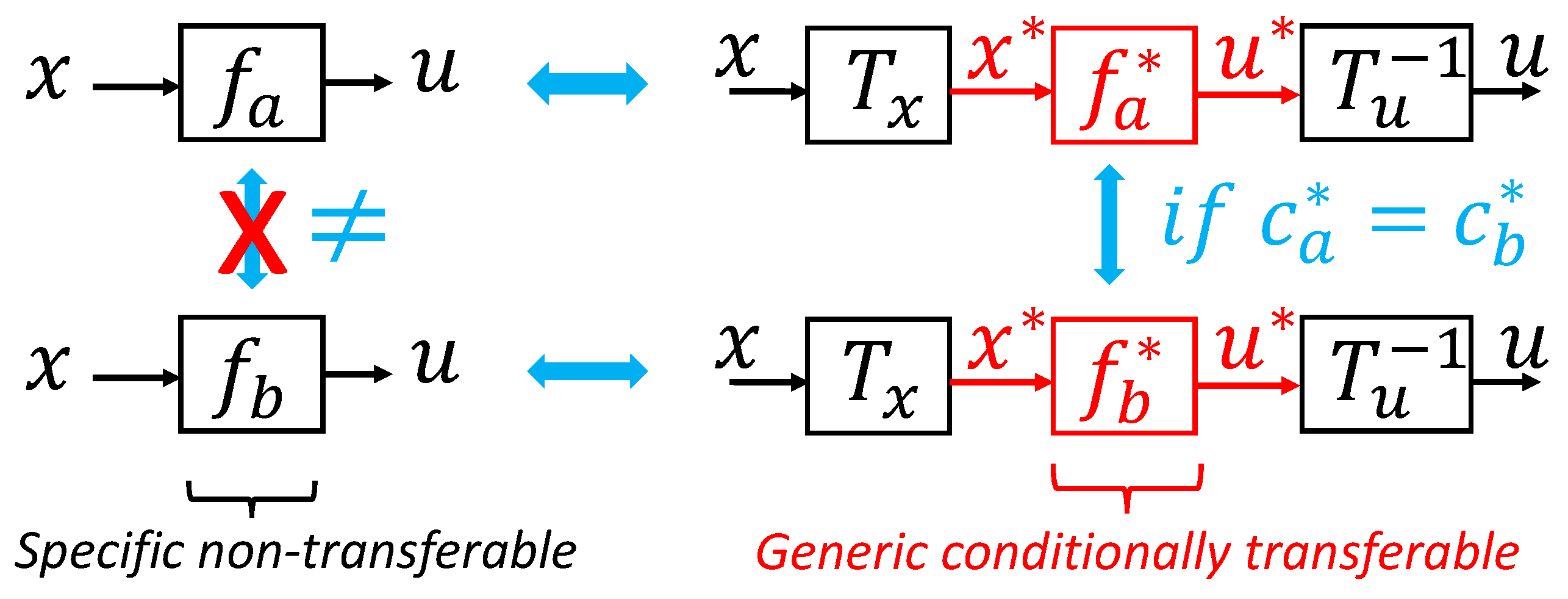
To solve challenging motion control problems in robotics (locomotion, manipulation, vehicle control, etc.), many approaches now include a type of mathematical optimization that has no closed-form solution and that is solved numerically, either online (trajectory optimization [1], model predictive control [2], etc.) or offline (reinforcement learning [3]). Numerical tools, however, have a major drawback compared to simpler analytical approaches: the parameters of the problem do not appear explicitly in the solutions, which makes it much harder to generalize and reuse the results. Analytical solutions to control problems have the useful property of allowing the solution to be adjusted to different system parameters by simply substituting the new values in the equation. For instance, an analytical feedback law solution to a robot motion control problem can be transferred to a similar system by adjusting the values of the parameters (lengths, masses, etc.) in the equation. However, with a reinforcement learning solution, we would have to re-conduct all the training, implying (generally) multiple hours of data collection and/or computation. It would be a great asset to have the ability to adjust black-box numerical solutions with respect to some problem parameters.
In this paper, we explore the concept of dimensionless policies, a more generic form of knowledge conceptually illustrated in Figure 1, as an approach to generalize numerical solutions to motion control problems. First, in Section 2, we use dimensional analysis (i.e., the Buckingham theorem [4]) to show that motion control problems with dimensionally similar context variables must share the same feedback law solution when expressed in a dimensionless form, and discuss the implications. Two main generic theoretical results, relevant for any physically meaningful control policies, are presented as Theorems 1 and 2. Then, in Section 3, we present two case studies with numerical results. Optimal feedback laws computed with a dynamic programming algorithm are used to demonstrate the theoretical results and their relevance for (1) the classical motion control problem of swinging up an inverted pendulum in Section 3.1 and (2) a car motion control problem in Section 3.2. Furthermore, in Section 4, we illustrate—with two examples—how the proposed dimensional scaling is equivalent to changing parameters in an analytical solution.
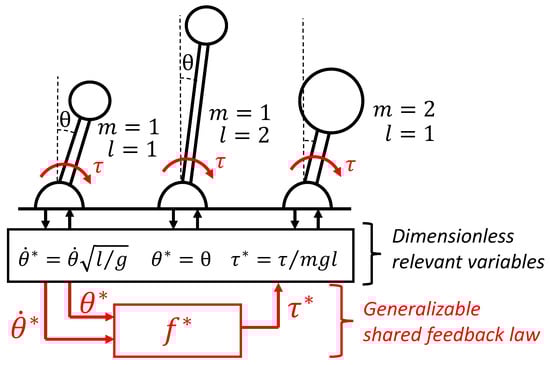
Figure 1.
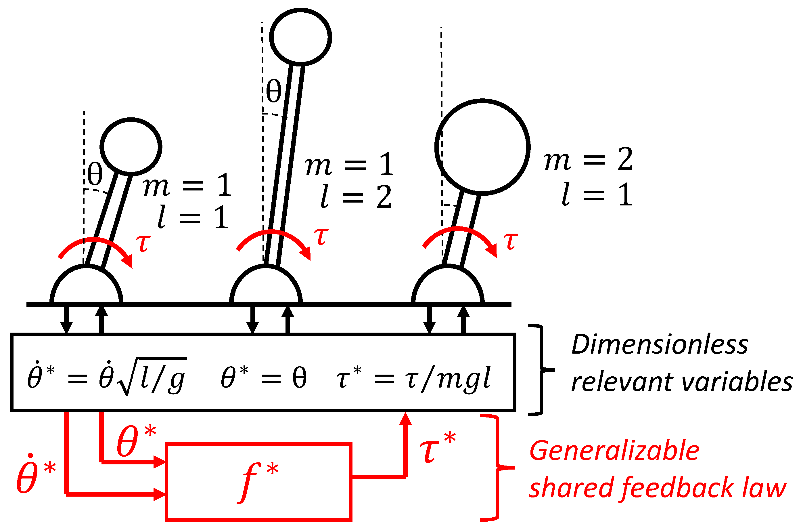
Shared dimensionless policy for inverted pendulums: under some conditions, various dynamic systems will share the same optimal policy up to scaling factors that can be found based on a dimensional analysis.
A very promising application of the concept of dimensionless policies is to empower reinforcement learning schemes, for which data efficiency is critical [5]. For instance, it would be interesting to use the data of all the vehicles on the road, even if they are of varying dimensions and dynamic characteristics, to learn appropriate maneuvers in situations that occur very rarely. This idea of reusing data or results in a different context is usually called transfer learning [6] and has received a great deal of research attention, mostly targeted at applying a learned policy to new tasks. The more specific idea of transferring policies and data between systems/robots has also been explored, with schemes based on modular blocks [7], invariant features [8], a dynamic map [9], a vector representation of each robot hardware [10], or using tools from adaptive control [11] and robust control [12]. Dimensionless numbers and dimensional analysis comprise a technique based on the idea that some relationships should not depend on units that can be used for analyzing many physical problems [4,13,14]. The most well-known application in the field of fluid mechanics is the idea of matching ratios (i.e., Reynolds, Prandtl, or Mach numbers) to allow for the generalization of experimental results between systems of various scales. The recent success of machine learning and data-driven schemes highlights the question of generalizing results, and there is renewed interest in using dimensional analysis in the context of learning [15,16,17]. In this paper, we present an initial exploration of how dimensional analysis can be applied specifically to help generalize policy solutions for motion control problems involving physically meaningful variables like force, length, mass, and time.
2. Dimensionless Policies
In the following section, we develop the concept of dimensionless policies based on the Buckingham theorem and present generic theoretical results that are relevant for any type of physically meaningful control policy.
2.1. Context Variables in the Policy Mapping
Here, we call a feedback law mapping f, specific to a given system, from a vector space representing the state x of the dynamic system to a vector space representing the control inputs u of the system:
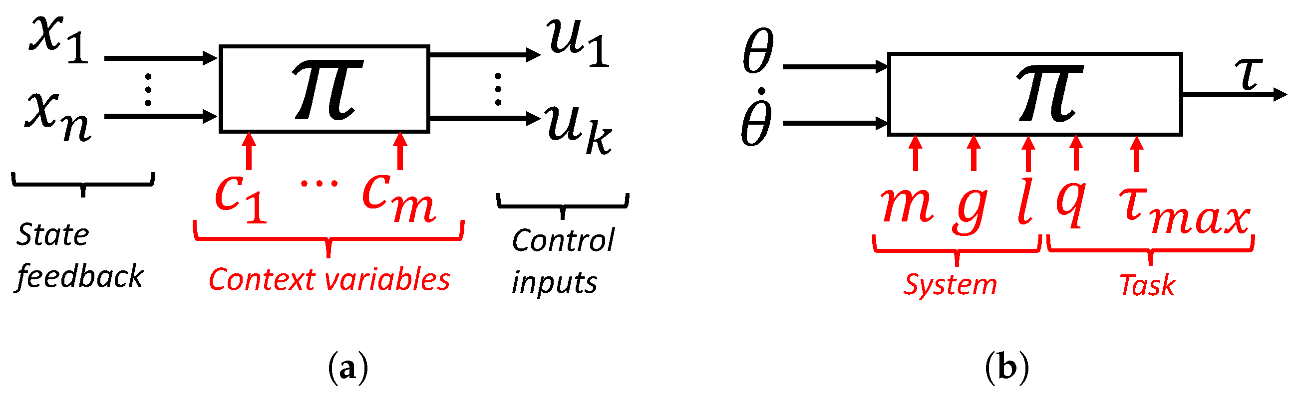
Under some assumptions (fully observable systems, additive costs, and infinite time horizon), the optimal feedback law is guaranteed to be in this state feedback form [18]. We will only consider motion control problems that lead to such time-independent feedback laws in the following analysis. To consider the question of how this system-specific feedback law can be transferred to a different context, it is useful to think about higher dimensional mapping , which is herein referred to as a policy, also having a vector of variables c describing the context as an additional input argument as illustrated in Figure 2.
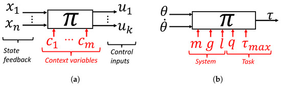
Figure 2.
The policy is a feedback law that also includes problem parameters as additional arguments. (a) Generic policy; (b) inverted pendulum example.
Definition 1.
A policy is defined as the solution to a motion control problem in the form of a function computing the control inputs u from the system states x and context parameters c as follows:
where k is the dimension of the control input vector, n is the dimension of the dynamic system state vector, and k is the dimension of the vector of context parameters.
The context c is a vector of relevant parameters defining the motion control problem, i.e., parameters that affect the feedback law solution. The policy is thus a mapping consisting of the feedback law solutions for all possible contexts. In Section 3.1, a case study is conducted by considering the optimal feedback law for swinging up a torque-limited inverted pendulum. For this example, the context variables are the pendulum mass m, the gravitational constant g, and the length l, as well as what we call task parameters: a weight parameter in the cost function q and a constraint on the maximum input torque. For a given pendulum state, the optimal torque is also a function of the context variables; i.e., the solution is different if the pendulum is heavier or more torque-limited.
Definition 2.
A feedback law with a subscript letter a is defined as the solution to a motion problem for a specific situation defined by an instance of context variables , as follows:
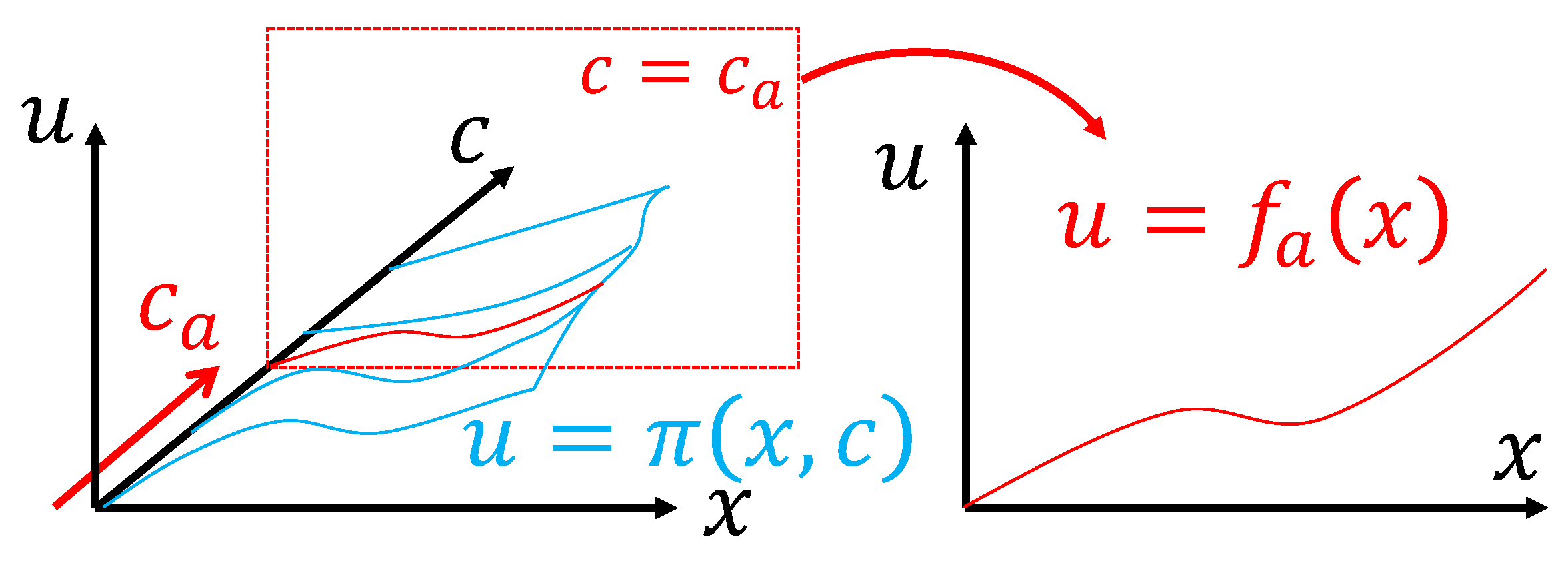
The feedback law thus represents a slice of the global policy when the context variables are fixed at values as illustrated in Figure 3.
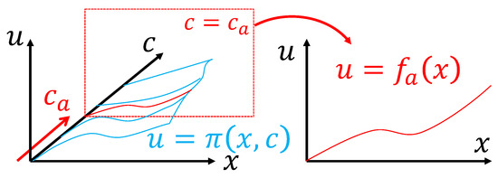
Figure 3.
A feedback law f is a slice of the higher dimensional policy mapping in a specific context.
The goal of generalizing a feedback law to a different context can thus be formulated into the following question: if a feedback law is known for a context described by variables , can this knowledge help us to deduce the policy solution in a different context, namely ?
Using the Buckingham theorem [4], we will show that, if the context is dimensionally similar, then both feedback laws must be equal up to scaling factors (Theorem 2).
2.2. Buckingham Theorem
The Buckingham theorem [4] is a tool based on dimensional analysis [13,14] that enables restating a relationship involving multiple physically meaningful dimensional variables using fewer dimensionless variables:
If d fundamental dimensions are involved in the n dimensional variables (for instance, time [T], length [L], and mass [M]), then the number of required dimensionless variables, often called groups, is . In most situations, the number of variables in the relationship can be reduced directly by the number of fundamental dimensions involved, and . The Buckingham theorem provides a methodology to generate the groups; however, the choice of groups is not unique. The approach is to select (arbitrarily) d variables involving the d fundamental dimensions independently, called the repeated variables. Then, the groups are generated by multiplying all the other variables by the repeated variables exponentiated by rational exponents selected to make the group dimensionless. Assuming , … , where the selected repeated variables, the groups are
Finding the correct exponents to make all groups dimensionless can be formulated as solving a linear system of d equations. We refer to previous literature for more details on the theorem, and here use it specifically on the defined concept of policy map.
2.3. Dimensional Analysis of the Policy Mapping
If a policy is physically meaningful (for example, a policy that computes a force based on position and velocity, but not a policy for playing chess), we can use the Buckingham theorem to simplify the policy in dimensionless form.
Theorem 1.
If a policy is physically meaningful and all its variables involve d fundamental dimensions that are independently present in the context variables c, then the policy can be restated in a dimensionless form as follows:
where the dimensionless variables can be related to dimensional variables using transformation matrices that depend only on the context variables as follows:
Furthermore, the transformation matrices can be used to relate the dimensional and dimensionless policy as follows:
Proof.
For a system with k control inputs, we can treat the policy as k mappings from states and context variables to each scalar control input :
where Equation (14) is the jth line of the policy in vector form, as described by Equation (2). Then, if the state vector is defined by n variables, and the context is defined by m (system and task) parameters, then each mapping is a relation between variables. Under the assumption that the policy involves physically meaningful variables, and that it is invariant under an arbitrary scaling of any fundamental dimensions—i.e., independent of a system of units—then we can apply the Buckingham theorem [4] to conclude that, if d dimensions are involved in all the variables, then Equation (14) can be restated as an equivalent relationship between p dimensionless groups where . Assuming that d dimensions are involved in the m context variables, and that we are in the typical scenario where maximum reduction is possible (), then we can select d context variables as the basis (the repeated variables) to scale all other variables into dimensionless groups. We denote dimensionless group as the base variables with an asterisk (*) as follows:
where exponents are rational numbers selected to make all equations dimensionless. We can then define transformation matrices and write Equations (15)–(17) in a vector form where the repeated variables are grouped into matrices defined as the following:
which correspond to Equations (10)–(12). Matrices and are square diagonal matrices and Equations (10) and (11) are thus inversibles (unless a repeated variable is equal to zero) and can be used to go back and forth between dimensional and dimensionless states and input variables. Matrix consists of a block of d columns of zeros, followed by a diagonal block of dimensions , and Equation (12) is not inversible. For a given context c, there is only one dimensionless context ; however, a given dimensionless context may correspond to multiple dimensional contexts c.
Then, the Buckingham theorem indicates that the relationship described by Equation (14) can be restated in a relationship between the groups involving d less variables, which, based on the selected repeated variable, corresponds to
By applying the same procedure to all control inputs, we can then assemble all k mappings back into a vector form, as follows:
corresponding to Equation (8). Finally, based on the defined transformations in Equations (10)–(12), we can relate the dimensional policy to the dimensionless version as follows:
which corresponds to Equation (13). □
2.4. Transferring Feedback Laws between Similar Systems
Based on the dimensional analysis, we can demonstrate that any feedback law can be generalized to a different context under the condition of dimensional similarity. In this section, we show that a feedback law can be transferred exactly to another motion control problem by scaling the input and output of the function based on matrices that can be computed using the dimensional analysis. The salient feature of this result is that the conditions are very generic; even a black-box discontinuous non-linear policy (such as those obtained using deep-reinforcement learning algorithms) can be transferred this way. The limitation is that the condition for an exact transfer is having equal dimensionless context variables .
First, it is useful to define dimensionless feedback laws that correspond to specific cases of the dimensionless policy, as we defined for the dimensional mapping.
Definition 3.
We denote a dimensionless feedback law , the global dimensionless policy for a specific instance of context variables , as follows:
where is the dimensionless version of the context variables instance , and equal to
Lemma 1.
Two feedback laws, which are solutions to the same motion control problem for two instances of context variables, will be equal in dimensionless form if they share the same dimensionless context:
Proof.
This follows from the definition:
□
Lemma 2.
In a specific context described by variables , a dimensional feedback law can be restated in dimensionless form, and vice versa, by scaling the input and the output using the defined transformation matrices and as follows:
Proof.
Starting from Equation (13) and substituting with a specific instance , then substituting policy maps on each side with feedback laws and based on the definition, we obtain Equation (30):
Then, starting from the right side of Equation (31) and substituting the function with Equation (30), the matrices are reduced to identity matrices and we obtain Equation (31):
□
Theorem 2.
If a feedback law is known—for instance, as the result of a numerical algorithm—and this is the solution to a motion control problem with context variables , we can compute the solution to the same motion control problem for different context variables by scaling the input and output of as follows:
if contexts and are dimensionally similar, i.e., if the following condition is true:
Proof.
First, can be written based on its dimensionless form in a context using Equation (30) from Lemma 2. Also, based on Lemma 1, under the similarity condition—i.e., or equivalently — we have that is equal to . Finally, can be written based on its dimensional form in a context , using Equation (31) from Lemma 2, as follows:
□
The idea is summarized in Figure 4. To transfer a feedback law, we must first extract the dimensionless form, a more generic form of knowledge, and then scale it back to the new context.

Figure 4.
Isolating the dimensionless knowledge in a policy enables its exact transfer to any dimensionally similar motion control problem.
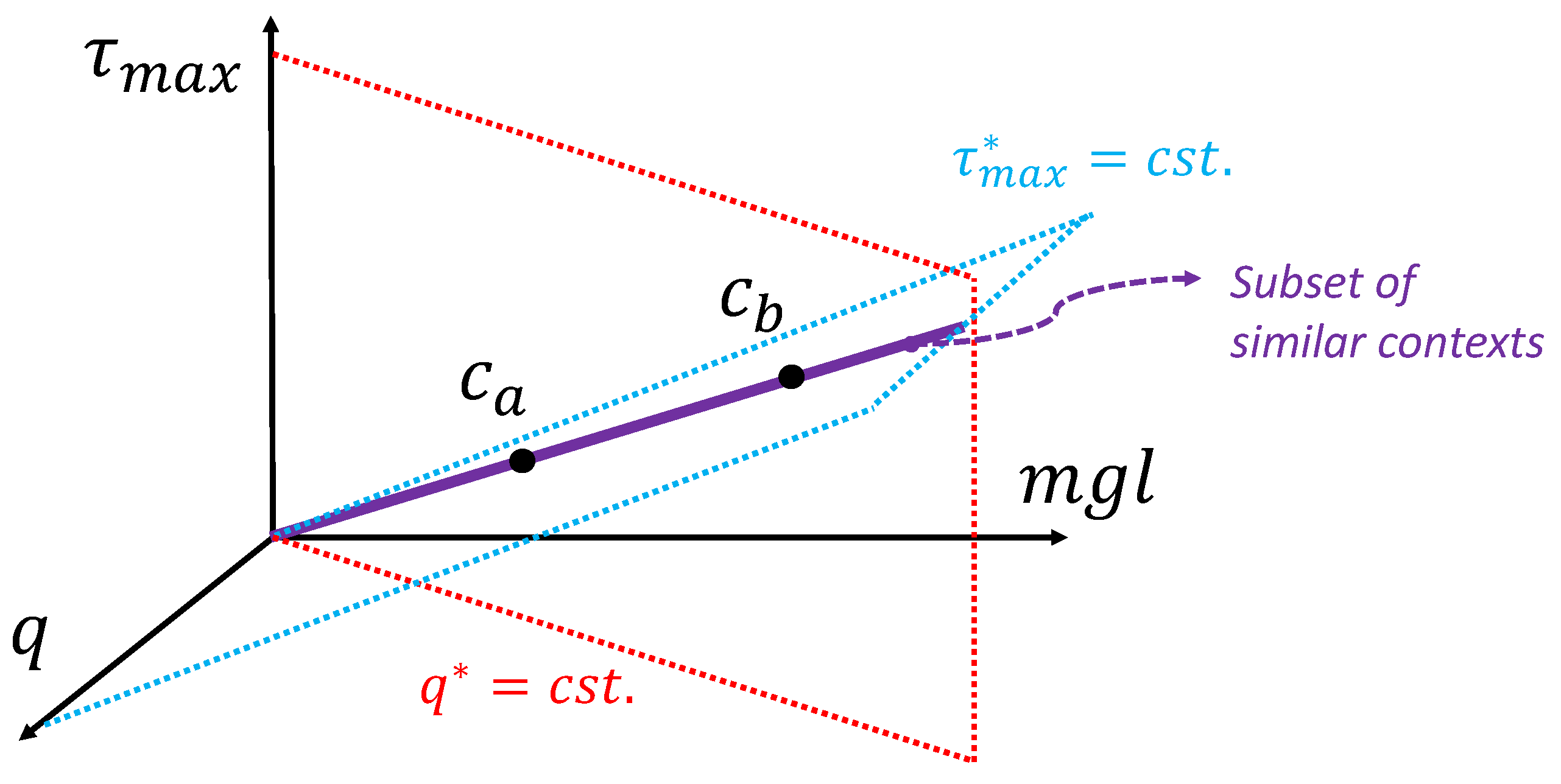
2.5. Dimensionally Similar Contexts
Equation (36) can be used to scale a policy for an exact transfer of policy solutions regarding context c sharing the same dimensionless context , a condition that is referred to as dimensionally similar. Equation (12) is a mapping from an m dimensional space to an dimensional space, and its inverse has multiple solutions. A given dimensionless context corresponds to a subset of all possible values of dimensional context c. As illustrated in Figure 5 and Figure 6 with low-dimensional examples ( and ), the subsets of context c leading to the same can be linear if is just a ratio of two variables of the same dimensions, or a non-linear curve if involves exponents leading to a more complex polynomial relationship. In general, when the context c involves many dimensions, it is important to note that the similarity condition means meeting multiple conditions (one for each element of the vector ) in a higher dimensional space, as illustrated in Figure 7 for the pendulum swing-up example that is studied in the next section. To some degree, this dimensionally similar context condition is a technique to regroup the motion control problems that are the same up to scaling factors. Therefore, it is also logical that their solutions should be equivalent up to scaling factors.
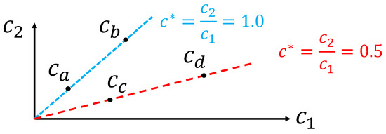
Figure 5.
Example of dimensionally similar context subsets that are lines in a plane ( and ). Context is dimensionally similar to but not to or .
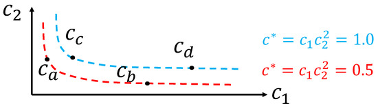
Figure 6.
Example of dimensionally similar context subsets that are non-linear curves in a plane ( and ). Context is dimensionally similar to but not to or .

Figure 7.
A dimensionally similar subset (equal ) can be represented as a line in a 3D space for the pendulum swing-up problem. The feedback law solutions to problem with context variables on the same line are equivalent in dimensionless form.
2.6. Summary of the Theoretical Results
The dimensional analysis leads us to the following relevant theoretical results, which are very generic since no assumptions on the form of the policy function are necessary:
- The global problem of learning , i.e., the feedback policies for all possible contexts, is simplified in a dimensionless form because we can remove d input dimensions from the unknown mapping (typically, d would be 2 or 3 for controlling a physical system involving time, force, and length); see Theorem 1.
- The feedback law solutions of dimensionally similar subset of contexts share the exact same solution when restated in a dimensionless form; see Lemma 1.
- A feedback law, which is a solution to a motion control problem in a context, can be transferred exactly to another context, under a condition of dimensional similarity, by appropriately scaling its inputs and outputs; see Theorem 2.
Just for illustration purposes, let us imagine we have a policy for a spherical submarine where the context is defined by a velocity, a viscosity, and a radius. In dimensionless form, we would find that the context can be described by a single variable, the Reynolds number, and that (1) learning the policy will be easier in dimensionless form because it is a function of a lesser number of variables and (2) if we know the feedback law solution for a specific context of velocity, viscosity, and radius, then we can actually re-use it for multiple versions of the same motion control problem sharing the same Reynolds number.
3. Case Studies with Numerical Results
In this section, we use numerically generated optimal policy solutions for two motion control problems as examples illustrating the salient features of the presented theoretical results of Section 2 and the potential for transfer learning.
3.1. Optimal Pendulum Swing-Up Task
The first numerical example is the classical pendulum swing-up task. This example illustrates that an optimal feedback law in the form of a table look-up generated for a pendulum of a given mass and length can be transferred to a pendulum of a different mass and length if the motion control problem is dimensionally similar. The example is also used to introduce the concept of regime for motion control problems.
3.1.1. Motion Control Problem
The motion control problem is defined here as finding a feedback law for controlling the dynamic system described by the following differential equation:
which minimizes the infinite horizon quadratic cost function provided by
subject to input constraints provided by
Note that, here, (1) the cost function parameter q has a power of two to allow its value to be in units of torque; (2) it was chosen not to penalize high velocity values for simplicity; (3) the weight multiplying the torque is set to one without a loss of generality as only the relative values of weights impact the optimal solution; and (4) all parameters are time-independent constants. Thus, assuming that there are no hidden variables and that Equations (41)–(43) fully describe the problem, the solution—i.e., the optimal policy for all contexts—involves the variables listed in Table 1, and should be of the form provided by

Table 1.
Pendulum swing-up optimal policy variables.
It is interesting to note that, while there are three system parameters, m, g, and l, they only appear independently in two groups in the dynamic equation. We can thus consider only two system parameters. For convenience, we selected , corresponding to the maximum static gravitational torque (i.e., when the pendulum is horizontal), and the natural frequency , as listed in Table 2.
Table 2.
Pendulum reduced system parameters.
3.1.2. Dimensional Analysis
Here, we have one control input, two states, two system parameters, and two task parameters, for a total of variables involved. In those variables, only independent dimensions ( and ) are present. Using and as the repeated variables leads to the following dimensionless groups:
All three torque variables (, q, and ) are scaled by the maximum gravitational torque, and the pendulum velocity variable is scaled by the natural pendulum frequency. The transformation matrices are thus
By applying the Buckingham theorem [4], Equation (44) can be restated as a relationship between the five dimensionless groups:
According to the results of Section 2, for dimensionally similar swing-up contexts (meaning those with equal and ratios), the optimal feedback laws should be equivalent in their dimensionless forms. In other words, the optimal policy , found in the specific context , and the optimal policy , in a second context, , are equal when restated in dimensionless form: if and . Furthermore, can be obtained from or vice versa using the scaling formula provided by Equation (36) if this condition is met. However, if or , then cannot provide us with information on without additional assumptions. Figure 7 illustrates that, for the pendulum swing-up problem, the similarity condition can be represented as a line in a three-dimensional space created by three dimensional context variables. Each condition of equal values of and is a plane in this space, and the intersection of the two planes is the subset of context meeting the two conditions. Also, it is interesting to note that the fourth context variable is not an additional axis here because it is not involved in Equation (52).
3.1.3. Numerical Results
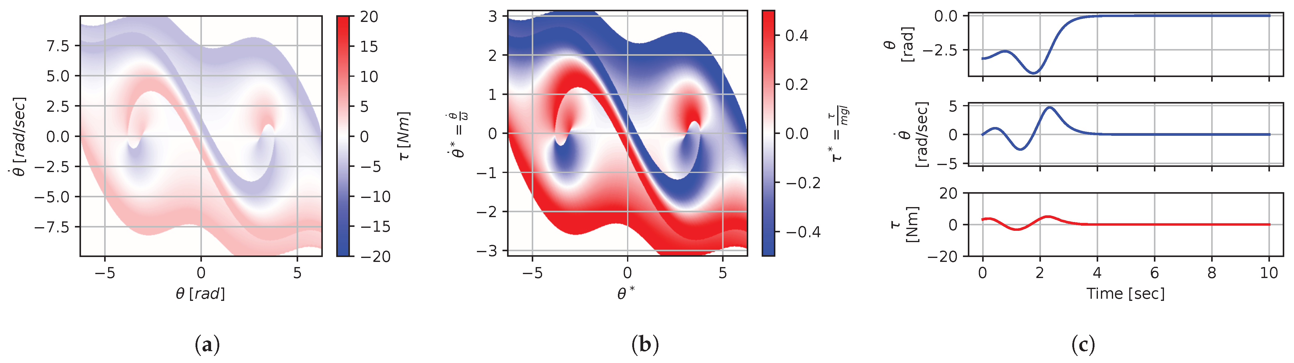
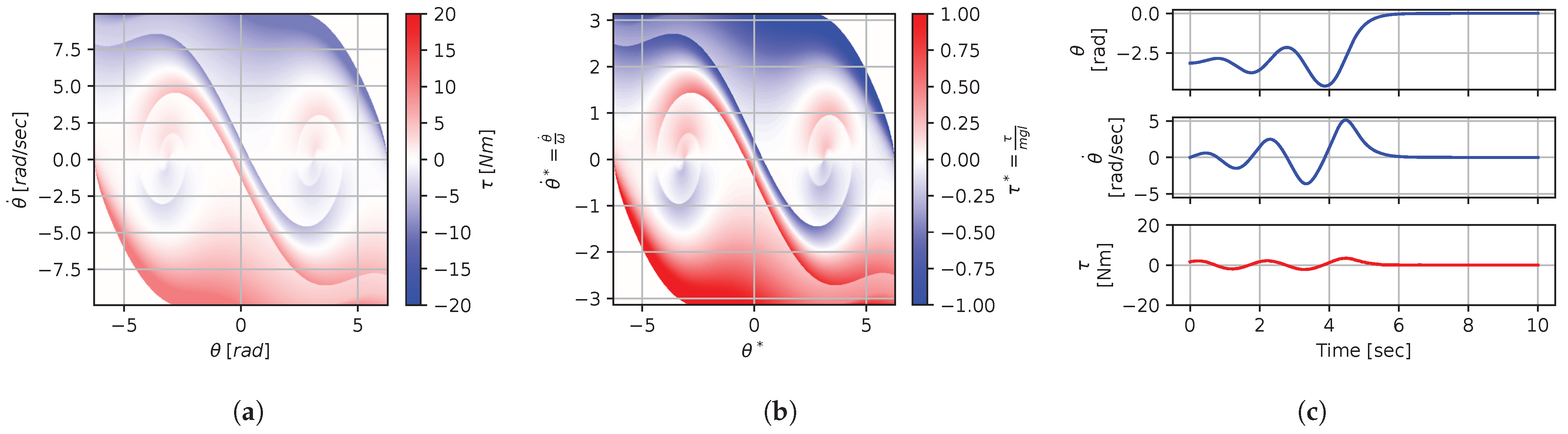
Here, we use a numerical algorithm (methodological details are presented in Section 3.1.5) to compute numerical solutions to the motion control problem defined by Equations (41)–(43). The algorithm computes feedback laws in the form of look-up tables, based on a discretized grid of the state space. The optimal (up to discretization errors) feedback laws are computed for nine instances of context variables, which are listed in Table 3. In those nine contexts, there are three subsets of three dimensionally similar contexts. Also, each subset includes the same three pendulums: a regular pendulum, one that is two times longer, and one that is twice as heavy (as illustrated in Figure 1). Contexts , , and describe a task where the torque is limited to half the maximum gravitational torque. Contexts , , and describe a task where the application of large torques is highly penalized by the cost function. Contexts , , and describe a task where position errors are highly penalized by the cost function.
Table 3.
Pendulum swing-up problem context variables.
Figure 8, Figure 9, Figure 10, Figure 11, Figure 12, Figure 13, Figure 14, Figure 15 and Figure 16 illustrate that, for each subset with equal dimensionless context, the dimensional feedback laws generated look numerically very similar. They are similar up to the scaling of their axis, if we neglect slight differences due to discretization errors. Furthermore, the figures also illustrate that the dimensionless version of the feedback laws (), computed using Equation (31), is equal within each dimensionally similar subset. These were the expected results predicted by the dimensional analysis presented in Section 2.

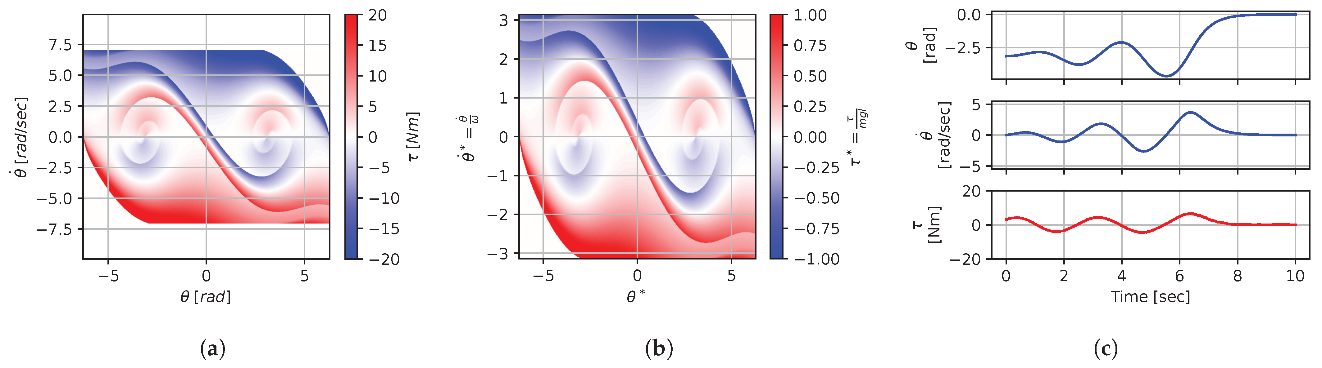
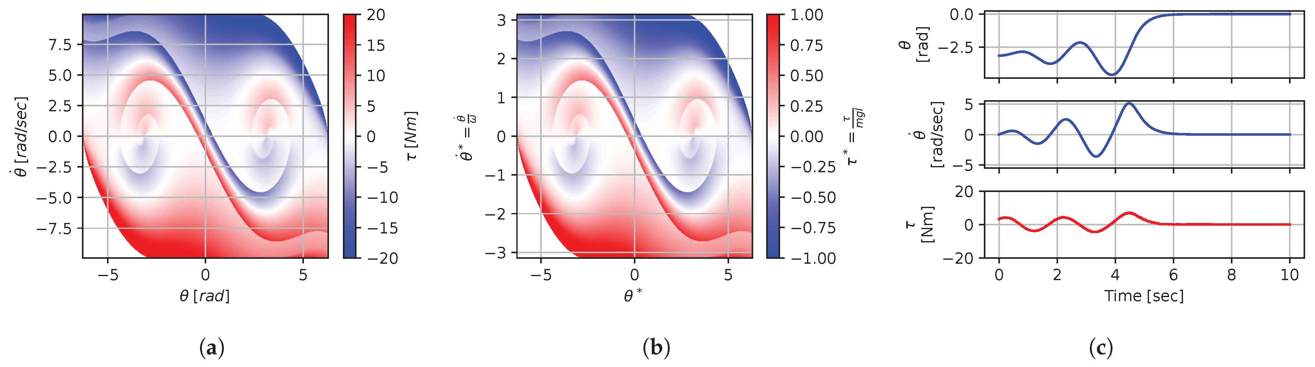
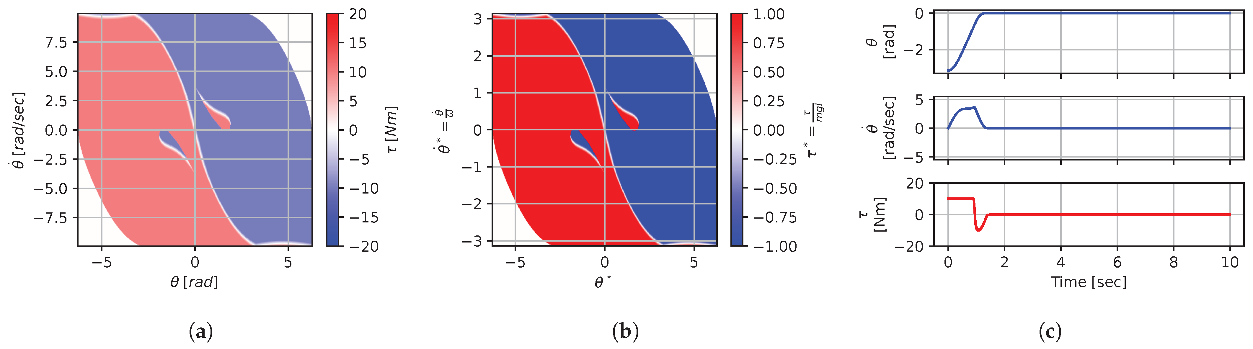
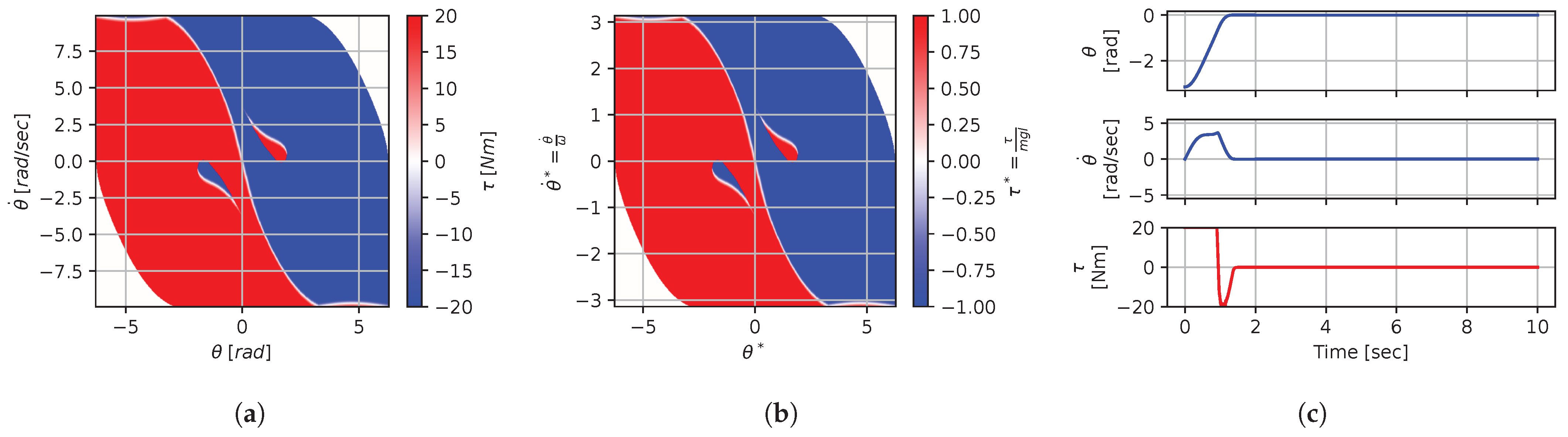
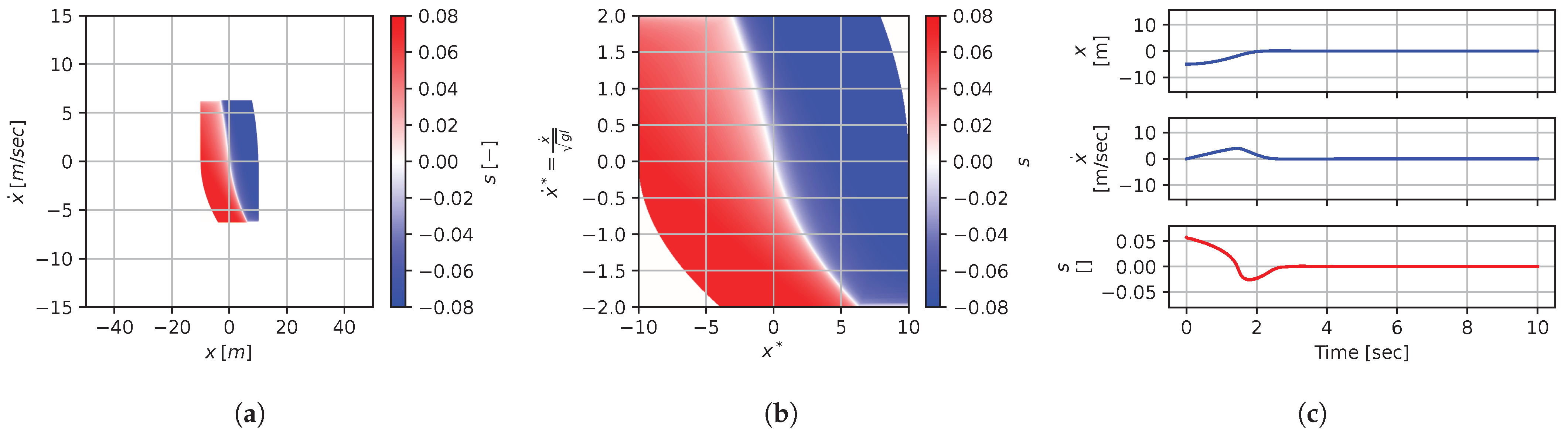
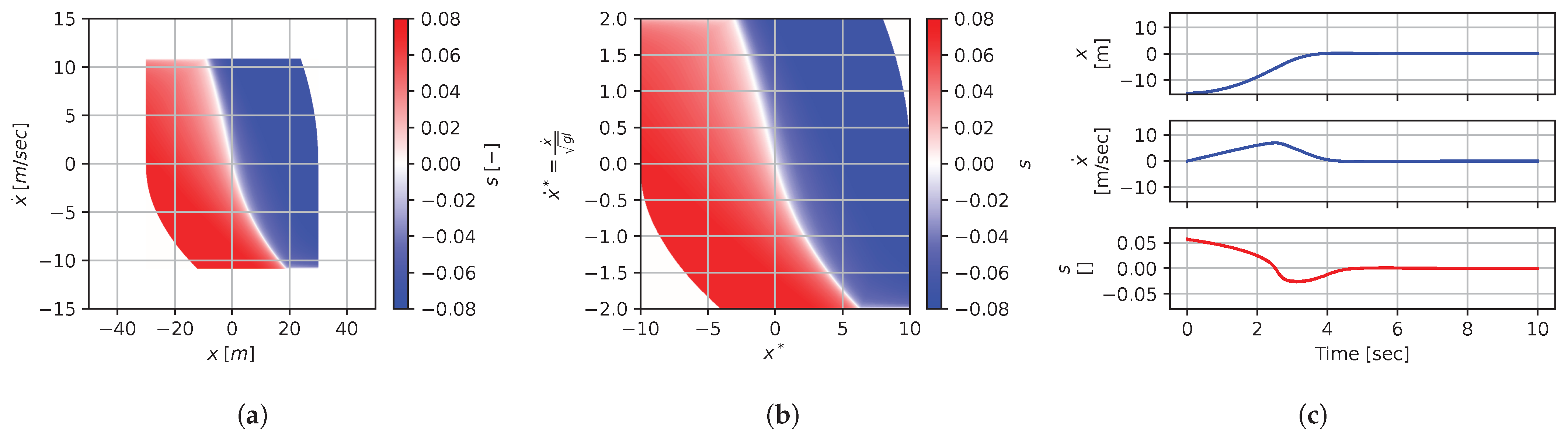
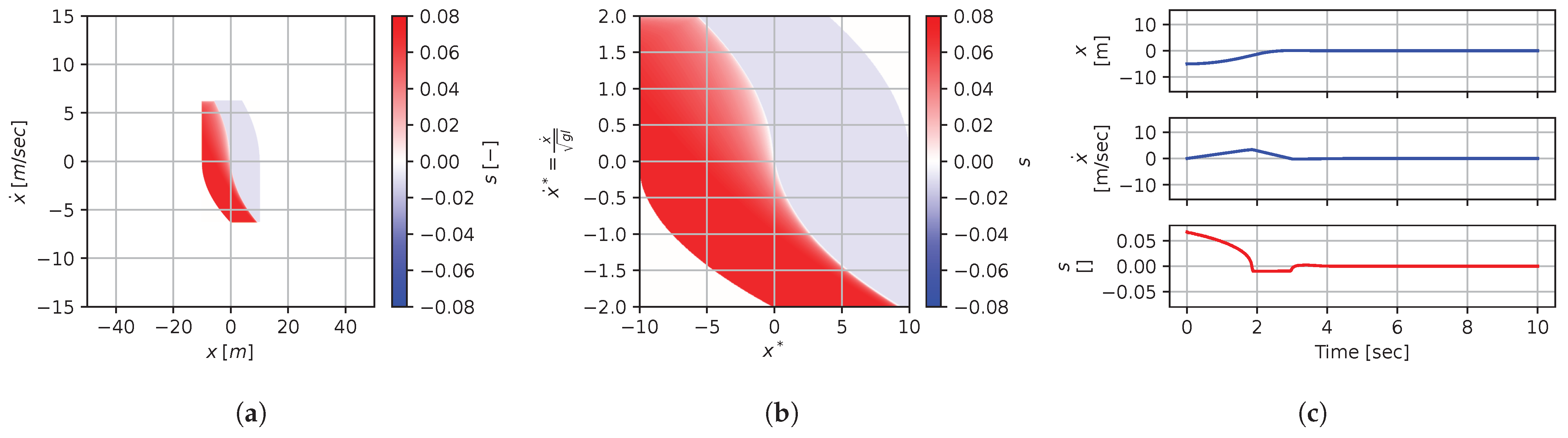
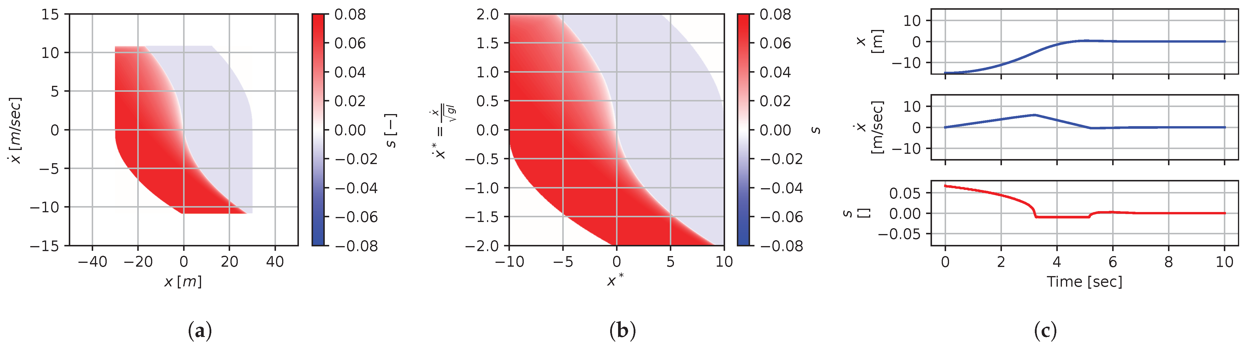
Figure 8.
Numerical results for context . (a) Feedback law f; (b) dimensionless feedback law ; (c) optimal trajectory, starting at .
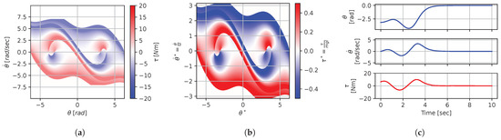
Figure 9.
Numerical results for context . (a) Feedback law f; (b) dimensionless feedback law ; (c) optimal trajectory, starting at .
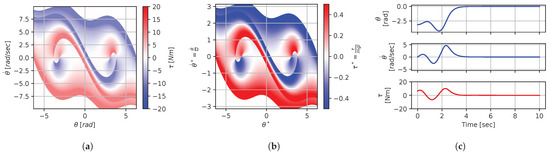
Figure 10.
Numerical results for context . (a) Feedback law f; (b) dimensionless feedback law ; (c) optimal trajectory, starting at .

Figure 11.
Numerical results for context . (a) Feedback law f; (b) dimensionless feedback law ; (c) optimal trajectory, starting at .

Figure 12.
Numerical results for context . (a) Feedback law f; (b) dimensionless feedback law ; (c) optimal trajectory, starting at .
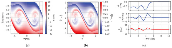
Figure 13.
Numerical results for context . (a) Feedback law f; (b) dimensionless feedback law ; (c) optimal trajectory, starting at .
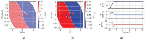
Figure 14.
Numerical results for context . (a) Feedback law f; (b) dimensionless feedback law ; (c) optimal trajectory, starting at .
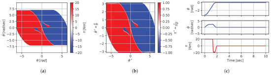
Figure 15.
Numerical results for context . (a) Feedback law f; (b) dimensionless feedback law ; (c) optimal trajectory, starting at .
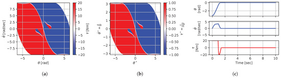
Figure 16.
Numerical results for context . (a) Feedback law f; (b) dimensionless feedback law ; (c) optimal trajectory, starting at .
In terms of how this can be applied in a practical scenario, we see that, if we compute the feedback law provided in Figure 8a, we can obtain the feedback law provided in Figure 9a directly by scaling the original policy with Equation (36) using the appropriate context variables, without having to recompute. In some sense, Equation (36) provides us with the ability to adjust the feedback law spontaneously to conform with new system parameters or , as would be the case with an analytical solution, even when working with black-box mapping, resulting in the form of a table look-up. However, the equivalence of the scaled solution is only guaranteed within a dimensionally similar context subset, which is the main limitation of this approach. The feedback law provided in Figure 8a cannot be scaled into the feedback law provided in Figure 14a, for instance, since and are not equals. It is also interesting to note that trajectory solutions from the same starting point—and computed cost-to-go functions (not illustrated)—are also all equivalent, up to scaling factors, within similar subgroups. Hence, optimal trajectories and cost-to-go solutions could also be shared and transferred between similar systems using the same technique that we demonstrate here for feedback laws.
3.1.4. Regimes of Solutions
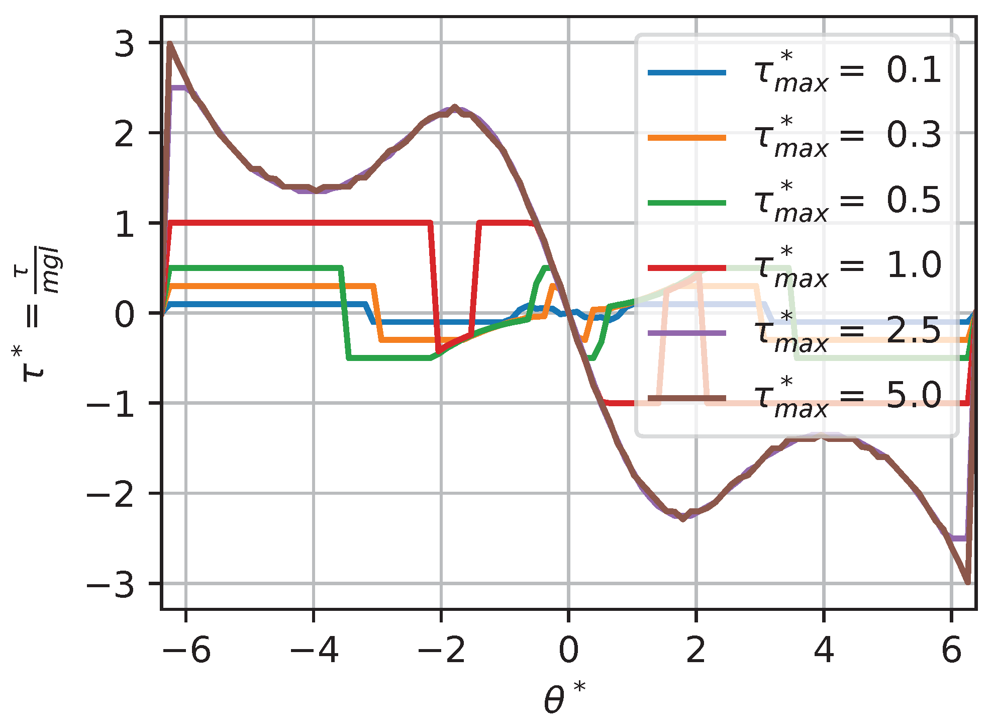
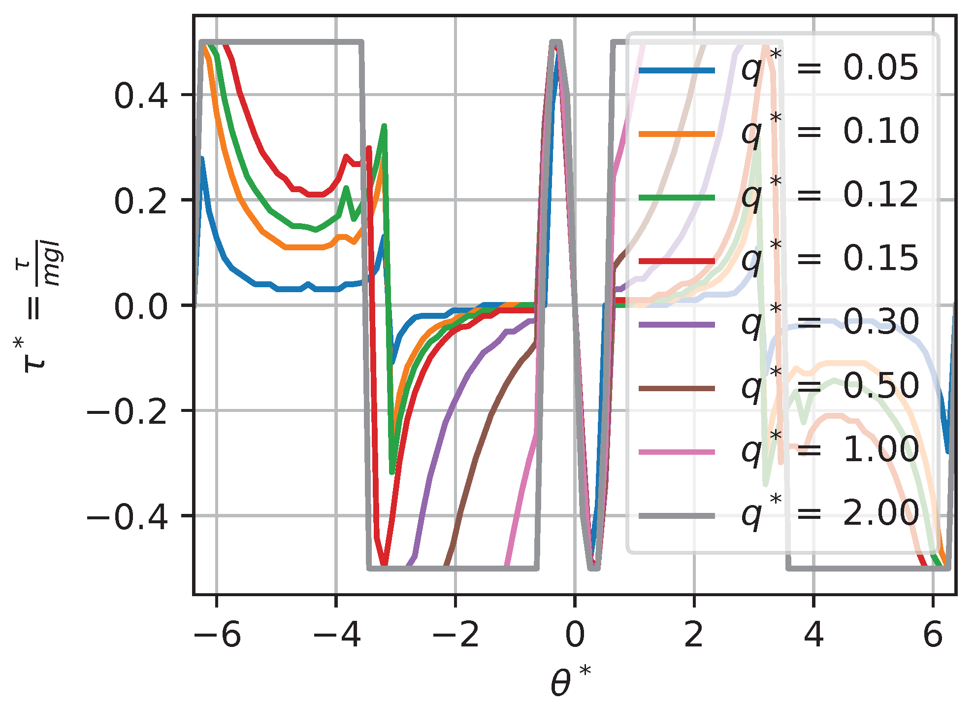
In some situations, changing a context variable will not have any effect on the optimal policy. For instance, for a torque-limited optimal pendulum swing-up problem, augmenting or q while keeping the other value fixed will have little effect above a given threshold. For instance, if we look at the solutions for contexts , , and , using a large amount of torque is so highly penalized by the cost function that the saturation limit does not have much impact on the solution (except for edge cases on the boundary). Thus, we would expect that augmenting would not change the solution. Figure 17 and Figure 18 show a slice (to allow for visualization) of the dimensionless optimal policy solution for various contexts. Figure 17 illustrates the results of changing while keeping fixed. We can see that, when , the policy is almost always on the min–max allowable torque values; this behavior is often called bang–bang. At the other extreme, when , the policy solution is continuous and almost never affected by the saturation. Figure 18 illustrates the results of changing while keeping fixed. We can see that, when , the optimal policy solution does not reach min–max saturation, while, when , the policy is almost always on the min–max allowable values.
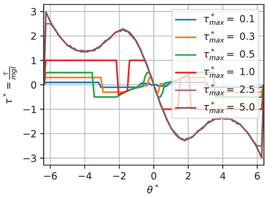
Figure 17.
Optimal dimensionless policy for various contexts: .

Figure 18.
Optimal dimensionless policy for various contexts: .
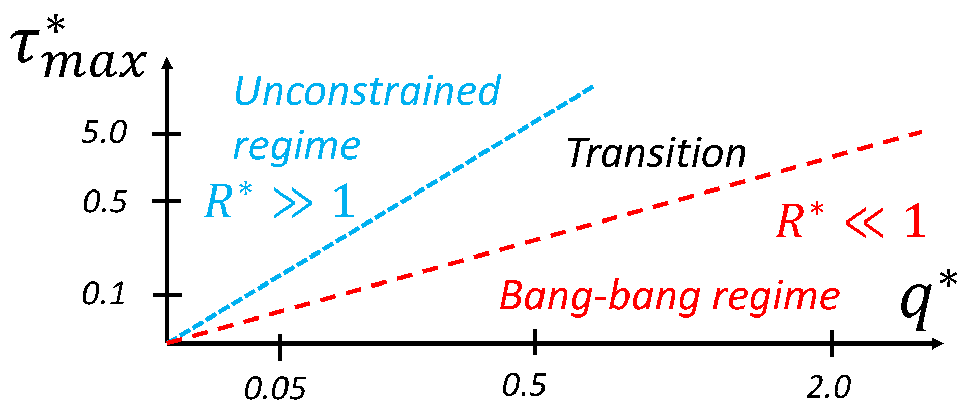
We can see that, for extreme context values, two types of behavior occur, illustrated as regions in the dimensionless context space in Figure 19. Those regions are best characterized by a ratio of and , a new dimensionless value that we define as the ratio of the maximum torque saturation over the weight parameter in the cost function q:
When the value of , the policy solution is partially continuous and reaches the min–max value in some other region of the state space; this is a behavior we call the transition regime. When the value of , the constraint on torque drives the solution to exhibit bang–bang behavior. In this region (that we approximate here, based on our sensitivity analysis, as ), the global policy is only a function of :
i.e., the value of does not affect the solution. On the other hand, when the value of , the policy is unconstrained. In this region (that we approximate here, based on our sensitivity analysis, as ), the global policy is only a function of since the constraint is so far away:
The concept of regime is often leveraged in fluid mechanics. It allows us to generalize results between situations where the relevant dimensionless numbers do not match exactly. For instance, when the Mach number is small (), we can generally assume an incompressible regime where various speeds of sound would not change the behavior much. Here, for the purpose of transferring policy solutions between contexts, this means that the condition of having the same exact dimensionless context variables can be relaxed with an inequality that corresponds to a regime. For instance, if we have two contexts in the unconstrained regime, it is sufficient to match only to create equivalent dimensionless policies.
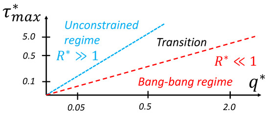
Figure 19.
Regime zones for a torque-limited pendulum swing-up problem.
Proposition 1.
If it is assumed that Equation (56) holds, the condition of having equivalent dimensionless feedback laws is relaxed to an inequality for one of the context variables as follows:
Proof.
First, if and , then from Equation (56) we can approximate the policy not to be a function of :
Hence, if , we have the following:
□
Also, for two contexts in a bang–bang regime, it is sufficient to match only to have equivalent dimensionless policies.
Proposition 2.
If it is assumed that Equation (55) holds, the condition of having equivalent dimensionless feedback laws is relaxed to an inequality for one of the context variables as follows:
Proof.
First, if and , then, from Equation (55), we can approximate the policy not to be a function of :
Hence, if , we have the following:
□
From another point of view, assuming one of those regimes means that we could have removed one variable from the context at the start of the dimensional analysis. All in all, the impact of identifying such regimes is that we can increase the size of the context subset to which the dimensionless version of the policy should be equivalent, leading to a potentially larger pool of systems that can share a learned policy and numerical results.
3.1.5. Methodology
We obtained the optimal feedback law presented in this section using a basic dynamic programming algorithm [18] on a discretized version of the continuous system. The approach is almost equivalent to the value iteration algorithm [5], which is sometimes referred to as model-based reinforcement learning, with the exception that, here, the total number of iteration steps was fixed (corresponding to a very long time horizon approximating an infinite horizon) instead of the iteration being stopped after reaching a convergence criterion. This approach was chosen to enable the collection of consistent results across all contexts, leading to a wide range of order-of-magnitude cost-to-go solutions. The time step was set to 0.025 s, the state space was discretized into an even 501 × 501 grid, and the continuous torque input was discretized into 101 discrete control options. Special out-of-bounds and on-target termination states were included to guarantee convergence [18]. Also, using dynamic programming made the setting of additional parameters to define the domain necessary. Although those parameters should not affect the optimal policy far away from the boundaries, dimensionless versions of those parameters were kept fixed in all the experiments as follows:
where is the range of angles for which the optimal policy is solved, set to one full revolution; is the range of angular velocity for which the optimal policy is solved; and is the time horizon, set to 20 periods of the pendulum using the natural frequency. The source code is available online at the following link: https://github.com/alx87grd/DimensionlessPolicies (accessed on 25 February 2024), and this Google Colab page allows users to reproduce the results: https://colab.research.google.com/drive/1kf3apyHlf5t7XzJ3uVM8mgDsneVK_63r?usp=sharing (accessed on 25 February 2024).
3.2. Optimal Motion for a Longitudinal Car on a Slippery Surface
The second numerical example is a simplified car positioning task. We use this example to illustrate that an optimal feedback law in the form of a table look-up generated for a car of a given size can be transferred to a car of a different size if the motion control problem is dimensionally similar, as illustrated at Figure 20. The example includes state constraints and a different type of non-linearity (i.e., not similar to the pendulum swing-up) to illustrate how generic the developed dimensionless polices concepts are.
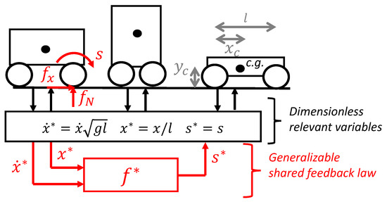
Figure 20.
Car positioning motion control problem.
3.2.1. Motion Control Problem
The motion control problem is defined here as finding a feedback law to control the dynamic system, as described by the following differential equation:
where is the ratio of vertical to horizontal forces on the front wheel, that is, a non-linear function of the front wheel slip s. The above equations represent a simple dynamic model of the longitudinal motion of a car, assuming that the controller can impose the wheel slip of the front wheel and that suspensions are infinitely rigid (but that weight transfer is included). Interestingly, it is already standard practice to model the ground–tire interaction with an empirical curve relating two dimensionless variables.
The objective is to minimize the infinite horizon quadratic cost function provided by the following:
subject to the constraints of keeping ground reaction forces positive, as provided by the following:
where the weight transfer potentially limits the allowable motions. Note that the cost function parameter q in this problem has a power of minus two to have a value with units of length, and all parameters are time-independent constants. The solution to this problem, i.e., the optimal policy for all contexts, involves the variables listed in Table 4 and should be of the form provided by
Table 4.
Longitudinal car optimal policy variables.
3.2.2. Dimensional Analysis
Here, we have one control input, two states, and five context parameters, for a total of variables. Of those variables, only independent dimensions (length and time ) are present. Using and as the repeated variables leads to the following dimensionless groups:
All three length variables are scaled by the wheel base, and the velocity variable is scaled using a combination of the wheel base and gravity. The transformation matrices are then as follows:
By applying the Buckingham theorem [4], Equation (74) can be restated as a relationship between the six dimensionless groups as follows:
3.2.3. Numerical Results
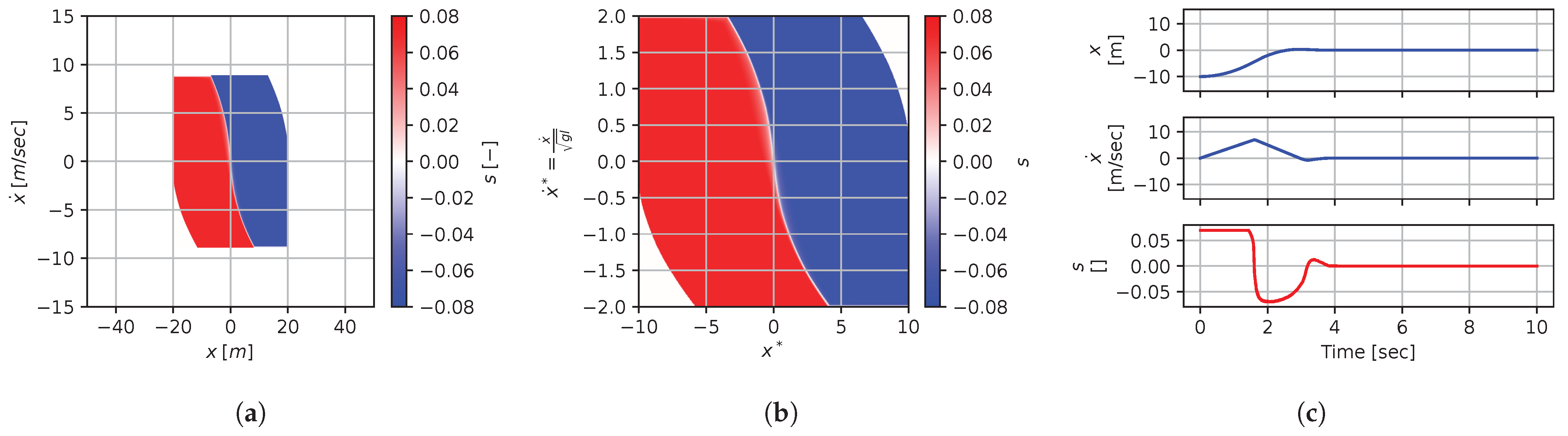
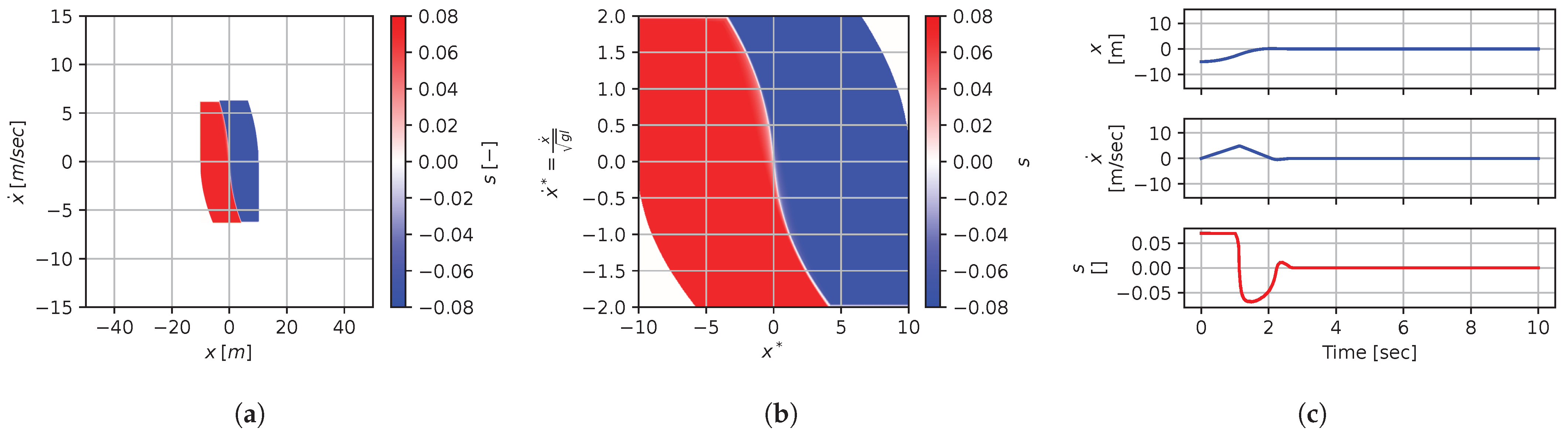
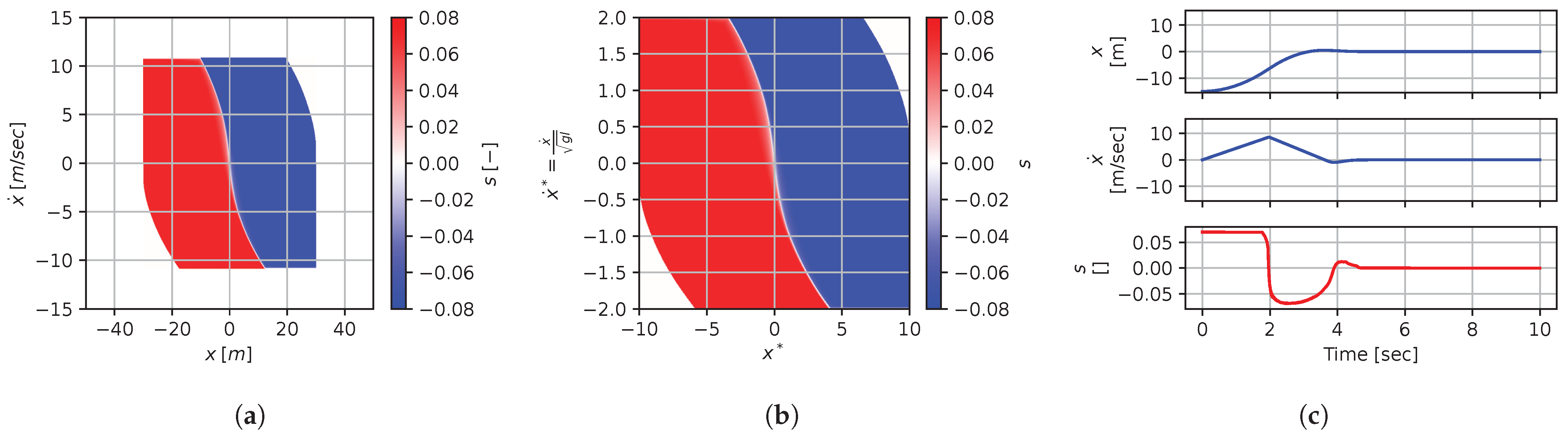
Here, as in the pendulum example, numerical solutions to the motion control problem are computed for the nine instances of context variables listed in Table 5. In those nine contexts, there are three subsets of three dimensionally similar contexts. Contexts , , and describe situations where the CG horizontal position is at half the wheel base; contexts , , and describe situations in which the the CG is very high (and hence the cars are very limited by the weight transfer); and contexts , , and describe situations in which position errors are highly penalized by the cost function plus cars with a very low CG relative to the wheel base.
Table 5.
Car problem parameters.
Figure 21, Figure 22, Figure 23, Figure 24, Figure 25, Figure 26, Figure 27, Figure 28 and Figure 29 illustrate that, for each subset with an equal dimensionless context, solutions are equal within each dimensionally similar subset when scaled into the dimensionless form. This was, again, the expected result predicted by the dimensional analysis presented in Section 2. In terms of how to use this in a practical scenario, this exemplifies how various cars (which are different but share the same ratios) could share a braking policy, for instance.

Figure 21.
Numerical results for context . (a) Feedback law f; (b) dimensionless feedback law ; (c) optimal trajectory, starting at .
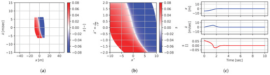
Figure 22.
Numerical results for context . (a) Feedback law f; (b) dimensionless feedback law ; (c) optimal trajectory, starting at .
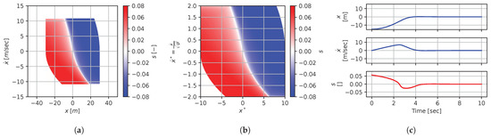
Figure 23.
Numerical results for context . (a) Feedback law f; (b) dimensionless feedback law ; (c) optimal trajectory, starting at .
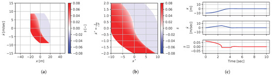
Figure 24.
Numerical results for context . (a) Feedback law f; (b) dimensionless feedback law ; (c) optimal trajectory, starting at .
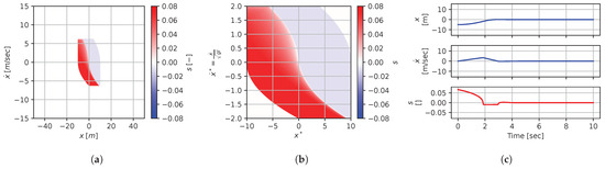
Figure 25.
Numerical results for context . (a) Feedback law f; (b) dimensionless feedback law ; (c) optimal trajectory, starting at .

Figure 26.
Numerical results for context . (a) Feedback law f; (b) dimensionless feedback law ; (c) optimal trajectory, starting at .
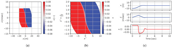
Figure 27.
Numerical results for context . (a) Feedback law f; (b) dimensionless feedback law ; (c) optimal trajectory, starting at .
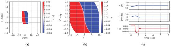
Figure 28.
Numerical results for context . (a) Feedback law f; (b) dimensionless feedback law ; (c) optimal trajectory, starting at .
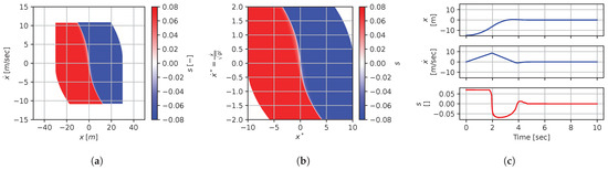
Figure 29.
Numerical results for context . (a) Feedback law f; (b) dimensionless feedback law ; (c) optimal trajectory, starting at .
3.2.4. Methodology
The same methodology as the pendulum example (see Section 3.1.5) was used for the car motion control problem. The time step was set to 0.025 s, the state space was discretized into an even 501 × 501 grid, and the continuous slip input was discretized into 101 discrete control options. Additional domain parameters were set as follows:
The source code is available online at the following link: https://github.com/alx87grd/DimensionlessPolicies (accessed on 25 February 2024), and this Google Colab page allows users to reproduce the results: https://colab.research.google.com/drive/1-CSiLKiNLqq9JC3EFLqjR1fRdICI7e7M?usp=share_link (accessed on 25 February 2024).
4. Case Studies with Closed-Form Parametric Policies
To better understand the concept of a dimensionless policy, in this section, two examples based on well-known closed-form solutions to classical motion control problems are presented to illustrate how using Theorem 2 can be equivalent to substituting new system parameters in an analytical solution.
4.1. Dimensionless Linear Quadratic Regulator
The first example is based on the linear quadratic regulator (LQR) solution [19] for the linearized pendulum that allows for a closed-form analytical solution of optimal policy. This allows us to compare the method of transferring the policy with the proposed scaling law of Equation (36) to the method of transferring the policy by substituting the new system parameters in the analytical solution.
Here, we consider a simplified version of the pendulum swing-up problem (see Section 3.1), and a linearized version of the equation of motion is used as follows:
The same infinite horizon quadratic cost function is used, as follows:
However, no constraints on the torque are included in this problem. All parameters are also assumed to be time-independent constants. The same variables are used in this problem definition as before, except that the torque limit variable is absent. The global policy solution should then have the following form:
We can thus select the same dimensionless groups as in Section 3.1.2 and conclude that Equation (90) can be restated under the following dimensionless form:
Proposition 3.
Proof.
See Appendix A. □
Applying Equation (31) to this feedback law leads to the dimensionless form, using and for shortness, as follows:
The dimensionless policy is only a function of the dimensionless states and the dimensionless cost parameter , as predicted by Equation (91) based on the dimensional analysis. It is interesting to note that Equation (96) represents the core generic solution to the LQR problem and is independent of unit and scale.
We can also use this analytical policy solution to demonstrate Theorem 2, i.e., show that scaling the policy with Equation (36) is equivalent to substituting new context variables when the contexts are dimensionally similar.
Proposition 4.
Proof.
This example illustrates that applying the scaling of Equation (36) based on the dimensional analysis framework is equivalent to changing the context variables in an analytical solution when the dimensionless context variables are equal.
4.2. Dimensionless Computed Torque
The second example is again based on the pendulum but using the computed torque control technique [20]. This also allows us to compare the method of transferring the policy with the proposed scaling law of Equation (36) to the method of transferring the policy by substituting the new system parameters in the analytical solution. This example is not based on a quadratic cost function, as opposed to previous examples, to illustrate the flexibility of the proposed schemes.
Here, we present a second analytical example. A computed torque feedback law is a model-based policy (assuming that there are no torque limits) that is the solution to the motion control problem of making a mechanical system that converges on a desired trajectory, with a specified second-order exponential time profile defined by the following equation:
For the specific case of the pendulum swing-up problem, we assume that all parameters are time-independent constants and that our desired trajectory is simply the upright position (), leaving only two parameters to define the tasks: and . Then, the computed torque policy takes the following form:
and the analytical solution is as follows:
Here, the context includes the system parameters and two variables characterizing the convergence speed. Note that the task parameters directly define the desired behavior, as opposed to the previous examples where they were defining the behavior indirectly through a cost function. The states, control inputs, and system parameters are the same as before; only the task parameters differ, and their dimensions are presented in Table 6.
Table 6.
Computed torque task variables.
Here, seven variables and only independent dimensions ( and ) are involved. Thus, five dimensionless groups can be formed, as follows:
Using and , the system parameters, as the repeating variables leads to the following dimensionless groups:
Then, applying the Buckingham theorem tells us that the computed torque policy can be restated as the following relationship between the dimensionless variables:
Here, we can confirm directly (since we have an analytical solution) that applying Equation (31) to the computed torque feedback law provided by Equation (109) leads to the following dimensionless form:
thereby confirming the structure predicted by Equation (116) based on the dimensional analysis.
We can, again, use this example to demonstrate Theorem 2 and show that, when the dimensionless context is equal, scaling a policy using Equation (36) is equivalent to substituting new values of the system parameters into the analytical equation.
Proposition 5.
Proof.
If we substitute in Equation (121) by the analytical solution provided by Equation (119) and then distribute the multiplying scaling factors, we obtain
which is exactly equivalent to Equation (120) (i.e., equivalent to substituting the a instance of the context variables to the b instance) if
which is the dimensional similarity condition () for this motion control problem:
□
5. Conclusions
The dimensional analysis of physically meaningful control policies, leveraging the Buckingham theorem, leads to two interesting theoretical results. (1) In dimensionless form, the solution to a motion control problem involves a reduced number of parameters. (2) It is possible to exactly transfer a feedback law between similar systems without any approximation, simply by scaling the input and output of any type of control law appropriately, including via numerically generated black-box mapping. However, the main practical limitation of this approach is that, if the condition of dimensional similarity () is not met exactly, then there are no theoretical guarantees regarding whether a policy is transferable without additional assumptions, such as with the discussed concept of regimes of behavior. Also, we demonstrated how those results can be used to exactly transfer even discontinuous black-box policies between similar systems using two simple examples of dynamical systems and numerically generated optimal feedback laws. An interesting direction for further exploration would be investigating how good an approximation is when a feedback law is transferred from a context that is not exactly the same but close. Also, it would be interesting to test the concept of dimensionless policies to empower a reinforcement learning scheme that could collect data from various, but dimensionally similar, systems to accelerate the learning process.
Funding
This research was funded by NSERC discovery grant number RGPIN-2018-05388.
Data Availability Statement
The source code used to generate numerical results in this paper is available link: https://github.com/alx87grd/DimensionlessPolicies (accessed on 25 February 2024).
Conflicts of Interest
The authors declare no conflicts of interest.
Abbreviations
The following abbreviations are used in this manuscript:
| CG | Center of gravity |
| CT | Computed torque |
| LQR | Linear quadratic regulator |
Appendix A. LQR Analytic Solution
In this section, we show that the policy provided by Equation (92) is optimal with respect to the LQR problem defined in Section 4.1. We can write the equation of motion provided by Equation (88) in state-space form, using and , as follows:
Then, by adapting a solution from [21], if we parameterize the weight matrix of the cost function as follows:
the optimal cost-to-go is provided by the following:
and the optimal feedback policy is provided by
This solution can by verified by substituting matrices into the algebraic Riccati equation provided by
since the problem fits into the framework of the classical infinite horizon LQR result [18]. Then, we can see that the cost function defined in Section 4.1 is a special case, where and , leading to the following equations:
Solving for a and b, and retaining the positive solution, leads to the following:
which, when substituted into Equation (A4), is equal to the policy provided by Equation (92) in Section 4.1.
References
- Kuindersma, S.; Deits, R.; Fallon, M.; Valenzuela, A.; Dai, H.; Permenter, F.; Koolen, T.; Marion, P.; Tedrake, R. Optimization-based locomotion planning, estimation, and control design for the atlas humanoid robot. Auton. Robot. 2016, 40, 429–455. [Google Scholar] [CrossRef]
- Schwenzer, M.; Ay, M.; Bergs, T.; Abel, D. Review on model predictive control: An engineering perspective. Int. J. Adv. Manuf. Technol. 2021, 117, 1327–1349. [Google Scholar] [CrossRef]
- Rudin, N.; Hoeller, D.; Reist, P.; Hutter, M. Learning to Walk in Minutes Using Massively Parallel Deep Reinforcement Learning. In Proceedings of the 5th Conference on Robot Learning, London, UK, 8–11 November 2021; pp. 91–100. [Google Scholar]
- Buckingham, M.E. On Physically Similar Systems; Illustrations of the Use of Dimensional Equations. Phys. Rev. 1914, 4, 345. [Google Scholar] [CrossRef]
- Sutton, R.S.; Barto, A.G. Reinforcement Learning: An Introduction, 2nd ed.; Bradford Books: Cambridge, MA, USA, 2018. [Google Scholar]
- Taylor, M.E.; Stone, P. Transfer Learning for Reinforcement Learning Domains: A Survey. J. Mach. Learn. Res. 2009, 10, 1633–1685. [Google Scholar]
- Devin, C.; Gupta, A.; Darrell, T.; Abbeel, P.; Levine, S. Learning modular neural network policies for multi-task and multi-robot transfer. In Proceedings of the 2017 IEEE International Conference on Robotics and Automation (ICRA), Singapore, 29 May–3 June 2017; pp. 2169–2176. [Google Scholar] [CrossRef]
- Gupta, A.; Devin, C.; Liu, Y.; Abbeel, P.; Levine, S. Learning Invariant Feature Spaces to Transfer Skills with Reinforcement Learning. arXiv 2017, arXiv:1703.02949. [Google Scholar]
- Helwa, M.K.; Schoellig, A.P. Multi-robot transfer learning: A dynamical system perspective. In Proceedings of the 2017 IEEE/RSJ International Conference on Intelligent Robots and Systems (IROS), Vancouver, BC, Canada, 24–28 September 2017; pp. 4702–4708. [Google Scholar] [CrossRef]
- Chen, T.; Murali, A.; Gupta, A. Hardware Conditioned Policies for Multi-Robot Transfer Learning. In Proceedings of the 32nd Conference on Neural Information Processing Systems (NeurIPS 2018), Montréal, QC, Canada, 2–8 December 2018; Curran Associates, Inc.: Red Hook, NY, USA, 2018; Volume 31. [Google Scholar]
- Pereida, K.; Helwa, M.K.; Schoellig, A.P. Data-Efficient Multirobot, Multitask Transfer Learning for Trajectory Tracking. IEEE Robot. Autom. Lett. 2018, 3, 1260–1267. [Google Scholar] [CrossRef]
- Sorocky, M.J.; Zhou, S.; Schoellig, A.P. Experience Selection Using Dynamics Similarity for Efficient Multi-Source Transfer Learning Between Robots. arXiv 2020, arXiv:2003.13150. [Google Scholar] [CrossRef]
- Bertrand, J. Sur l’homogénéité dans les formules de physique. Cah. Rech. L’Acad. Sci. 1878, 86, 916–920. [Google Scholar]
- Rayleigh, L. VIII. On the question of the stability of the flow of fluids. Lond. Edinb. Dublin Philos. Mag. J. Sci. 1892, 34, 59–70. [Google Scholar] [CrossRef]
- Bakarji, J.; Callaham, J.; Brunton, S.L.; Kutz, J.N. Dimensionally consistent learning with Buckingham Pi. Nat. Comput. Sci. 2022, 2, 834–844. [Google Scholar] [CrossRef] [PubMed]
- Fukami, K.; Taira, K. Robust machine learning of turbulence through generalized Buckingham Pi-inspired pre-processing of training data. In Proceedings of the APS Division of Fluid Dynamics, Phoenix, AZ, USA, 21–23 November 2021; Meeting Abstracts ADS Bibcode: 2021APS..DFDA31004F. p. A31.004. [Google Scholar]
- Xie, X.; Samaei, A.; Guo, J.; Liu, W.K.; Gan, Z. Data-driven discovery of dimensionless numbers and governing laws from scarce measurements. Nat. Commun. 2022, 13, 7562. [Google Scholar] [CrossRef] [PubMed]
- Bertsekas, D.P. Dynamic Programming and Optimal Control: Approximate Dynamic Programming; Athena Scientific: Nashua, NH, USA, 2012. [Google Scholar]
- Kalman, R.E. Contributions to the theory of optimal control. Bol. Soc. Mat. Mex. 1960, 5, 102–119. [Google Scholar]
- Asada, H.H.; Slotine, J.J.E. Robot Analysis and Control; John Wiley & Sons: New York, NY, USA, 1986. [Google Scholar]
- Hanks, B.; Skelton, R. Closed-form solutions for linear regulator-design of mechanical systems including optimal weighting matrix selection. In Proceedings of the 32nd Structures, Structural Dynamics, and Materials Conference, Baltimore, MD, USA, 8–10 April 1991. [Google Scholar] [CrossRef]


Disclaimer/Publisher’s Note: The statements, opinions and data contained in all publications are solely those of the individual author(s) and contributor(s) and not of MDPI and/or the editor(s). MDPI and/or the editor(s) disclaim responsibility for any injury to people or property resulting from any ideas, methods, instructions or products referred to in the content. |
© 2024 by the author. Licensee MDPI, Basel, Switzerland. This article is an open access article distributed under the terms and conditions of the Creative Commons Attribution (CC BY) license (https://creativecommons.org/licenses/by/4.0/).