Tensor-Based Sparse Representation for Hyperspectral Image Reconstruction Using RGB Inputs

Abstract

Hyperspectral image (HSI) reconstruction from RGB input has drawn much attention recently and plays a crucial role in further vision tasks. However, current sparse coding algorithms often take each single pixel as the basic processing unit during the reconstruction process, which ignores the strong similarity and relation between adjacent pixels within an image or scene, leading to an inadequate learning of spectral and spatial features in the target hyperspectral domain. In this paper, a novel tensor-based sparse coding method is proposed to integrate both spectral and spatial information represented in tensor forms, which is capable of taking all the neighboring pixels into account during the spectral super-resolution (SSR) process without breaking the semantic structures, thus improving the accuracy of the final results. Specifically, the proposed method recovers the unknown HSI signals using sparse coding on the learned dictionary pairs. Firstly, the spatial information of pixels is used to constrain the sparse reconstruction process, which effectively improves the spectral reconstruction accuracy of pixels. In addition, the traditional two-dimensional dictionary learning is further extended to the tensor domain, by which the structure of inputs can be processed in a more flexible way, thus enhancing the spatial contextual relations. To this end, a rudimentary HSI estimation acquired in the sparse reconstruction stage is further enhanced by introducing the regression method, aiming to eliminate the spectral distortion to some extent. Abundant experiments are conducted on two public datasets, indicating the considerable availability of the proposed framework.

1. Introduction

With the continuous development of remote sensing technology, a variety of new optical sensors have been applied to promote the development of hyperspectral imaging technology [1]. Compared with the traditional visible image, hyperspectral images (HSIs) are characterized by a higher spectral resolution, which can reach the nanometer level. HSIs can not only reflect the external features of an observed target, such as its shape and texture, but also contain spectral information that can further distinguish different substances. Therefore, HSIs have been successfully applied to various fields due to their high development potential and application value, including agriculture [2], pathological detection [3], the military [4], environmental governance [5] and so on. In addition, hyperspectral imaging technology further promotes the development of computer vision to a great extent, such as target detection [6], target tracking [7,8], target classification [9,10] and other high-level tasks [11,12,13,14,15].

At present, HSIs are mainly obtained using imaging spectrometers [16]. Imaging spectrometers use traditional imaging techniques to capture relevant information of targets in the spatial space and capture the intrinsic spectral features of targets through specific spectral sensors synchronously. Notably, the spectral resolution is highly dependent on the performance of the imaging spectrometer, which can range from tens to hundreds of bands. However, the great cost and technology seriously limit the acquisition of HSIs with both high spectral and spatial resolutions synchronously, which further hinders the application of hyperspectral imaging to a great extent. Therefore, obtaining HSIs with a high quality at a low cost is crucial to the development of remote sensing.

Recently, with the great progress in computational imaging, various software algorithms have been proposed to tackle the issues in the acquisition of HSIs with a high quality, thus reducing the requirements for imaging spectrometers. According to the requirement of inputs, the hyperspectral computational imaging method can be roughly summarized as multi-source-based spectral super-resolution imaging [17,18,19,20] and single-source-based spectral super-resolution imaging [21,22,23,24,25,26,27,28,29,30,31,32,33,34,35,36]. The multi-source-based method mainly focuses on developing the fusion strategies of two paired images, of which one is at a high spatial resolution, while the other one is at a high spectral resolution. The multi-source-based method comprehensively combines the two complementary advantages and outputs the fused HSI, achieving a considerable performance. Nevertheless, these kinds of methods are limited in practical situations due to the uneasy acquisition of paired images. Therefore, the single-source-based method, which mainly reconstructs the target HSI from its corresponding RGB image, has drawn more and more attention. On one hand, the RGB images can be easily captured through consumer cameras. On the other hand, there is a certain pixel-wise relation between an RGB image and its corresponding HSI [37]. Previously, regression-based methods, such as the Radial basis function [22], made the first attempt to solve the three-to-many ill-posed problem through establishing a linear mapping function, by which the reconstructed results cannot meet the requirements of further applications. Nowadays, the single-source-based method can be roughly divided into the sparse coding-based algorithm and the deep learning-based framework. Although the deep learning-based method is capable of reconstructing the target HSI with a higher accuracy, its final performance is highly dependent on the training data. The sparse coding-based algorithm uses hyperspectral prior data to construct a feature sparse dictionary, which is then mapped to obtain the RGB projected sparse dictionary and its corresponding coefficients; thus, the target HSI can be reconstructed using the calculated coefficients. Compared with the learning-based method, the sparse coding method is able to generate considerable results using less data. In addition, the sparse coding method has a more reasonable interpretability.

Current sparse coding-based methods often conduct the reconstruction process in a pixel-wise manner, which could break the original structure of input RGB images, leading to an insufficient retainment of spatial and spectral information in the target hyperspectral space. In this paper, a tensor-based sparse representation for hyperspectral image reconstruction is proposed that integrates the complemental spectral and spatial features enclosed in the RGB inputs as depicted in Figure 1. Specifically, the proposed method achieves the whole process in a tensor-wise way, which treats each group of neighboring pixels as a whole instead of splitting the original RGB inputs into several pixels, aiming to avoid breaking the local data structure to some extent. In this way, the traditional spectral vector is represented as a three-dimensional tensor, through which more information can be comprehensively considered during the whole process. To this end, the proposed method mainly contains three stages: tensor dictionary learning, sparse reconstruction and spectral enhancement. In the tensor dictionary learning stage, prior tensor training pixels are used to train a high-dimensional HSI tensor dictionary, and the well-trained dictionary is then projected to the RGB domain. In the sparse reconstruction stage, a rudimentary HSI estimation can be acquired by solving the sparse problem. Finally, a regression method is introduced to enhance the HSI spectral features, thus avoiding the spectral distortion to some extent. In summary, the primary contributions are as follows:

Figure 1. Hyperspectral image pixel tensorization.

(1)

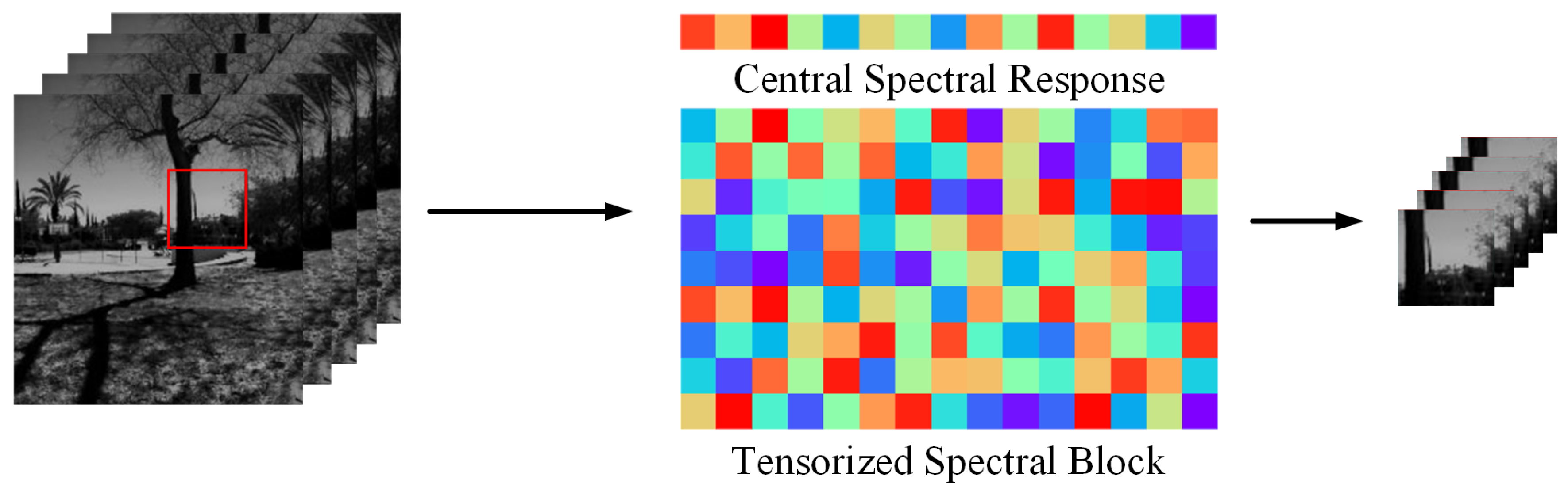
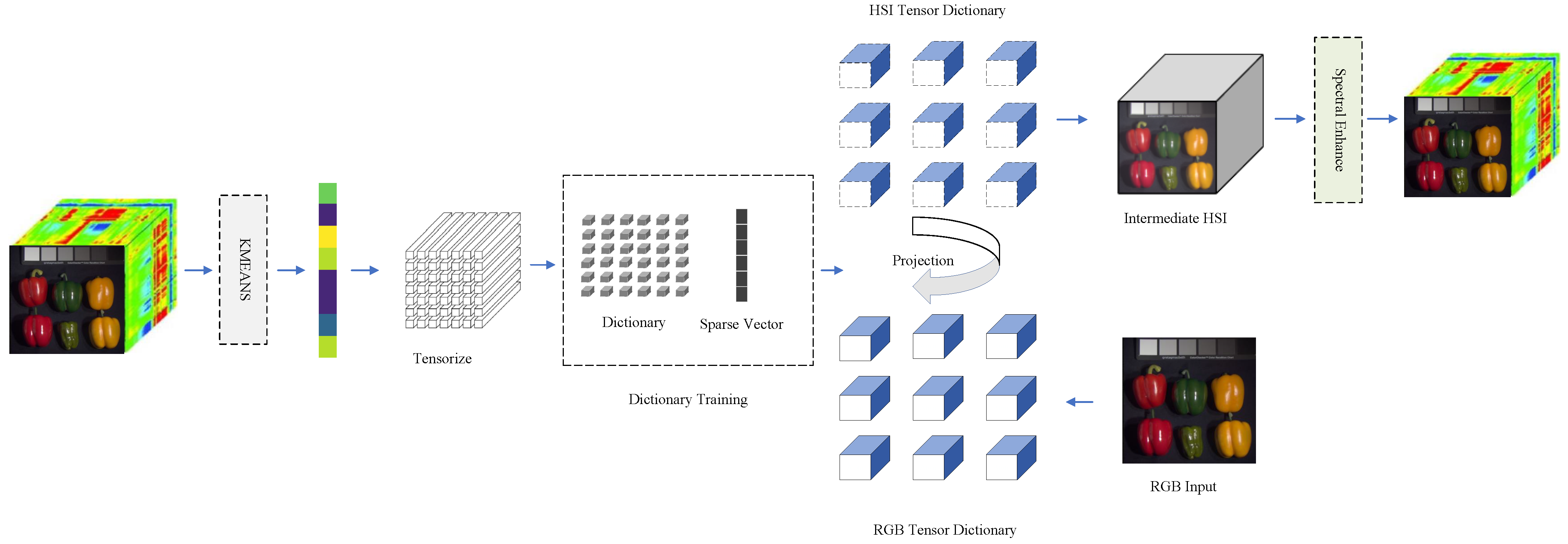
A novel tensor-based sparse representation framework is proposed for reconstructing HSIs from the corresponding RGB images through making full use of the tensor-wise representations to describe the spectral data, by which the structure of original inputs can be retained in a more flexible way, thus enhancing the spatial contextual relations.

(2)

A preprocessing method based on the clustering strategy is devised to reduce the redundancy of spectral training datasets, enhancing the representativeness of the target spectral dictionary.

(3)

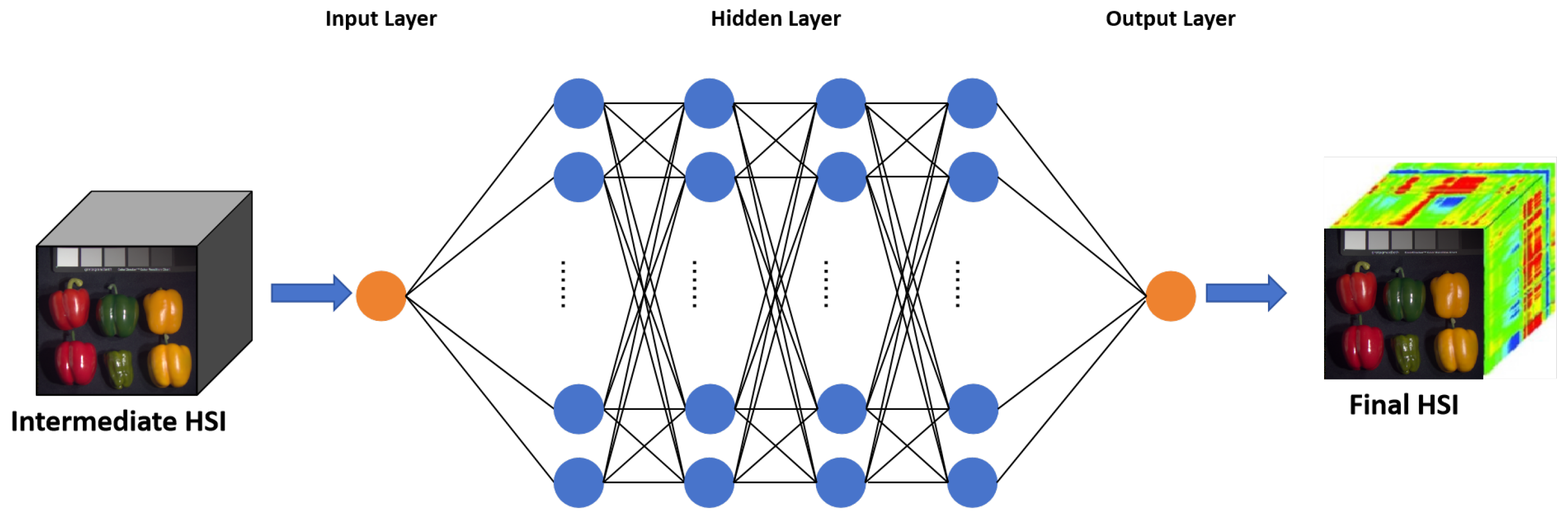
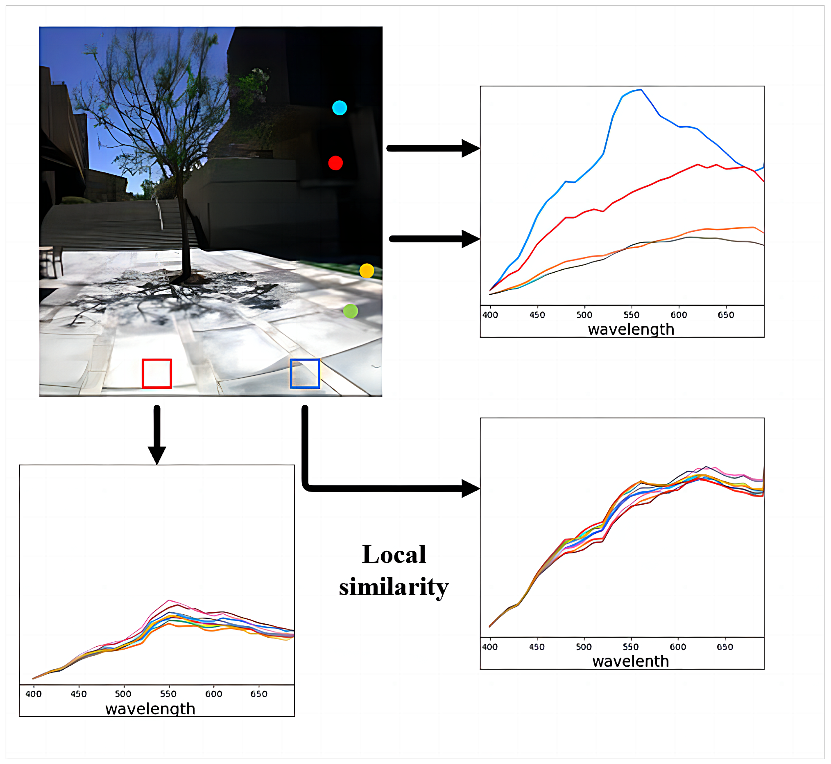
A spectral enhancement strategy is deployed to further mitigate the spectral distortion in the junction of two different image regions through introducing the regression method.

(4)

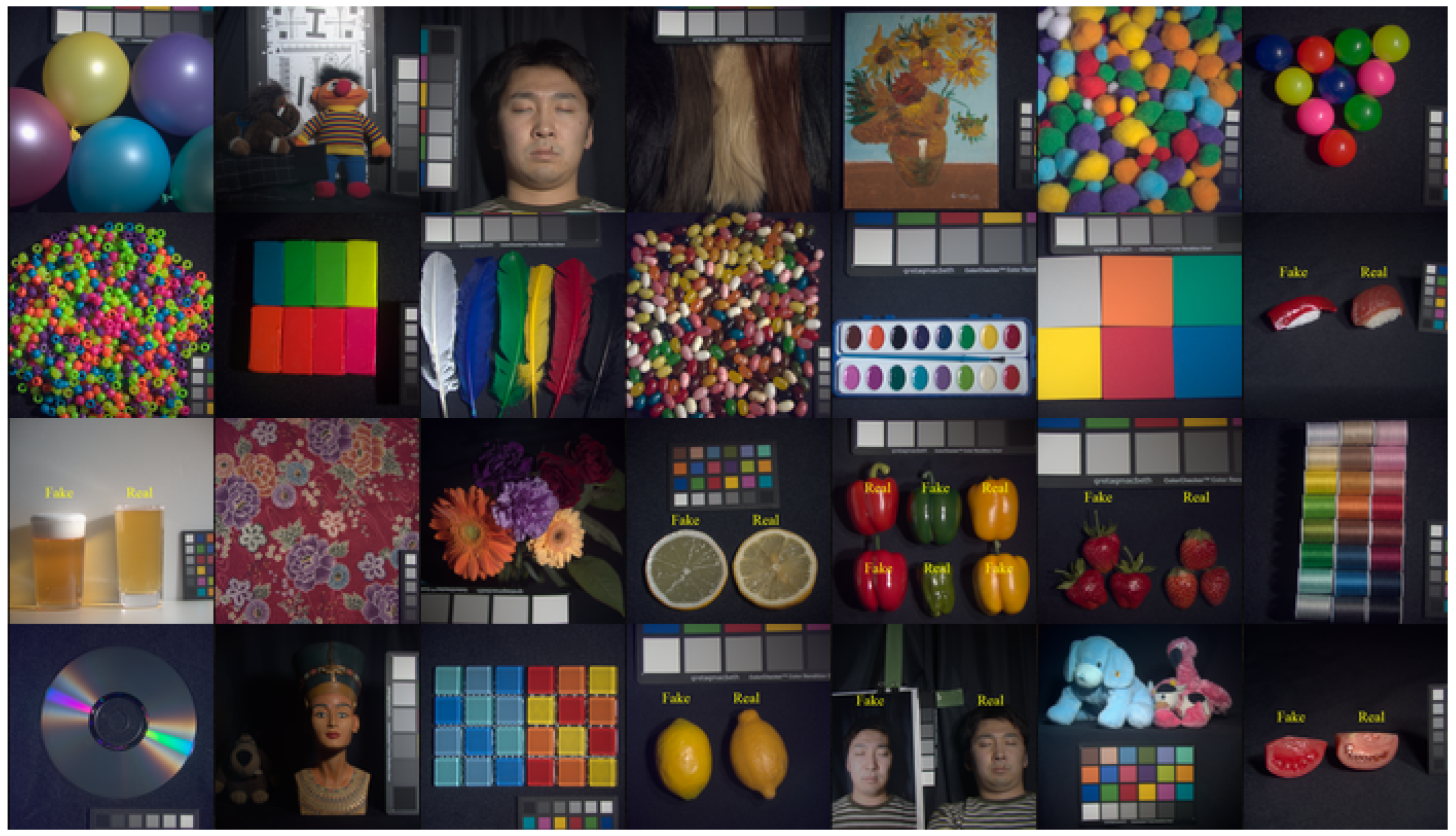
Extensive quantitative and qualitative experiments are conducted over two benchmark datasets under multiple evaluation metrics, demonstrating the availability of our proposed method.

The rest of this paper is organized as follows. Section 2 gives a brief illustration of related works. Section 3 presents the preliminaries of the image reconstruction field and tensor algebra. In Section 4, a description of the proposed approach is given in detail. Quantitative and qualitative experimental results are both demonstrated in Section 5. The conclusion is drawn in Section 6.

2. Related Work

2.1. CNN-Based Reconstruction Methods

Since the convolutional neural network (CNN) was proposed, it has been exploited in many tasks, including image classification [38,39], object detection and so on [40]. Similarly, the CNN also plays a crucial role in the SSR process, which has drawn much attention recently. The CNN-Based Hyperspectral Image Recovery from Spectrally Undersampled Projections named HSCNN can be treated as the most representative CNN-based SSR method, which mainly consists of five convolutional layers and is capable of reconstructing the target HSI from its corresponding RGB inputs [29]. SR2D/3DNet was proposed in the NTIRE2018 challenge, which comprehensively takes into consideration spectral and spatial feature learning through combining the 2D and 3D structure [30]. In addition, the U-Net architecture has also been proved to be effective for the SSR and is capable of refining the spatial and spectral features in a coarse-to-fine manner [26,27,28]. In [28], Zhao et al. introduced the multi-scale strategy into the SSR, which adopted the PixelShuffle operation to form a novel four-level hierarchical regression network (HRNet) to extract features at different resolutions, thus obtaining the local and global learning capacities. Li et al. combined the attention mechanism into the SSR process, processing a deep hybrid 2D-3D CNN with dual second-order attention, which is able to focus on prominent spatial and spectral features [31]. Peng et al. proposed a pixel attention mechanism to explore the pixel-wise features through the global average pooling operation [32]. However, these CNN-based methods all require a large number of paired HSIs and RGB images as a training set to ensure the SSR performance, which lacks interpretability to some extent. In addition, the physical consistency of the network suffers from the various external factors enclosed in the RGB inputs, including the noises and lighting condition, which may lead to a lack of robustness in all CNN-based SSR methods.

2.2. Sparse Coding-Based Methods

The sparse coding-based methods exploit the prior distribution of hyperspectral signatures in natural images, where the spectral reflectance is mainly decided by the material and illumination [41]. Building an over-complete dictionary is the conventional way, which makes it possible to reconstruct the target HSIs. In 2016, Arad and Ben-Shahar firstly performed the SSR process through using a single RGB image as input, which trained an over-complete dictionary with prior spectral data [21]. On this basis, the well-trained dictionary is then projected onto the RGB space through the specific color response function, which is further solved to obtain the sparse coefficients, thus reconstructing the final HSIs. The final reconstruction performance by Arad’s method is highly dependent on the prior spectral dictionary, whose quality seriously affects the accuracy of the reconstructed HSIs. Chen Yi et al. restored the corresponding data by establishing sub-dictionaries of each band on the basis of Arad, obtaining HSIs with a higher accuracy [33]. However, this method takes a huge amount of computation, leading to a poor performance on instantaneity. Motivated by the A+ method [34], Aeschbacher et al. established strong shallow baselines for HSI reconstruction from RGB inputs, obtaining a considerable reconstruction result with a better accuracy and runtime [23].

In comparison with these methods, our proposed framework makes the first attempt to conduct the SSR process in a tensor-wise manner instead of splitting the scenes or targets with abundant semantic information into several meaningless pixels, and it is able to retain the data structure as much as possible, thus representing the spatial–spectral features in a more consistent way. It is worth noting that a conference version of this paper has been published in [42], and significant modifications are as follows: (1) a data preprocess strategy is proposed to enhance the representativeness of the spectral dictionary; (2) more descriptions of our proposed method are given in detail; (3) a spectral enhancement strategy is devised to further remit the spectral distortion; (4) more comprehensive experiments are conducted to verify the validity of the proposed framework.

3. Preliminaries

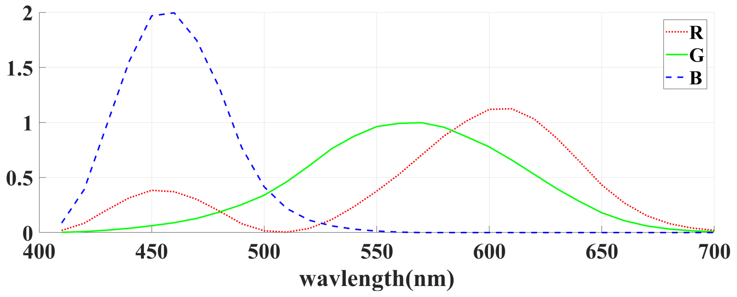
3.1. Problem Formulation

Two essential factors that determine the formation of an image are the scene light source and image capturing device (e.g., camera). The spectral energy emitted by the source of light is cast onto the object, where a portion of the energy is then reflected. Subsequently, the sensor in the camera receives the reflected energy to render the final image. In this process, the brightness of the image is measured by the intensity of the light source, while the sharpness and color reproduction are directly influenced by the responsiveness of the camera sensor. To model the imaging formation in a mathematical way, we can process the information of the light source, spectral reflectance and camera spectral sensitivity simultaneously by integrating the multiplication of them to calculate the camera response.

$$X_i={\int }_{\lambda }E\left(\lambda \right)R\left(\lambda \right)C\left(\lambda \right)d\lambda ,i=r,g,b,$$

(1)

where $E\left(\lambda \right)$ represents the spectral energy distribution of the scene light source, $R\left(\lambda \right)$ is the surface reflection coefficient and $C\left(\lambda \right)$ is the i-th channel of the color match function. For example, $\mathcal{X}\in {\mathbb{R}}^{I_1\times I_2\times \dots \times I_n}$ means an nth-order tensor, whose $(i_1,i_2,\dots ,i_n)$ element is ${\mathcal{X}}_{i_1{i}_2\dots i_n}$. In addition, the $E\left(\lambda \right)R\left(\lambda \right)$ stands for the object’s spectrum reflection, which can be easily acquired using an imaging spectrometer. Therefore, Equation (1) can be rewritten as follows:

$$\begin{array}{cc}\hfill & X_i={\int }_{\lambda }S\left(\lambda \right)C\left(\lambda \right)d\lambda ,i=r,g,b,\hfill \\ \hfill & S\left(\lambda \right)=E\left(\lambda \right)R\left(\lambda \right),\hfill \end{array}$$

(2)

More specifically, the RGB image can be denoted as $\mathit{X}\in {\mathbb{R}}^{r\times c\times 3}$ composed of $r\times c$ pixels, and the corresponding HSI is represented as $\mathit{Y}\in {\mathbb{R}}^{r\times c\times b}$, where b is the number of spectral bands. In practice, the camera’s color match function $\mathit{C}\in {\mathbb{R}}^{3\times b}$ is typically prior information, which means we can use $\mathit{C}$ to treat each pixel $x_{ij}(i=1,2,\dots ,r;j=1,2,\dots ,c)$ as a degraded form of the hyperspectral pixel $y_{ij}$ in the same position:

$$x_{ij}=C{y}_{ij},\forall x_{ij}\in X,y_{ij}\in Y.$$

(3)

$${\left[\begin{array}{c}{x}_{ij,1}\\ x_{ij,2}\\ x_{ij,3}\end{array}\right]}^T={\left[\begin{array}{c}{y}_{ij,1}\\ y_{ij,2}\\ ⋮\\ y_{ij,b}\end{array}\right]}^T\left[\begin{array}{ccc}{c}_{1,1}& c_{1,2}& c_{1,3}\\ c_{2,1}& c_{2,2}& c_{2,3}\\ ⋮& ⋮& ⋮\\ c_{b,1}& c_{b,2}& c_{b,3}\end{array}\right].$$

(4)

Conversely, ${\mathit{y}}_{ij}$ can be reconstructed from its corresponding degraded RGB pixel:

$$y_{ij}=f\left(x_{ij}\right),\forall x_{ij}\in X,y_{ij}\in Y,$$

(5)

where $f(·)$ represents the function that maps images from the RGB space to the hyperspectral space.

Recovering the HSI from the RGB image poses a significant challenge, where dozens of bands need to be reconstructed using only three bands. Directly solving with an inverse version of Equation (3) will cause a severe spectral distortion. Many sparse coding-based methods have solved the above problem by building an over-complete dictionary. However, these methods solely take into account the spectral details, neglecting the rich spatial information inherent in RGB images. In general, the pixels within an image exhibit interdependence. As shown in Figure 2, the spectra of neighboring pixels are similar in the hyperspectral space. On this basis, neighboring spatial contextual relations could be further utilized to constrain the SSR process, promoting the accuracy of spectral mapping $f(·)$.

Figure 2. Spectral similarity of the neighboring pixels.

3.2. Tensor Algebra

Tensors can be treated as multi-dimensional arrays, representing a higher-order extension of both vectors and matrices [43]. For example, $\mathcal{X}\in {\mathbb{R}}^{I_1\times I_2\times \dots \times I_n}$ represents an nth-order tensor, and the tensor can be treated as a vector and matrix, respectively, when $n=1$ and $n=2$. However, most of the real-world data like images and videos are more than two dimensions. Hence, data representation in the tensor form is able to maintain the original structure of data, proving advantageous for maintaining high-dimensional structures and capturing the inherent relational information among adjacent data points.

In this paper, the tensor format is introduced to represent each pixel and its corresponding atoms, by which the similarity of the neighboring pixels can be maintained. Multiplying tensors is a feasible operation, albeit with notably more intricate notation and symbols compared to matrix multiplication, which is illustrated in detail by [44]. In this paper, only the n-mode product and the Canonical Polyadic (CP) decomposition are presented, which are related to our work.

Let $\mathcal{X}\in {\mathbb{R}}^{I_1\times I_2\times \dots \times I_N}$ and $\mathit{M}\in {\mathbb{R}}^{J\times I_n}$ denote the tensor and matrix, respectively. The n-mode product of $\mathit{X}$ and $\mathit{M}$ is written as $\mathcal{X}{\times }_n\mathit{M}$, and the output size is of $I_1\times \dots \times I_{n-1}\times J\times I_{n+1}\times \dots \times I_N$.

$${\left(\mathit{X}{\times }_n\mathit{M}\right)}_{i_1\dots i_{n-1}j{i}_{n+1}\dots i_N}=\sum _{i_n=1}^{I_n}{x}_{i_1{i}_2\dots i_N}{m}_{j{i}_n}.$$

(6)

In addition, the n-mode product of a tensor $\mathcal{X}\in {\mathbb{R}}^{I_1\times I_2\times \dots \times I_N}$ with a vector $\mathit{v}\in {\mathit{I}}_{\mathit{n}}$ is represented as $\mathcal{X}\overline{\times }\mathit{v}$, where the result is of order $\mathit{N}-\mathit{1}$ with size $I_1\times \dots \times I_{n-1}\times I_{n+1}\times \dots \times I_N$.

$${\left(\mathcal{X}{\overline{\times }}_n\mathit{v}\right)}_{i_1\dots i_{n-1}{i}_{n+1}\dots i_N}=\sum _{i_n=1}^{I_n}{x}_{i_1{i}_2\dots i_N}{v}_{i_n}.$$

(7)

The CP decomposition compresses a tensor into a sum of component rank-one tensors. Using a third-order tensor $\mathcal{X}\in {\mathbb{R}}^{I\times J\times K}$ as a simple example, it can be decomposed according to the following formula:

$$\mathcal{X}\approx \sum _{r=1}^R{a}_r\circ b_r\circ c_r,$$

(8)

where the symbol ∘ denotes the vector outer product and each element of the tensor results from the multiplication of the corresponding elements in the vectors involved. R is a positive integer, $a_r\in {\mathbb{R}}^I$, $b_r\in {\mathbb{R}}^J$, and $c_r\in {\mathbb{R}}^K$. If $R=1$ then $\mathcal{X}$ is a rank-one tensor. The smallest number of rank-one tensors is defined as the rank of tensor $\mathcal{X}$, represented as $rank\left(\mathcal{X}\right)$. An exact CP decomposition with $R=rank\left(\mathcal{X}\right)$ components is further defined as the rank decomposition.

4. Proposed Method

Sparse dictionary learning is a representative learning method, which tries to use a linear combination of the given basic elements to denote the input signal. Each column of the dictionary is composed of atoms, and the rows of the dictionary correspond to the dimensions of the input signal. Notably, an over-complete dictionary is defined under the circumstance that the number of atoms is higher than the dimension of the input signal. As displayed in Figure 3, the whole proposed framework includes four phases totally, which will be introduced in the following subsections.

Figure 3. Overall structure of proposed method.

4.1. Data Preprocessing

In the dictionary learning stage, the first step is to select typical spectral data according to the prior spectral images, so that the training dataset is able to represent all samples as much as possible. However, due to the strong similarity in the spatial structure of image pixels, adopting a randomly selecting strategy cannot make full use of the prior spectral data. Specifically, a random selection of pixels makes it easy to obtain a large number of pixels corresponding to the same substance when a certain scene occupies the majority of the image space, leading to an unrepresentative training dataset. To avoid the above situation, a novel strategy is proposed in this paper, which introduces the K-MEANS method [45] to preprocess every image before training. The original spectral images are preprocessed using the K-MEANS method, where the pixels in the image are simply classified. On this basis, the center point and its neighbor pixels of every class are sampled to form a new dataset, by which the redundancy of the original dataset is able to be reduced, thus ehancing the representativeness of the target spectral dictionary.

4.2. Tensor-Based Dictionary Learning

Similar to the traditional process of dictionary learning, tensor-based dictionary training aims to train a tensor-like dictionary ${\mathcal{T}}_h$. Given a series of HSI training tensor pixels denoted by ${\mathcal{X}}_1,{\mathcal{X}}_2,{\mathcal{X}}_3,\dots ,{\mathcal{X}}_n\in {\mathbb{R}}^{n1\times n2\times b}$, the learning process is further described as follows:

$$\begin{array}{c}\underset{{\mathcal{T}}_h,\alpha }{min}\sum _{i=1}^n{\parallel {\mathcal{X}}_i-{\mathcal{T}}_h{\overline{\times }}_4{\alpha }_i\parallel }_F^2,\hfill \\ s.t.\forall i\parallel {\mathit{a}}_i{\parallel }_0\le {\mathit{T}}_0,\hfill \end{array}$$

(9)

where ${\mathit{T}}_h$ is a 4th-order tensor representing the target hyperspectral dictionary and $\alpha$ stands for the sparse vector of the corresponding HSI tensor. ${\parallel ·\parallel }_0$ denotes the ${\ell }_0$ norm, and ${\mathit{T}}_0$ is a predefined threshold for sparsity.

Equation (9) can be optimized in an alternating way, and the whole optimization process mainly includes two phases. The first phase is to fix the tensor dictionary ${\mathcal{T}}_h$ and update the sparse coefficients $\alpha$ by solving Equation (10).

$$\begin{array}{c}\underset{\alpha }{min}{\parallel {\mathcal{X}}_i-{\mathcal{T}}_h{\overline{\times }}_4{\alpha }_i\parallel }_F^2,\forall i=1,2,\dots ,n\hfill \\ {s.t.\parallel \alpha \parallel }_0\le T_0,\hfill \end{array}$$

(10)

The next step is to fix the sparse matrix and update the tensor dictionary ${\mathcal{T}}_h$. Similar to the K-SVD algorithm [46], we firstly train only one atom of the ${\mathcal{T}}_h$ and fix all the other ones. The problem becomes

$$\begin{array}{c}\underset{{\mathit{t}}_k}{min}{\parallel E_k-t_k{\overline{\times }}_4{a}_k\parallel }^2,\hfill \\ {s.t.\parallel \alpha \parallel }_0\le T_0,\hfill \end{array}$$

(11)

where $E_k=\mathcal{X}-{\sum }_{i\ne k}{t}_i{\overline{\times }}_4{a}_i$ is the error without the atom $t_k$. To satisfy the sparsity constraint, only the columns of non-zero elements in $a_i$ are used. Equation (11) can be transformed as follows:

$$\begin{array}{c}\underset{{\mathit{t}}_k}{min}{\parallel E_k^r-t_k{\overline{\times }}_4{a}_k^r\parallel }^2,\hfill \\ {s.t.\parallel \alpha \parallel }_0\le T_0.\hfill \end{array}$$

(12)

The problem in Equation (12) can be solved using the general CP decomposition:

$$E_k^r[:,:,:,k]={\lambda }_k{t}_k^{\left(1\right)}\circ t_k^{\left(2\right)}\circ t_k^{\left(3\right)}\circ t_k^{\left(4\right)},$$

(13)

$$t_k=t_k^{\left(1\right)}\circ t_k^{\left(2\right)}\circ t_k^{\left(3\right)},$$

(14)

$$x_R^k={\lambda }_k{\left(t_k^{\left(4\right)}\right)}^T.$$

(15)

In the above manner, the atoms of the target dictionary can be updated until the error condition is met.

4.3. Tensor-Based Spectral Reconstruction

After obtaining the well-trained spectral dictionary, the next stage is the spectral reconstruction, which contains two processes, the spectral dictionary projection and the sparse coefficients’ resolution. Specifically, the tensor dictionary $T_h$ is obtained through the tensor-based dictionary learning; thus, the pixels in the HSI are further sparsely reconstructed through the following equation:

$$\mathcal{Y}={\mathcal{T}}_h{\overline{\times }}_4\alpha ,$$

(16)

where $\mathcal{Y}\in {\mathbb{R}}^{n\times n\times b}$ is a tensor in the hyperspectral domain. Moreover, according to Equation (3), the relationship between $\mathcal{Y}$ and its corresponding $\mathcal{X}$ in the RGB domain can be defined as follows:

$$\begin{array}{cc}\hfill \mathcal{X}& =\mathcal{Y}{\times }_{4}C\hfill \\ \hfill & ={\mathcal{T}}_h{\overline{\times }}_4\alpha {\times }_{4}C\hfill \\ \hfill & ={\mathcal{T}}_h{\overline{\times }}_{3}C{\overline{\times }}_4\alpha \hfill \\ \hfill & ={\mathcal{T}}_r{\overline{\times }}_4\alpha ,\hfill \end{array}$$

(17)

It can be observed from Equation (17) that the estimation of sparse reconstruction coefficients $\alpha$ in the RGB space can be achieved by representing an RGB pixel with a dictionary ${\mathcal{T}}_r={\mathcal{T}}_h{\overline{\times }}_{3}C$, which is the spectrally degraded dictionary of ${\mathcal{T}}_h$.

To better approximate the sparse reconstruction coefficients $\alpha$, the spatial context is used to constrain the sparse representation in the RGB space. Specifically, the neighboring pixels are co-represented using dictionary ${\mathcal{T}}_r$. In this paper, a neighboring region X is chosen to constrain the sparse representation of pixel $\mathcal{X}$. More specifically,

$$\begin{array}{cc}\hfill \mathcal{X}=X(\mathrm{mod}& (i+w1-1,r),\mathrm{mod}(j+w2-1,c)),\hfill \\ \hfill & \forall i,jw1,w2=1,2,\dots ,n.\hfill \end{array}$$

(18)

After calculating the dictionary of the RGB space, the sparse coefficient $\alpha$ can be further obtained through the following:

$$\begin{array}{c}\underset{\alpha }{min}{\parallel \mathcal{X}-{\mathit{T}}_r{\overline{\times }}_4\alpha \parallel }_F^2,\hfill \\ {\mathrm{s}.\mathrm{t}.\parallel \alpha \parallel }_0\le {\mathit{T}}_0.\hfill \end{array}$$

(19)

To tackle the above optimization problem, a strategy similar to Equation (9) is adopted, by which the sparse coefficient $\alpha$ can be obtained; thus, the intermediate reconstructed HSI is represented as follows:

$$\mathcal{Y}={\mathcal{T}}_h{\overline{\times }}_4\alpha .$$

(20)

4.4. Spectral Enhancement

As illustrated in Figure 2, according to the fact that neighboring pixels often belong to the same substance, the spectra of neighboring pixels tend to be similar, by which the reconstruction for most of the pixels can be further enhanced. However, for the pixels located in the junction of different regions, this strategy may cause a spectral distortion. To solve the above problem, a spectral enhancement algorithm employing multilayer perception (MLP) is proposed, as depicted in Figure 4, which treats each value of a spectral vector as the target and the intermediate reconstructed HSI as the input. In the proposed spectral enhancement method, a four-layered MLP network is established, containing four hidden layers with 128, 64, 32 and 16 neurons, respectively. The learning rate of the network is set to 0.01, and the activation function used for all layers is the Rectified Linear Unit (ReLU), except for the output layer. In addition, the “Adam” is adopted as the optimizer with ${\beta }_1=0.9$ and ${\beta }_2=0.999$, and the spectral angle mapper (SAM) prior is used as the loss function to eliminate the errors between two paired spectral vectors. Through introducing the MLP function, the proposed framework can further alleviate the spectral distorion of the intermediate reconstruction result, especially for the edge pixels. The spectral enhancement process is defined as follows:

$$\begin{array}{cc}\hfill h^{\left(1\right)}\left(\mathcal{Y}\right)& =G(b^{\left(1\right)}+W^{\left(1\right)}\mathcal{Y}),\hfill \\ \hfill h^{\left(i\right)}\left(\mathcal{Y}\right)& =G(b^{\left(i\right)}+W^{\left(i\right)}{h}^{(i-1)}\left(\mathcal{Y}\right)),\hfill \\ \hfill {\mathcal{Y}}_{final}& =G(b^{(i+1)}+W^{(i+1)}{h}^{\left(i\right)}\left(\mathcal{Y}\right)),\hfill \end{array}$$

(21)

where $b^{\left(i\right)}$ is the vector of bias term, $W^{\left(i\right)}$ is the weight matrix, G represents the activation function and ${\mathcal{Y}}_{final}$ stands for the final target HSI.

Figure 4. Spectral enhancement strategy.

5. Experiment

5.1. Experimental Settings

5.1.1. Datasets

The ICVL [21] and CAVE [47] datasets are the most-used benchmark datasets, whose detailed information is listed in Table 1. Figure 5 depicts different scenes of the ICVL dataset, which were acquired using a Specim PS Kappa DX4 hyperspectral camera. Specifically, the ICVL dataset is composed of 201 images at a size of $1392\times 1300$ with 519 bands from 400 nm to 1000 nm, containing a variety of rural, suburban, urban, indoor and plantlife scenes. According to [21], the spectral range is downsampled to 31 with a range from 400 nm to 700 nm (visual spectrum) at 10 nm intervals through the proper binning of original narrow bands. The CAVE dataset is shown in Figure 6, containing 31 images at size $512\times 512$ with 31 bands from 400 nm to 700 nm, which were captured using a cooled CCD camera. The CAVE dataset mainly comprises abundant indoor scenes, including real and fake fruits, textiles, vegetables, faces and so on. In this paper, abundant experiments were mainly conducted on the two abovementioned datasets, aiming to comprehensively verify the superiority of our proposed method. Notably, in the spectral enhancement phase, all the datasets are divided into training and validation sets according to a proportion of 8:2.

Table 1. Detailed information of dataset.

	CAVE	ICVL
Camera	Cooled CCD camera	Specim PS Kappa DX4
Resolution	512 × 512 pixel	1392 × 1300 pixel
Illuminant	CIE Standard Illuminant D65	Natural sunlight
Range of wavelength	400–700 nm	400–700 nm
Steps	10 nm	10 nm
Number of bands	31	31
Image format	16 bit	12 bit

Figure 5. ICVL dataset.

Figure 6. CAVE dataset.

The acquisition of an input RGB image from its corresponding HSI can be divided into two branches: the first one is to use the RGB data without a known color match function and another one is with the fixed color match function. In this paper, the $CIE\_1964$ color match function is adopted as the fixed color match function for generating the RGB images from the corresponding HSIs within the spectral coverage of 400–700 nm, whose function curve is demonstrated in Figure 7.

Figure 7. CIE_1964 function.

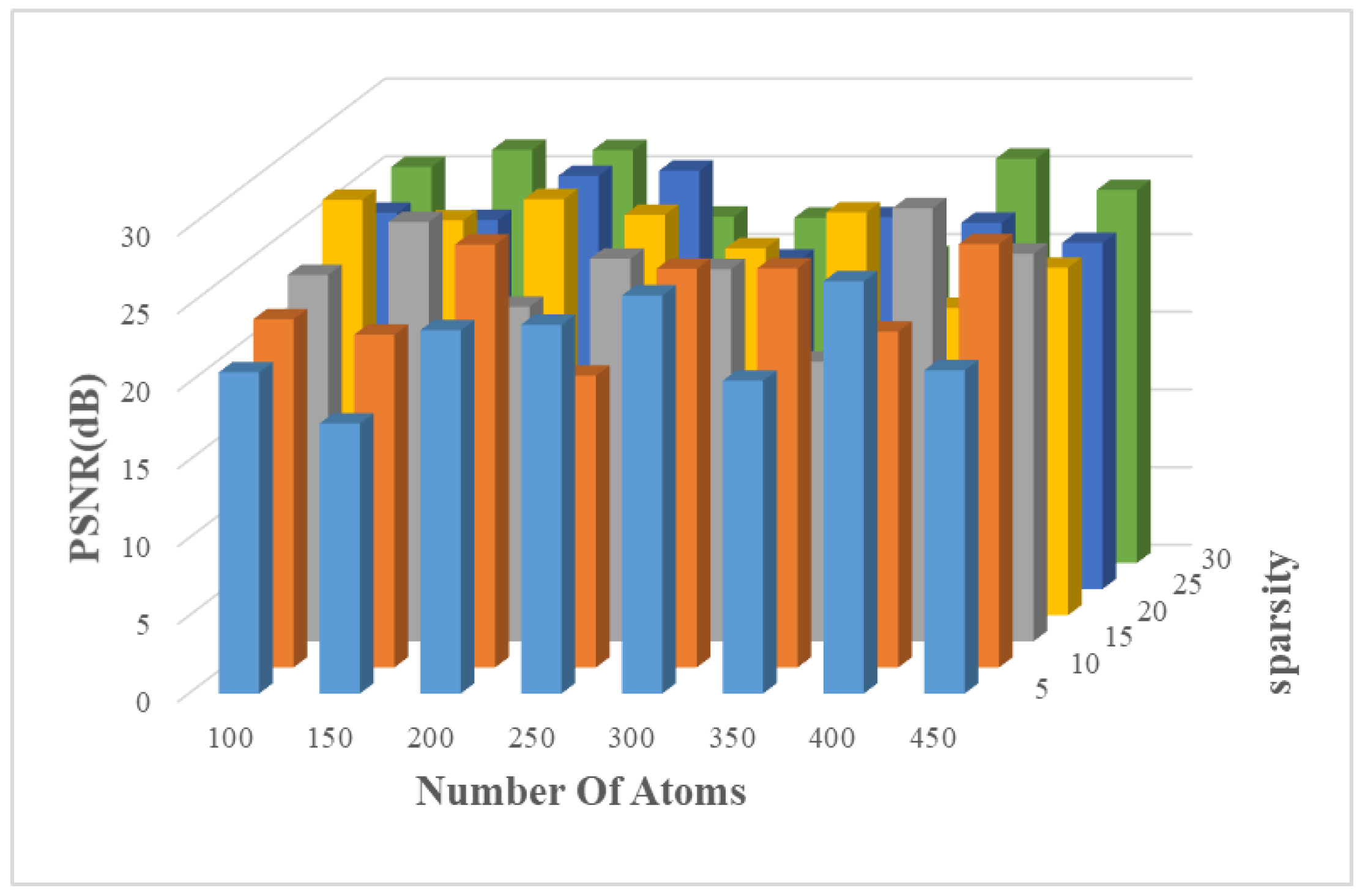
5.1.2. Dictionary Training

Knowing that the performance of the reconstruction result is highly dependent on the over-complete dictionary ${\mathcal{T}}_h$, the adopted datasets are all randomly divided into two parts according to a ratio of 1:1, including the training and test counterparts. In addition, 1000 samples are further selected as the final training set according to our proposed data preprocessing strategy. Moreover, experiments over the CAVE dataset are carried out to investigate the influence of different combinations of atoms and sparsities on the final reconstruction results. It can be observed from Figure 8 that the reconstruction quality does not vary too much, and the extremum appears around the value with the atoms set to 250 and sparsity set to 15, which is further adopted in our proposed method. It is worth noting that each combination experiment is repeated 5 times to alleviate the dictionary’s variation using the same training samples.

Figure 8. The influence of atoms and sparsity on the reconstruction performance over the CAVE dataset.

5.1.3. Sparse Reconstruction

After obtaining the hyperspectral dictionary $T_h$, the $T_h$ is then projected onto the RGB space through the $CIE\_1964$ color match function. In the process of generating the tensor RGB input, the neighboring pixels n should be odd. The number is then empirically set to 3 in this paper. As for the image edge, zero padding is adopted.

5.1.4. Experiment Metrics

Three reference quantitative metrics are introduced to evaluate the reconstruction performance from a spatial perspective, including the peak signal-to-noise ratio (PSNR), relative mean square error (RMSE) and structural similarity (SSIM) [48]. Note that all the datasets are linearly rescaled to [0,1] through normalization. Specifically, the PSNR metric is presented as follows:

$$PSNR(X,Y)=10{log}_{10}\left({\displaystyle \frac{Y_{max}}{MSE(X,Y)}}\right)$$

(22)

where $\mathit{X}$ is the reconstructed HSI, $\mathit{Y}$ is the reference HSI and ${\mathit{Y}}_{max}$ denotes the maximum value of all the pixels in one image. The MSE is the mean square error, presented as follows:

$$MSE(X,Y)=\frac{{\sum }_{i=1}^{n_1}{\sum }_{j=1}^{n_2}{\sum }_{z=1}^{n_3}{(X_{ijz}-Y_{ijz})}^2}{n_1\times n_2\times n_3}$$

(23)

where ${\mathit{n}}_{\mathit{1}}$ and ${\mathit{n}}_{\mathit{2}}$ are the spatial dimensions and ${\mathit{n}}_{\mathit{3}}$ denotes the number of spectral bands. In addition, the SSIM metric mainly computes the similarity of structure between two images, which is defined as follows:

$$SSIM(X,Y)={\displaystyle \frac{(2{\mu }_x{\mu }_y+c_1)(2{\sigma }_{xy}+c_2)}{({\mu }_x^2+{\mu }_y^2+c_1)({\sigma }_x^2+{\sigma }_y^2+c_2)}}$$

(24)

where $\sigma$ and $\mu$ are the average and variance of the HSI. ${\sigma }_{xy}$ is the covariance of $\mathit{X}$ and $\mathit{Y}$. ${\mathit{c}}_1={\left({\mathit{k}}_1\mathit{L}\right)}^2$, ${\mathit{c}}_2={\left({\mathit{k}}_2\mathit{L}\right)}^2$, ${\mathit{k}}_1=0.01$, ${\mathit{k}}_2=0.03$, and $\mathit{L}$ describes the dynamic range of the pixel values.

In addition to the spatial similarity, the spectral similarity is also vital to the reconstructed HSI. Therefore, the spectral angle mapper (SAM) is adopted to evaluate the similarity between two spectra through calculating the cosine distance, formulated as follows:

$$\theta =arccos{\displaystyle \frac{x_{(i,j)}·y_{(i,j)}}{\sqrt{{\sum }_{i=1}^{n_3}}x{(i,j)}^2·\sqrt{{\sum }_{i=1}^{n_3}}y{(i,j)}^2}}$$

(25)

where $\mathit{x}(\mathit{i},\mathit{j})$ and $\mathit{y}(\mathit{i},\mathit{j})$ represent the spectral bands at the position $(\mathit{i},\mathit{j})$.

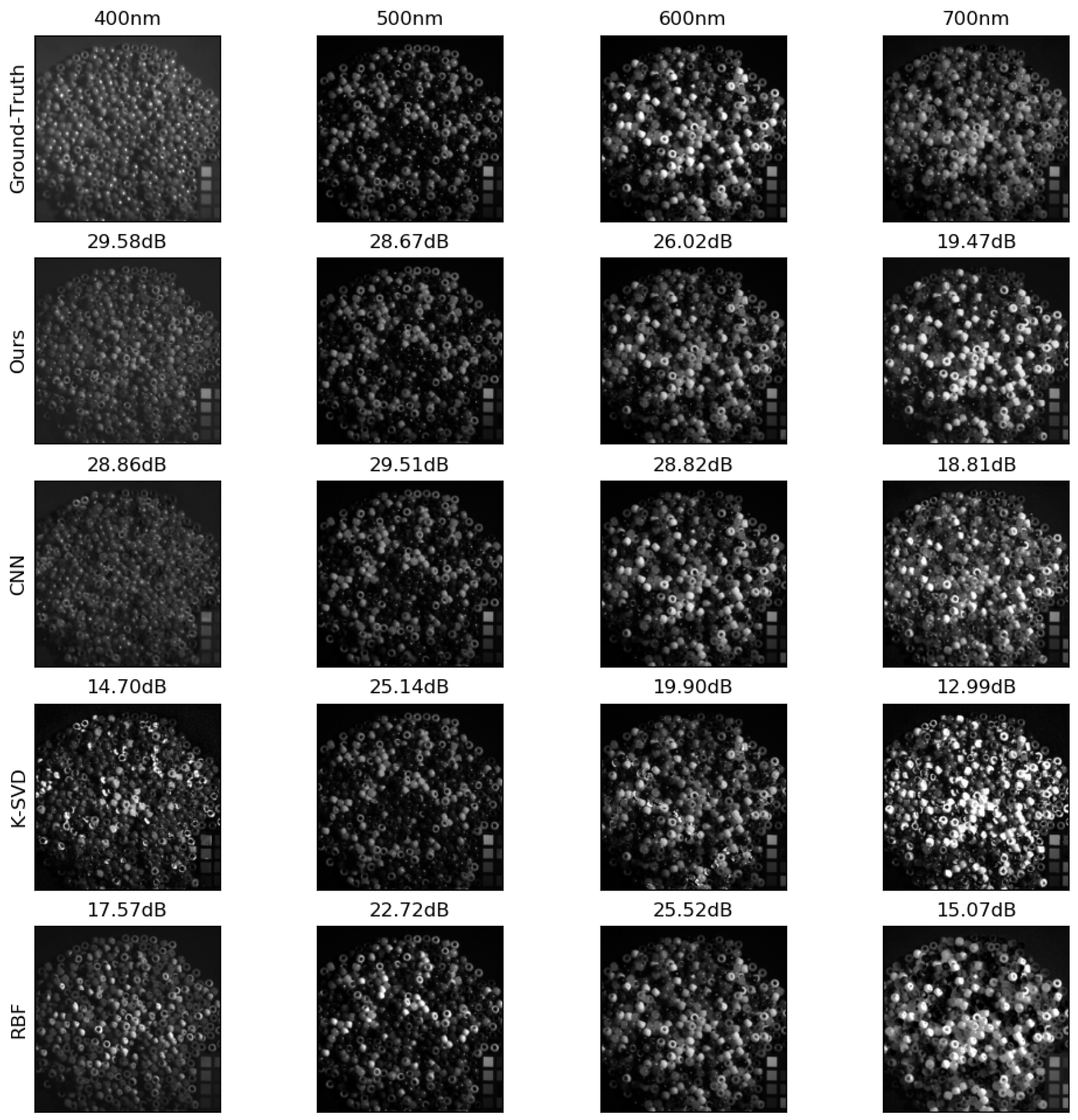
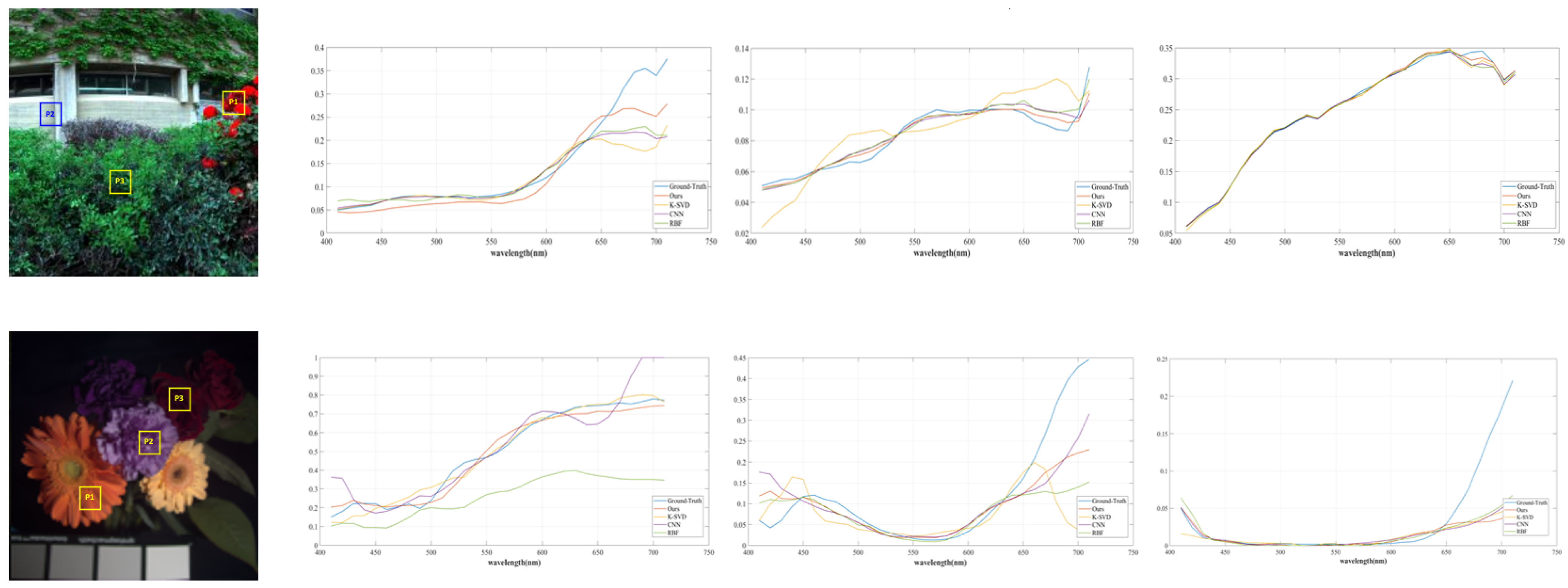
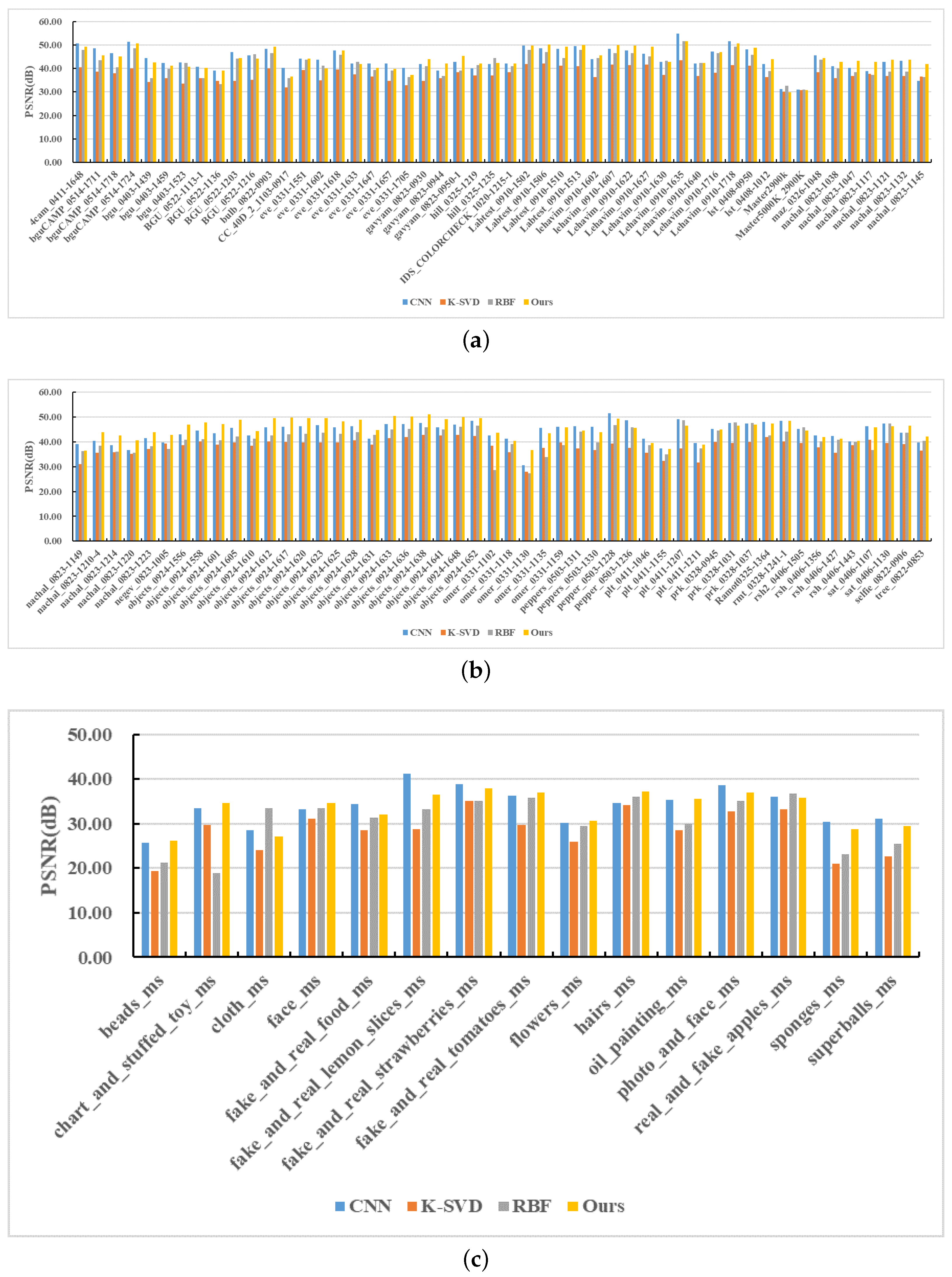
5.2. Quantitative and Qualitative Comparison Experiments

In this section, three classical approaches are introduced to make a comparison, including the K-SVD [21], RBF interpolation [22] and CNN [49], which are all evaluated on the ICVL and CAVE datasets under the same experimental settings. Table 2 gives the quantitative comparison of different methods in terms of the abovementioned terms, where the mean value of each metric and the standard variation are both tabulated. Moreover, the worst value of each metric for the different methods is also listed, including the largest RMSE and SAM and the smallest PSNR and SSIM. Notably, the bold form denotes the best result of each metric. As shown in Table 2, our proposed method obtains the best mean results in terms of the RMSE and PSNR over the ICVL dataset. As for the SSIM and SAM, our method is slightly worse than the CNN-based framework, which is acceptable. In the CAVE dataset, although our proposed method fails to achieve the best mean value of every metric, it is able to obtain the smallest standard variation in the PSNR, SSIM and SAM, which indicates a higher stability compared with the CNN-based method. In addition, compared with the CNN method, our proposed method has a more reasonable interpretability and less need of data while still being able to obtain comparable results.

Table 2. Quantitative results on ICVL and CAVE datasets. The bold values denote the best result for each metric.

	Methods	RMSE			PSNR			SSIM			SAM
		max	mean	std	min	mean	std	min	mean	std	max	mean	std
ICVL	K-SVD	0.0404	0.0136	0.0056	27.88	37.90	3.08	0.8804	0.9571	0.0194	0.2038	0.1030	0.0293
	RBF	0.0432	0.0097	0.0064	27.29	41.65	4.65	0.9130	0.9858	0.0112	0.1187	0.0485	0.0163
	CNN	0.0296	0.0072	0.0047	30.57	44.03	4.42	0.9653	0.9914	0.0063	0.1062	0.0397	0.0137
	Ours	0.0321	0.0067	0.0045	29.87	44.66	4.35	0.9679	0.9907	0.0062	0.1168	0.0407	0.0168
CAVE	K-SVD	0.1066	0.0445	0.0268	19.44	28.33	4.81	0.7481	0.9033	0.0630	0.5360	0.4216	0.0702
	RBF	0.1137	0.0373	0.0300	18.89	30.61	5.78	0.7536	0.9331	0.0585	0.4410	0.2660	0.0782
	CNN	0.0519	0.0226	0.0115	25.69	33.86	4.19	0.8815	0.9556	0.0268	0.3431	0.2017	0.0525
	Ours	0.0495	0.0238	0.0120	26.11	33.40	3.99	0.8973	0.9433	0.0191	0.3107	0.2217	0.0492

In addition, the individual results of each scene over two datasets in terms of the PSNR are also demonstrated in Figure 9. From those quantitative results, the conclusion can be drawn that the proposed method is able to reconstruct HSIs from RGB images with a consideriable quality.

Figure 9. (a,b) gives the ICVL reconstruction performance in terms of PSNR metric. (c) shows CAVE reconstruction performance over PSNR metric. The experiment uses 101 images of the ICVL dataset and 16 images of the CAVE dataset as the training images to construct the hyperspectral over-complete dictionary. The K-MEANS method is used to extract the training pixels.

In addition, qualitative comparison is further depicted in Figure 10 and Figure 11, where two scenes named “beads_ms” and “BGU_0403-1439” are selected from the CAVE and ICVL datasets, respectively. Four bands, 400 nm, 500 nm, 600 nm and 700 nm, are randomly chosen to demonstrate the reconstruction performance of the three methods and our proposed method, and the corresponding PSNR values are also listed above each subgraph. Obviously, our proposed method is capable of generating the target HSI that is the most visually similar to the ground truth. In addition, Figure 12 describes the spectral curve of the reconstruction HSIs, where three pixels are randomly selected from scenes “flowers_ms” and “PLT_04110-1046”. From the spectral curve analysis, our proposed method is able to recover the most similar curves with ground truth, confirming the applicability of our proposed framework.

Figure 10. Visual comparison of selected bands on scene “BGU_0403-1439” from ICVL dataset.

Figure 11. Visual comparison of selected bands on scene “beads_ms” from CAVE dataset.

Figure 12. Spectral curve analysis of random selected points (P1,P2 and P3) on two scenes. From top to bottom: “PLT_04110-1046” from ICVL dataset; “flowers_ms” from CAVE dataset.

6. Conclusions

In this paper, a novel tensor-based sparse representation for HSI reconstruction from RGB input is proposed, which exploits and integrates the spatial and spectral relations in a tensor-wise manner, avoiding breaking the original structure of input data during the SSR process. Firstly, the proposed framework preprocesses the training data to reduce the redundancy through introducing the K-MEANS method. On this basis, a more representative spectral dictionary can be trained through the preprocessed data. Then, the $CIE\_1964$ color match function is adopted to project the well-trained spectral dictionary onto the RGB space, after which the sparse coefficients of HSIs are able to be approximated through sparse solving in the RGB domain. After obtaining the sparse coefficients, the nonlinear mapping from RGB to HSI can be easily formulated. To further eliminate the spectral distortion, a spectral enhancement strategy based on MLP is proposed to promote the final performance. To this end, abundant experimental results over two public datasets demonstrate that the proposed framework can reconstruct HSIs with a high quality.

References

1. Campbell, J.B.; Wynne, R.H. Introduction to Remote Sensing; Guilford Press: New York, NY, USA, 2011. [Google Scholar]
2. Miao, C.; Pages, A.; Xu, Z.; Rodene, E.; Yang, J.; Schnable, J.C. Semantic segmentation of sorghum using hyperspectral data identifies genetic associations. Plant Phenomics 2020, 2020, 4216373. [Google Scholar] [CrossRef]
3. Lu, G.; Fei, B. Medical hyperspectral imaging: A review. J. Biomed. Opt. 2014, 19, 10901. [Google Scholar] [CrossRef] [PubMed]
4. Briottet, X.; Boucher, Y.; Dimmeler, A.; Malaplate, A.; Cini, A.; Diani, M.; Bekman, H.; Schwering, P.; Skauli, T.; Kasen, I.; et al. Military applications of hyperspectral imagery. In Targets and backgrounds XII: Characterization and Representation; SPIE: Bellingham, WA, USA, 2006; Volume 6239, pp. 82–89. [Google Scholar]
5. Stuart, M.B.; McGonigle, A.J.; Willmott, J.R. Hyperspectral imaging in environmental monitoring: A review of recent developments and technological advances in compact field deployable systems. Sensors 2019, 19, 3071. [Google Scholar] [CrossRef]
6. Manolakis, D.; Shaw, G. Detection algorithms for hyperspectral imaging applications. IEEE Signal Process. Mag. 2002, 19, 29–43. [Google Scholar] [CrossRef]
7. Treado, P.; Nelson, M.; Gardner, C., Jr. Hyperspectral Imaging Sensor for Tracking Moving Targets. U.S. Patent 13/199,981, 15 March 2012. [Google Scholar]
8. Nguyen, H.V.; Banerjee, A.; Chellappa, R. Tracking via object reflectance using a hyperspectral video camera. In Proceedings of the 2010 IEEE Computer Society Conference on Computer Vision and Pattern Recognition-Workshops, San Francisco, CA, USA, 13–18 June 2010; pp. 44–51. [Google Scholar]
9. Chen, Y.; Lin, Z.; Zhao, X.; Wang, G.; Gu, Y. Deep learning-based classification of hyperspectral data. IEEE J. Sel. Top. Appl. Earth Obs. Remote Sens. 2014, 7, 2094–2107. [Google Scholar] [CrossRef]
10. Chang, C.-I. Hyperspectral Imaging: Techniques for Spectral Detection and Classification; Springer Science & Business Media: Berlin/Heidelberg, Germany, 2003; Volume 1. [Google Scholar]
11. Mei, S.; Ji, J.; Hou, J.; Li, X.; Du, Q. Learning sensor-specific spatial-spectral features of hyperspectral images via convolutional neural networks. IEEE Trans. Geosci. Remote Sens. 2017, 55, 4520–4533. [Google Scholar] [CrossRef]
12. Mei, S.; Song, C.; Ma, M.; Xu, F. Hyperspectral image classification using group-aware hierarchical transformer. IEEE Trans. Geosci. Remote Sens. 2022, 60, 1–14. [Google Scholar] [CrossRef]
13. Lian, J.; Mei, S.; Zhang, S.; Ma, M. Benchmarking adversarial patch against aerial detection. IEEE Trans. Geosci. Remote Sens. 2022, 60, 1–16. [Google Scholar] [CrossRef]
14. Mei, S.; Jiang, R.; Ma, M.; Song, C. Rotation-invariant feature learning via convolutional neural network with cyclic polar coordinates convolutional layer. IEEE Trans. Geosci. Remote Sens. 2023, 61, 1–13. [Google Scholar] [CrossRef]
15. Liu, Y.; Zhang, Y.; Wang, Y.; Mei, S. Rethinking transformers for semantic segmentation of remote sensing images. IEEE Trans. Geosci. Remote Sens. 2023, 61, 5617515. [Google Scholar] [CrossRef]
16. ElMasry, G.; Sun, D.-W. Principles of hyperspectral imaging technology. In Hyperspectral Imaging for Food Quality Analysis and Control; Elsevier: Amsterdam, The Netherlands, 2010; pp. 3–43. [Google Scholar]
17. Wei, Q.; Bioucas-Dias, J.; Dobigeon, N.; Tourneret, J.-Y. Hyperspectral and multispectral image fusion based on a sparse representation. IEEE Trans. Geosci. Remote Sens. 2015, 53, 3658–3668. [Google Scholar] [CrossRef]
18. Liu, Y.; Wang, Z. Multi-focus image fusion based on sparse representation with adaptive sparse domain selection. In Proceedings of the 2013 Seventh International Conference on Image and Graphics, Qingdao, China, 26–28 July 2013; pp. 591–596. [Google Scholar]
19. Ma, X.; Hu, S.; Liu, S.; Fang, J.; Xu, S. Remote sensing image fusion based on sparse representation and guided filtering. Electronics 2019, 8, 303. [Google Scholar] [CrossRef]
20. Xia, K.-J.; Yin, H.-S.; Wang, J.-Q. A novel improved deep convolutional neural network model for medical image fusion. Clust. Comput. 2019, 22, 1515–1527. [Google Scholar] [CrossRef]
21. Arad, B.; Ben-Shahar, O. Sparse recovery of hyperspectral signal from natural rgb images. In Proceedings of the Computer Vision–ECCV 2016: 14th European Conference, Amsterdam, The Netherlands, 11–14 October 2016; Proceedings, Part VII 14. Springer: Berlin/Heidelberg, Germany, 2016; pp. 19–34. [Google Scholar]
22. Nguyen, R.M.; Prasad, D.K.; Brown, M.S. Training-based spectral reconstruction from a single rgb image. In Proceedings of the Computer Vision–ECCV 2014: 13th European Conference, Zurich, Switzerland, 6–12 September 2014; Proceedings, Part VII 13. Springer: Berlin/Heidelberg, Germany, 2014; pp. 186–201. [Google Scholar]
23. Aeschbacher, J.; Wu, J.; Timofte, R. In defense of shallow learned spectral reconstruction from rgb images. In Proceedings of the IEEE International Conference on Computer Vision Workshops, Venice, Italy, 22–29 October 2017; pp. 471–479. [Google Scholar]
24. Stiebel, T.; Koppers, S.; Seltsam, P.; Merhof, D. Reconstructing spectral images from rgb-images using a convolutional neural network. In Proceedings of the IEEE Conference on Computer Vision and Pattern Recognition Workshops, Salt Lake City, UT, USA, 18–23 June 2018; pp. 948–953. [Google Scholar]
25. Stigell, P.; Miyata, K.; Hauta-Kasari, M. Wiener estimation method in estimating of spectral reflectance from rgb images. Pattern Recognit. Image Anal. 2007, 17, 233–242. [Google Scholar] [CrossRef]
26. Yan, Y.; Zhang, L.; Li, J.; Wei, W.; Zhang, Y. Accurate spectral super-resolution from single rgb image using multi-scale cnn. In Proceedings of the Pattern Recognition and Computer Vision: First Chinese Conference, PRCV 2018, Guangzhou, China, 23–26 November 2018; Proceedings, Part II 1. Springer: Berlin/Heidelberg, Germany, 2018; pp. 206–217. [Google Scholar]
27. Banerjee, A.; Palrecha, A. Mxr-u-nets for real time hyperspectral reconstruction. arXiv 2020, arXiv:2004.07003. [Google Scholar]
28. Zhao, Y.; Po, L.-M.; Yan, Q.; Liu, W.; Lin, T. Hierarchical regression network for spectral reconstruction from rgb images. In Proceedings of the IEEE/CVF Conference on Computer Vision and Pattern Recognition Workshops, Seattle, WA, USA, 14–19 June 2020; pp. 422–423. [Google Scholar]
29. Xiong, Z.; Shi, Z.; Li, H.; Wang, L.; Liu, D.; Wu, F. Hscnn: Cnn-based hyperspectral image recovery from spectrally undersampled projections. In Proceedings of the IEEE International Conference on Computer Vision Workshop, Venice, Italy, 22–29 October 2017; pp. 518–525. [Google Scholar]
30. Koundinya, S.; Sharma, H.; Sharma, M.; Upadhyay, A.; Manekar, R.; Mukhopadhyay, R.; Karmakar, A.; Chaudhury, S. 2d-3d cnn based architectures for spectral reconstruction from rgb images. In Proceedings of the IEEE Conference on Computer Vision and Pattern Recognition Workshops, Salt Lake City, UT, USA, 18–22 June 2018; pp. 844–851. [Google Scholar]
31. Li, J.; Wu, C.; Song, R.; Xie, W.; Ge, C.; Li, B.; Li, Y. Hybrid 2-d–3-d deep residual attentional network with structure tensor constraints for spectral super-resolution of rgb images. IEEE Trans. Geosci. Remote Sens. 2020, 59, 2321–2335. [Google Scholar] [CrossRef]
32. Peng, H.; Chen, X.; Zhao, J. Residual pixel attention network for spectral reconstruction from rgb images. In Proceedings of the IEEE/CVF Conference on Computer Vision and Pattern Recognition Workshops, Seattle, WA, USA, 14–19 June 2020; pp. 486–487. [Google Scholar]
33. Yi, C.; Zhao, Y.-Q.; Chan, J.C.-W. Spectral super-resolution for multispectral image based on spectral improvement strategy and spatial preservation strategy. IEEE Trans. Geosci. Remote Sens. 2019, 57, 9010–9024. [Google Scholar] [CrossRef]
34. Timofte, R.; Smet, V.D.; Gool, L.V. A+: Adjusted anchored neighborhood regression for fast super-resolution. In Proceedings of the Computer Vision–ACCV 2014: 12th Asian Conference on Computer Vision, Singapore, 1–5 November 2014; Revised Selected Papers, Part IV 12. Springer: Berlin/Heidelberg, Germany, 2015; pp. 111–126. [Google Scholar]
35. Mei, S.; Geng, Y.; Hou, J.; Du, Q. Learning hyperspectral images from rgb images via a coarse-to-fine cnn. Sci. China Inf. Sci. 2022, 65, 1–14. [Google Scholar] [CrossRef]
36. Mei, S.; Zhang, G.; Wang, N.; Wu, B.; Ma, M.; Zhang, Y.; Feng, Y. Lightweight multiresolution feature fusion network for spectral super-resolution. IEEE Trans. Geosci. Remote Sens. 2023, 61, 1–14. [Google Scholar] [CrossRef]
37. Chakrabarti, A.; Zickler, T. Statistics of real-world hyperspectral images. In Proceedings of the 2011 IEEE Conference on Computer Vision and Pattern Recognition, Washington, DC, USA, 20–25 June 2011; pp. 193–200. [Google Scholar]
38. Peng, J.; Huang, Y.; Sun, W.; Chen, N.; Ning, Y.; Du, Q. Domain adaptation in remote sensing image classification: A survey. IEEE J. Sel. Top. Appl. Earth Obs. Remote Sens. 2022, 15, 9842–9859. [Google Scholar] [CrossRef]
39. Huang, Y.; Peng, J.; Sun, W.; Chen, N.; Du, Q.; Ning, Y.; Su, H. Two-branch attention adversarial domain adaptation network for hyperspectral image classification. IEEE Trans. Geosci. Remote Sens. 2022, 60, 1–13. [Google Scholar] [CrossRef]
40. Huang, Y.; Peng, J.; Chen, N.; Sun, W.; Du, Q.; Ren, K.; Huang, K. Cross-scene wetland mapping on hyperspectral remote sensing images using adversarial domain adaptation network. ISPRS J. Photogramm. Remote Sens. 2023, 203, 37–54. [Google Scholar] [CrossRef]
41. Tominaga, S.; Wandell, B.A. Standard surface-reflectance model and illuminant estimation. JOSA A 1989, 6, 576–584. [Google Scholar] [CrossRef]
42. Geng, Y.; Mei, S.; Tian, J.; Zhang, Y.; Du, Q. Spatial constrained hyperspectral reconstruction from rgb inputs using dictionary representation. In Proceedings of the IGARSS 2019–2019 IEEE International Geoscience and Remote Sensing Symposium, Yokohama, Japan, 28 July–2 August 2019; pp. 3169–3172. [Google Scholar]
43. Kolda, T.G.; Bader, B.W. Tensor decompositions and applications. SIAM Rev. 2009, 51, 455–500. [Google Scholar] [CrossRef]
44. Bader, B.W.; Kolda, T.G. Algorithm 862: Matlab tensor classes for fast algorithm prototyping. ACM Trans. Math. Softw. (TOMS) 2006, 32, 635–653. [Google Scholar] [CrossRef]
45. Hartigan, J.A.; Wong, M.A. Algorithm as 136: A k-means clustering algorithm. J. R. Stat. Soc. Ser. C (Appl. Stat.) 1979, 28, 100–108. [Google Scholar] [CrossRef]
46. Aharon, M.; Elad, M.; Bruckstein, A. K-svd: An algorithm for designing overcomplete dictionaries for sparse representation. IEEE Trans. Signal Process. 2006, 54, 4311–4322. [Google Scholar] [CrossRef]
47. Yasuma, F.; Mitsunaga, T.; Iso, D.; Nayar, S.K. Generalized assorted pixel camera: Postcapture control of resolution, dynamic range, and spectrum. IEEE Trans. Image Process. 2010, 19, 2241–2253. [Google Scholar] [CrossRef]
48. Wang, Z.; Bovik, A.C.; Sheikh, H.R.; Simoncelli, E.P. Image quality assessment: From error visibility to structural similarity. IEEE Trans. Image Process. 2004, 13, 600–612. [Google Scholar] [CrossRef]
49. Arad, B.; Ben-Shahar, O.; Timofte, R.; Gool, L.V.; Zhang, L.; Yang, M. Ntire 2018 challenge on spectral reconstruction from rgb images. In Proceedings of the 2018 IEEE/CVF Conference on Computer Vision and Pattern Recognition Workshops (CVPRW), Salt Lake City, UT, USA, 18–22 June 2018; p. 1042. [Google Scholar]
Disclaimer/Publisher’s Note: The statements, opinions and data contained in all publications are solely those of the individual author(s) and contributor(s) and not of MDPI and/or the editor(s). MDPI and/or the editor(s) disclaim responsibility for any injury to people or property resulting from any ideas, methods, instructions or products referred to in the content.
Article Metrics
Citations
Article Access Statistics
Multiple requests from the same IP address are counted as one view.