Analysis of Block Adaptive Type-II Progressive Hybrid Censoring with Weibull Distribution

Abstract

The estimation of unknown model parameters and reliability characteristics is considered under a block adaptive progressive hybrid censoring scheme, where data are observed from a Weibull model. This censoring scheme enhances experimental efficiency by conducting experiments across different testing facilities. Point and interval estimates for parameters and reliability assessments are derived using both classical and Bayesian approaches. The existence and uniqueness of maximum likelihood estimates are established. Consequently, reliability performance and differences across different testing facilities are analyzed. In addition, a Metropolis–Hastings sampling algorithm is developed to approximate complex posterior computations. Approximate confidence intervals and highest posterior density credible intervals are obtained for the parametric functions. The performance of all estimators is evaluated through an extensive simulation study, and observations are discussed. A cancer dataset is analyzed to illustrate the findings under the block adaptive censoring scheme.

1. Introduction

Censoring is frequently used in lifetime experiments to address cost and time constraints, especially when testing modern reliable products that require long testing cycles in traditional experiments. In practical scenarios, various censoring schemes are implemented with different objectives to enhance efficiency and reduce unnecessary expenses. Censoring is common in fields such as industrial engineering (e.g., reliability engineering, machine operations, radio inferences), clinical trials, and biological experiments. Among the most conventional methods are type-I and type-II censoring schemes, where tests are terminated at a fixed time point T or at the m-th failure, respectively. The mixture of these two conventional censoring schemes is referred to as a hybrid censoring scheme. These methods do not permit the removal of experimental units at intermediate stages. To address this limitation, the progressive type-II censoring scheme, introduced by Cohen [1], allows the removal of units at different stages of an experiment. Since then, many researchers have analyzed this scheme under various contexts. Balakrishnan and Sandhu [2] proposed algorithms to generate samples from this scheme. For a comprehensive review, one can refer to the monographs of Balakrishnan and Aggarwala [3] and Balakrishnan and Cramer [4]. Wang [5], Chandra et al. [6] and Lodhi et al. [7] obtained results for progressively censored competing risks data. Singh et al. [8,9] and Mahto et al. [10] discuss estimation under multicomponent stress–strength model when data are progressive censored. Almetwally et al. [11], El-Sherpieny et al. [12], Maurya et al. [13], Lodhi et al. [14] further describe important results under this scheme.

Kundu and Joarder [15] combined progressive type-II censoring and hybrid censoring schemes and obtained a progressive type-II hybrid censoring scheme. This scheme is useful in improving the efficacy of an experiment. Here, an experiment stops at time point $min(X_m,T)$, where $X_m$ represents the time of m-th failure and T is a pre-fixed experimental time. It has some interesting features as well. For instance, the effective sample size may be uncertain and possibly very small, which can affect the efficiency of proposed inference. Thus, a more flexible censoring scheme may be required in such studies. Ng et al. [16] introduced an adaptive type-II progressive hybrid censoring scheme (AII-PHCS), where experimental time may exceed the predetermined time T and the effective sample size m remains prefixed. In AII-PHCS, n identical units are put on the experiment, number of failures to be observed is $m(\le n)$ and a progressive scheme $(R_1,R_2,\dots ,R_m)$, where $R_m=n-m-{\sum }_{i=1}^{m-1}{R}_i$. Consider $X_i(i=1,2,\dots ,m)$ represents the failure time of i-th unit. Let $(X_1,X_2,\dots ,X_m)$ be a progressive type-II censored data. During AII-PHCS, if $X_m<T$, then the test ends at $X_m$, which is just the usual progressive type-II censoring process. Otherwise, if $X_J<T<X_{J+1}$, here $(J=1,2,\dots ,m-1)$, then we set $R_{J+1}=R_{J+2}=\cdots =R_{m-1}=0$ and $R_m=n-m-{\sum }_{j=1}^J{R}_j$ to adjust the removal scheme. During the AII-PHCS procedure, the censoring scheme $(R_1,R_2,\dots ,R_m)$ changes to $(R_1,R_2,\dots ,R_J,0,\dots ,0,R_m^{*})$ and $R_m^{*}=n-m-{\sum }_{j=1}^J{R}_j$. This adaptation ensures that the experiment will end once the predetermined number of failures has been obtained. Recently, this censoring has gained considerable attention among researchers. For comprehensive discusions, see Nassar and Kasem [17], Dutta et al. [18], Elshahhat et al. [19], Gangopadhyay et al. [20]. Nassar et al. [21] derived estimates for Weibull parameters under the AII-PHCS scheme. Additionally, Ren and Gui [22,23] discussed Bayesian estimation for competing risks data under AII-PHCS, while Almetwally et al. [24,25] obtained parameter estimates of some known distributions using the maximum product spacing technique.

At times, it may not be feasible to monitor each subject under study simultaneously. Such situations may arise due to factors such as the unavailability or difficulty of accessing the equipment required to conduct life tests on all units simultaneously. Ahmadi et al. [26] recently introduced a more flexible testing approach known as the block censoring scheme, which can enhance test efficiency. This scheme is implemented as follows: suppose there are $n_i(i=1,2,\dots ,m)$ units in the i-th group of m groups formed from n identical test units. Furthermore, m facilities are employed to test all m groups under type-II censoring conditions. As it can be challenging for an experimenter to inspect every unit concurrently, a block censoring scheme may provide a more realistic testing framework. Accordingly, testing of units can be conducted in various groups in a more adaptable and efficient manner. For a detailed discussion on the block censoring scheme, readers are referred to Zhu [27].

The block censoring scheme involves conducting lifetime experiments across different testing groups under type-II censoring. However, advancements in manufacturing processes often result in products with extended life cycles and high reliability, making it challenging to collect an adequate number of failures under type-II censoring. To address this, Kumari et al. [28,29] introduced a novel censoring approach known as the block progressive type-II censoring scheme, which offers enhanced flexibility and efficiency. Under this scheme, units are tested in different groups using different testing facilities to minimize the experimentation duration. While testing facilities are generally assumed to be identical, in practice, failure times collected from different testing facilities may not be completely uniform. Differences may arise due to various factors, including operating conditions, personnel testing specifications, environmental conditions, and data collection accuracy. Consequently, it is more appropriate to consider such data as non-identical records, with substantial implications of differences across different facilities (DDF) as significant consequences. Wang et al. [30] obtained classical and hierarchical Bayesian estimates of parametric quantities when data follow an inverted exponentiated exponential distribution. However, limited research has been conducted on the block adaptive type-II hybrid progressive censoring scheme (BAII-PHCS). In this paper, we derive point and interval estimates for model parameters and reliability indices under the BAII-PHCS framework. These estimates specifically include reliability and failure rate functions, utilizing both maximum likelihood estimation (MLE) and hierarchical Bayesian approaches.

The objective of this study is to derive various estimates for parameters and reliability characteristics of the Weibull model based on the BAII-PHCS scheme. Suppose X is a random variable following a Weibull distribution. The probability density function (PDF) and cumulative distribution function (CDF) of X are, respectively, given as follows

$$\begin{array}{c}\hfill f(x;\alpha ,\beta )=\alpha \beta x^{\alpha -1}exp\left\{-\beta x^{\alpha }\right\},x>0,\end{array}$$

(1)

and

$$\begin{array}{c}\hfill F(x;\alpha ,\beta )=1-exp\left\{-\beta x^{\alpha }\right\},x>0,\end{array}$$

where $\alpha >0$ and $\beta >0$ are shape and scale parameters, respectively. Furthermore, the survival function (SF) $S(·)$, hazard rate function (HRF) $H(·)$ and the mean time to failure (MTF) of the Weibull model are expressed as

$$S(x;\alpha ,\beta )=exp\left\{-\beta x^{\alpha }\right\},$$

$$H(x;\alpha ,\beta )=\alpha \beta x^{\alpha -1},$$

and

$$MTF(\alpha ,\beta )={\beta }^{-1/\alpha }\mathsf{\Gamma }\left((1/\alpha )+1\right).$$

The Weibull distribution is widely utilized in reliability and lifetime studies. Notably, the commonly used exponential and Rayleigh distributions are special cases of the Weibull distribution. Weibull [31] describe several important properties of this model. A vast array of references on the Weibull model is available, underscoring its importance in this field. Several extensions of the Weibull distribution have been introduced and studied in the literature to analyze a broad range of lifetime data. For a detailed discussion, see Murthy et al. [32]. Additionally, Lai et al. [33] present several valuable extensions of the Weibull distribution that are particularly useful in lifetime analysis.

In Section 2, we present the model description and describe the likelihood function under the BAII-PHCS scheme. Section 3 outlines the derivation of maximum likelihood estimators for the unknown parameters, reliability characteristics, and DDF. Section 4 discusses Bayesian point and credible interval estimates for the proposed model. The effectiveness of all studied estimators is assessed through an extensive simulation study in Section 5. Furthermore, a real dataset is analyzed for illustration purposes. Concluding remarks are provided in Section 6.

2. Model Description

Data Description and Testing Methodology

Assume that k groups and n identical units are tested under BAII-PHCS with fixed experiment time T. Under the AII-PHCS scheme, every group of size $n_i,i=1,2,\dots ,k$ is put to the test, where ${\sum }_{i=1}^k{n}_i=n$. Assume that in the i-th group, the effective number of observed failures is $m_i$ and experimental time being $T_i(i=1,2,\dots ,k)$. In the i-th testing group, the prefixed censoring scheme is ${\mathcal{R}}_i=(R_{i1},R_{i2},\dots ,R_{i{m}_i})$. Consider that the time of i-th failure of units is represented as $X_{i{m}_i}$. In BAII-PHCS, if $X_{i{m}_i}<T_i$ then the experiment is terminated at $X_{i{m}_i}$ with the censoring scheme being $(R_{i1},R_{i2},\dots ,R_{i{m}_i}=n_i-m_i-{\sum }_{j=1}^{m_i-1}{R}_{ij})$ for i-th testing group. Otherwise, if $X_{i{m}_i}>T_i$, then there exists $J_i$ such that $X_{i{J}_i}<T_i<X_{i{J}_i+1}$ and the experiment terminates at $X_{i{m}_i}$ with no removal by setting $R_{i\ell }=0$, where $\ell =J_i+1,\dots ,m_i-1$ and $R_{i{m}_i}=n_i-m_i-{\sum }_{j=1}^{J_i}{R}_{ij}$. In BAII-PHCS, the censoring scheme $(R_{i1},R_{i2},\dots ,R_{i{m}_i})$ becomes $(R_{i1},R_{i2},\dots ,R_{i{J}_i},0,\dots ,0,R_{i{m}_i}^{*}=n_i-m_i-{\sum }_{j=1}^{J_i}{R}_{ij})$ for each i-th group.

Following the AII-PHCS scheme, the failure times under i-th group are observed as ${\mathcal{X}}_i=(X_{i1},X_{i2},\dots ,X_{i{m}_i})$. Assume that products’ lifetimes follow a Weibull distribution with $\alpha$ and ${\beta }_i$ being parameters. By taking DDF into consideration, lifetimes of units under i-th group with i-th testing facility is considered to have a Weibull model with parameters $\alpha$ and ${\beta }_i$. The PDF and CDF are given as

$$\begin{array}{cc}\hfill f(x;\alpha ,{\beta }_i)=& \alpha {\beta }_i{x}^{\alpha -1}exp\left(-\beta x^{\alpha }\right),x>0,\alpha ,{\beta }_i>0,\hfill \\ \hfill F(x;\alpha ,{\beta }_i)=& 1-exp\left(-{\beta }_i{x}^{\alpha }\right).\hfill \end{array}$$

The failure times are obtained under BAII-PHCS, as follows:

Group	Data id	Detailed samples
1	${\mathcal{G}}_1^{\prime }$	$\left\{\begin{array}{c}\mathrm{Case}\text{-}\mathrm{I}:(x_{11},R_{11}),(x_{12},R_{12}),\dots ,(x_{1m_1},R_{1m_1}),if{X}_{1m_1}<T_1\hfill \\ \mathrm{Case}\text{-}\mathrm{II}:(x_{11},R_{11}),(x_{12},R_{12}),\dots ,(x_{1J_1},R_{1J_1}),\hfill \\ (x_{1J_1+1},0),\dots ,(x_{1m_1-1},0),(x_{1m_1},R_{1m_1}^{*})if{X}_{1m_1}>T_1\hfill \end{array}\right.$
2	${\mathcal{G}}_2^{\prime }$	$\left\{\begin{array}{c}\mathrm{Case}\text{-}\mathrm{I}:(x_{21},R_{21}),(x_{22},R_{22}),\dots ,(x_{2m_2},R_{2m_2}),if{X}_{2m_2}<T_2\hfill \\ \mathrm{Case}\text{-}\mathrm{II}:(x_{21},R_{21}),(x_{22},R_{22}),\dots ,(x_{2J_2},R_{2J_2}),\hfill \\ (x_{2J_2+1},0),\dots ,(x_{2m_2-1},0),(x_{2m_2},R_{2m_2}^{*}),if{X}_{2m_2}>T_2\hfill \end{array}\right.$
⋮	⋮	⋮
k	${\mathcal{G}}_k^{\prime }$	$\left\{\begin{array}{c}\mathrm{Case}\text{-}\mathrm{I}:(x_{k1},R_{k1}),(x_{k2},R_{k2}),\dots ,(x_{k{m}_k},R_{k{m}_k}),if{X}_{k{m}_k}<T_k\hfill \\ \mathrm{Case}\text{-}\mathrm{II}:(x_{k1},R_{k1}),(x_{k2},R_{k2}),\dots ,(x_{k{J}_k},R_{k{J}_k}),\hfill \\ (x_{k{J}_k+1},0),\dots ,(x_{k{m}_k-1},0),(x_{k{m}_k},R_{k{m}_k}^{*}),if{X}_{k{m}_k}>T_k.\hfill \end{array}\right.$

It is worth noting that different facilities might possess similar inherent operating mechanisms. Thus, we utilize common parameter $\alpha$ across these facilities as a presumed reflection of such influence. However, distinct parameters ${\beta }_1,{\beta }_2,\dots ,{\beta }_k$ are also incorporated to address the facility effect within the k testing groups. These parameters encapsulate the variability in testing identical units across test facilities. Essentially, the discrepancies in different ${\beta }_i$ contribute to the DDF, and precise estimation of these quantities is vital for overall adequate estimation of DDF function. Moreover, considering that DDF may not be neglected, the parameter $\beta$ in (1) can be estimated through a weighted estimation of ${\beta }_i$ in following manner:

$$\beta ={\displaystyle \frac{{\sum }_{i=1}^k{\eta }_i{\beta }_i}{{\sum }_{i=1}^k{\eta }_i}}.$$

Here, ${\eta }_i(i=1,2,\dots ,k)$ denotes the weight coefficient, and ${\eta }_i={\displaystyle \frac{1}{Var\left({\beta }_i\right)}}$, where $Var\left({\beta }_i\right)$ stands for the variance of ${\beta }_i$, which is defined in following section.

3. Maximum Likelihood Estimation

Under BAII-PHCS data described above, suppose that failure times ${\mathcal{G}}_i^{\prime },i=1,2,\dots ,k,$ represent AII-PHCS samples from the Weibull distribution with parameters $\alpha$ and ${\beta }_i$ in the i-th testing group. Then corresponding likelihood function is formulated as:

$$\begin{array}{cc}\hfill L_i(\alpha ,{\beta }_i;{\mathcal{G}}_i^{\prime })=& C_i\prod _{j=1}^{m_i}f(x_{ij};\alpha ,{\beta }_i)\times \prod _{j=1}^{J_i}{\left[1-F(x_{ij};\alpha ,{\beta }_i)\right]}^{R_{ij}}\times {\left[1-F(x_{i{m}_i};\alpha ,{\beta }_i)\right]}^{R_{i{m}_i}^{*}},\hfill \\ \hfill \propto & {\alpha }^{m_i}\times {\beta }_i^{m_i}\times \prod _{j=1}^{m_i}{x}_{ij}^{\alpha }\times exp\left\{-{\beta }_i\left(\sum _{j=1}^{m_i}{x}_{ij}^{\alpha }+\sum _{j=1}^{J_i}{x}_{ij}^{\alpha }{R}_{ij}+x_{i{m}_i}^{\alpha }{R}_{i{m}_i}^{*}\right)\right\},\hfill \end{array}$$

where $C_i={\prod }_{j=1}^{m_i}\left(n_i-j+1-{\sum }_{l=1}^{min(j-1,J_i)}{R}_{il}\right)$ is the normalizing constant.

Consider $\mathcal{G}=({\mathcal{G}}_1^{\prime },{\mathcal{G}}_2^{\prime },\dots ,{\mathcal{G}}_m^{\prime })$ and $\mathcal{B}=({\beta }_1,{\beta }_2,\dots ,{\beta }_k)$, now full likelihood function of $\alpha$ and $\mathcal{B}$ becomes

$$\begin{array}{cc}\hfill L(\alpha ,\mathcal{B};{\mathcal{G}}^{\prime })=& \prod _{i=1}^k{L}_i(\alpha ,{\beta }_i;{\mathcal{G}}_i^{\prime })\hfill \\ \hfill =& {\alpha }^{{\sum }_{i=1}^k{m}_i}\times \prod _{i=1}^k{\beta }_i^{m_i}\times \prod _{i=1}^k\prod _{j=1}^{m_i}{x}_{ij}^{\alpha -1}\times exp\left\{-\sum _{i=1}^k{\beta }_i{\mathsf{\Psi }}_i\left(\alpha \right)\right\},\hfill \end{array}$$

(2)

where ${\mathsf{\Psi }}_i\left(\alpha \right)={\sum }_{j=1}^{m_i}{x}_{ij}^{\alpha }+{\sum }_{j=1}^{J_i}{x}_{ij}^{\alpha }{R}_{ij}+x_{i{m}_i}^{\alpha }{R}_{i{m}_i}^{*}$.

From (2), the associated log-likelihood function of $\alpha$ and $\mathcal{B}$ is written as

$$\begin{array}{c}\hfill \ell (\alpha ,\mathcal{B};{\mathcal{G}}^{\prime })=ln\alpha \sum _{i=1}^k{m}_i+\sum _{i=1}^k{m}_{i}ln{\beta }_i+(\alpha -1)\sum _{i=1}^k\sum _{j=1}^{m_i}ln{x}_{ij}-\sum _{i=1}^k{\beta }_i{\mathsf{\Psi }}_i\left(\alpha \right).\end{array}$$

(3)

As a result, the MLEs of $\alpha$ and ${\beta }_i,i=1,2,\dots ,k$, denoted as $\widehat{\alpha }$ and $\widehat{\mathcal{B}}=({\widehat{\beta }}_1,{\widehat{\beta }}_2,\dots ,{\widehat{\beta }}_k)$, respectively, are obtained as solutions of the following likelihood Equation (3)

$$\begin{array}{c}\hfill {\ell }_{\alpha }=0\mathrm{and}{\ell }_{{\beta }_1}=0,{\ell }_{{\beta }_2}=0,\cdots ,{\ell }_{{\beta }_k}=0,\end{array}$$

(4)

where ${\ell }_{(·)}$ denotes the first derivative of $\ell (\alpha ,\mathcal{B};\mathcal{G})$ with respect to the associated parameters. We omit the details to save space. We can use Newton–Raphson or quasi-Newton methods to solve the likelihood Equation (4). However, we propose an alternative approach involving the profile log-likelihood function. The estimators that maximize profile log-likelihood function are identical to maximum likelihood estimators derived from the full likelihood function.

Theorem 1. 

Suppose that the lifetime of a BAII-PHCS sample follows Weibull distribution with parameters α and β. Then, the MLEs of ${\beta }_i$ $i=1,2,\dots ,k$, given α can be obtained as

$$\begin{array}{c}\hfill {\widehat{\beta }}_i={\displaystyle \frac{m_i}{{\mathsf{\Psi }}_i\left(\alpha \right)}},\end{array}$$

where ${\mathsf{\Psi }}_i\left(\alpha \right)={\sum }_{j=1}^{m_i}{x}_{ij}^{\alpha }+{\sum }_{j=1}^{J_i}{x}_{ij}^{\alpha }{R}_{ij}+x_{i{m}_i}^{\alpha }{R}_{i{m}_i}^{*}$.

Proof. 

See Appendix A.    □

Using Theorem 1 into (3) and neglecting the additive constant terms, the profile log-likelihood function of $\alpha$ is expressed as

$$\begin{array}{cc}\hfill \ell (\alpha ;{\mathcal{G}}^{\prime })\propto & ln\alpha \sum _{i=1}^k{m}_i+(\alpha -1)\sum _{i=1}^k\sum _{j=1}^{m_i}ln{x}_{ij}-\sum _{i=1}^k{m}_{i}ln{\mathsf{\Psi }}_i\left(\alpha \right).\hfill \end{array}$$

(5)

Theorem 2. 

Suppose the lifetime of the BAII-PHCS sample follows Weibull distribution with parameters α and ${\beta }_i$. Then, the MLE $\widehat{\alpha }$ of α exists uniquely and it can be obtained as the solution of following nonlinear equation:

$$\begin{array}{c}\hfill W\left(\alpha \right)=0,\end{array}$$

(6)

where

$$W\left(\alpha \right)={\displaystyle \frac{{\sum }_{i=1}^k{m}_i}{\alpha }}+\sum _{i=1}^k\sum _{j=1}^{m_i}ln{x}_{ij}-\sum _{i=1}^k{m}_i{\displaystyle \frac{{\mathsf{\Psi }}_i^{\prime }\left(\alpha \right)}{{\mathsf{\Psi }}_i\left(\alpha \right)}},$$

with

$${\mathsf{\Psi }}_i^{\prime }\left(\alpha \right)=\sum _{j=1}^{m_i}{x}_{ij}^{\alpha }ln{x}_{ij}+\sum _{j=1}^{J_i}{x}_{ij}^{\alpha }ln{x}_{ij}{R}_{ij}+x_{i{m}_i}^{\alpha }ln{x}_{i{m}_i}{R}_{i{m}_i}^{*}.$$

Proof. 

See Appendix B.    □

Equation (6), can be solved using the fixed-point iterative technique in following manner

$$\begin{array}{c}\hfill w\left(\alpha \right)=\alpha \mathrm{and}w\left(\alpha \right)={\displaystyle \frac{{\sum }_{i=1}^k{m}_i}{-{\sum }_{i=1}^k{\sum }_{j=1}^{m_i}ln{x}_{ij}+{\sum }_{i=1}^k{m}_i\frac{{\mathsf{\Psi }}_i^{\prime }\left(\alpha \right)}{{\mathsf{\Psi }}_i\left(\alpha \right)}}}.\end{array}$$

The procedure to compute $\widehat{\alpha }$ is to use following iteration scheme

$$w\left({\alpha }^r\right)={\alpha }^{r+1},$$

where ${\alpha }^{\left(r\right)}$ is the rth estimated of value $\alpha$. The process ends as when $|{\alpha }^{\left(r\right)}-{\alpha }^{(r+1)}|<ϵ$, where $ϵ$ is very small positive constant. Further, the MLE of ${\beta }_i;i=1,2,\dots ,k$ can be obtained from Theorem 1 as

$$\begin{array}{c}\hfill {\widehat{\beta }}_i={\displaystyle \frac{m_i}{{\mathsf{\Psi }}_i\left(\widehat{\alpha }\right)}},i=1,2,\cdots ,k.\end{array}$$

The MLE of reliability indices SF $\widehat{S}(·)$ and HRF $\widehat{H}(·)$ of Weibull distribution at $x_0$ can be expressed as

$$\begin{array}{c}\hfill \widehat{S}(x_0;\widehat{\alpha },\widehat{\beta })=exp\left\{-\widehat{\beta }{x}_0^{\widehat{\alpha }}\right\}\mathrm{and}\widehat{H}(x_0;\widehat{\alpha },\widehat{\beta })=\widehat{\alpha }\widehat{\beta }{x}_0^{\widehat{\alpha }-1},\end{array}$$

with

$$\begin{array}{c}\hfill \widehat{\beta }={\displaystyle \frac{{\sum }_{i=1}^k{\widehat{\eta }}_i{\widehat{\beta }}_i}{{\sum }_{i=1}^k{\widehat{\eta }}_i}}={\displaystyle \frac{{\sum }_{i=1}^k\frac{1}{Var\left({\widehat{\beta }}_i\right)}{\widehat{\beta }}_i}{{\sum }_{i=1}^k\frac{1}{Var\left({\widehat{\beta }}_i\right)}}},\mathrm{and}MTF={\widehat{\beta }}^{-1/\widehat{\alpha }}\mathsf{\Gamma }((1/\widehat{\alpha })+1),\end{array}$$

where $Var\left({\widehat{\beta }}_i\right)$ is observed variance of ${\beta }_i$ under i-th testing group. This is given in the following subsection.

Approximate Confidence Intervals

Utilizing the observed Fisher information matrix we now obtain approximate confidence intervals (ACIs) for model parameters and reliability characteristics under given scheme. The observed Fisher information matrix of parameter $(\alpha ,\mathcal{B})$ is given as follows.

$$\begin{array}{c}\hfill I(\widehat{\alpha },\widehat{\mathcal{B}})=-{\left(\begin{array}{ccccc}{\displaystyle \frac{{\partial }^2\ell }{\partial {\alpha }^2}}& {\displaystyle \frac{{\partial }^2\ell }{\partial \alpha \partial {\beta }_1}}& {\displaystyle \frac{{\partial }^2\ell }{\alpha \partial {\beta }_2}}& \cdots & {\displaystyle \frac{{\partial }^2\ell }{\partial \alpha \partial {\beta }_k}}\\ {\displaystyle \frac{{\partial }^2\ell }{\partial {\beta }_1\partial \alpha }}& {\displaystyle \frac{{\partial }^2\ell }{\partial {\beta }_1^2}}& {\displaystyle \frac{{\partial }^2\ell }{\partial {\beta }_1\partial {\beta }_2}}& \cdots & {\displaystyle \frac{{\partial }^2\ell }{\partial {\beta }_1\partial {\beta }_k}}\\ {\displaystyle \frac{{\partial }^2\ell }{\partial {\beta }_2\partial \alpha }}& {\displaystyle \frac{{\partial }^2\ell }{\partial {\beta }_2\partial {\beta }_1}}& {\displaystyle \frac{{\partial }^2\ell }{\partial {\beta }_2^2}}& \cdots & {\displaystyle \frac{{\partial }^2\ell }{\partial {\beta }_2\partial {\beta }_k}}\\ ⋮& ⋮& ⋮& \ddots & ⋮\\ {\displaystyle \frac{{\partial }^2\ell }{\partial {\beta }_k\partial \alpha }}& {\displaystyle \frac{{\partial }^2\ell }{\partial {\beta }_k\partial {\beta }_1}}& {\displaystyle \frac{{\partial }^2\ell }{\partial {\beta }_k\partial {\beta }_2}}& \cdots & {\displaystyle \frac{{\partial }^2\ell }{\partial {\beta }_k^2}}\end{array}\right)}_{(\alpha ,\mathcal{B})=(\widehat{\alpha },\widehat{\mathcal{B}}),}\end{array}$$

where

$$\begin{array}{c}\hfill {\displaystyle \frac{{\partial }^2\ell }{\partial {\alpha }^2}}=-{\displaystyle \frac{{\sum }_{i=1}^k{m}_i}{{\alpha }^2}}-\sum _{i=1}^k{\beta }_i{\mathsf{\Psi }}_i^{″}\left(\alpha \right),{\displaystyle \frac{{\partial }^2\ell }{\partial \alpha \partial {\beta }_i}}={\displaystyle \frac{{\partial }^2\ell }{\partial {\beta }_i\partial \alpha }}=-{\mathsf{\Psi }}_i^{\prime }\left(\alpha \right),\\ \hfill {\displaystyle \frac{{\partial }^2\ell }{\partial {\beta }_i^2}}=-{\displaystyle \frac{m_i}{{\beta }_i^2}},\mathrm{and}{\displaystyle \frac{{\partial }^2\ell }{\partial {\beta }_i\partial {\beta }_j}}{|}_{i\ne j}=0,i,j=1,2,\cdots ,k.\end{array}$$

and

$${\mathsf{\Psi }}_i^{″}\left(\alpha \right)=\sum _{j=1}^{m_i}{x}_{ij}^{\alpha }{(ln{x}_{ij})}^2+\sum _{j=1}^{J_i}{x}_{ij}^{\alpha }{(ln{x}_{ij})}^2{R}_{ij}+x_{i{m}_i}^{\alpha }{(ln{x}_{i{m}_i})}^2{R}_{i{m}_i}^{*}.$$

The asymptotic distribution of the MLE $(\widehat{\alpha },\widehat{\mathcal{B}})$, under mild regularity conditions, is $(\widehat{\alpha },\widehat{\mathcal{B}})-(\alpha ,\mathcal{B})\to N\left(0,I^{-1}(\widehat{\alpha },\widehat{\mathcal{B}})\right)$, where $I^{-1}(\widehat{\alpha },\widehat{\mathcal{B}})$ is the inverse Fisher information matrix, given as follows:

$$\begin{array}{c}\hfill I^{-1}(\widehat{\alpha },\widehat{B})=\left(\begin{array}{ccccc}Var\left(\widehat{\alpha }\right)& Cov(\widehat{\alpha },{\widehat{\beta }}_1)& Cov(\widehat{\alpha },{\widehat{\beta }}_2)& \cdots & Cov(\widehat{\alpha },{\widehat{\beta }}_k)\\ Cov({\widehat{\beta }}_1,\widehat{\alpha })& Var\left({\widehat{\beta }}_1\right)& Cov({\widehat{\beta }}_1,{\widehat{\beta }}_2)& \cdots & Cov({\widehat{\beta }}_1,{\widehat{\beta }}_k)\\ Cov({\widehat{\beta }}_2,\widehat{\alpha })& Cov({\widehat{\beta }}_2,{\widehat{\beta }}_1)& Var\left({\widehat{\beta }}_2\right)& \cdots & Cov({\widehat{\beta }}_2,{\widehat{\beta }}_k)\\ ⋮& ⋮& ⋮& \ddots & ⋮\\ Cov({\widehat{\beta }}_k,\widehat{\alpha })& Cov({\widehat{\beta }}_k,{\widehat{\beta }}_1)& Cov({\widehat{\beta }}_k,{\widehat{\beta }}_2)& \cdots & Var\left({\widehat{\beta }}_k\right)\end{array}\right).\end{array}$$

For arbitrary $0<\gamma <1$, the $100(1-\gamma )\%$ ACIs of $\alpha$ and ${\beta }_i,i=1,2,\dots ,k$ can now be constructed as

$$\begin{array}{c}\hfill \left(\widehat{\alpha }-z_{\gamma /2}\sqrt{Var\left(\widehat{\alpha }\right)},\widehat{\alpha }+z_{\gamma /2}\sqrt{Var\left(\widehat{\alpha }\right)}\right),\end{array}$$

and

$$\begin{array}{c}\hfill \left({\widehat{\beta }}_i-z_{\gamma /2}\sqrt{Var\left({\widehat{\beta }}_i\right)},{\widehat{\beta }}_i+z_{\gamma /2}\sqrt{Var\left({\widehat{\beta }}_i\right)}\right),\end{array}$$

where $z_{\gamma }$ is the upper $\gamma$ quantile of standard normal distribution.

Note that ${\widehat{\eta }}_i={\displaystyle \frac{1}{Var\left({\widehat{\beta }}_i\right)}}$ denotes estimator of ${\eta }_i$ for $i=1,2,\dots ,k$. Furthermore, using the delta approach to generate ACIs for $\beta$, SF $S(x_0;\alpha ,\beta )$, HRF $H(x_0;\alpha ,\beta )$ and MTF$(\alpha ,\beta )$. Let $\mathsf{\Phi }(\alpha ,\mathcal{B})$ be a function of $\alpha$ and $\mathcal{B}$, then approximate variance of $\mathsf{\Phi }(\alpha ,\mathcal{B})$ is obtained as

$$\begin{array}{c}\hfill \widehat{Var}\left(\widehat{\mathsf{\Phi }}\right)=\left[\mathsf{\Delta }{\mathsf{\Phi }}^T(\alpha ,\mathcal{B})\right]I^{-1}(\widehat{\alpha },\widehat{\mathcal{B}})\left[\mathsf{\Delta }\mathsf{\Phi }(\alpha ,\mathcal{B})\right],\end{array}$$

where for $\mathsf{\Phi }(\alpha ,\mathcal{B})=\beta$,

$$\begin{array}{c}\hfill \mathsf{\Delta }\mathsf{\Phi }(\alpha ,\mathcal{B})={\left({\displaystyle \frac{\partial \mathsf{\Phi }}{\partial {\beta }_1}},{\displaystyle \frac{\partial \mathsf{\Phi }}{\partial {\beta }_2}},\cdots ,{\displaystyle \frac{\partial \mathsf{\Phi }}{\partial {\beta }_k}}\right)}^T{|}_{\mathcal{B}=\widehat{\mathcal{B}}}\end{array}$$

and for $\mathsf{\Phi }(\alpha ,\mathcal{B})$ being SF, HRF and MTF

$$\begin{array}{c}\hfill \mathsf{\Delta }\mathsf{\Phi }(\alpha ,\mathcal{B})={\left({\displaystyle \frac{\partial \mathsf{\Phi }}{\partial \alpha }},{\displaystyle \frac{\partial \mathsf{\Phi }}{\partial {\beta }_1}},{\displaystyle \frac{\partial \mathsf{\Phi }}{\partial {\beta }_2}},\cdots ,{\displaystyle \frac{\partial \mathsf{\Phi }}{\partial {\beta }_k}}\right)}^T{|}_{\mathcal{B}=\widehat{\mathcal{B}}}.\end{array}$$

Therefore, the asymptotic distribution of $\mathsf{\Phi }(\alpha ,\mathcal{B})$ can be constructed as

$$\begin{array}{c}\hfill {\displaystyle \frac{\widehat{\mathsf{\Phi }}(\alpha ,\mathcal{B})-\mathsf{\Phi }(\alpha ,\mathcal{B})}{\sqrt{\widehat{Var}\left(\widehat{\mathsf{\Phi }}\right)}}}\to N(0,1),\end{array}$$

where $\widehat{\mathsf{\Phi }}(\alpha ,\mathcal{B})=\mathsf{\Phi }(\widehat{\alpha },\widehat{\mathcal{B}})$ is the MLE of $\mathsf{\Phi }(\alpha ,\mathcal{B})$. Then, the $100(1-\gamma )\%$ ACI of $\mathsf{\Phi }(\alpha ,\mathcal{B})$ is constructed as

$$\begin{array}{c}\hfill \left(\widehat{\mathsf{\Phi }}(\alpha ,\mathcal{B})-z_{\gamma /2}\sqrt{\widehat{Var}\left(\widehat{\mathsf{\Phi }}\right)},\widehat{\mathsf{\Phi }}(\alpha ,\mathcal{B})+z_{\gamma /2}\sqrt{\widehat{Var}\left(\widehat{\mathsf{\Phi }}\right)}\right).\end{array}$$

Here $\mathsf{\Phi }(\alpha ,\mathcal{B})$ is the parameter $\beta$ and reliability indices, and the corresponding ACIs can be obtained accordingly, and the details are left out for conciseness.

4. Bayesian Estimation

This section presents a hierarchical Bayesian approach to estimate model parameters and reliability characteristics. Furthermore, assume that ${\beta }_i,i=1,2,\dots ,k$ follows a common independent gamma prior with hyper-parameter z and $\xi$. Therefore, the joint prior of $\mathcal{B}=({\beta }_1,{\beta }_2,\dots ,{\beta }_k)$ can be express as

$$\begin{array}{c}\hfill \pi (\mathcal{B}\mid z,\xi )\propto {\left(\prod _{i=1}^k{\beta }_i\right)}^{z-1}{e}^{-\xi {\sum }_{i=1}^k{\beta }_i},\xi >0,z>0,{\beta }_i>0.\end{array}$$

Here the variance $z/{\xi }^2$ of ${\beta }_i$ defines the variation among facilities and signifies the degree of the DDF. The hyper-parameter z and $\xi$ in second-stage priors are further characterized by non-informative priors, whereas a diffusion prior is employed for $(z,\xi )$ given by

$$\begin{array}{c}\hfill \pi (z,\xi )\propto 1,z>0,\xi >0.\end{array}$$

Furthermore, the parameter $\alpha$ has an independent non-informative prior and given by

$$\begin{array}{c}\hfill \pi \left(\alpha \right)\propto 1,\alpha >0.\end{array}$$

Hence, the joint posterior distribution of $\tau =(\alpha ,\mathcal{B},z,\xi )$ given BAII-PHCS data ${\mathcal{G}}^{\prime }$ can be defined as

$$\begin{array}{cc}\hfill \pi (\tau \mid {\mathcal{G}}^{\prime })\propto & \pi \left(\alpha \right)\times \pi (z,\xi )\times \pi (\mathcal{B}\mid z,\xi )\times L(\alpha ,\mathcal{B};{\mathcal{G}}^{\prime })\hfill \\ \hfill \propto & {\alpha }^{{\sum }_{i=1}^k{m}_i}\times \prod _{i=1}^k{\beta }_i^{m_i+z-1}\times \prod _{i=1}^k\prod _{j=1}^{m_i}{x}_{ij}^{\alpha -1}\times exp\left\{-\sum _{i=1}^k{\beta }_i\left(\xi +{\mathsf{\Psi }}_i\left(\alpha \right)\right)\right\}.\hfill \end{array}$$

(7)

The Bayesian estimation of $G\left(\tau \right)$, a parameter function of $\tau$, under the square error loss function is given by

$$\begin{array}{c}\hfill \widehat{G}\left(\tau \right)={\displaystyle \frac{\oint G\left(\tau \right)\pi \left(\alpha \right)\pi (z,\xi )\pi (\mathcal{B}\mid z,\xi )L(\alpha ,\mathcal{B};{\mathcal{G}}^{\prime })d\tau }{\oint \pi \left(\alpha \right)\pi (z,\xi )\pi (\mathcal{B}\mid z,\xi )L(\alpha ,\mathcal{B};{\mathcal{G}}^{\prime })d\tau }}.\end{array}$$

(8)

It is seen that the ratio of two integrals present in above estimator may not be simplified explicit form. Therefore, to obtain Bayes estimates and highest posterior density (HPD) interval of $G\left(\tau \right)$, we employ a Markov Chain Monte Carlo (MCMC) method within the hierarchical framework. This is discussed in the next section.

Posterior Analysis and MCMC Sampling

The Gibbs sampling method is an useful approach to generate a Markov Chain from a posterior distribution given the observed data. Complex posterior computations can easily be performed using this sampling technique. Based on posterior distribution (7), the conditional posterior density of ${\beta }_i,i=1,2,\dots ,k$ are expressed as follows:

$$\begin{array}{c}\hfill \pi ({\beta }_i\mid \alpha ,z,\xi ;{\mathcal{G}}^{\prime })\propto {\beta }_i^{m_i+z-1}exp\left\{-{\beta }_i\left(\xi +{\mathsf{\Psi }}_i\left(\alpha \right)\right)\right\}.\end{array}$$

(9)

Additionally, the conditional posterior densities of z and $\xi$ are given by

$$\begin{array}{c}\hfill \pi (z\mid \mathcal{B})\propto {\left(\prod _{i=1}^k{\beta }_i\right)}^{z-1},\end{array}$$

(10)

and

$$\begin{array}{c}\hfill \pi (\xi \mid \mathcal{B})\propto e^{-\xi {\sum }_{i=1}^k{\beta }_i}.\end{array}$$

(11)

Furthermore, we obtain the conditional density of $\alpha$ as

$$\begin{array}{c}\hfill \pi (\alpha \mid \mathcal{B},\xi ;{\mathcal{G}}^{\prime })\propto {\alpha }^{{\sum }_{i=1}^k{m}_i}\times \prod _{i=1}^k\prod _{j=1}^{m_i}{x}_{ij}^{\alpha -1}\times exp\left\{-\sum _{i=1}^k{\beta }_i{\mathsf{\Psi }}_i\left(\alpha \right)\right\}.\end{array}$$

(12)

From (9), it is seen that $(m_i+z)$ and $\left(\xi +{\mathsf{\Psi }}_i\left(\alpha \right)\right)$ are both positive. Thus, the posterior density of ${\beta }_i,(i=1,2,\dots ,k)$ follow gamma distribution with parameters $m_i+z$ and $\xi +{\mathsf{\Psi }}_i\left(\alpha \right)$. The posterior density of $\xi$ is exponentially distributed (Equation (11)) with parameter ${\sum }_{i=1}^k{\beta }_i$. It may not be easy to reduce the conditional posterior distributions (10) and (12) into a known form. Therefore, we are unable to generate posterior samples directly. So we consider a Metropolis–Hastings sampling algorithm with normal proposal density for performing posterior computations. The detailed procedure of the Metropolis–Hastings algorithm is presented in the Algorithm 1.    

Algorithm 1: Metropolis–Hastings sampling for Bayesian estimation.

Let $\mathsf{\Delta }=(\alpha ,\mathcal{B},z,\xi )$, set initial value $({\alpha }^0,{\mathcal{B}}^0,z^0,{\xi }^0)$, where ${\mathcal{B}}^0=({\beta }_1^0,{\beta }_2^0,\dots ,{\beta }_k^0)$. Set $t=1$. Generate ${\alpha }^{\left(t\right)}$ with normal proposal density, using the following steps: (i) Generate ${\alpha }^{*}$ from proposal density $N\left({\alpha }^{(t-1)},Var\left(\alpha \right)\right)$. (ii) Calculate $\delta =\min \left[1,{\displaystyle \frac{\pi \left({\alpha }^{*}\mid {\mathcal{B}}^{(t-1)};{\mathcal{G}}^{\prime }\right)q({\alpha }^{(t-1)}\mid {\alpha }^{*})}{\pi \left({\alpha }^{(t-1)}\mid {\mathcal{B}}^{(t-1)};{\mathcal{G}}^{\prime }\right)q({\alpha }^{*}\mid {\alpha }^{(t-1)})}}\right]$. (iii) $r\sim U(0,1)$, if $r\le \delta$, then accept ${\alpha }^{\left(t\right)}={\alpha }^{*}$ otherwise ${\alpha }^{\left(t\right)}={\alpha }^{(t-1)}$. Generate ${\beta }_i^{\left(t\right)},(i=1,2,\dots ,k)$ from Gamma $\left(m_i+z^{(t-1)},{\xi }^{(t-1)}+{\mathsf{\Psi }}_i\left({\alpha }^{\left(t\right)}\right)\right)$. Using Metropolis–Hastings method, generate $z^{\left(t\right)}$ from $\pi \left(z^{\left(t\right)}\mid {\beta }^{\left(t\right)}\right)$ with normal proposal distribution $N\left(z^{(t-1)},Var\left(z\right)\right)$. Generate ${\xi }^{\left(t\right)}\sim$ exp$\left({\sum }_{i=1}^k{\beta }_i^{\left(t\right)}\right)$. Compute ${\beta }^{\left(t\right)}={\displaystyle \frac{{\sum }_{i=1}^k{\eta }_i{\beta }_i^{\left(t\right)}}{{\sum }_{i=1}^k{\eta }_i}}$, where ${\eta }_i={\displaystyle \frac{1}{Var\left({\beta }_i\right)}}$, $Var\left({\beta }_i\right)={\displaystyle \frac{1}{t}}{\sum }_{j=1}^t{\left({\beta }_i^{\left(j\right)}-{\displaystyle \frac{1}{t}}{\sum }_{j=1}^t{\beta }_i^{\left(j\right)}\right)}^2$. Obtained the reliability indices, respectively, at time $x_0$ as $S(x_0;{\alpha }^{\left(t\right)},{\beta }^{\left(t\right)})$, $H(x_0;{\alpha }^{\left(t\right)},{\beta }^{\left(t\right)})$ and MTF$({\alpha }^{\left(t\right)},{\beta }^{\left(t\right)})$. Set $t=t+1$. Repeat step 3-8 N times and obtained ${\mathsf{\Delta }}^{\left(1\right)},{\mathsf{\Delta }}^{\left(2\right)},\dots ,{\mathsf{\Delta }}^{\left(N\right)}$. Discard initial D burn-in samples and obtain Bayesian estimates based on remaining samples as ${\mathsf{\Delta }}^{\left(1\right)},{\mathsf{\Delta }}^{\left(2\right)},\dots ,{\mathsf{\Delta }}^{(N-D)}$. The Bayes estimate of $\mathsf{\Delta }$ along with its posterior variance under square error loss function is obtained as ${\widehat{\mathsf{\Delta }}}_B={\displaystyle \frac{1}{N-D}}{\sum }_{j=D+1}^N{\mathsf{\Delta }}^{\left(j\right)}$ and $Var(\mathsf{\Delta }\mid {\mathcal{G}}^{\prime })={\displaystyle \frac{1}{N-D}}{\sum }_{j=D+1}^N{\left({\mathsf{\Delta }}^{\left(j\right)}-{\widehat{\mathsf{\Delta }}}_B\right)}^2$. To construct HPD intervals of $\mathsf{\Delta }$, order ${\mathsf{\Delta }}^{\left(1\right)},{\mathsf{\Delta }}^{\left(2\right)},\dots ,{\mathsf{\Delta }}^{(N-D)}$ as ${\mathsf{\Delta }}_{\left(1\right)},{\mathsf{\Delta }}_{\left(2\right)},\dots ,{\mathsf{\Delta }}_{\left(N_D\right)}$. Then, the series of approximate $100(1-\gamma )\%$ credible intervals of $\mathsf{\Delta }$ can be obtained as $$\left({\mathsf{\Delta }}_{\left(j\right)},{\mathsf{\Delta }}_{(j+N-D-[\gamma (N-D)+1\left]\right)}\right),j=1,2,\dots ,\left[(N-D)\gamma \right],$$ where $[·]$ is greatest integer function. Therefore, the $100(1-\gamma )\%$ HPD credible interval of $\mathsf{\Delta }$ can be contained as the $j^{*}$-th one $${\mathsf{\Delta }}_{(j^{*}+N-D-[\gamma (N-D)+1])}-{\mathsf{\Delta }}_{\left(j^{*}\right)}={\min }_{j=1}^{\left[\right(N-D\left)\gamma \right]}\left({\mathsf{\Delta }}_{(j+N-D-[\gamma (N-D)+1\left]\right)}-{\mathsf{\Delta }}_{\left(j\right)}\right).$$

5. Numerical Analysis

5.1. Simulation Study

A simulation study is designed to evaluate the performance of proposed estimators derived using MLE and Bayesian methods. We estimate parameters and reliability indices for Weibull distribution under BAII-PHCS scheme. The performance of all estimators is discussed based on average bias and variances. The interval estimates are obtained at $0.05$ significance level. We obtain lower limit, upper limit and average interval lengths. In the simulation procedure, different values for the number of test facilities k and effective sample sizes $(n_i,m_i),i=1,2,\dots ,k$ are considered. Furthermore, for  incorporating differences in test facilities to influence failure times, we simulate a random noise for i-th $(i=1,2,\dots ,k)$ facility. We assume that noise variable has a normal $N(0,0.001)$ distribution. To generate BAII-PHCS data, we first apply the Algorithm 2 as given below.

We take the true value of model parameters as $(\alpha ,\beta )=(1.2,1.5)$. Further different sample sizes $n,m$ and censoring schemes are used. Here, we also consider two groups with different sizes $k=3,4$, and each group has pre-fixed time $T_i,i=1,2,\dots ,k$. The censoring schemes under different testing facilities are presented below.

• CS-I: $\left\{\begin{array}{c}{R}_i=\left((n_i-m_i),0^{\ast (m_i-1)}\right),\mathrm{for}i=1,2,\cdots ,k.\hfill \end{array}\right.$
• CS-II: $\left\{\begin{array}{c}{R}_1=\left((n_1-m_1),0^{\ast (m_1-1)}\right),\hfill \\ R_2=\left(1^{\ast (n_2-m_2)},0^{\ast (2m_2-n_2)}\right),\hfill \\ R_3=\left(0^{\ast (2m_3-n_3)},1^{\ast (n_3-m_3)}\right).\hfill \end{array}\right.$ for $k=3$.
• CS-III: $\left\{\begin{array}{c}{R}_1=\left((n_1-m_1),0^{\ast (m_1-1)}\right),\hfill \\ R_2=\left(1^{\ast (n_2-m_2)},0^{\ast (2m_2-n_2)}\right),\hfill \\ R_3=\left(0^{\ast (2m_3-n_3)},1^{\ast (n_3-m_3)}\right),\hfill \\ R_4=\left((n_4-m_4),0^{\ast (m_4-1)}\right).\hfill \end{array}\right.$ for $k=4$.

Algorithm 2: Generate samples from the BAII-PHCS data.

Consider, true value $(\alpha ,\beta )$ and k different group. Let $n_i$ and $m_i$ be the total and effective sample size in each i-th group, respectively. Furthermore, the pre-fixed time $T_i$ for each i-th group, i.e., $(i=1,2,\dots ,k)$. Generate progressive censored data $(X_{i1},X_{i2},\dots ,X_{i{m}_i})$ from Weibull distribution for i-th group under the censoring scheme $(R_{i1},R_{i2},\dots ,R_{i{m}_i})$ using method of Balakrishnan and Sandhu [2]. For each i-th group, obtain $J_i$ such that $X_{i{J}_i}<T_i<X_{i{J}_i+1}$. Furthermore, remove data $X_{i{J}_i+2},$ $X_{i{J}_i+3},\dots ,X_{i{m}_i}$. Initially $(m_i-J_i-1)$ order statistics are generated from truncated density ${\displaystyle \frac{f\left(x\right)}{[1-F\left(x_{i{J}_i+1}\right)]}}$ with the sample size $(n_i-J_i-1-{\sum }_{j=1}^{J_i}{R}_{ij})$ are obtained as $X_{i{J}_i+2},\dots ,X_{i{m}_i}$ for i-th group.

Here $a^{\ast t}$ means a repeated t times (i.e., $\stackrel{t\mathrm{times}}{\overbrace{a,\dots ,a}}$). The design parameters $n,m$,$(T_1,T_2,\dots ,T_k)$, $(n_1,n_2,\dots ,n_k)$, and $(m_1,m_2,\dots ,m_k)$ under BAII-PHCS scheme are presented in Table 1. Based on generated data, we fix time $T_i,i=1,2,\dots$ for each group. In addition, the simulation studies are carried out on the R Studio software platform in Intel(R) Core(TM) i7-8700 CPU@3.20GHz processor. The MLE $\widehat{\alpha }$ of $\alpha$ is evaluated by applying fixed-point iterative technique. Accordingly we present average bias, variance and intervals based on 2000 repetitions in Table A1, Table A2, Table A3 and Table A4. The estimates of reliability indices are obtained under the randomly selected mission time $x_0=0.5$. The true value of SF, HF and MTF at $x_0$ are

Table 1. Designed scenario of BAII-PHCS schemes.

n	k	T	$\mathit{N}=({\mathit{n}}_1,{\mathit{n}}_2,\dots ,{\mathit{n}}_{\mathit{k}})$	$\mathit{M}=({\mathit{m}}_1,{\mathit{m}}_2,\dots ,{\mathit{m}}_{\mathit{k}})$
135	3	$(0.8,0.5,0.6)$	$N_1=(50,40,45)$	$M_1=(45,35,40)$
				$M_2=(40,30,35)$
				$M_3=(35,35,30)$
170	4	$(0.8,0.5,0.4,0.6)$	$N_2=(50,40,45,55)$	$M_4=(45,35,40,30)$
				$M_5=(40,30,35,40)$
				$M_6=(35,35,30,50)$

Based on the results summarized in Table A1, Table A2, Table A3 and Table A4, we draw following conclusions. In each case, the term $z/{\xi }^2$ is estimated based on the estimates of z and $\xi$. The values reported under the ‘bias’ column for z and $\xi$ are their estimates. We see that average bias, average variance, and average interval lengths, indicate a consistent performance of all estimators. We observe that Bayes estimators show superior behavior compared to classical estimators. Furthermore, estimates obtained form hierarchical Bayesian model perform better than MLE, particularly in non-informative scenario. Additionally, consistency across different test facilities is also observed which is evident from the overlap in ACIs/HPD intervals of ${\beta }_i$, where $i=1,2,\dots ,k$. However, noticeable differences in these intervals highlight variations across test facilities. We have also evaluated coverage probabilities (CPs) of different interval estimates of parameters and reliability characteristics at $95\%$ confidence level. Since hierarchical Bayes estimates are evaluated under Bayesian framework, the CPs for hyperparameters are not tabulated. It is observed that CPs for both classical and Bayesian estimates are close to the nominal levels. The CPs of Bayesian intervals showing relatively better performance compared to respective MLEs. We also mention that we are not able to observe any significant pattern with the increasing block size k. Moreover, an increase in DDF leads to an increase in $z/{\xi }^2$, resulting in reduced accuracy in reliability inferences. Thus, ensuring accuracy of DDF is crucial as it significantly influences precision of reliability estimates. The precision of inferring ${\beta }_i$ improves with a decrease in the degree of DDF, indicating impact of DDF on inferring ${\beta }_i$. Utilizing ${\beta }_i$ to characterize the effect of the ith test facility is thus a reasonable requirement. Although we have assumed a diffuse prior distribution for $(\alpha ,\beta )$, incorporating proper prior information in the hierarchical model may further improve the efficiency of proposed estimates. Therefore, we recommend employing hierarchical Bayes model for inferring reliability patterns and DDF under BAII-PHCS scheme.

5.2. Real Data Analysis

The considered dataset describes survival times of cancer patients undergoing treatment. Some of the patients receive supplemental ascorbate and others undergoing the same treatment without ascorbate supplementation. Average survival times are provided for patients treated with ascorbate and for matched controls in the following categories: Ovary, Breast, Kidney, etc. The measurements are taken from the date of initial hospital attendance for cancer treatment, near the terminal stage. Cameron and Pauling [34] and Hand et al. [35] present applications of this data set in several other contexts. The original data are presented in Table 2. For illustration purposes, we apply following transformation: $T_i=T_i/mean\left(T_i\right)$, where $T_i,i=1,2,3$ denotes the survival times for each of the three categories: Ovary, Breast, and Kidney, respectively.

Table 2. Survival time of cancer patient data.

Ovary	1, 2, 10, 15, 18, 19, 21, 21, 22, 22, 32, 33, 36, 38, 39, 40, 48, 49, 53, 68, 85,
	86, 97, 99, 106, 107, 160
Breast	1, 2, 2, 3, 4, 6, 6, 7, 10, 12, 12, 14, 14, 15, 15, 15, 16, 16, 17, 19, 19, 22, 26,
	28, 29, 33, 34, 38, 41, 45, 45, 48, 50, 52, 55, 61, 65, 69, 71, 76, 81, 94, 101,
	102, 107, 109, 131, 183, 190, 251
Kidney	2, 5, 6, 8, 8, 8, 14, 16, 17, 26, 27, 29, 29, 31, 41, 49, 55, 60, 65, 68, 69, 76,
	81, 82, 83, 95, 106, 114, 117, 125

We also verify goodness-of-fit for this dataset using Weibull distribution. We use Kolmogorov–Smirnov (K-S), Anderson–Darling (AD) and Cramer–von Mises (CVM) criteria for this purpose. The MLEs of respective parameters under the complete data, associated K-S, A-D, and CVM estimates and corresponding p-values are presented in Table 3. The tabulated results indicate that Weibull distribution provides good fit to considered data set. Additionally, in Figure 1, we present empirical CDF plots overlaid with theoretical CDF of the Weibull distribution, as well as Probability-Probability (P-P) and Quantile-Quantile (Q-Q) plots. The visual analysis further depict that Weibull distribution reasonably provides good fit under each category (test facilities).

Table 3. Goodness-fit test for cancer data under the Weibull distribution.

Data	MLE		K-S Test		A-D Test		CVM Test
	$\widehat{\mathit{\alpha }}$	$\widehat{\mathit{\beta }}$	Statistic Value	p-Value	Statistic Value	p-Value	Statistic Value	p-Value
Ovary	1.2314	0.9234	0.0960	0.9644	0.3452	0.8999	0.0455	0.9062
Breast	0.9589	1.0187	0.0844	0.8678	0.2040	0.9893	0.0331	0.9658
Kidney	1.2394	0.9220	0.1174	0.8024	0.5624	0.6828	0.0886	0.6465

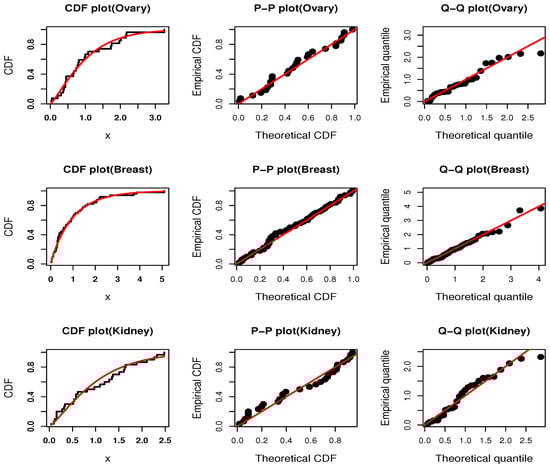
Figure 1. Empirical and theoretical CDF, P-P and Q-Q plots of Weibull distribution for survival times of cancer patients data.

Using observations of Table 2, the BAII-PHCS data are generated across three distinct categories, each representing different test facilities. More precisely, BAII-PHCS data are generated within different categories, incorporating different sample sizes $(n_1,n_2,n_3)=(27,50,30)$ and effective sample sizes $(m_1,m_2,m_3)=(23,37,25)$. Different censoring schemes are considered in each group, and the resulting BAII-PHCS observation for the survival times in cancer data are reported in Table 4.

Table 4. BAII-PHCS data for cancer data.

Data	T	Censoring	BAII-PHCS Data
Ovary	1.5	$(4,0^{\ast 22})$	0.3662, 0.3865, 0.4272, 0.4272, 0.4476, 0.4476, 0.6510, 0.6714, 0.7324,
			0.7731, 0.7935, 0.8138, 0.9766, 0.9969, 1.0783, 1.3835, 1.7294, 1.7498,
			1.9736, 2.0143, 2.1567, 2.1771, 3.2554
Breast	2	$(0^{\ast 18},13,0^{\ast 18})$	0.0203, 0.0406, 0.0406, 0.0609, 0.0812, 0.1218, 0.1218, 0.1421, 0.2030,
			0.2437, 0.2437, 0.2843, 0.2843, 0.3046, 0.3046, 0.3046, 0.3249, 0.3249,
			0.9748, 1.0154, 1.0560, 1.1169, 1.2388, 1.3200, 1.4012, 1.4419, 1.5434,
			1.6450, 1.9090, 2.0511, 2.0714, 2.1730, 2.2136, 2.6604, 3.7164, 3.8586,
			5.0974
Kidney	1.2	$(0^{\ast 24},5)$	0.0396, 0.0992, 0.1190, 0.1587, 0.1587, 0.1587, 0.2778, 0.3174, 0.3373,
			0.5158, 0.5357, 0.5753, 0.5753, 0.6150, 0.8134, 0.9722, 1.0912, 1.1904,
			1.2896, 1.3492, 1.3690, 1.5079, 1.6071, 1.6269, 1.6468,

For each category, by taking the differences in test facilities into account, we analyze BAII-PHCS cancer data using the Weibull model with parameters $\alpha$ and ${\beta }_i$, $i=1,2,3$. Different point estimates of parametric quantities are obtained. Further ACI intervals of parameters and reliability indices are obtained using MLE approach. The profile log-likelihood plot of $\alpha$ in Figure 2 exhibits an unimodal shape. We generate MCMC samples in order to evaluate corresponding Bayesian estimates. Figure 3 and Figure 4 represent convergence of MCMC samples using trace plots. Model parameters $(\alpha ,{\beta }_1,{\beta }_2,{\beta }_3,\beta )$ as well as reliability indices $S\left(0.5\right),H\left(0.5\right)$, and MTF, are estimated under MLE and Bayesian methods. The associated results are presented in Table 5.

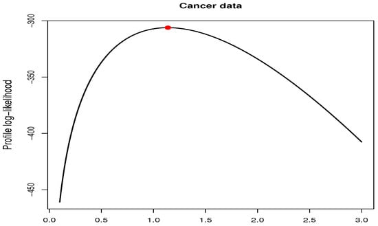
Figure 2. Profile log-likelihood plot for $\alpha$ under Cancer data.

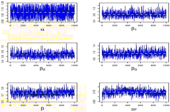
Figure 3. Trace plots of the model parameters and SF(0.5) for cancer patients data.

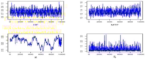
Figure 4. Trace plots of HF$\left(0.5\right)$, MTF, z and $\xi$ for cancer patients data.

Table 5. Point and interval estimates of parameter and reliability indices $(x_0=0.5)$ for cancer data.

	MLE				Bayes
		ACIs				HPD
Parameter	Estimates	Lower	Upper	Length	Estimates	Lower	Upper	Length
$\alpha$	1.139	0.922	1.356	0.434	1.052	1.006	1.120	0.114
${\beta }_1$	0.791	0.463	1.120	0.656	0.826	0.621	1.169	0.548
${\beta }_2$	0.630	0.413	0.847	0.434	0.666	0.447	0.871	0.424
${\beta }_3$	0.917	0.556	1.279	0.723	0.927	0.580	1.263	0.683
$\beta$	0.727	0.559	0.895	0.336	0.755	0.603	0.919	0.316
SF	0.719	0.666	0.771	0.105	0.695	0.640	0.729	0.079
HF	0.752	0.587	0.916	0.329	0.766	0.610	0.930	0.320
MDTF	1.263	1.023	1.504	0.482	1.295	1.130	1.549	0.419
z					0.243	0.093	0.371	0.279
$\xi$					0.436	0.013	1.370	1.357

6. Conclusions

In this paper, we introduced a novel block adaptive type-II progressive hybrid censoring scheme and derived useful inferences for reliability indices using the Weibull family of models. In addition to the likelihood-based approach for estimating model parameters, SF, HRF, MTF, and DDF function, we proposed a hierarchical Bayesian model to obtain the desired inferences. Furthermore, the existence and uniqueness of maximum likelihood estimators for the parameters were established. Monte Carlo simulations were applied to approximate complex posterior computations. Through extensive simulation studies and real-life applications, we observed that the proposed hierarchical Bayesian model, combined with Metropolis–Hastings sampling, provides an appealing alternative to traditional likelihood estimation methods. While this study focused on inference problems for the Weibull family, the results can be extended to other lifetime distributions, such as Kumaraswamy, Lomax, and inverse Weibull models. In addition, the Weibull-G family of distributions described by Bourguignon et al. [36] represents a mixture of the Weibull distribution with other continuous distributions, such as Weibull-uniform, Weibull-Weibull, Weibull-Lomax, and Weibull-Kumaraswamy. The specific distribution depends on the CDF of the associated distribution. Similarly, by employing parallel methodologies and generalization approaches, the derived results can also be extended to shape-scale families of distributions with a CDF of the form:

$$\begin{array}{c}\hfill F(x;\alpha ,\beta )=1-exp\left\{-\beta {\left(g\left(x\right)\right)}^{\alpha }\right\},\alpha ,\beta >0,x>0,\end{array}$$

where $g\left(x\right)$ is a differentiable and strictly increasing function of x such that $g\left(0^{+}\right)=0$ and $g\left(x\right)\to +\infty$ as $x\to +\infty$. Based on specific choices of ${\left(g\left(x\right)\right)}^{\alpha }$, well-known distributions such as Weibull extension, modified Weibull, Weibull, Pareto, Burr-type-XII, Lomax, and generalized Pareto distributions can be derived. A useful reference related to shape-scale family distributions is Maswadah [37].

Moreover, these results can be extended to other censoring schemes, such as type-II censoring, progressive first-failure censoring, and hybrid censoring. To further analyze the effect of differences across testing facilities in reliability engineering, it is also interesting to explore optimal design problems, which will be reported in future studies.

References

- Cohen, A.C. Progressively censored samples in life testing. Technometrics 1963, 5, 327–339. [Google Scholar] [CrossRef]
- Balakrishnan, N.; Sandhu, R.A. A simple simulational algorithm for generating progressive type-II censored samples. Am. Stat. 1995, 49, 229–230. [Google Scholar] [CrossRef]
- Balakrishnan, N.; Aggarwala, R. Progressive Censoring: Theory, Methods, and Applications; Birkhauser: Boston, MA, USA, 2000. [Google Scholar]
- Balakrishnan, N.; Cramer, E. The Art of Progressive Censoring: Applications to Reliability and Quality; Springer: New York, NY, USA, 2014. [Google Scholar]
- Wang, L. Inference of progressively censored competing risks data from Kumaraswamy distributions. J. Comput. Appl. Math. 2018, 343, 719–736. [Google Scholar] [CrossRef]
- Chandra, P.; Lodhi, C.; Tripathi, Y.M. Optimum plans for progressive censored competing risk data under Kies distribution. Sankhya B 2024, 86, 1–40. [Google Scholar] [CrossRef]
- Lodhi, C.; Tripathi, Y.M.; Bhattacharya, R. On a progressively censored competing risks data from Gompertz distribution. Commun. Stat.-Simul. Comput. 2023, 52, 1278–1299. [Google Scholar] [CrossRef]
- Singh, K.; Mahto, A.K.; Tripathi, Y.M.; Wang, L. Estimation in a multicomponent stress-strength model for progressive censored lognormal distribution. Proc. Inst. Mech. Eng. Part O J. Risk Reliab. 2024, 238, 622–642. [Google Scholar] [CrossRef]
- Singh, K.; Mahto, A.K.; Tripathi, Y.M.; Wang, L. Inference for reliability in a multicomponent stress–strength model for a unit inverse Weibull distribution under type-II censoring. Qual. Technol. Quant. Manag. 2024, 21, 147–176. [Google Scholar] [CrossRef]
- Mahto, A.K.; Tripathi, Y.M.; Kızılaslan, F. Estimation of reliability in a multicomponent stress-strength model for a general class of inverted exponentiated distributions under progressive censoring. J. Stat. Theory Pract. 2020, 14, 1–35. [Google Scholar] [CrossRef]
- Almetwally, E.M.; Jawa, T.M.; Sayed-Ahmed, N.; Park, C.; Zakarya, M.; Dey, S. Analysis of unit-Weibull based on progressive type-II censored with optimal scheme. Alex. Eng. J. 2023, 63, 321–338. [Google Scholar] [CrossRef]
- El-Sherpieny, E.S.A.; Almetwally, E.M.; Muhammed, H.Z. Bayesian and non-bayesian estimation for the parameter of bivariate generalized Rayleigh distribution based on clayton copula under progressive type-II censoring with random removal. Sankhya A 2023, 85, 1205–1242. [Google Scholar] [CrossRef]
- Maurya, R.K.; Tripathi, Y.M.; Sen, T.; Rastogi, M.K. On progressively censored inverted exponentiated Rayleigh distribution. J. Stat. Comput. Simul. 2019, 89, 492–518. [Google Scholar] [CrossRef]
- Lodhi, C.; Tripathi, Y.M.; Rastogi, M.K. Estimating the parameters of a truncated normal distribution under progressive type II censoring. Commun. Stat. Simul. Comput. 2021, 50, 2757–2781. [Google Scholar] [CrossRef]
- Kundu, D.; Joarder, A. Analysis of type-II progressively hybrid censored data. Comput. Stat. Data Anal. 2006, 50, 2509–2528. [Google Scholar] [CrossRef]
- Ng, H.K.T.; Kundu, D.; Chan, P.S. Statistical analysis of exponential lifetimes under an adaptive type-II progressive censoring scheme. Nav. Res. Logist. 2009, 56, 687–698. [Google Scholar] [CrossRef]
- Nassar, M.; Abo-Kasem, O.E. Estimation of the inverse Weibull parameters under adaptive type-II progressive hybrid censoring scheme. J. Comput. Appl. Math. 2017, 315, 228–239. [Google Scholar] [CrossRef]
- Dutta, S.; Dey, S.; Kayal, S. Bayesian survival analysis of logistic exponential distribution for adaptive progressive type-II censored data. Comput. Stat. 2024, 39, 2109–2155. [Google Scholar] [CrossRef]
- Elshahhat, A.; Dutta, S.; Abo-Kasem, O.E.; Mohammed, H.S. Statistical analysis of the Gompertz-Makeham model using adaptive progressively hybrid type-II censoring and its applications in various sciences. J. Radiat. Res. Appl. Sci. 2023, 16, 100644. [Google Scholar] [CrossRef]
- Gangopadhyay, A.K.; Mondal, R.; Lodhi, C.; Maiti, K. Bayesian inference on parameters and reliability characteristics for inverse Xgamma distribution under adaptive-general progressive type-II censoring. J. Radiat. Res. Appl. Sci. 2024, 17, 100890. [Google Scholar] [CrossRef]
- Nassar, M.; Abo-Kasem, O.; Zhang, C.; Dey, S. Analysis of Weibull distribution under adaptive type-II progressive hybrid censoring scheme. J. Indian Soc. Probab. Stat. 2018, 19, 25–65. [Google Scholar] [CrossRef]
- Ren, J.; Gui, W. Statistical analysis of adaptive type-II progressively censored competing risks for Weibull models. Appl. Math. Model. 2021, 98, 323–342. [Google Scholar] [CrossRef]
- Ren, J.; Gui, W. Inference and optimal censoring scheme for progressively type-II censored competing risks model for generalized Rayleigh distribution. Comput. Stat. 2021, 36, 479–513. [Google Scholar] [CrossRef]
- Almetwally, E.M.; Almongy, H.M.; ElSherpieny, E.A. Adaptive type-II progressive censoring schemes based on maximum product spacing with application of generalized Rayleigh distribution. J. Data Sci. 2019, 17, 802–831. [Google Scholar] [CrossRef]
- Almetwally, E.M.; Almongy, H.M.; Rastogi, M.K.; Ibrahim, M. Maximum product spacing estimation of Weibull distribution under adaptive type-II progressive censoring schemes. Ann. Data Sci. 2020, 7, 257–279. [Google Scholar] [CrossRef]
- Ahmadi, M.V.; Doostparast, M.; Ahmadi, J. Block censoring scheme with two-parameter exponential distribution. J. Stat. Comput. Simul. 2018, 88, 1229–1251. [Google Scholar] [CrossRef]
- Zhu, T. Reliability estimation for two-parameter Weibull distribution under block censoring. Reliab. Eng. Syst. Saf. 2020, 203, 107071. [Google Scholar] [CrossRef]
- Kumari, R.; Tripathi, Y.M.; Sinha, R.K.; Wang, L. Reliability estimation for bathtub-shaped distribution under block progressive censoring. Math. Comput. Simul. 2023, 213, 237–260. [Google Scholar] [CrossRef]
- Kumari, R.; Tripathi, Y.M.; Wang, L.; Sinha, R.K. Reliability estimation for Kumaraswamy distribution under block progressive type-II censoring. Statistics 2024, 58, 142–175. [Google Scholar] [CrossRef]
- Wang, L.; Wu, S.-J.; Lin, H.; Tripathi, Y.M. Inference for block progressive censored competing risks data from an inverted exponentiated exponential model. Qual. Reliab. Eng. Int. 2023, 39, 2736–2764. [Google Scholar] [CrossRef]
- Weibull, W. References on Weibull Distribution, FTL, A Report; Forsvarets Teletekniska Laboratorium: Stockholm, Sweden, 1977; FTL A-report A20:23. [Google Scholar]
- Murthy, D.P.; Xie, M.; Jiang, R. Weibull Models; Wiley: New York, NY, USA, 2004. [Google Scholar]
- Lai, C.D.; Murthy, D.N.P.; Xie, M. Weibull distributions. Wiley Interdiscip. Rev. Comput. Stat. 2011, 3, 282–287. [Google Scholar] [CrossRef]
- Cameron, E.; Pauling, L. Supplemental ascorbate in the supportive treatment of cancer: Reevaluation of prolongation of survival times in terminal human cancer. Proc. Natl. Acad. Sci. USA 1978, 75, 4538–4542. [Google Scholar] [CrossRef]
- Hand, D.J.; Daly, F.; McConway, K.; Lunn, D.; Ostrowski, E. A Handbook of Small Data Sets; CRC Press: London, UK, 1993. [Google Scholar]
- Bourguignon, M.; Silva, R.B.; Cordeiro, G.M. The Weibull-G family of probability distributions. J. Data Sci. 2014, 12, 53–68. [Google Scholar] [CrossRef]
- Maswadah, M. Improved maximum likelihood estimation of the shape-scale family based on the generalized progressive hybrid censoring scheme. J. Appl. Stat. 2022, 49, 2825–2844. [Google Scholar] [CrossRef] [PubMed]
Disclaimer/Publisher’s Note: The statements, opinions and data contained in all publications are solely those of the individual author(s) and contributor(s) and not of MDPI and/or the editor(s). MDPI and/or the editor(s) disclaim responsibility for any injury to people or property resulting from any ideas, methods, instructions or products referred to in the content. |
© 2024 by the authors. Licensee MDPI, Basel, Switzerland. This article is an open access article distributed under the terms and conditions of the Creative Commons Attribution (CC BY) license (https://creativecommons.org/licenses/by/4.0/).