Two-Player Nonzero-Sum Stochastic Differential Games with Switching Controls

Abstract

In this paper, a two-player nonzero-sum stochastic differential game problem is studied with both players using switching controls. A verification theorem associated with a set of variational inequalities is established as a sufficient criterion for Nash equilibrium, in which the equilibrium switching strategies for the two players, indicating when and where it is optimal to switch, are characterized in terms of the so-called switching regions and continuation regions. The verification theorem is proved in a piecewise way along the sequence of total decision times of the two players. Then, some detailed explanations are also provided to illustrate the idea why the conditions are imposed in the verification theorem.

1. Introduction

A differential game is concerned with the problem that multiple players make decisions, according to their own advantages and trade-off with other peers, in the context of dynamic systems. More precisely, suppose that there are N players acting on a dynamic system through their decisions $u_i$, and each of them has an individual cost functional $J_i(u_1,\dots ,u_N)$, $i=1,2,\dots ,N$. The goal is to find a Nash equilibrium $(u_1^{\ast },\dots ,u_N^{\ast })$ for the N players, which satisfies $J_i(u_1^{\ast },\dots ,u_N^{\ast })\le J_i(u_1^{\ast },\dots ,u_{i-1}^{\ast },u_i,u_{i+1}^{\ast },\dots ,u_N^{\ast })$, for $i=1,\dots ,N$, where $u_i$ is an arbitrary decision for Player i. The property of $(u_1^{\ast },\dots ,u_N^{\ast })$ means that when the N players act with $(u_1^{\ast },\dots ,u_N^{\ast })$, it is advantageous for them to maintain their decisions throughout. If one of them acts unilaterally to change a decision, it is penalized if the others maintain their initial decisions. The problem described above is called a nonzero-sum differential game. In this paper, we assume $N=2$ and focus our attention on the two-player case. In particular, if the dynamic system is given by a stochastic differential equation, then the game is called a nonzero-sum stochastic differential game, and there is much literature on this subject; see Hamadène et al. [1], Hamadène [2,3], Wu [4], and Sun and Yong [5]. On the other hand, recently, the theory of optimal control and differential game has been found to be very useful in the field of human–machine interaction systems; see [6,7,8].

Optimal switching is used to determine a sequence of stopping times at which to shift the mode of the control process to another. When there are more than two modes, it needs to decide not only when to switch, but also where to switch. As an important branch in control theory, optimal switching has been extensively investigated by means of variational inequalities (see Yong [9,10], Tang and Yong [11], Pham [12], and Song et al. [13]) or backward stochastic differential equations (see Hamadène and Jeanblanc [14], El Asri and Hamadène [15], Hamadène and Zhang [16], Hu and Tang [17], and El Asri [18,19]). In addition, the zero-sum switching game problems have been discussed by Tang and Hou [20], Hamadène et al. [21], and El Asri and Mazid [22]; it is noted that the nonzero-sum switching game problems have not ever been investigated. Apart from the mathematical interest in its own right, optimal switching enjoys a wide range of applications, such as resource extraction (Brekke and Øksendal [23]), investment decisions (Duckworth and Zervos [24]), and electricity production (Carmona and Ludkovski [25]).

In this paper, we consider, for the first time in the literature, a two-player nonzero-sum stochastic differential game with both players using switching controls. The main contribution of this paper is to establish a verification theorem (see Theorem 1) as a sufficient criterion for Nash equilibrium between the two players, in which a set of variational inequalities is given and a regularity condition is imposed to require, taking player 1 for example, the solution $V_1(x,i,j)$ to be $C^1$ on the opponent’s continuation region $D_{2,i,j}$, and to be $C^2$ on $D_{2,i,j}$ except for the boundary of its own continuation region $D_{1,i,j}$. It turns out that the Nash equilibrium strategies for the two players can be constructed based on these variational inequalities, and the solutions $V_1(x,i,j)$ and $V_2(x,i,j)$ coincide with the corresponding value functions (or, Nash equilibrium payoffs in the terminology of Buckdahn et al. [26]) of the two players.

On the one hand, it is emphasized that, if we just prove the verification theorem, then the regularity condition given is more strict than what we actually need; however, the seemingly superfluous regularity condition is really necessary if we want to further apply the the so-called smooth-fit principle to solve some specific examples, otherwise we cannot find enough pasting equations for the undetermined parameters. On the other hand, we would like to mention that in this paper, the verification theorem is proved in a piecewise or stage-by-stage way along the sequence of total decision times of the two players (here, a stage means a period between two adjacent decision times), which, to the best of our best knowledge, is new in the nonzero-sum switching game literature.

The rest of this paper is organized as follows. Section 2 formulates the nonzero-sum game problem under consideration. Section 3 states and proves the verification theorem. Finally, Section 4 concludes the paper with some further remarks.

2. Problem Formulation

Let R be the one-dimensional real space. For a subset $D\subset R$, $C\left(D\right)$, $C^1\left(D\right)$, and $C^2\left(D\right)$, denote the spaces of all real valued continuous, continuously differentiable, and twice continuously differentiable functions on D, respectively. Let $(\Omega ,\mathcal{F},P)$ be a probability space on which a one-dimensional standard Brownian motion $B\left(t\right)$, $t\ge 0$, is defined. ${\left\{{\mathcal{F}}_t\right\}}_{t\ge 0}$ denotes the natural filtration of $B(·)$ augmented by all the null sets.

Let the two players in the game be labeled Player 1 and Player 2. In order to formulate the problem precisely, we first provide the definition of admissible switching controls for the two players.

Definition 1.

Let ${\mathcal{N}}_1=\{1,\dots ,N_1\}$ and ${\mathcal{N}}_2=\{1,\dots ,N_2\}$ be two finite sets of possible modes for Player 1 and Player 2, respectively. An admissible switching control for Player 1 is a sequence of pairs ${({\tau }_m,{\xi }_m)}_{m\ge 1}$, where ${\left({\tau }_m\right)}_{m\ge 1}$ is a sequence of stopping times with ${\tau }_m<{\tau }_{m+1}$ and ${\tau }_m\to \infty$ as $m\to \infty$, representing the decisions on “when to switch," and ${\left({\xi }_m\right)}_{m\ge 1}$ is a sequence of ${\mathcal{N}}_1$-valued random variables with each ${\xi }_m$ being ${\mathcal{F}}_{{\tau }_m}$-measurable, representing the decisions on “where to switch." The collection of all admissible switching controls for Player 1 is denoted by ${\mathcal{U}}_1$.

An admissible switching control ${({\rho }_n,{\eta }_n)}_{n\ge 1}$ for Player 2 is defined similarly. The collection of all admissible switching controls for Player 2 is denoted as ${\mathcal{U}}_2$.

Remark 1.

Here, an example of electricity production management is provided to illustrate the meaning of “possible modes for players” in the Definition 1. Typically, a power plant has multiple modes, such as operating at full capacity, operating at partial capacity, or even shutting down all generators. Suppose that there are two managers running the power plant by switching the mode of the power plant from one to another, and the fixed costs are associated with these switchings. Both managers make decisions to maximize their payoffs and eventually reach a Nash equilibrium. In this example, the multiple modes of the power plant that can be chosen by the two managers are the so-called “possible modes for players”.

The state process $X\in R$ is described by the following:

$$\left\{\begin{array}{cc}\hfill dX\left(t\right)=& b\left(X\right(t\left)\right)dt+\sigma \left(X\right(t\left)\right)dB\left(t\right),t\ge 0,\hfill \\ \hfill X\left(0\right)=& x,\hfill \end{array}\right.$$

(1)

where $b,\sigma :R\mapsto R$ are two given functions satisfying the usual Lipschitz condition, so that (1) admits a unique strong solution. Note that the functions b and $\sigma$ and the functions f, ${\varphi }_1$, ${\varphi }_2$, ${\psi }_1$, ${\psi }_2$ appearing in the following payoff functionals are deterministic, as, in this paper, we adopt the verification theorem approach associated with a set of ordinary differential equations in the form of variational inequalities to deal with the game problem under consideration.

The payoff functionals for Player 1 and Player 2 to maximize are given, respectively, by

$$\begin{array}{cc}\hfill J_1(x,i,j;u_1,u_2)=& E[{\int }_0^{\infty }{e}^{-rt}{f}_1(X\left(t\right),u_1\left(t\right),u_2\left(t\right))dt\hfill \\ \hfill & -\sum _{m\ge 1}{e}^{-r{\tau }_m}{\varphi }_1({\xi }_{m-1},{\xi }_m)+\sum _{n\ge 1}{e}^{-r{\rho }_n}{\psi }_1({\eta }_{n-1},{\eta }_n)],\hfill \end{array}$$

and

$$\begin{array}{cc}\hfill J_2(x,i,j;u_1,u_2)=& E[{\int }_0^{\infty }{e}^{-rt}{f}_2(X\left(t\right),u_1\left(t\right),u_2\left(t\right))dt\hfill \\ \hfill & -\sum _{n\ge 1}{e}^{-r{\rho }_n}{\varphi }_2({\eta }_{n-1},{\eta }_n)+\sum _{m\ge 1}{e}^{-r{\tau }_m}{\psi }_2({\xi }_{m-1},{\xi }_m)],\hfill \end{array}$$

where $f:R\times {\mathcal{N}}_1\times {\mathcal{N}}_2\mapsto R$ is a given function, ${\varphi }_1:{\mathcal{N}}_1\times {\mathcal{N}}_1\mapsto R$ and ${\varphi }_2:{\mathcal{N}}_2\times {\mathcal{N}}_2\mapsto R$ are the switching costs for Player 1 and Player 2, respectively, ${\psi }_1:{\mathcal{N}}_1\times {\mathcal{N}}_1\mapsto R$ and ${\psi }_2:{\mathcal{N}}_2\times {\mathcal{N}}_2\mapsto R$ are the corresponding gains for Player 1 and Player 2 due to the opposites’ actions, respectively, and $\mu >0$ is the discount factor. It is emphasized that there are no specific conditions on the functions f, ${\varphi }_1$, ${\varphi }_2$, ${\psi }_1$, ${\psi }_2$; all of the conditions we need are listed in the verification theorem.

The objective is to find a Nash equilibrium $(u_1^{\ast },u_2^{\ast })\in {\mathcal{U}}_1\times {\mathcal{U}}_2$, i.e.,

$$\left\{\begin{array}{cc}\hfill J_1(x,i,j;u_1^{\ast },u_2^{\ast })\ge & J_1(x,i,j;u_1,u_2^{\ast }),\forall u_1\in {\mathcal{U}}_1,\hfill \\ \hfill J_2(x,i,j;u_1^{\ast },u_2^{\ast })\ge & J_2(x,i,j;u_1^{\ast },u_2),\forall u_2\in {\mathcal{U}}_2.\hfill \end{array}\right.$$

If such a Nash equilibrium exists, then we denote

$$\begin{array}{c}\hfill (V_1(x,i,j),V_2(x,i,j))=(J_1(x,i,j;u_1^{\ast },u_2^{\ast }),J_2(x,i,j;u_1^{\ast },u_2^{\ast }))\end{array}$$

as the corresponding value function. Note that $V_1,V_2$ are not uniquely defined, but depend on the Nash equilibrium under consideration.

Remark 2.

In this paper, we assume the Brownian motion and the state process to be one-dimensional just for simplicity of presentation. There is no essential difficulty to generalize the results to the multi-dimensional case, but with more complex notation.

3. Verification Theorem

In this section, we establish a verification theorem as a sufficient criterion that can be used to obtain a Nash equilibrium.

Let

$$\begin{array}{c}\hfill {\mathcal{M}}_1{V}_1(x,i,j)=\underset{k\ne i}{max}\{V_1(x,k,j)-{\varphi }_1(i,k)\},\end{array}$$

and

$$\begin{array}{c}\hfill {\mathcal{M}}_2{V}_2(x,i,j)=\underset{l\ne j}{max}\{V_2(x,i,l)-{\varphi }_2(j,l)\}.\end{array}$$

Then, let

$$\begin{array}{c}\hfill {\mathcal{N}}_1{V}_1(x,i,j)=V_1(x,i,l)+{\psi }_1(j,l),\end{array}$$

and

$$\begin{array}{c}\hfill {\mathcal{N}}_2{V}_2(x,i,j)=V_2(x,k,j)+{\psi }_2(i,k).\end{array}$$

Remark 3.

The definitions of ${\mathcal{M}}_1{V}_1(x,i,j)$ and ${\mathcal{M}}_2{V}_2(x,i,j)$ have an immediate explanation: If Player 1 (respectively, Player 2) makes a switching from i to k (respectively, j to l), then the present Nash equilibrium payoff can be written as $V_1(x,k,j)-{\varphi }_1(i,k)$ (respectively, $V_2(x,i,l)-{\varphi }_2(j,l)$); we have considered the payoff in the present mode of the switching control and the switching cost. The maximum point of ${\mathcal{M}}_1{V}_1(x,i,j)$ (respectively, ${\mathcal{M}}_2{V}_2(x,i,j)$) is actually the best new mode that Player 1 (respectively, Player 2) would choose in case it wants to switch; otherwise, it would be in its interest to deviate by the definition of the Nash equilibrium.

Similarly, ${\mathcal{N}}_1{V}_1(x,i,j)$ (respectively, ${\mathcal{N}}_2{V}_2(x,i,j)$) represents the payoff for Player 1 (respectively, Player 2) when Player 2 (respectively, Player 1) takes the best switching action and behaves optimally afterward.

Let

$$\begin{array}{c}\hfill D_{1,i,j}=\{V_1(x,i,j)-{\mathcal{M}}_1{V}_1(x,i,j)>0\},\end{array}$$

and

$$\begin{array}{c}\hfill D_{2,i,j}=\{V_2(x,i,j)-{\mathcal{M}}_2{V}_2(x,i,j)>0\}.\end{array}$$

In fact, $D_{1,i,j}$ (respectively, $D_{2,i,j}$) is the so-called continuation (or, no-switching) region for Player 1 (respectively, Player 2), in which it is better for Player 1 (respectively, Player 2) to do nothing than make a switching; see Figure 1 for a graphical representation of $D_{1,i,j}$ and $D_{2,i,j}$. The boundaries of $D_{1,i,j}$ and $D_{2,i,j}$ are denoted by $\partial D_{1,i,j}$ and $\partial D_{2,i,j}$, respectively.

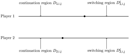
Figure 1. A graphical representation of $D_{1,i,j}$ and $D_{2,i,j}$.

Denote

$$\begin{array}{c}\hfill \mathcal{L}\phi \left(x\right)=b\left(x\right){\phi }^{\prime }\left(x\right)+{\displaystyle \frac{1}{2}}{\sigma }^2\left(x\right){\phi }^{″}\left(x\right),\end{array}$$

where ${\phi }^{\prime }\left(x\right)$ and ${\phi }^{″}\left(x\right)$ are the first-order and second-order derivatives of an arbitrary twice differentiable function $\phi$, respectively.

Now, we state and prove the verification theorem for the nonzero-sum stochastic differential game with switching controls.

Theorem 1.

Let $V_1$ and $V_2$ be real-valued functions, such that:

(i) For $i,j\in S$,

$$\begin{array}{c}\hfill V_1(·,i,j)\in C^2(D_{2,i,j}\backslash ({\cup }_{i\in {\mathcal{N}}_1,j\in {\mathcal{N}}_2}\partial D_{1,i,j}))\cap C^1\left(D_{2,i,j}\right)\cap C\left(R\right),\end{array}$$

and

$$\begin{array}{c}\hfill V_2(·,i,j)\in C^2(D_{1,i,j}\backslash ({\cup }_{i\in {\mathcal{N}}_1,j\in {\mathcal{N}}_2}\partial D_{2,i,j}))\cap C^1\left(D_{1,i,j}\right)\cap C\left(R\right).\end{array}$$

(ii) For $i,j\in S$ and $x\in R$,

$$\begin{array}{c}\hfill V_1(x,i,j)-{\mathcal{M}}_1{V}_1(x,i,j)\ge 0,\end{array}$$

and

$$\begin{array}{c}\hfill V_2(x,i,j)-{\mathcal{M}}_2{V}_2(x,i,j)\ge 0.\end{array}$$

(iii) For $i,j\in S$ and $x\in D_{2,i,j}$,

$$min\left\{r{V}_1(x,i,j)-\mathcal{L}{V}_1(x,i,j)-f_1(x,i,j),V_1(x,i,j)-{\mathcal{M}}_1{V}_1(x,i,j)\right\}=0.$$

(2)

(iv) For $i,j\in S$ and $x\in D_{1,i,j}$,

$$min\left\{r{V}_2(x,i,j)-\mathcal{L}{V}_2(x,i,j)-f_2(x,i,j),V_2(x,i,j)-{\mathcal{M}}_2{V}_2(x,i,j)\right\}=0.$$

(3)

(v) For $i,j\in S$ and $x\in D_{2,i,j}^c=\{V_2(x,i,j)-{\mathcal{M}}_2{V}_2(x,i,j)=0\}$,

$$\begin{array}{c}\hfill V_1(x,i,j)-{\mathcal{N}}_1{V}_1(x,i,j)=0.\end{array}$$

(4)

(vi) For $i,j\in S$ and $x\in D_{1,i,j}^c=\{V_1(x,i,j)-{\mathcal{M}}_1{V}_1(x,i,j)=0\}$,

$$\begin{array}{c}\hfill V_2(x,i,j)-{\mathcal{N}}_2{V}_2(x,i,j)=0.\end{array}$$

(5)

Define $u_1^{\ast }={({\tau }_m^{\ast },{\xi }_m^{\ast })}_{m\ge 1}$ and $u_2^{\ast }={({\rho }_n^{\ast },{\eta }_n^{\ast })}_{n\ge 1}$ inductively as

$$\left\{\begin{array}{cc}\hfill {\tau }_m^{\ast }=& \underset{t>{\tau }_{m-1}^{\ast }}{inf}\{X^{u_1^{\ast },u_2^{\ast }}\left(t\right)\notin D_{1,u_1^{\ast }\left(t\right),u_2^{\ast }\left(t\right)}\},\hfill \\ \hfill {\xi }_m^{\ast }=& arg\underset{k\ne {\xi }_{m-1}^{\ast }}{max}\{V_1(X^{u_1^{\ast },u_2^{\ast }}\left({\tau }_m^{\ast }\right),k,u_2^{\ast }\left({\tau }_m^{\ast }\right))-{\varphi }_1({\xi }_{m-1}^{\ast },k)\},\hfill \end{array}\right.$$

(6)

and

$$\left\{\begin{array}{cc}\hfill {\rho }_n^{\ast }=& \underset{t>{\rho }_{n-1}^{\ast }}{inf}\{X^{u_1^{\ast },u_2^{\ast }}\left(t\right)\notin D_{2,u_1^{\ast }\left(t\right),u_2^{\ast }\left(t\right)}\},\hfill \\ \hfill {\eta }_n^{\ast }=& arg\underset{l\ne {\eta }_{n-1}^{\ast }}{max}\{V_2(X^{u_1^{\ast },u_2^{\ast }}\left({\rho }_n^{\ast }\right),u_1^{\ast }\left({\rho }_n^{\ast }\right),l)-{\varphi }_2({\eta }_{n-1}^{\ast },l)\}.\hfill \end{array}\right.$$

(7)

Then, we have that $(u_1^{\ast },u_2^{\ast })$ is a Nash equilibrium for the two players and $V_1,V_2$ are the corresponding value functions of the game.

Remark 4.

It should be noticed that along the boundaries of $D_{1,i,j}$ (respectively, $D_{2,i,j}$), the function $V_1(x,i,j)$ (respectively, $V_2(x,i,j)$), $i\in \mathcal{M}$, only belongs to $C^1$, but does not necessarily belong to $C^2$ on $D_{2,i,j}$ (respectively, $D_{1,i,j}$). In this situation, we can apply the smooth approximation argument introduced by Øksendal [27] (Theorem 10.4.1 and Appendix D) to complement the smoothness needed for Itô’s formula. Here, in this proof, for convenience, we simply consider $V_1(x,i,j)$ (respectively, $V_2(x,i,j)$), $i\in \mathcal{M}$, to be $C^2$ on $D_{2,i,j}$ (respectively, $D_{1,i,j}$); in this connection, see also Guo and Zhang [28] (Theorem 3.1) and [29] (Theorem 2) and Aïd et al. [30] (Theorem 1).

Proof. 

We only show the part for Player 1, and the counterpart for Player 2 is symmetric. We first prove that

$$\begin{array}{c}\hfill V_1(x,i,j)\ge J_1(x,i,j;u_1,u_2^{\ast }),\end{array}$$

where $u_1$ is an arbitrary switching control for Player 1. Denote ${\left({\nu }_k\right)}_{k\ge 1}$ (with ${\nu }_0=0$) as the sequence of total switching times in the game: at each ${\nu }_k$, we have either ${\nu }_k={\tau }_m$ for some m or ${\nu }_k={\rho }_n^{\ast }$ for some n. Then, based on ${\left({\nu }_k\right)}_{k\ge 1}$, the payoff functional for Player 1 can be rewritten as

$$\begin{array}{cc}\hfill J_1(x,i,j;u_1,u_2^{\ast })=& E[{\int }_0^{\infty }{e}^{-rt}{f}_1(X^{u_1,u_2^{\ast }}\left(t\right),u_1\left(t\right),u_2^{\ast }\left(t\right))dt\hfill \\ \hfill & +\sum _{k\ge 1}{e}^{-r{\nu }_k}\left\{-{\varphi }_1({\xi }_{m-1},{\xi }_m)1_{\{{\nu }_k={\tau }_m\}}+{\psi }_1({\eta }_{n-1}^{\ast },{\eta }_n^{\ast })1_{\{{\nu }_k={\rho }_n^{\ast }\}}\right\}].\hfill \end{array}$$

(8)

Applying Itô’s formula to $e^{-rt}{V}_1(X^{u_1,u_2^{\ast }}\left(t\right),u_1\left({\nu }_{k-1}\right),u_2^{\ast }\left({\nu }_{k-1}\right))$ between ${\nu }_{k-1}$ and ${\nu }_k$, $k\ge 1$, we have

$$\begin{array}{cc}\hfill & E[e^{-r{\nu }_k}{V}_1(X^{u_1,u_2^{\ast }}\left({\nu }_k\right),u_1\left({\nu }_{k-1}\right),u_2^{\ast }\left({\nu }_{k-1}\right))\hfill \\ \hfill & -e^{-r{\nu }_{k-1}}{V}_1(X^{u_1,u_2^{\ast }}\left({\nu }_{k-1}\right),u_1\left({\nu }_{k-1}\right),u_2^{\ast }\left({\nu }_{k-1}\right))]\hfill \\ \hfill =& E\left[{\int }_{{\nu }_{k-1}}^{{\nu }_k}{e}^{-rt}\left\{-(r-\mathcal{L})V_1(X^{u_1,u_2^{\ast }}\left(t\right),u_1\left({\nu }_{k-1}\right),u_2^{\ast }\left({\nu }_{k-1}\right))\right\}dt\right]\hfill \\ \hfill \le & -E\left[{\int }_{{\nu }_{k-1}}^{{\nu }_k}{e}^{-rt}{f}_1(X^{u_1,u_2^{\ast }}\left(t\right),u_1\left({\nu }_{k-1}\right),u_2^{\ast }\left({\nu }_{k-1}\right))dt\right]\hfill \\ \hfill =& -E\left[{\int }_{{\nu }_{k-1}}^{{\nu }_k}{e}^{-rt}{f}_1(X^{u_1,u_2^{\ast }}\left(t\right),u_1\left(t\right),u_2^{\ast }\left(t\right))dt\right],\hfill \end{array}$$

where the inequality follows from condition (iii), as $X^{u_1,u_2^{\ast }}\left(t\right)\in D_{2,u_1\left(t\right),u_2^{\ast }\left(t\right)}$ when $t\in ({\nu }_{k-1},{\nu }_k)$ and the last equality is due to the fact that no switching occurs between ${\nu }_{k-1}$ and ${\nu }_k$, thus, we have $u_1\left(t\right)\equiv u_1\left({\nu }_{k-1}\right)$ and $u_2\left(t\right)\equiv u_2^{\ast }\left({\nu }_{k-1}\right)$.

Summing the indices $k\ge 1$, we have

$$\begin{array}{cc}\hfill & \sum _{k\ge 1}E\left[e^{-r{\nu }_k}\{V_1(X^{u_1,u_2^{\ast }}\left({\nu }_k\right),u_1\left({\nu }_{k-1}\right),u_2^{\ast }\left({\nu }_{k-1}\right))-V_1(X^{u_1,u_2^{\ast }}\left({\nu }_k\right),u_1\left({\nu }_k\right),u_2^{\ast }\left({\nu }_k\right))\}\right]\hfill \\ \hfill \le & V_1(x,i,j)-E\left[{\int }_0^{\infty }{e}^{-rt}{f}_1(X^{u_1,u_2^{\ast }}\left(t\right),u_1\left(t\right),u_2^{\ast }\left(t\right))dt\right].\hfill \end{array}$$

(9)

Combining (8) and (9) yields

$$\begin{array}{cc}\hfill J_1(x,i,j;u_1,u_2^{\ast })\le V_1(x,i,j)& +\sum _{k\ge 1}{e}^{-r{\nu }_k}\left\{V_1\right(X^{u_1,u_2^{\ast }}\left({\nu }_k\right),u_1\left({\nu }_k\right),u_2^{\ast }\left({\nu }_k\right))\hfill \\ \hfill & -V_1(X^{u_1,u_2^{\ast }}\left({\nu }_k\right),u_1\left({\nu }_{k-1}\right),u_2^{\ast }\left({\nu }_{k-1}\right))\hfill \\ \hfill & -{\varphi }_1({\xi }_{m-1},{\xi }_m)1_{\{{\nu }_k={\tau }_m\}}+{\psi }_1({\eta }_{n-1}^{\ast },{\eta }_n^{\ast })1_{\{{\nu }_k={\rho }_n^{\ast }\}}\}.\hfill \end{array}$$

(10)

In the following, the analysis is divided into three cases:

(a) If ${\nu }_r={\tau }_m$ for some m, then

$$\begin{array}{cc}\hfill & V_1(X^{u_1,u_2^{\ast }}\left({\nu }_k\right),u_1\left({\nu }_{k-1}\right),u_2^{\ast }\left({\nu }_{k-1}\right))\hfill \\ \hfill =& V_1(X^{u_1,u_2^{\ast }}\left({\nu }_k\right),u_1\left({\nu }_{k-1}\right),u_2^{\ast }\left({\nu }_k\right))\hfill \\ \hfill \ge & V_1(X^{u_1,u_2^{\ast }}\left({\nu }_k\right),u_1\left({\nu }_k\right),u_2^{\ast }\left({\nu }_k\right))-{\varphi }_1({\xi }_{m-1},{\xi }_m).\hfill \end{array}$$

(11)

(b) If ${\nu }_r={\rho }_n^{\ast }$ for some n, then

$$\begin{array}{cc}\hfill & V_1(X^{u_1,u_2^{\ast }}\left({\nu }_k\right),u_1\left({\nu }_{k-1}\right),u_2^{\ast }\left({\nu }_{k-1}\right))\hfill \\ \hfill =& V_1(X^{u_1,u_2^{\ast }}\left({\nu }_k\right),u_1\left({\nu }_k\right),u_2^{\ast }\left({\nu }_{k-1}\right))\hfill \\ \hfill =& V_1(X^{u_1,u_2^{\ast }}\left({\nu }_k\right),u_1\left({\nu }_k\right),u_2^{\ast }\left({\nu }_k\right))+{\psi }_1({\eta }_{n-1}^{\ast },{\eta }_n^{\ast }).\hfill \end{array}$$

(12)

(c) If ${\nu }_r={\tau }_m={\rho }_n^{\ast }$ simultaneously for some m and n, then

$$\begin{array}{cc}\hfill & V_1(X^{u_1,u_2^{\ast }}\left({\nu }_k\right),u_1\left({\nu }_{k-1}\right),u_2^{\ast }\left({\nu }_{k-1}\right))\hfill \\ \hfill =& V_1(X^{u_1,u_2^{\ast }}\left({\nu }_k\right),u_1\left({\nu }_{k-1}\right),u_2^{\ast }\left({\nu }_{k-1}\right))-V_1(X^{u_1,u_2^{\ast }}\left({\nu }_k\right),u_1\left({\nu }_k\right),u_2^{\ast }\left({\nu }_{k-1}\right))\hfill \\ \hfill & +V_1(X^{u_1,u_2^{\ast }}\left({\nu }_k\right),u_1\left({\nu }_k\right),u_2^{\ast }\left({\nu }_{k-1}\right))-V_1(X^{u_1,u_2^{\ast }}\left({\nu }_k\right),u_1\left({\nu }_k\right),u_2^{\ast }\left({\nu }_k\right))\hfill \\ \hfill & +V_1(X^{u_1,u_2^{\ast }}\left({\nu }_k\right),u_1\left({\nu }_k\right),u_2^{\ast }\left({\nu }_k\right))\hfill \\ \hfill \le & V_1(X^{u_1,u_2^{\ast }}\left({\nu }_k\right),u_1\left({\nu }_k\right),u_2^{\ast }\left({\nu }_k\right))-{\varphi }_1({\xi }_{m-1},{\xi }_m)+{\psi }_1({\eta }_{n-1}^{\ast },{\eta }_n^{\ast }).\hfill \end{array}$$

(13)

From (10)–(13), we have

$$\begin{array}{c}\hfill V_1(x,i,j)\ge J_1(x,i,j;u_1,u_2^{\ast }).\end{array}$$

On the other hand, the proof of

$$\begin{array}{c}\hfill V_1(x,i,j)=J_1(x,i,j;u_1^{\ast },u_2^{\ast })\end{array}$$

is the same as above, but with all inequalities becoming equalities. □

Remark 5.

Here, we provide some comments on the conditions (i)–(vi) given in the verification theorem. First, the condition (i) is the regularity requirement on the solutions of the variational inequalities. It is important for us, in specific cases, to solve the variational inequalities and obtain some analytical solutions by using the so-called smooth-fit principle. The condition (ii) is a typical assumption in optimal switching control theory, which comes from the dynamic programming principle. Regarding the condition (iii), if Player 2 does not make a switching (i.e., $V_2(x,i,j)-{\mathcal{M}}_2{V}_2(x,i,j)>0$), then the problem for Player 1 becomes a classical one-player optimal switching control problem, so we have (2). On the contrary, if Player 2 makes a switching (i.e., $V_2(x,i,j)-{\mathcal{M}}_2{V}_2(x,i,j)=0$), by the definition of Nash equilibrium, we expect that Player 1 does not lose anything. This is equivalent to (4) in condition (v); otherwise, it would be in its interest to deviate. Finally, the conditions (iv) and (vi) on $V_2(x,i,j)$ are imposed for the same reason.

Remark 6.

The proof for the case with three or more than three players can be given in a similar way to that of Theorem 1. Note that in the proof of Theorem 1, we show the property of the Nash equilibrium, that $V_1(x,i,j)=J_1(x,i,j;u_1^{\ast },u_2^{\ast })$ and $V_2(x,i,j)=J_2(x,i,j;u_1^{\ast },u_2^{\ast })$ separately and independently. It can be naturally generalized to the case with three or more than three players, and one needs only to modify accordingly the conditions (i)–(vi) imposed on $V_1$ and $V_2$ to $V_p$ for $p\ge 3$ in Theorem 1.

4. Concluding Remarks

This paper is the first attempt to study a two-player nonzero-sum stochastic differential game with both players using switching controls. The verification theorem method is adopted with a set of variational inequalities and an appropriate regularity condition is proposed for Nash equilibriums.

It is mentioned that this paper is mainly devoted to the theoretical aspect of a stochastic differential game with switching controls. On the other hand, the numerical aspect is also an important and interesting issue, and it is very useful to apply the verification theorem for solving some practical problems arising from real world. We will consider this topic in our future study.

References

- Hamadène, S.; Lepeltier, J.P.; Peng, S. BSDEs with continuous coefficients and stochastic differential games. In Backward Stochastic Differential Equations (Paris, 1995–1996); Pitman Research Notes in Mathematics Series 364; Longman: Harlow, UK, 1997; pp. 115–128. [Google Scholar]
- Hamadène, S. Backward-forward SDE’s and stochastic differential games. Stoch. Process. Appl. 1998, 77, 1–15. [Google Scholar] [CrossRef]
- Hamadène, S. Nonzero sum linear-quadratic stochastic differential games and backward-forward equations. Stoch. Anal. Appl. 1999, 17, 117–130. [Google Scholar] [CrossRef]
- Wu, Z. Forward-backward stochastic differential equations, linear quadratic stochastic optimal control and nonzero sum differential games. J. Syst. Sci. Complex. 2005, 18, 179–192. [Google Scholar]
- Sun, J.; Yong, J. Linear-quadratic stochastic two-person nonzero-sum differential games: Open-loop and closed-loop Nash equilibria. Stoch. Process. Appl. 2019, 129, 381–418. [Google Scholar] [CrossRef]
- Kille, S.; Leibold, P.; Karg, P.; Varga, B.; Hohmann, S. Human-variability-respecting optimal control for physical human-machine interaction. arXiv 2024, arXiv:2405.03502. [Google Scholar]
- Kille, S.; Varga, B.; Hohmann, S. Study on human-variability-respecting optimal control affecting human interaction experience. arXiv 2024, arXiv:2408.08620. [Google Scholar]
- Varga, B. Toward adaptive cooperation: Model-based shared control using LQ-differential games. arXiv 2024, arXiv:2403.11146. [Google Scholar] [CrossRef]
- Yong, J. Differential games with switching strategies. J. Math. Anal. Appl. 1990, 145, 455–469. [Google Scholar] [CrossRef]
- Yong, J. A zero-sum differential game in a finite duration with switching strategies. SIAM J. Control Optim. 1990, 28, 1234–1250. [Google Scholar] [CrossRef]
- Tang, S.; Yong, J. Finite horizon stochastic optimal switching and impulse controls with a viscosity solution approach. Stochastics 1993, 45, 145–176. [Google Scholar] [CrossRef]
- Pham, H. On the smooth-fit property for one-dimensional optimal switching problem. In Séminaire de Probabilités XL; Springer: Berlin/Heidelberg, Germany, 2007; pp. 187–199. [Google Scholar]
- Song, Q.; Yin, G.; Zhu, C. Optimal switching with constraints and utility maximization of an indivisible market. SIAM J. Control Optim. 2012, 50, 629–651. [Google Scholar] [CrossRef]
- Hamadène, S.; Jeanblanc, M. On the statring and stopping problem: Applications in reversible investments. Math. Oper. Res. 2007, 32, 182–192. [Google Scholar] [CrossRef]
- Asri, B.E.; Hamadène, S. The finite horizon optimal multi-modes switching problem: The viscosity solution approach. Appl. Math. Optim. 2009, 60, 213–235. [Google Scholar] [CrossRef]
- Hamadène, S.; Zhang, J. Switching problem and related system of reflected backward SDEs. Stoch. Process. Appl. 2010, 120, 403–426. [Google Scholar] [CrossRef]
- Hu, Y.; Tang, S. Multi-dimensional BSDE with oblique reflection and optimal switching. Probab. Theory Relat. Fields 2010, 147, 89–121. [Google Scholar] [CrossRef]
- Asri, B.E. Optimal multi-modes switching problem in infinite horizon. Stoch. Dyn. 2010, 10, 231–261. [Google Scholar] [CrossRef]
- Asri, B.E. Stochastic optimal multi-modes switching with a viscosity solution approach. Stoch. Process. Appl. 2013, 123, 579–602. [Google Scholar] [CrossRef][Green Version]
- Tang, S.; Hou, S.H. Switching games of stochastic differential systems. SIAM J. Control Optim. 2007, 46, 900–929. [Google Scholar] [CrossRef]
- Hamadène, S.; Martyr, R.; Moriarty, J. A probabilistic verification theorem for the finite horizon two-player zero-sum optimal switching game in continuous time. Adv. Appl. Probab. 2019, 51, 425–442. [Google Scholar] [CrossRef]
- Asri, B.E.; Mazid, S. Stochastic differential switching game in infinite horizon. J. Math. Anal. Appl. 2019, 474, 793–813. [Google Scholar] [CrossRef]
- Brekke, K.A.; Øksendal, B. Optimal switching in an economic activity under uncertainty. SIAM J. Control Optim. 1994, 32, 1021–1036. [Google Scholar] [CrossRef]
- Duckworth, K.; Zervos, M. A model for investment decisions with switching costs. Ann. Appl. Probab. 2001, 11, 239–260. [Google Scholar] [CrossRef]
- Carmona, R.; Ludkovski, M. Pricing asset scheduling flexibility using optimal switching. Appl. Math. Financ. 2008, 15, 405–447. [Google Scholar] [CrossRef]
- Buckdahn, R.; Cardaliaguet, P.; Rainer, C. Nash equilibrium payoffs for nonzero-sum stochastic differential games. SIAM J. Control Optim. 2004, 43, 624–642. [Google Scholar] [CrossRef]
- Øksendal, B. Stochastic Differential Equations, 6th ed.; Springer: Berlin/Heidelberg, Germany, 2003. [Google Scholar]
- Guo, X.; Zhang, Q. Closed-form solutions for perpetual American put options with regime switching. SIAM J. Appl. Math. 2004, 64, 2034–2049. [Google Scholar]
- Guo, X.; Zhang, Q. Optimal selling rules in a regime switching market. IEEE Trans. Automat. Control 2005, 50, 1450–1455. [Google Scholar] [CrossRef]
- Aïd, R.; Basei, M.; Callegaro, G.; Campi, L.; Vargiolu, T. Nonzero-sum stochastic differential games with impulse controls: A verification theorem with applications. Math. Oper. Res. 2020, 45, 205–232. [Google Scholar] [CrossRef]
Disclaimer/Publisher’s Note: The statements, opinions and data contained in all publications are solely those of the individual author(s) and contributor(s) and not of MDPI and/or the editor(s). MDPI and/or the editor(s) disclaim responsibility for any injury to people or property resulting from any ideas, methods, instructions or products referred to in the content. |
© 2024 by the authors. Licensee MDPI, Basel, Switzerland. This article is an open access article distributed under the terms and conditions of the Creative Commons Attribution (CC BY) license (https://creativecommons.org/licenses/by/4.0/).