Abstract
In this paper, two systematic control design strategies are proposed for strict-feedback nonholonomic systems with full-state constraints to solve stabilization and adaptive stabilization problems. The stabilization schemes involve the introduction of state scaling, the barrier Lyapunov function (BLF), the integrator backstepping method, and the tuning function approach. In addition, a discontinuous switching control strategy is proposed to achieve the control goal if the first system state’s initial state is confined to zero. In both stabilization and adaptive stabilization control, the system states can be regulated at the origin, and meanwhile, the full-state constraints are realized. Finally, it is shown that the simulation results are consistent with the theory analysis results, which further demonstrates the effectiveness of the proposed control schemes.
Keywords:
nonholonomic control systems; stabilization; adaptive stabilization; full-state constraints; barrier Lyapunov function MSC:
93D15; 93D21
1. Introduction
Generally, a nonintegrable speed constraint can be formulated for a motion system running on a smooth horizontal plane since there is no sideslip. Nonholonomic systems refer to these motion systems which suffer from nonintegrable speed or acceleration constraints [1], such as rear-driven mobile robots and knife edge motion [2]. Various nonholonomic systems arise from practical engineering applications, especially with the high complexity of robot systems, the large number of applications of unmanned aerial vehicles, unmanned vehicles, and the wide adoption of large, flexible intelligent manufacturing systems.
In the literature, Brockett’s second example is described as
Although the originally proposed nonholonomic systems are seemingly driftless nonlinear systems, both their stabilization and tracking control problems have brought about many tough and thorny issues that cannot be directly solved by the traditional nonlinear control approaches. Brockett pointed out in [3] that there were no smooth, even continuous time-invariant stabilizing controllers for nonholonomic systems, although these systems could be formed into chained forms [1]. Therefore, discontinuous time-invariant, smooth time-varying, and hybrid control methods have become the most effective weapons to address the related stabilization control designs [4,5,6] even for stochastic nonholonomic systems [7,8].
Tracking control is mainly investigated for driftless nonholonomic systems including multiple-system cases, while stabilization is commonly addressed for uncertain nonholonomic systems. The control problems associated with stabilization further involve fast control containing finite-time or fixed-time control [9,10], input-saturated control [11], anti-disturbance control [12], and model predictive control [13]. In recent years, safe control, which can be classified into information security and physical security, has grasped extensive attention in control community. State-constrained control belongs to physical security and has been widely studied for nonlinear systems. When reviewing the existing results, it can be claimed that the BLF-based methods are the most commonly utilized tools to address state-constrained problems of nonlinear systems, such as those in [14,15,16,17,18]. The rapid development of control technologies facilitates the combination of state-constrained control and other control problems, such as neural network control [19], fuzzy control [20], finite-time control [21], and anti-disturbance control [22]. It should be mentioned that the fully actuated system approach has also been applied to solve the stabilization issues associated with nonholonomic systems in recent years, such as in [23,24,25,26].
In the literature, some works have been reported on nonholonomic systems with full-state or output-state constraints. The authors of [27] studied the tracking controller design for an uncertain nonholonomic system under time-varying disturbances and full-state constraints. The authors of [28] proposed the the fixed-time trajectory-tracking switching control for a full-state constrained nonholonomic system. The authors of [29,30] focused on the tracking controllers for two classes of state-constrained nonholonomic systems. The authors of [31] investigated the adaptive neural control for stochastic nonholonomic systems suffered from unknown covariance noise and full-state constraints. The authors of [32] elaborated upon the MPC-based cooperative controller design for nonholonomic system mobile agents with constraints and disturbances. The authors of [33] provided an anti-disturbance stabilization controller for a class of full-state constrained nonholonomic systems. The authors of [34] studied the fixed-time stabilization issue for uncertain nonholonomic systems under time-varying state constraints. The authors of [35] considered the cooperative tracking controller of multiple state-constrained nonholonomic wheeled mobile robots. The existing works studied either the output-state constrained problem or full-state constrained problem with bounded stability. This in turn implies that it is meaningful to address a full-state constrained controller with asymptotical convergence for nonholonomic systems. However, to achieve this control intention, the encountered difficulty focuses on how to construct a new non-constant input to drive the system state and maintain the desired state constraint in the second control stage.
This work studies both the stabilization and adaptive stabilization control problems of nonholonomic systems in strict feedback form subjected to full-state constraints. The summarized main contributions of this submitted work are as follows:
- (1)
- The state-constrained stabilization control issue is addressed roundly for a strict feedback nonholonomic system with drift nonlinearities and parameter uncertainties by imposing the linear growth restriction on the drift nonlinearities.
- (2)
- The constraint adaptive stabilization controller is also developed with no restrictions on the drift nonlinearities. It is shown that both the robust and adaptive stabilization controllers can simultaneously accomplish the asymptotic regulation and full-state constraint tasks.
- (3)
- When , nonzero constant action is the most commonly used method to drive the state away from zero [8,36]. Different from this, in this paper, we provide a new non-constant discontinuous switching approach to realize simultaneously both the stabilization control aims and the desired state constraints.
2. Robust Stabilization of Uncertain Nonholonomic Systems
In this section, we consider the following complicated version of uncertain nonholonomic systems:
where represents the system state vector, ’s stands for the uncertain nonlinear functions, including the neglected dynamics and the possible modeling errors, ’s represents the disturbed virtual control directions, and and are control inputs. In the sequel, for the state , . For , we first assume that is uniformly Lipschitz in .
Now, the control attention focuses on designing robust stabilization control laws such that the system in Equation (1) is asymptotically stable, while the full-state constraints are not violated, where represents positive constants. In order to accomplish this control objective, the following assumptions are orderly and are given as
Assumption 1.
For each virtual control direction , we assume that two positive known constants and can be found in such a way that
Assumption 2.
For uncertain functions , suppose that there are known nonnegative functions such that
Remark 1.
Assumption 1 has been commonly used in the stabilization control of nonholonomic systems, such as in [4,7,10].
Two frequently used lemmas in control design are as follows:
Lemma 1
([19]). If is a constant vector, then for any complying with , the following inequality holds readily:
Lemma 2
([37]). Assume that and are positive constants. Then, for and a real-valued function , the following holds:
2.1. State Scaling
The overall controller development is presented in two separate stages due to the inherently triangular structure of the system in Equation (1). For the subsystem, we first consider the following asymmetric BLF:
whose time derivative complies with
The control signal is selected such that
which leads to the following result:
where , obtained by using Lemma 1, is considered in Equation (9). With Equation (9) in mind, we can find the following proposition:
Proposition 1.
For the subsystem with the control input in Equation (8), one has and for any t as long as and .
Proof.
By recalling LaSalle’s invariant theorem [38], in light of Equation (9), the results in Proposition 1 can be proven easily.
Subsequently, following the application of Gronwall–Bellman inequality [38], one has
□
Remark 2.
It follows from Equation (10) that the following set stands for a positive invariant set for the system in Equation (1) with the control input defined by Equation (8) and any controller .
Based on the results in Proposition 1, it is given that the state in Equation (1) can be easily exponentially regulated to zero via , defined by Equation (8). However, the x system becomes uncontrollable in the limit, namely where . In order to treat this difficulty, the following discontinuous state transformations are given:
Remark 3.
The main property of the presented discontinuous state transformations in Equation (11) is reminiscent of the notion of the σ process generated in the dynamical systems theory [39], and it has been commonly used in nonholonomic control systems, such as in [4].
Remark 4.
Since the transformed system in Equation (12) is in strict feedback form, backstepping control design is applicable now.
Lemma 3.
For each nonlinear function , there is a nonnegative smooth function such that
Proof.
Under Assumptions 1 and 2, the following holds:
Therefore, Lemma 3 follows readily. □
2.2. Robust Stabilization Control Backstepping Design
Subsequently, the backstepping control design will be presented step by step to develop a control input under . In addition, the case of will be handled and discussed in the next subsection. The backstepping recursive procedure is given in detail below.
Step 1: When taking as the virtual control input, we first study the subsystem of Equation (12). We construct the first BLF candidate with , whose time derivative satisfies
By choosing the first continuous virtual controller for to be
it arrives at
Step i : At this step, we suppose that there exists a BLF
and a set of virtual controllers defined by
with being functions such that time derivative of is as follows:
where , . Next, we will develop a similar analysis result. To achieve this attention, the candidate BLF is constructed as follows:
It is easy to show that the time derivative of along the solutions to Equation (12) satisfies
In light of Lemmas 2 and 3, one has
where is a function. Recall that . For the nonlinear function , one has
Under the results in Equation (25), we have
where is a function.
For the coming development, the following result is presented.
Proposition 2.
There exists a function such that
Proof.
The proof of Proposition 2 is included in Appendix A.
As a further result of Proposition 2, it readily follows that
where is a continuous function. Substituting Equations (24), (26), and (28) back into Equation (23) yields that
According to the obtained results in Equation (29), the virtual control is specified as
which, together with Equation (29), implies that
By applying a similar control design process in the final step (Step n), we can conclude that there exist functions , …, , and , such that
where the last BLF is defined as
Then, based on the structure of Equation (32), the actual control input can be proposed to be
which leads to
□
2.3. Switching Control and Main Results
In the preceding section, the controller has been elaborated provided that . Now, we will show how to design controllers and in the case of . If , like in [33], then we propose controller to be
where is a constant. Considering the same BLF as in Equation (6), one has
where positive constants and are chosen to satisfy and . Returning to Equation (37), it can be seen that is negative once . Therefore, is bounded provided that . In addition, for any . Under the controller in Equation (36), the resulting obtained closed-loop subsystem is said to be
In light of Equation (38), we can claim that the state is increasing at the beginning since and . In the following, we need to consider two cases that can happen: (1) state keeps growing as shown in the left subgraph of Figure 1, and (2) state first increases and then goes down, but it will increase if . Please note that the second term on the right-hand side of Equation (38) is quite large while the first term is rather small. This phenomenon can be roughly illustrated by the right subgraph in Figure 1.
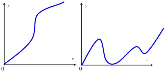
Figure 1.
The possible responses of the solution .
Therefore, it can be claimed that the state remains positive and does not escape within any given finite time . Since the state will not blow up on the time interval , by specifying controller with Equation (36), we can utilize a backstepping control design to produce a controller for the original x system in Equation (1). Then, from a result like that in Equation (35), we can conclude that the state x will not blow up on the time interval . Since , the system controllers and can be switched into Equations (8) and (34) at time , respectively.
Now, in this moment, we are ready to summarize the main result of this section in the following theorem:
Theorem 1.
Suppose that Assumptions 1 and 2 hold. If the control scheme is actuated to the system in Equation (1) in such a way that (1) when , and and (2) when , and , then the uncertain system in Equation (1) is asymptotically stable, while the full-state constraints are not violated by choosing appropriate parameters.
Proof.
By choosing the entire BLF , one has . Since and , by using the proof process of Proposition 1, it can be proven that and are bounded, and meanwhile, and . By applying the well-known LaSalle’s invariant theorem, it follows that tends toward the largest invariant set contained in the set where . This fact in turn implies that and as . Note that all the virtual control variables once . The above stability analysis results further indicate that and as . Accordingly, one can show that and as . Now, we will demonstrate how the desired full-state constraints are guaranteed. From Proposition 1, it holds readily that can be obtained directly by choosing . Since , in light of Equation (10), we have . Hence, by choosing , one has . By using a similar proof process, we can prove in an orderly manner that , . □
3. Adaptive Stabilization of Nonholonomic Uncertain Systems
In this section, we investigate a classical kind of uncertain nonholonomic system whose model is expressed as
where represents the system state vector, ’s denote the smooth nonlinear function vectors, stands for an unknown bounded constant parameter vector, and and are the system control inputs.
The control objective of this part is to design the adaptive stabilization control laws and of the form , , and such that all states of the system in Equation (39) converge to zero asymptotically while the aforementioned full-state constraints are not violated. To achieve this aim, the assumption imposed on the system in Equation (39) is expressed as follows:
Assumption 3.
We assume that there is a smooth known function vector such that
For each , there exists a smooth known function vector such that
3.1. State Transformations
Assumption 3 implies that the system in Equation (39) possesses a triangularity structure. To clearly grasp the essence of the control design, the case where is studied first. Then, the case of will be discussed in Section 3.3.
For the subsystem, we consider the following BLF:
where denotes a positive definite matrix, , and represents the first on-line estimation of . Therefore, the control input is designed such that
and the adaptive law is defined as
with . Under Equations (43) and (44), the time derivative of is computed as follows:
From Equation (45), we know that and are bounded, and , as , provided that . With the designed control law in Equation (43), the resulting closed-loop subsystem can be formulated as follows:
3.2. Tuning Function Design
To design the adaptive control law , the tuning function is presented step by step as follows. As usual, the recursive design begins with a simple subsystem and then goes on to a higher-order system, and it ultimately stops once the actual input occurs.
Step 1: We introduce and , where is referred to as the first virtual control which is used to stabilize the subsystem. Now, we choose the first BLF to be
where are positive constants and denotes a positive definite matrix. In this step, it is easy to determine the virtual control and tuning function to be
Then, we can find that
Step i : We consider the BLF to be with and define and
In this step, the virtual control and tuning function are designed as follows:
where
which generates the following results:
At the last step, the actual control law and adaptive law are specified as follows:
and
3.3. Adaptive Switching and the Main Results
In the aforementioned discussion, we completed the control development when . Next, we will present the control design procedure for and in the case where . When , like in [33], we design as follows:
where is defined by Equation (43). Considering the same BLF (Equation (42)) and adaptive law (Equation (44)), we can have
where positive constants and are chosen to satisfy and . Returning to Equation (62), it can be seen that is negative once . Hence, as long as , and are bounded, moreover, for any . Under Equation (61), the closed-loop subsystem is described as follows:
Under Equation (63), by using the same arguments as in Section 2.3, we can conclude that for any given finite time , state remains positive and does not escape. Once when , the control input is switched from Equation (61) into Equation (43). Consequently, the state scaling can be carried out for the upcoming control development.
On the time interval , under (defined by Equation (61)), using backstepping-based state feedback, and an another adaptive law can be designed by a similar control procedure (presented in Section 3.2) to the original x system in (39). Then, it can be claimed that state x will not blow up during the time period . Note that when , and the control inputs and are switched into Equations (43) and (58), respectively.
Now, the main result of this section is included in the following theorem:
Theorem 2.
Suppose that Assumption 3 holds for the system in Equation (39). If the control input in Equation (43) and the state feedback control input in Equation (58) are applied to the system in Equation (39) with the adaptive laws in Equations (44) and (59) along with the aforementioned adaptive switching strategy, then the uncertain system in Equation (39) is globally asymptotically stable while the full-state constraints are not violated.
Proof.
The proof of Theorem 2 is similar to that of Theorem 1. Therefore, it was omitted here to avoid duplication. □
Remark 5.
In adaptive stabilization control, the viscous friction term can be considered since it is linearly dependent on the physical parameters. For example, let us consider the model of viscous friction to be . Then, this friction can be rewritten into a compact form with and , which can be treated with the proposed adaptive stabilization control approach.
4. Simulation Results
In this part, we will demonstrate the effectiveness of the systematic stabilization control law design methods proposed above through two examples.
Example 1.
The first considered example is the tricycle-type mobile robot with parametric uncertainty [4]:
where represents the coordinate of the mass center, θ represents the heading angle, v and ω stand for the forward linear velocity and the angular velocity, respectively, and the parameters take values in a known interval with .
Next, we will show that the system in Equation (64) can be transformed into an equivalent system characterized by Equation (1), subject to Assumptions 1 and 2. Now, under the following state and input transformations
the system in Equation (64) is reformulated as
which belongs to the type from Equation (1). Assume that . By applying the controller design in Section 2.1 and Section 2.2, we have
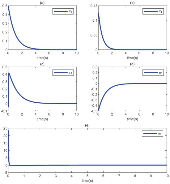
where , , , , , , , , , and .
To proceed with the simulation, the system parameters were chosen to be , , , and . The control design parameters were configured to be , , and . The initial conditions were designed to be , , and . The simulation results are provided in Figure 2. After a careful look at all the subgraphs in Figure 2, all the closed-loop system signals converged to zero as the time approached infinity. Obviously, the desired state constraints were not violated since all system states decayed to zero with no fluctuation. The simulation results are consistent with the theoretical analysis.
Figure 2.
The responses of the closed-loop system (66). (a) , (b) , (c) , (d) is the system control inputs, (e) is the system control inputs.
Example 2.
To illustrate the validity of the adaptive stabilization control law, we consider the following numerical example:
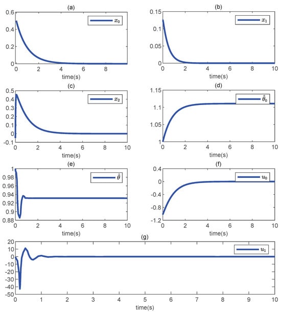
where is the system state vector, θ denotes the unknown parameter, and and are the system control inputs. By applying the controller design in Section 3.1 and Section 3.2, one has
where , , , , and . For the simulation, we chose , , , , , , , , and . The initial system conditions were designed to be , , , , and . The simulation results are shown in Figure 3. From Figure 3, it can be easily seen that the closed-loop system signals tended toward zero as . Meanwhile, the adaptive law converged to its own steady state. In addition, the desired state constraints were also not violated, since all system states decayed to zero with no fluctuation. The simulation results are satisfactory in terms of work efficiency.
Figure 3.
The responses of the closed-loop system (68). (a) , (b) , (c) , (d) , (e) , (f) is the system control inputs, (g) is the system control inputs.
5. Conclusions
Two recursive BLF techniques have been developed for the stabilization control for a strict-feedback nonholonomic system. It is crucial to mention that the designed stabilization control techniques are analytically simple and guarantee that the system states can be regulated to zero asymptotically while the full-state constraints are not violated. The validity of the stabilization control strategies is illustrated through two examples of chained-form nonholonomic systems, namely the tricycle-type mobile robot with parametric uncertainty and a numerical example.
Author Contributions
Conceptualization, Z.Z.; methodology, Z.Z.; validation, Z.Z.; writing—original draft preparation, X.H. (Xueli Hu) and Y.G.; writing—review and editing, X.H. (Xiaodan Hou). All authors have read and agreed to the published version of the manuscript.
Funding
This research was funded partly by the National Natural Science Foundation of China under Grant 62173207, the China Postdoctoral Science Special Foundation under Grant 2023T160334, the Youth Innovation Team Project of Colleges and Universities in Shandong Province under Grant 2022KJ176, and the Graduate Teaching Case Base Project of Shandong Province under Grant SDYAL20109.
Data Availability Statement
No new data were created or analyzed in this study. Data sharing is not applicable to this article.
Conflicts of Interest
The authors declare no conflict of interest.
Appendix A
Proof of Proposition 2.
In the proof of Equation (24) in Section 2.2, it has been proven that
where is a nonnegative function.
Next, like in [40], we will use an inductive argument to show that the result of Proposition 1 holds. To this end, we make the following inductive assumption: for , there are functions such that
In what follows, our goal is to show that there are functions such that
First, we address the cases where is considered. Recalling that and , in light of Equation (A2), it can be verified that
with being functions.
Now, it will be proven that Equation (A4) also holds for . Since , and is independent on , one has
where is a function. Therefore, due to Equations (A4) and (A5), we know that Equation (A3) is true. In addition, through Equations (14) and (16), one has
where is a function. By combining Equation (A3) with Equation (A6), this yields that for , we have
where are functions. Up to now, under Equation (A7), it follows readily that
where is a function. The proof of Proposition 2 is completed. □
References
- Murray, R.M.; Sastry, S. Nonholonomic motion planning: Steering using sinusoids. IEEE Trans. Autom. Control. 1993, 38, 700–716. [Google Scholar] [CrossRef]
- Wu, Y.Q.; Wang, B.; Zong, G.D. Finite-time tracking controller design for nonholonomic systems with extended chained form. IEEE Trans. Circuits Syst. 2005, 52, 798–802. [Google Scholar]
- Brockett, R.W.; Millman, R.S.; Sussmann, H.J. Differential Geometric Control Theory; Birkauser: Boston, MA, USA, 1983. [Google Scholar]
- Jiang, Z.P. Robust exponential regulation of nonholonomic systems with uncertainties. Automatica 2000, 36, 189–209. [Google Scholar] [CrossRef]
- Tian, Y.P.; Li, S.H. Exponential stabilization of nonholonomic systems by smooth time-varying control. Automatica 2002, 38, 1139–1146. [Google Scholar] [CrossRef]
- Luo, J.; Tsiotras, P. Control design for chained-form systems with bounded inputs. Syst. Control Lett. 2000, 39, 123–131. [Google Scholar] [CrossRef]
- Zhao, Y.; Yu, J.B.; Wu, Y.Q. State-feedback stabilization for a class of more general high order stochastic nonholonomic systems. Int. J. Adapt. Control Signal Process. 2011, 25, 687–706. [Google Scholar] [CrossRef]
- Do, K.D. Global inverse optimal stabilization of stochastic nonholonomic systems. Syst. Control Lett. 2015, 75, 41–45. [Google Scholar] [CrossRef]
- Ou, M.Y.; Du, H.B.; Li, S.H. Finite-time formation control of multiple nonholonomic mobile robot. Int. J. Robust Nonlinear Control 2014, 24, 140–165. [Google Scholar] [CrossRef]
- Gao, F.; Huang, J.; Shi, X.; Zhu, X. Nonlinear mapping-based fixed-time stabilization of uncertain nonholonomic systems with time-varying state constraints. J. Frankl. Inst. 2020, 357, 6653–6670. [Google Scholar] [CrossRef]
- Huang, J.S.; Wen, C.Y.; Wang, W.; Jiang, Z.P. Adaptive stabilization and tracking control of a nonholonomic mobile robot with input saturation and disturbance. Syst. Control Lett. 2013, 62, 234–241. [Google Scholar] [CrossRef]
- Jenabzadeh, A.; Safarinejadian, B. Distributed tracking of nonholonomic targets over multiagent systems. IEEE Syst. J. 2019, 13, 1678–1681. [Google Scholar] [CrossRef]
- Sun, Z.; Dai, L.; Xia, Y.; Liu, K. Event-based model predictive tracking control of nonholonomic systems with coupled input constraint and bounded disturbances. IEEE Trans. Autom. Control 2018, 63, 608–615. [Google Scholar] [CrossRef]
- Kim, B.S.; Yoo, S.J. Adaptive control of nonlinear pure-feedback systems with output constraints: Integral barrier Lyapunov functional approach. Int. J. Control Autom. Syst. 2015, 13, 249–256. [Google Scholar] [CrossRef]
- Liu, Y.J.; Tong, S.C. Barrier Lyapunov functions-based adaptive control for a class of nonlinear pure-feedback systems with full state constraints. Automatica 2016, 64, 70–75. [Google Scholar] [CrossRef]
- Niu, B.; Zhao, J. Tracking control for output-constrained nonlinear switched systems with a barrier Lyapunov function. Int. J. Syst. Sci. 2013, 44, 978–985. [Google Scholar] [CrossRef]
- Tee, K.P.; Ge, S.S. Control of nonlinear systems with partial state constraints using a barrier Lyapunov function. Int. J. Control 2011, 84, 2008–2023. [Google Scholar] [CrossRef]
- Xu, Z.B.; Sun, C.B.; Liu, Q.Y. Output-feedback prescribed performance control for the full-state constrained nonlinear systems and its application to DC motor system. IEEE Trans. Syst. Man Cybern. Syst. 2023, 53, 3898–3907. [Google Scholar] [CrossRef]
- He, W.; David, A.O.; Zhao, Y.; Sun, C. Neural network control of a robotic manipulator with input deadzone and output constraint. IEEE Trans. Syst. Man Cybern. Syst. 2016, 46, 759–770. [Google Scholar] [CrossRef]
- Sun, W.; Su, S.-F.; Xia, J.W.; Nguyen, V.T. Adaptive fuzzy tracking control of flexible-joint robots with full-state constraints. IEEE Trans. Syst. Man Cybern. Syst. 2019, 49, 2201–2209. [Google Scholar] [CrossRef]
- Xia, J.W.; Zhang, J.; Sun, W.; Zhang, B.Y.; Wang, Z. Finite-time adaptive fuzzy control for nonlinear systems with full state constraints. IEEE Trans. Syst. Man Cybern. Syst. 2018, 49, 1541–1548. [Google Scholar] [CrossRef]
- Lin, L.X.; Xu, Z.P.; Zheng, J.C. Predefined time active disturbance rejection for nonholonomic mobile robots. Mathematics 2023, 11, 2704. [Google Scholar] [CrossRef]
- Duan, G.R. Brockett’s first example: An FAS approach treatment. J. Syst. Sci. Complex. 2022, 35, 441–456. [Google Scholar] [CrossRef]
- Duan, G.R. Brockett’s second example: An FAS approach treatment. J. Syst. Sci. Complex. 2023, 36, 1789–1808. [Google Scholar] [CrossRef]
- Duan, G.R. Approach for stabilization of generalized chained forms: Part I. discontinuous control laws. Sci. China Inf. Sci. 2023. [Google Scholar] [CrossRef]
- Zhang, Z.C.; Duan, G.R. Stabilization controller of an extended chained nonholonomic system with disturbance: An FAS approach. IEEE/CAA J. Autom. Sin. 2023. [Google Scholar] [CrossRef]
- Zhang, S.M.; Gao, Y.; Zhang, Z.C.; Cao, D.G. SDF-based tracking control for state-constrained nonholonomic systems with disturbances via relay switching control: Theory and experiment. Int. J. Adapt. Control Signal Process. 2022, 36, 852–869. [Google Scholar] [CrossRef]
- Zhang, Z.C.; Bian, J.S.; Wu, K. Relay-switching-based fixed-time tracking control for state-constrained nonholonomic systems: Design and experiment. IEEE/CAA J. Autom. Sin. 2023, 10, 1778–1780. [Google Scholar] [CrossRef]
- Liu, M.M.; Wu, K.; Wu, Y.Q. Finite-time tracking control of disturbed non-holonomic systems with input saturation and state constraints: Theory and experiment. IET Control Theory Appl. 2023, 17, 1663–1676. [Google Scholar] [CrossRef]
- Zhang, Z.C.; Cheng, W.L.; Wu, Y.Q. Trajectory tracking control design for nonholonomic systems with full-state constraints. Int. J. Control Autom. Syst. 2021, 19, 1798–1806. [Google Scholar] [CrossRef]
- Du, Q.; Wang, L.; Zhao, C. Adaptive neural control for stochastic nonholonomic systems with full-state constraints and unknown covariance noise. Appl. Anal. 2023, 102, 1914–1933. [Google Scholar] [CrossRef]
- Ju, S.; Wang, J.; Dou, L. MPC-based cooperative enclosing for nonholonomic mobile agents under input constraint and unknown disturbance. IEEE Trans. Cybern. 2022, 53, 845–858. [Google Scholar] [CrossRef] [PubMed]
- Zhang, Z.C.; Zhang, S.M.; Wu, Y.Q. New stabilization controller of state-constrained nonholonomic systems with disturbances: Theory and experiment. IEEE Trans. Ind. Electron. 2023, 70, 669–677. [Google Scholar] [CrossRef]
- Gao, F.; Huang, J.; Zhu, X.; Wu, Y. Output feedback stabilization via nonlinear mapping for time-varying constrained nonholonomic systems in prescribed finite time. Inf. Sci. 2021, 550, 297–312. [Google Scholar] [CrossRef]
- Wu, Y.; Wang, Y.; Fang, H.; Wan, F. Cooperative learning control of uncertain nonholonomic wheeled mobile robots with state constraints. Neural Comput. Appl. 2021, 33, 17551–17568. [Google Scholar] [CrossRef]
- Ge, S.S.; Wang, Z.P.; Lee, T.H. Adaptive stabilization of uncertian nonholonomic systems by state and output feedback. Automatica 2003, 39, 1451–1460. [Google Scholar] [CrossRef]
- Sun, W.; Su, S.F.; Dong, G.; Bai, W. Reduced adaptive fuzzy tracking control for high-order stochastic nonstrict feedback nonlinear system with full-state constraints. IEEE Trans. Syst. Man Cybern. Syst. 2019, 51, 1496–1506. [Google Scholar] [CrossRef]
- Khalil, H.K. Nonlinear Systems; Prentice-Hall: Hoboken, NJ, USA, 2002. [Google Scholar]
- Arnold, V.I. Geometrical Methods in the Theory of Ordinary Differential Equations; Springer: Berlin/Heidelberg, Germany, 1987. [Google Scholar]
- Huang, X.Q.; Lin, W.; Yang, B. Global finite-time stabilization of a class of uncertain nonlinear systems. Automatica 2005, 41, 881–888. [Google Scholar] [CrossRef]
Disclaimer/Publisher’s Note: The statements, opinions and data contained in all publications are solely those of the individual author(s) and contributor(s) and not of MDPI and/or the editor(s). MDPI and/or the editor(s) disclaim responsibility for any injury to people or property resulting from any ideas, methods, instructions or products referred to in the content. |
© 2023 by the authors. Licensee MDPI, Basel, Switzerland. This article is an open access article distributed under the terms and conditions of the Creative Commons Attribution (CC BY) license (https://creativecommons.org/licenses/by/4.0/).