Design and Analysis of an Individual-Based Model for Malware Propagation on IoT Networks

Abstract

The main goal of this work is to propose a novel compartmental SEA (Susceptible–Exposed–Attacked) model to simulate malware spreading on an IoT (Internet of Things) network. This is a deterministic and individual-based model, whose main novelty compared to others lies in the used of continuous mathematical techniques, such as ordinary differential equations, in the description of local transition rules that define the changes of the states of the devices. These states are given by probability vectors representing the probabilities of being susceptible, exposed and attacked at each step of time. The qualitative study of the model is presented, and several simulations are performed.

1. Introduction

The Internet of Things (IoT for short) has rapidly evolved into a pervasive technological paradigm, characterized by the interconnection of a wide range of physical devices, such as sensors, computers, and software, for monitoring and control that facilitate data exchange and intelligent and autonomous decision making. The most important attributes that define IoT include its ability to collect real-time data from the physical world, enabling automation, enhanced efficiency, and improved quality of life. In this sense, IoT spans various domains, including Industry 4.0, smart homes, e-health, intelligent transport systems, and smart cities [1,2,3,4].

However, in this scenario of unprecedented and ubiquitous connectivity, we have to face great challenges, chief among them being the evolving cyber threats, with malware emerging as a significant concern [5,6,7]. In this context, the different specimens of malware can infiltrate devices, compromise data integrity, disrupt operations and network functionalities, and even compromise personal privacy and security. Thus, it is very important to design tools that allow not only to detect the presence of malware on the network but also to predict its future behavior. As a consequence, to counteract the malicious activity of malware in IoT environments, it is crucial to distinguish between these two key aspects: malware detection algorithms and malware propagation models. Malware detection algorithms are focused on identifying and mitigating malware infections within devices and networks [8,9]. In contrast, malware propagation models are responsible for studying the dynamics of malware spreading through interconnected devices.

Mathematical epidemiology traditionally deals with the mathematical description and analysis of the dissemination of biological agents. Drawing inspiration from it, several models for malware propagation on different types of networks have appeared in recent years. Particularly interesting are those dedicated to study the propagation of malicious code on wireless sensor networks (WSNs), which constitute the foundation for the development and implementation of IoT networks. The vast majority of these models are of a global nature (see, for example, [10,11,12,13,14] and the references therein), and their dynamics are described by continuous mathematical techniques, such as systems of ordinary differential equations. These are compartmental models (that is, the device population is divided into different classes or compartments: susceptible, infectious, recovered, etc.), and the main goal is to determine the temporal evolution of the size of these compartments. Consequently, the variables involved in the differential equations (that govern the dynamics of the system) represent the density at each step of time of susceptible devices, infectious devices, etc. Additionally, the epidemiological coefficients considered in these equations are inevitably of a general nature, making it impossible to distinguish between devices in a particular compartment. Moreover, it is not feasible to consider the local contact topology such that in the majority of models it is assumed that the communication topology is defined by means of a complete graph (all devices are in contact with all). Nevertheless, it is also true that it is possible to design models (networked models) where the degree distribution of the complex network defining the contact topology can be considered when defining the incidence term (see, for example, [15,16,17]). Consequently, a critical analysis of global models reveals certain limitations that overlook the intricate topological structures of IoT networks and the heterogeneity of individual devices ([18,19]). This limitation necessitates a shift toward individual-based models, which consider the unique attributes of each network node [20,21].

The use of individual-based models for malware propagation presents a promising research line, offering a more detailed and realistic representation of malware dissemination on IoT networks. While this approach has gained traction, the state of the art concerning individual-based models for malware propagation, especially in the context of IoT networks, remains an area of active investigation. As far as we know, very few individual-based models for malware propagation have been proposed. In [22], an individual-based, discrete, and stochastic SEIRS-F model is proposed. The authors aim to analyze malware propagation in a wireless sensor network and investigate the reliability of its components in this scenario. In [23], an SITPS stochastic compartmental model is studied and analyzed, introducing—in addition to the classic compartments of susceptible and infected—the compartments of “tracked” (T) and “repaired” (P) devices. In [24], an agent-based SEIRD model is described, providing a detailed analysis of all the characteristics of the agents involved in the propagation. In [25], an individual-based model is proposed such that the dynamics of the malware outbreak is governed by means of a cellular automaton. In all these models, the variables involved in the transition functions correspond to the states of the particular devices, in contrast to what happens in global models, where the variables stand for the size of each compartment.

The use of mathematical models based on the individual paradigm is especially indicated when it is possible to have a deep knowledge of the interactions and specific characteristics of the potential hosts among which the agent (of whatever type) spreads. In the case of the propagation of biological agents, this type of model could be appropriate when, for example, the spread of a nosocomial infection is studied in an intensive care unit—note that patients are permanently monitored and it is possible to have a fairly approximate idea of their interactions. In other types of broader and more general scenarios in which a biological agent is spread, it would not be worthwhile to use individual models: global models would work perfectly well. In the case at hand, when the propagation is due to a “logical” agent (malicious code) on a network of computer devices (where it is possible to monitor the different devices in real time and know their activities, capabilities and objectives), it is reasonable to advocate for the use of individual models. Specifically, in the case of IoT device networks, different types of metrics can be applied to measure useful characteristics in the propagation process. For example, the communication capabilities and computational resources of the devices can give us an idea (both in terms of quality and performance) of how the devices can be used in the propagation process, how the specific task of a device will determine whether it is a target to attack or not, how the energy sources associated to a device will determine its lifetime, etc.

The main goal of this paper is to propose and analyze a novel individual-based model to predict the behavior of a specimen of malware on an IoT network. This is a compartmental SEA model, where the population of devices is classified into susceptible, exposed and attacked, and the dynamics refers to the variation of the states of devices at each step of time. These states are given by probability vectors such that the transition is ruled by a system of ordinary differential equations. This definition of the state for each device is what sets this model apart from the other individual models we previously mentioned. With it, it becomes possible to use differential equations as transition rules instead of cellular automata or other discrete tools.

The rest of the paper is organized as follows: in Section 2, the fundamentals of individual-based modeling for malware propagation are stated; the proposed model is introduced and analyzed in Section 3; and the conclusions are shown in Section 4.

2. The Individual-Based Paradigm

Individual-based modeling is based on the study of the behavior of the individuals/agents that constitute the system, taking into account their particular characteristics. In the case at hand, these agents stand for the devices deployed within the IoT network and the specimen of malware. Therefore, as previously mentioned, the development of individual-based mathematical models for malware propagation on IoT networks necessitates a consideration of two key aspects: the specific attributes of devices and the specimen of malware pertaining to propagation and infection processes, and the unique contact topology, often leading to the consideration of a complex network structure.

In this context, the scenario can be succinctly characterized through a directed and weighted complex network denoted as $\mathcal{G}=\left(\mathcal{V},\mathcal{E}\right)$. Here, the set of nodes $\mathcal{V}=\{v_1,\dots ,v_n\}$ symbolizes the population of devices, and the links stand for the communication connections among these devices. The dynamics of malware propagation is thus defined by the following components:

(1)

The state of the i-th device at time t, which is denoted as $s_i^t$. In this sense, time can flow both continuously or at discrete steps of time.

(2)

The state set $\mathcal{S}$, within which the aforementioned individual states take their values: $s_i^t\in \mathcal{S}$ for $t>0$ and $1\le i\le n$. This set can be finite, allowing devices to assume a finite number of possible states at each time step, or it can be infinite so that the states are continuous in nature: for example, $s_i^t\in [0,1]$.

(3)

Device states evolve in discrete time steps, following local transition rules that are defined by means of continuous or discrete, deterministic or stochastic mathematical tools.

Consequently, several types of local transition functions can be used to describe the dynamics of the individual states. In our case, we will propose an individual-based model, where the states stand for stochastic vectors that take continuous values and the time flows also in a continuous way.

3. The Proposed Individual-Based Model

In this section, the novel individual-based model for malware propagation on an IoT network is introduced and analyzed. As is previously mentioned, it is a compartmental SEA model, where population is divided into susceptible S, exposed E, and attacked A devices. It is assumed that a susceptible device becomes exposed when the specimen of malware reaches it and carries out the decision process to determine whether to attack the host device (making it “attacked”) or propagate to a neighbor device, returning the host to a state of susceptibility. Note that infectious devices are those which are exposed. Furthermore, attacked devices remain in this state indefinitely (see Figure 1).

3.1. Mathematical Formulation of the Model

As is mentioned in Section 2, the IoT network can be mathematically characterized as a directed and weighted complex network: $\mathcal{G}=\left(\mathcal{V},\mathcal{E}\right)$, where the set of nodes $\mathcal{V}$ represents the population of devices (the i-th node is given by $v_i\in \mathcal{V}$), and the set of edges $\mathcal{E}$ stands for the direct communication links between two devices (if the i-th node $v_i$ can transmit information to the j-th node $v_j$, then $e_{ij}=\left(v_i,v_j\right)\in \mathcal{E}$).

Set ${\mathcal{N}}_i^{\mathrm{in}}$ to the in-neighborhood of the i-th node, that is, the set of adjacent nodes to $v_i$:

$${\mathcal{N}}_i^{\mathrm{in}}=\{v_j\in \mathcal{V}:e_{ji}=\left(v_j,v_i\right)\in \mathcal{E}\}=\{v_{j_1},\dots ,v_{j_{k_i^{\mathrm{in}}}}\}\subset \mathcal{V}.$$

(1)

Moreover, the out-neighbor of $v_i$ can be defined similarly as the set of adjacent nodes from $v_i$:

$${\mathcal{N}}_i^{\mathrm{out}}=\{v_j\in \mathcal{V}:e_{ij}=\left(v_i,v_j\right)\in \mathcal{E}\}=\{v_{i_1},\dots ,v_{i_{k_i^{\mathrm{out}}}}\}\subset \mathcal{V}.$$

(2)

Note that ${\mathcal{N}}_i^{\mathrm{in}}\cap {\mathcal{N}}_i^{\mathrm{out}}$ is the set of devices with which the i-th device has a two-way communication.

Each link $e_{ij}=\left(v_i,v_j\right)\in \mathcal{E}$ of the network is endowed with a weight $w_{ij}\in [0,1]$ representing the strength of infection from the i-th device to the j-th device: if $w_{ij}=0$, then it is impossible for the specimen of malware hosted in $v_i$ to reach the device $v_j$, whereas if $w_{ij}=1$, then the malware spreads successfully from the i-th node to the j-th node at every step of time and contact. Specifically, $w_{ij}=c_{ij}·q_{ij}$ where $c_{ij}$ is the number of communication contacts from $v_i$ to $v_j$ per unit of time, and $0\le q_{ij}\le 1$ is the probability that a communication contact leads to a “contagion”. Consequently, the adjacency matrix associated to $\mathcal{G}$, $A={\left(a_{ij}\right)}_{1\le i,j\le n}$ can be defined as follows:

$$a_{ij}=\left\{\begin{array}{cc}0,\hfill & \mathrm{if}{e}_{ij}\notin \mathcal{E}\hfill \\ w_{ij}\in [0,1],\hfill & \mathrm{otherwise}\hfill \end{array}\right.$$

(3)

As the proposed model follows the individual-based paradigm, the variables of the equations that describe the dynamics stand for the states of the devices at every time. In this sense, the state of the i-th device at time t is defined as $s_i^t=\left(x_i\left(t\right),y_i\left(t\right),z_i\left(t\right)\right)\in [0,1]\times [0,1]\times [0,1]$, where $x_i\left(t\right)$ represents the probability that the i-th device is susceptible at t, $y_i\left(t\right)$ stands for the probability that the i-th device is exposed at t, and finally, $z_i\left(t\right)=1-x_i\left(t\right)-y_i\left(t\right)$ is defined as the probability of the i-th device being attacked at t.

Let

$${\mathcal{I}}_i\left(t\right)=\{v_{j_l}\in {\mathcal{N}}_i^{\mathrm{in}}:y_{j_l}\left(t\right)>0,z_{j_l}\left(t\right)=0\}\subseteq {\mathcal{N}}_i,$$

(4)

be the set of in-neighbor devices to $v_i\in \mathcal{V}$ such that its probability of being infectious at t is greater than 0, and its probability of being attacked at t is 0. Then, the dynamics of the system is described by means of the following system of ordinary differential equations:

$$\begin{array}{ccc}\hfill x_i^{\prime }\left(t\right)& =& -\sum _{v_{jl\in {\mathcal{I}}_i\left(t\right)}}{w}_{j_{l}i}{x}_i\left(t\right)y_j\left(t\right)+{\gamma }_i{y}_i\left(t\right),1\le i\le n,\hfill \end{array}$$

(5)

$$\begin{array}{ccc}\hfill y_i^{\prime }\left(t\right)& =& \sum _{v_{jl\in {\mathcal{I}}_i\left(t\right)}}{w}_{j_{l}i}{x}_i\left(t\right)y_j\left(t\right)-\left({\beta }_i+{\gamma }_i\right)y_i\left(t\right),1\le i\le n,\hfill \end{array}$$

(6)

$$\begin{array}{ccc}\hfill z_i^{\prime }\left(t\right)& =& {\beta }_i{y}_i\left(t\right),1\le i\le n,\hfill \end{array}$$

(7)

or, equivalently, by the following initial value problem (IVP) expressed in terms of the adjacency matrix associated to $\mathcal{G}$:

$$\begin{array}{ccc}\hfill x_i^{\prime }\left(t\right)& =& -\sum _{v_j\in \mathcal{V}}{a}_{ji}{x}_i\left(t\right)y_j\left(t\right)+{\gamma }_i{y}_i\left(t\right),1\le i\le n,\hfill \end{array}$$

(8)

$$\begin{array}{ccc}\hfill y_i^{\prime }\left(t\right)& =& \sum _{v_j\in \mathcal{V}}{a}_{ji}{x}_i\left(t\right)y_j\left(t\right)-\left({\beta }_i+{\gamma }_i\right)y_i\left(t\right),1\le i\le n,\hfill \\ \hfill \end{array}$$

(9)

$$\begin{array}{ccc}\hfill z_i^{\prime }\left(t\right)& =& {\beta }_i{y}_i\left(t\right),1\le i\le n,\hfill \end{array}$$

(10)

$$\begin{array}{ccc}& & x_i\left(t\right)+y_i\left(t\right)+z_i\left(t\right)=1,1\le i\le n,\hfill \\ & & x_i\left(0\right)=x_i^0,y_i\left(0\right)=y_i^0,z_i\left(0\right)=1-x_i^0-y_i^0,1\le i\le n,\hfill \end{array}$$

(11)

where ${\gamma }_i$ stands for the recovery coefficient (from exposed to susceptible), and ${\beta }_i$ represents the attack coefficient (transition from exposed to attacked).

As the state of each device is a probabilistic vector (Equation (11)), this IVP of $3n$ ordinary differential equations can be reduced to the following IVP formed by $2n$ ordinary differential equations:

$$\begin{array}{ccc}\hfill x_i^{\prime }\left(t\right)& =& -\sum _{v_j\in \mathcal{V}}{a}_{ji}{x}_i\left(t\right)y_j\left(t\right)+{\gamma }_i{y}_i\left(t\right),1\le i\le n,\hfill \end{array}$$

(12)

$$\begin{array}{ccc}\hfill y_i^{\prime }\left(t\right)& =& \sum _{v_j\in \mathcal{V}}{a}_{ji}{x}_i\left(t\right)y_j\left(t\right)-\left({\beta }_i+{\gamma }_i\right)y_i\left(t\right),1\le i\le n,\hfill \\ \hfill z_i\left(t\right)& =& 1-x_i\left(t\right)-y_i\left(t\right),1\le i\le n,\hfill \\ & & x_i\left(0\right)=x_i^0,y_i\left(0\right)=y_i^0,1\le i\le n.\hfill \end{array}$$

(13)

If $x\left(t\right)={\left(x_1\left(t\right),\dots ,x_n\left(t\right)\right)}^{⊺}\in {[0,1]}^n$ and $y\left(t\right)={\left(y_1\left(t\right),\dots ,y_n\left(t\right)\right)}^{⊺}\in {[0,1]}^n$, the systems (12) and (13) can be expressed in matrix form as follows:

$$\begin{array}{ccc}\hfill x^{\prime }\left(t\right)& =& -\mathrm{diag}\left(x\left(t\right)\right)Ay\left(t\right)+\gamma y\left(t\right),\hfill \end{array}$$

(14)

$$\begin{array}{ccc}\hfill y^{\prime }\left(t\right)& =& \mathrm{diag}\left(x\left(t\right)\right)Ay\left(t\right)-\left(\beta +\gamma \right)y\left(t\right),\hfill \end{array}$$

(15)

where $\gamma =\mathrm{diag}\left({\gamma }_1,\dots ,{\gamma }_n\right)$, and $\beta =\mathrm{diag}\left({\beta }_1,\dots ,{\beta }_n\right)$.

In

Table 1. Symbols and mathematical notation used in the model.

Symbol	Description
$x_i\left(t\right)$	Probability that i-th node is susceptible at t
$y_i\left(t\right)$	Probability that i-th node is exposed at t
$z_i\left(t\right)$	Probability that i-th node is attacked at t
$a_{ji}$	Coefficient $(j,i)$ of the adjacent matrix
$w_{ij}$	Weight associated to the communication link between i-th node and j-th node
$c_{ij}$	Number of contacts between the i-th node and the j-th node per unit of time
$q_{ij}$	Probability that a contact between the i-th and the j-th nodes leads to a contagion
${\beta }_i$	Attack coefficient associated to the i-th node
${\gamma }_i$	Recovery coefficient associated to the i-th node
${\mathcal{N}}_i$	Neighborhood associated to the i-th node
${\mathcal{N}}_i^{\mathrm{in}}$	In-neighborhood of the i-th node at time t
${\mathcal{I}}_i\left(t\right)$	Infected in-neighbors associated to the i-th node at time t

, the most important mathematical notations employed in the model are shown.

3.2. The Underlying Global Model

3.2.1. Mathematical Description and Analysis

Note that the IB model presented in the last subsection is based on the following global model with $x\left(t\right),y\left(t\right),z\left(t\right)\in [0,1]$:

$$\begin{array}{ccc}\hfill x^{\prime }\left(t\right)& =& -wx\left(t\right)y\left(t\right)+\gamma y\left(t\right),\hfill \end{array}$$

(16)

$$\begin{array}{ccc}\hfill y^{\prime }\left(t\right)& =& wx\left(t\right)y\left(t\right)-\left(\beta +\gamma \right)y\left(t\right),\hfill \end{array}$$

(17)

$$\begin{array}{ccc}\hfill z^{\prime }\left(t\right)& =& \beta y\left(t\right),\hfill \end{array}$$

(18)

where $x\left(0\right)=x_0,y\left(0\right)=1-x_0,z\left(0\right)=0$. This system describes the evolution of the particular probabilities of each device in the particular case where the contact topology is defined by the complete graph $\mathcal{G}=K_n$ (that is, all devices are in contact with all devices at every t), and the epidemiological coefficients are all equal: ${\gamma }_i=\gamma \in (0,1],{\beta }_i=\beta \in (0,1]$ for $1\le i\le n$, and $a_{ji}=w$, $1\le i\ne j\le n$.

Since the sum of probabilities must equal to one, $x\left(t\right)+y\left(t\right)+z\left(t\right)=1$ for all t, then the systems (16)–(18) can be reduced to the following:

$$\begin{array}{ccc}\hfill x^{\prime }\left(t\right)& =& -wx\left(t\right)y\left(t\right)+\gamma y\left(t\right),\hfill \end{array}$$

(19)

$$\begin{array}{ccc}\hfill y^{\prime }\left(t\right)& =& wx\left(t\right)y\left(t\right)-\left(\beta +\gamma \right)y\left(t\right),\hfill \end{array}$$

(20)

with $x\left(0\right)=x_0$ and $y\left(0\right)=1-x_0$.

Using simple arguments, the following results can be proved:

Proposition 1.

The region $\mathsf{\Omega }=\{\left(x,y\right)\in [0,1]\times [0,1]:x\ge 0,y\ge 0,x+y\le 1\}$ is positively invariant and unique solutions of the systems (19) and (20) for all $t\ge 0$.

Proposition 2.

The basic reproductive number associated to the epidemiological model described by (19) and (20) is

$${\mathcal{R}}_0=\frac{w}{\beta +\gamma }.$$

(21)

Furthermore, the effective reproductive number (also known as the replacement number) is given by ${\mathcal{R}}_e\left(t\right)={\mathcal{R}}_{0}x\left(t\right)=\frac{wx\left(t\right)}{\beta +\gamma }$. Note that ${\mathcal{R}}_0\ge {\mathcal{R}}_e\left(t\right)$ for every $t\ge 0$.

Theorem 1.

Set $\left(x\left(t\right),y\left(t\right)\right)$ a solution of (19) and (20) in Ω. The following statements hold:

(1)

If ${\mathcal{R}}_e\left(0\right)<1$, then the probability of being exposed decreases to zero, that is: ${lim}_{t\to \infty }\left(x\left(t\right),y\left(t\right)\right)=\left(x_{\infty },0\right)=P_0^{*}$ where $x_{\infty }$ is the unique solution of the following equation:

$$w{x}_{\infty }-\gamma =\left(w{x}_0-\gamma \right)e^{\frac{w}{\beta }\left(x_{\infty }-1\right)}.$$

(22)

(2)

If ${\mathcal{R}}_e\left(0\right)>1$, then the probability of being exposed increases to a maximum value

$$y_{max}=\frac{\beta }{w}log\left(\frac{\beta }{w{x}_0-\gamma }\right)+1-\frac{\beta +\gamma }{w},$$

(23)

and then it decreases to zero such that ${lim}_{t\to \infty }\left(x\left(t\right),y\left(t\right)\right)=P_0^{*}$.

3.2.2. Numerical Simulations

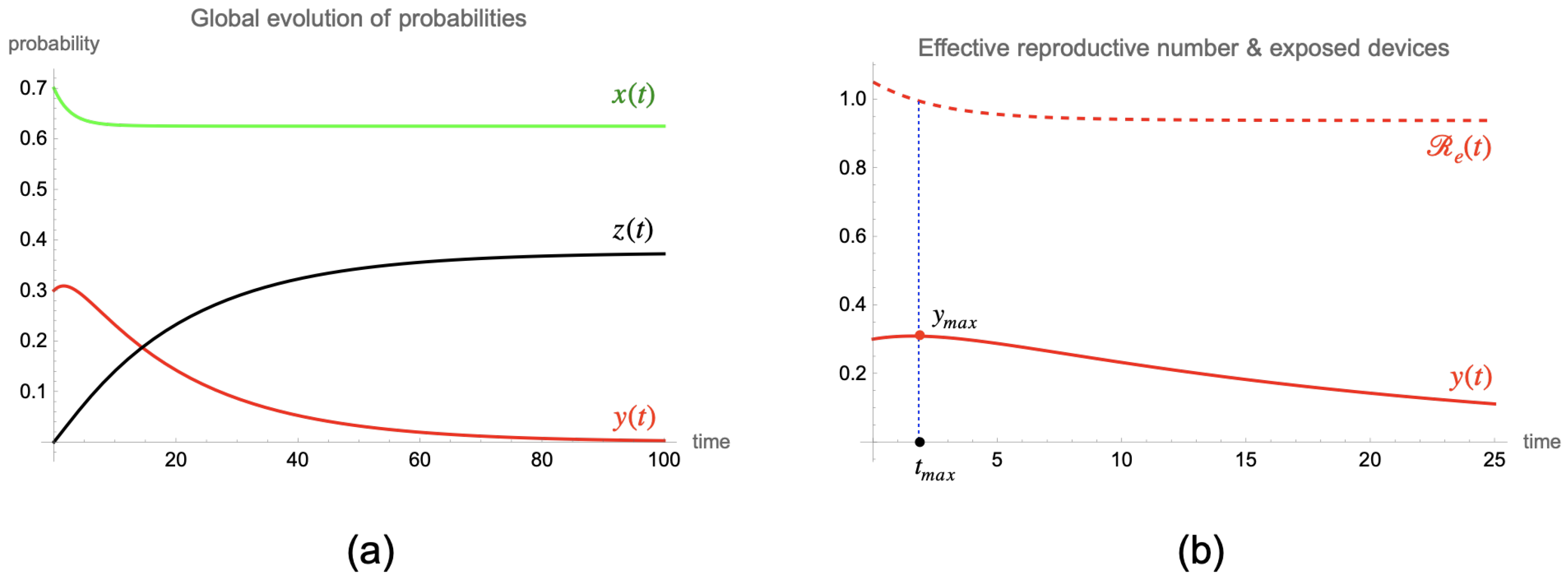
Let us suppose that the numerical values of the epidemiological coefficients are the following: $c=2$, $q=0.6$ (consequently, $w=1.2$), $\gamma =0.75$ and $\beta =0.05$. Moreover, assume that at $t=0$, there is a large fraction of infectious devices: $x_0=0.7$ and $y_0=0.3$. In this case, the basic reproductive number is ${\mathcal{R}}_0=1.5$, whereas the replacement number at $t=0$ is ${\mathcal{R}}_e\left(0\right)\simeq 1.05$. Moreover, the disease-free equilibrium point obtained is $P_0^{*}\simeq \left(0.625,0.003,0.372\right)$.

In Figure 2a, the global evolution of the different probabilities of a (general) device state is shown (susceptible probability in green, exposed probability in red, and attacked probability in black). Note that as ${\mathcal{R}}_e\left(0\right)>1$, then the probability of being exposed initially increases to a maximum $y_{max}\simeq 0.309$, which is reached at $t=t_{max}\simeq 1.723$ (obviously, as you can see in Figure 2b, this occurs when the replacement number decreases to 1, that is, ${\mathcal{R}}_e\left(t_{max}\right)=1$), and then this probability decreases to $y_{\infty }=0$. On the other hand, the probability of being attacked monotonically increases to $z_{\infty }\simeq 0.375$, and the probability of being susceptible monotonically decreases to $x_{\infty }\simeq 0.625$.

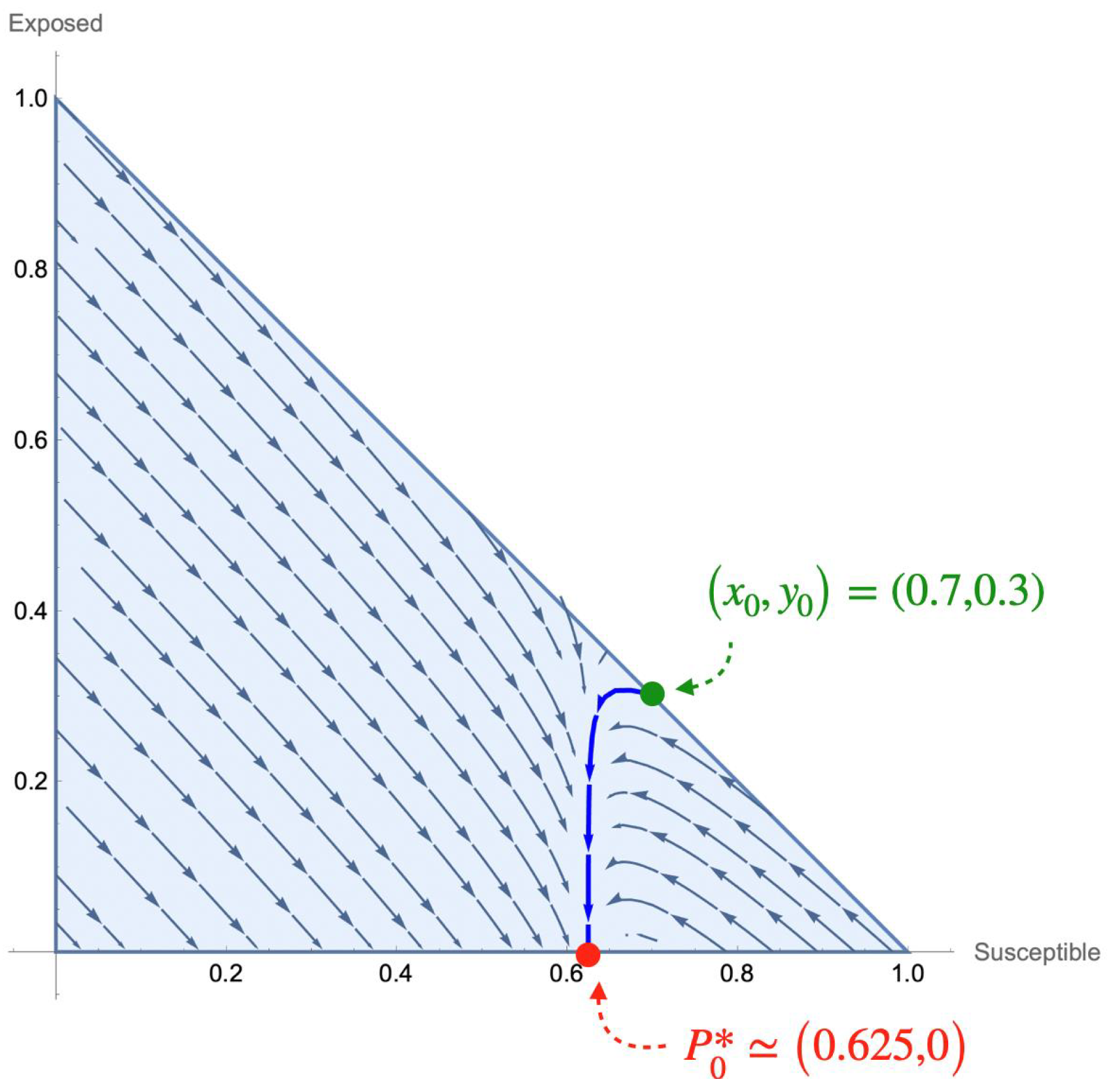
In Figure 3, the phase plane on the feasible region $\mathsf{\Omega }$ for susceptible and exposed probabilities is introduced. Note that, as it has been theoretically proven, all trajectories tend to a disease-free ($y_{\infty }=0$) equilibrium point. Specifically, in this figure, the trajectory corresponding to the solution curve defined by $\left(x_0,y_0\right)$ of the last simulation is highlighted.

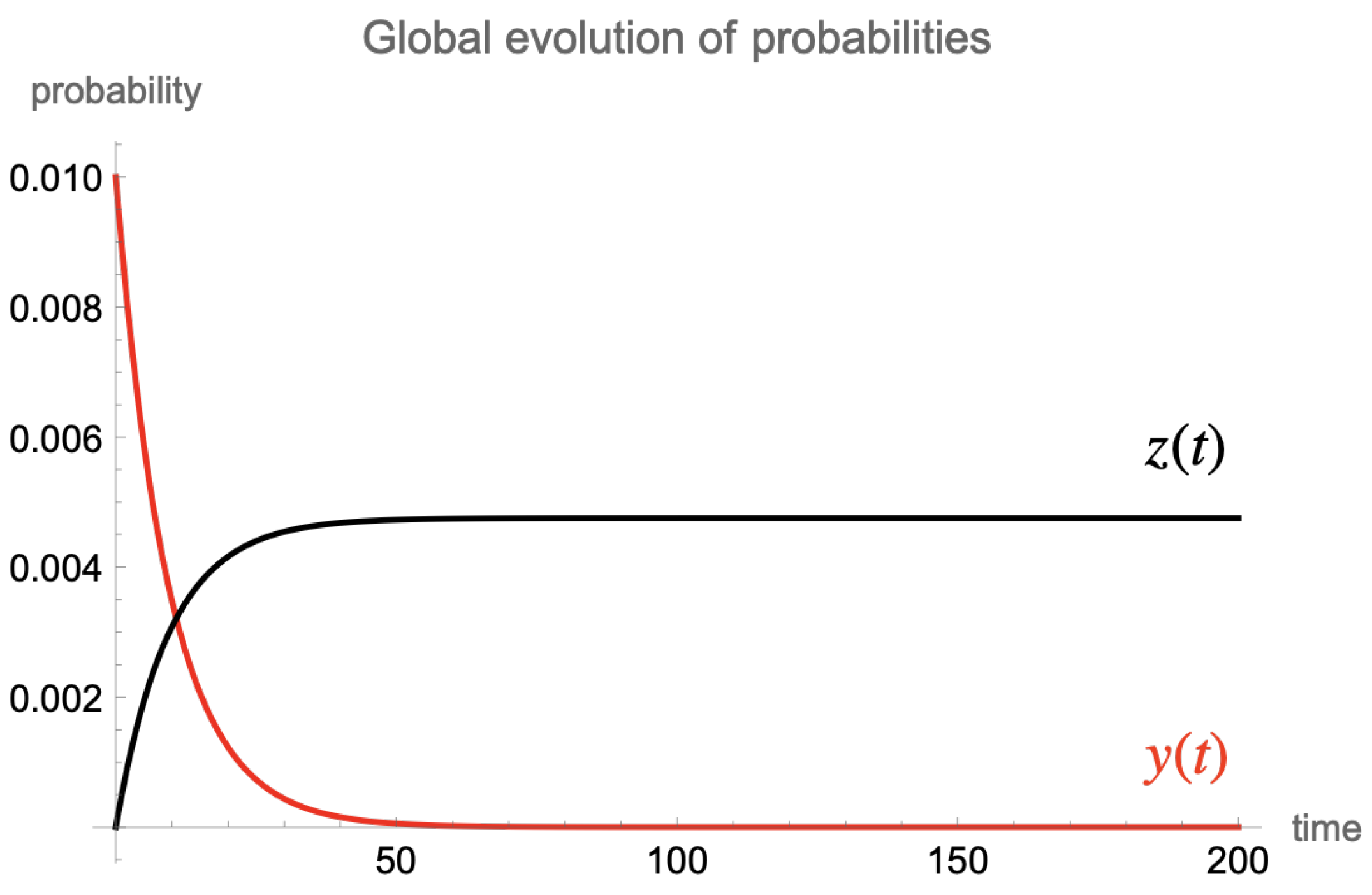
On the other hand, if it is supposed that at $t=0$ the probability of being susceptible is $x_0=0.99$ (and, consequently, $y_0=0.01$), and the contagion probability q is varied to $q=0.35$, then ${\mathcal{R}}_0=0.875<1$ and ${\mathcal{R}}_e\left(0\right)\simeq 0.866<1$. In this situation, the probability of being exposed decreases directly to zero as is illustrated in Figure 4, whereas the probability of being attacked tends to $z_{\infty }=0.005$ and $x_{\infty }=0.995$.

3.2.3. Sensitive Analysis

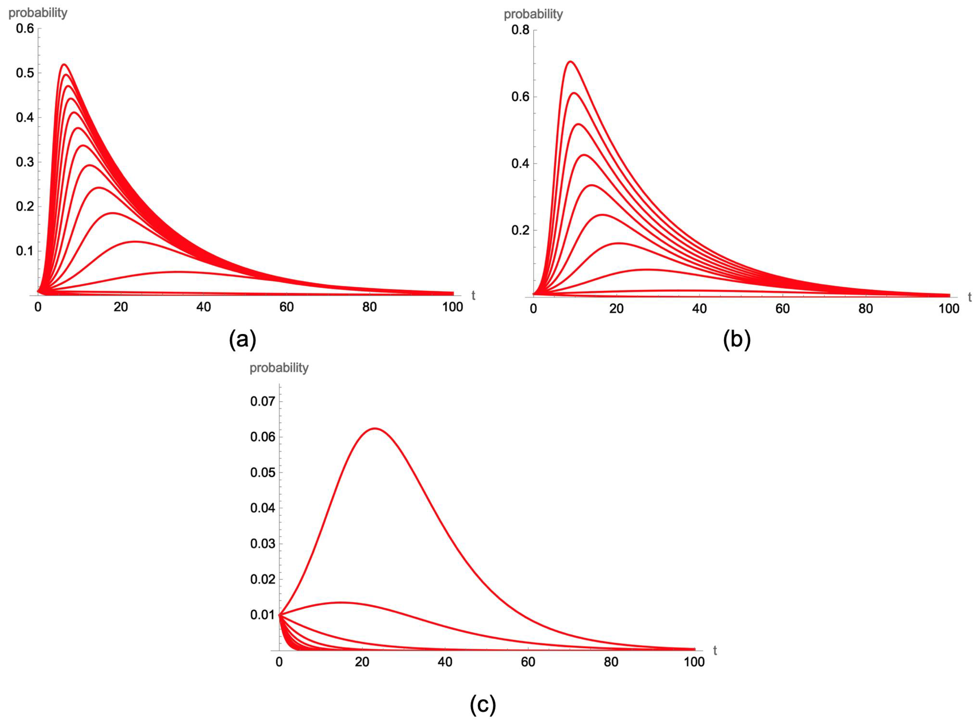
In this subsection, a brief sensitivity analysis of the model is introduced, where slight changes in the numerical value of the three epidemiological coefficients (the infection force w, the recovery coefficient $\beta$, and the attack coefficient $\gamma$) are made.

In Figure 5a, some simulations are shown when the initial conditions are $x_0=0.99$ and $y_0=0.01$, and the values of the epidemiological coefficients are $\gamma =0.75$, $\beta =0.05$, and $w=0.1,0.2,\dots ,1.9,2$. It can be observed that as the infection force increases, the peak of the probability of being exposed also increases. A simple calculation shows that if $w=8$, the basic reproductive number is ${\mathcal{R}}_0=1$ so that if $w>8$, this threshold coefficient is greater than 1, and obviously, the probability curve is monotonically increasing towards the maximum (it will later decrease). On the other hand, in Figure 5b, a similar analysis is carried out, varying, in this case, the numerical value of the recovery coefficient $\gamma =0.1,0.2,\dots ,0.9,1$, and assuming $w=1$ (the rest of the parameters are the same as in the previous case). It is shown that as the recovery coefficient increases, the basic reproductive number decreases: for $\gamma =0.1$, it takes the value ${\mathcal{R}}_0\approx 6.67$; for $\gamma =0.9$, it is ${\mathcal{R}}_0\approx 1.05$; and for $\gamma =1$, it falls below one to ${\mathcal{R}}_{\mathcal{0}}\approx 0.95$. This indicates that the curves corresponding to the probability of being in the exposed state tend to flatten as the recovery coefficient increases. Finally, in Figure 5c, the simulations obtained when varying the attack coefficient $\beta =0.1,0.2,\dots ,0.9,1$ are shown. In this case, it is assumed that $w=1$ and $\gamma =0.75$. Here, as in the previous case, as the attack coefficient increases, the basic reproductive number decreases, finding (in this specific example) that the critical threshold appears at $\beta \approx 0.25$.

3.3. Illustrative Simulations

In this subsection, some illustrative simulations of the proposed individual-based model are shown. Each of them will be characterized by different initial conditions, different contact topologies, and distinct numerical values of the particular epidemiological coefficients: $w_{ij}=c_{ij}·q_{ij},{\gamma }_i$, and ${\beta }_i$ for $1\le i\le n$. More specifically, the simulations are divided into two types: those in which malware spreads on an homogeneous complex network, and those where malware propagates on heterogeneous complex networks.

The simulations are performed in a Mathematica environment using a normal processor (3 GHz Intel Xeon W 10-core). Once all the data related to the topological structure of the network and the epidemiological coefficients involved in the propagation process are processed, a system of $2n$ ordinary differential equations must be solved numerically, where n is the number of nodes. Since the functions to be evaluated in the algorithm defining the numerical method are quite simple, it is known that the computational complexity is polynomial.

3.3.1. Propagation on Homogeneous Networks

In this case, the IoT network is described by means of a homogeneous network: complete network or grid network. With the aim of carrying out a simulation as similar as possible to that given in the case of the global underlying model, it is supposed that all epidemiological coefficients are the same: $c_{ij}=c>1,$ $0\le q_{ij}=q\le 1$, $0\le {\gamma }_i\le 1$, $0\le {\beta }_i\le 1$ for all $1\le i,j\le n$. Specifically, it is assumed that $c_{ij}=1,q_{ij}=0.075,{\gamma }_i=0.85,$ and ${\beta }_i=0.025$, which are the same numerical values considered in the first simulation presented for the underlying global model. Moreover, it is supposed that $n=50$ devices form the networks, and there exists only one exposed device—the “patient zero”—at $t=0$ (that is, $y_i\left(0\right)\ne 0$), which is determined by the highest degree centrality.

If the complete graph is considered, the evolutions of the probabilities of being susceptible ($x_i\left(t\right),1\le i\le n$) exposed ($y_i\left(t\right),1\le i\le n$), and attacked ($z_i\left(t\right),1\le i\le n$) are as shown in Figure 6.

Note that, as it could not be otherwise, the disease-free steady state for all devices is the same: $P_{i,0}^{*}\approx \left(0.231,0,0.769\right)$ with $1\le i\le n$. Moreover, the behavior of the probabilities of all nodes except the one that is initially exposed (say, the j-th node), $x_i\left(t\right),y_i\left(t\right),z_i\left(t\right),$ $1\le i\le nj$, $i\ne j$, are the same. However although the evolution of $x_j\left(t\right),y_j\left(t\right)$ and $z_j\left(t\right)$ (probabilities of the device initially exposed) differs from the probabilities of the rest of the devices during the initial period, they end up having similar behaviors. Another interesting fact is that it is observed that as the number of nodes n in the network increases, the maximum value that the probability of being exposed can reach also increases.

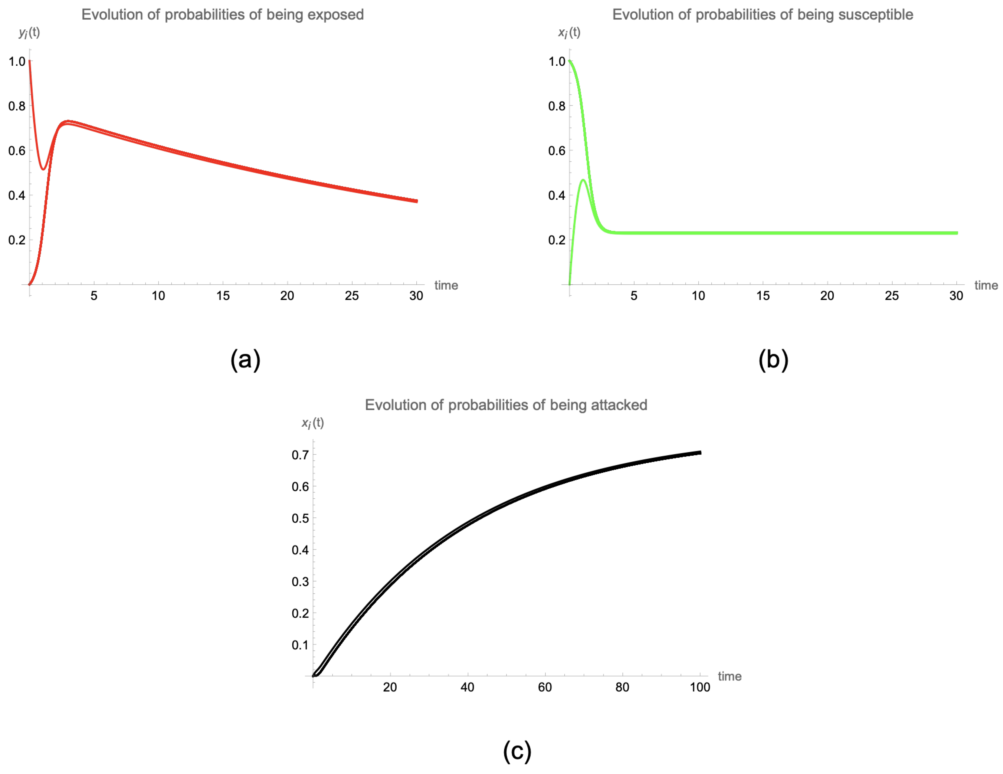
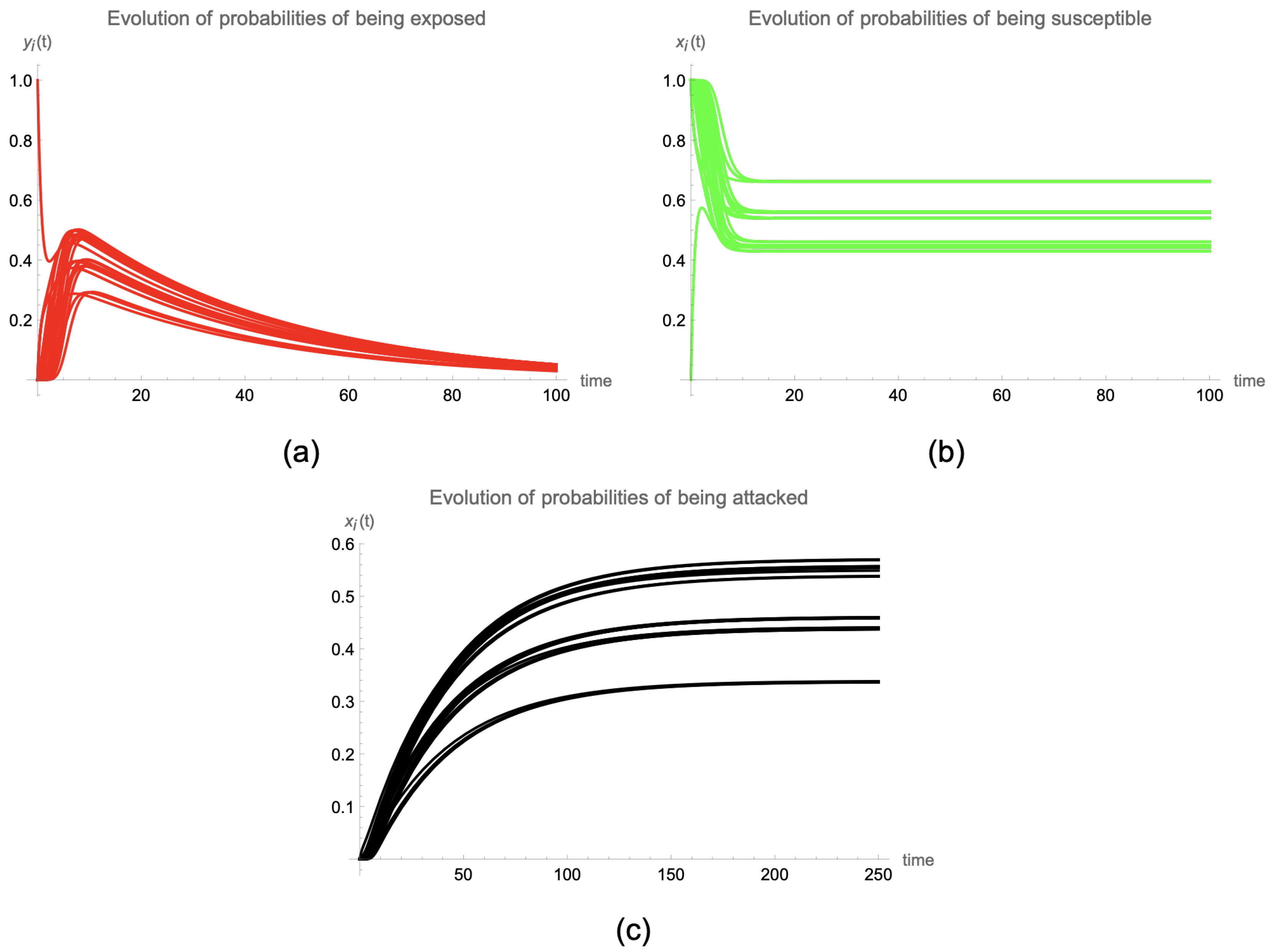
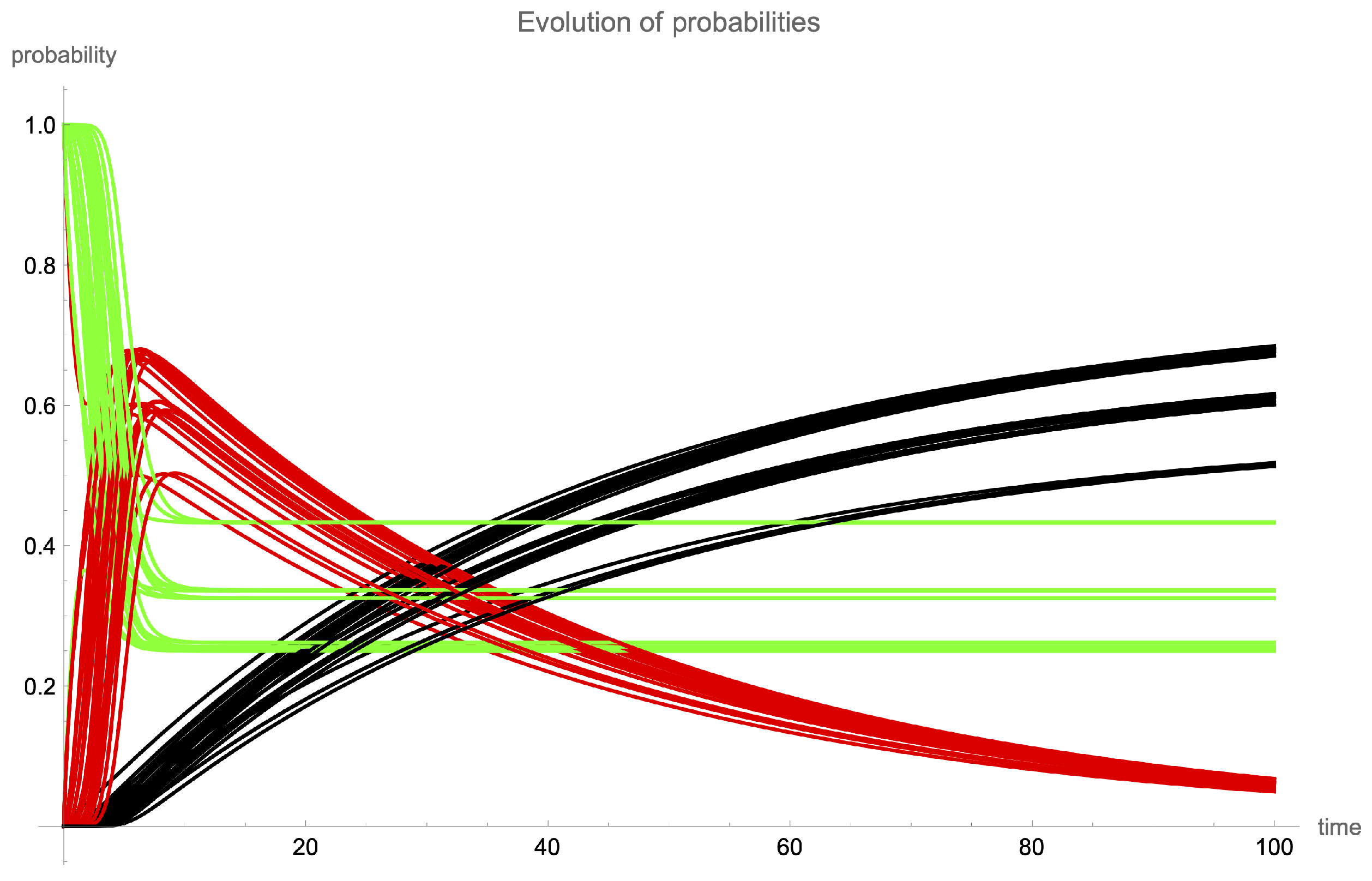
If the contact topology is described by means of a grid graph and, for the sake of simplicity (and visibility), only $n=6\times 6=36$ devices are deployed, then the evolution of probabilities is shown in Figure 7 when $c_{ij}=1,q_{ij}=0.5$ for $1\le i,j\le 36$, and ${\beta }_i=0.025,{\gamma }_i=0.5$, and the joint evolution of the different probabilities is presented in Figure 8. It can be seen how the population of devices are classified into several groups based on their evolution:

• In the case of the probability of being exposed, initially, three groups are formed that are characterized by the maximum value that $y_i\left(t\right)$ takes for $1\le i\le n$, although later they all converge to the same value of $y\left(\infty \right)$, the disease-free equilibrium point.
• In the case of the probability of being susceptible, it can be shown that from $t=0$, three groups of devices are created, depending on their positions within the complex network (degree and distance to the initially exposed node).
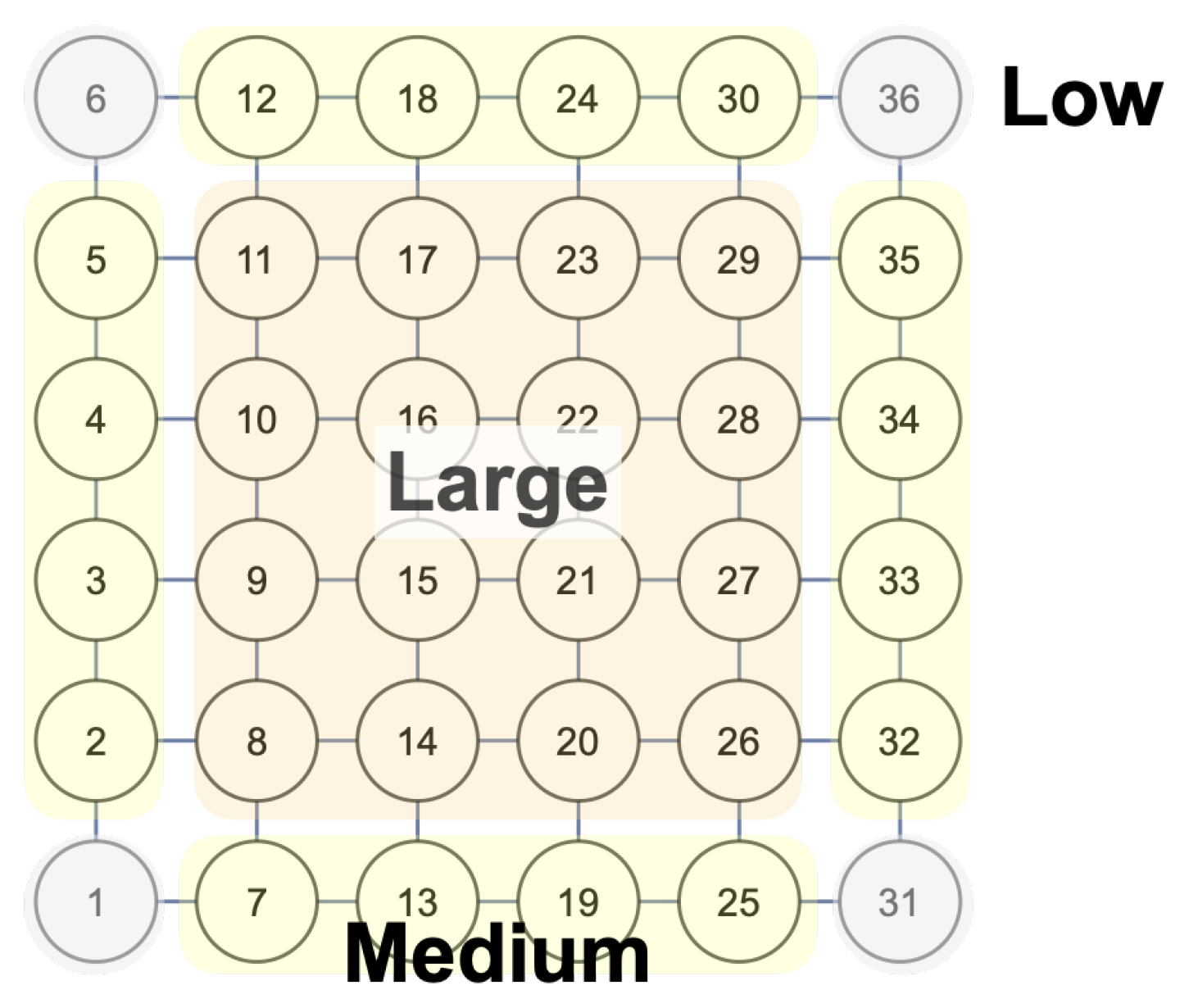
• As $x_i\left(t\right)+y_i\left(t\right)+z_i\left(t\right)=1$ for all $1\le i\le n$, the behavior of the probabilities of being attacked is similar to that of the probabilities of being susceptible, that is, three types of devices can be derived from the evolution considering the value of $z_i(\infty )$: $z_i(\infty )\approx 0.56$ (low values), $z_i(\infty )\in [0.66,0.67]$ (medium values), and $z_i(\infty )\in [0.73,0.74]$ (large values). The spatial distribution of these three types of nodes within the network is shown in Figure 9.

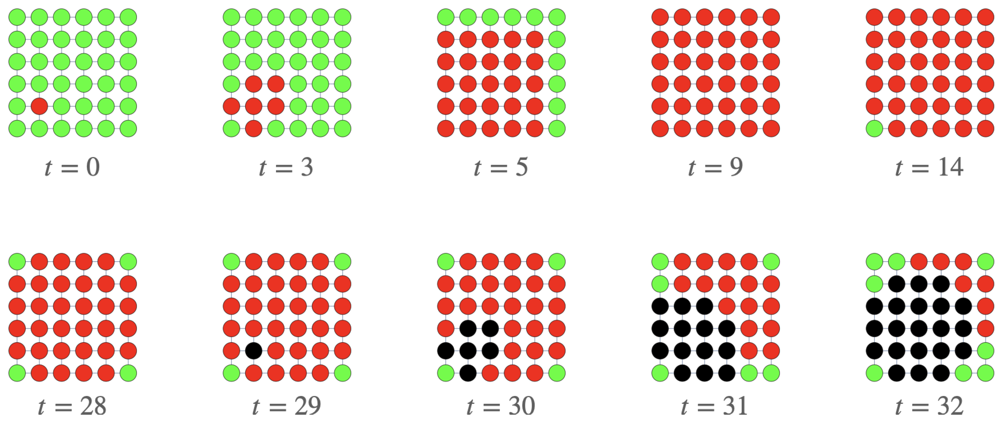
In Figure 10, the spatio-temporal spreading of the specimen of malicious code on the $6\times 6$ grid network is shown at different steps of time. In this simulation, the color of each node is assigned considering the greatest probability: $x_i\left(t\right),y_i\left(t\right)$ or $z_i\left(t\right)$ (that is, green, red and black for nodes whose highest probability is that of being susceptible, exposed and attacked, respectively).

3.3.2. Propagation on Heterogeneous Networks

Initially, suppose that all epidemiological coefficients are the same for all network devices, specifically: $c_{ij}=2,q_{ij}=0.25,\forall i,j$, and ${\beta }_i=0.01,{\gamma }_i=0.75,\forall i$. Moreover, assume that the IoT network is formed by $n=100$ nodes/devices, and its contact topology is determined by a random complex network defined by the Erdös–Rényi algorithm with probability p. Moreover, as in the previous simulations, it is assumed that at $t=0$, there is only one device with non-zero exposed probability: without loss of generality, we can suppose that it is the i-th device. Consequently, $y_i\left(0\right)>0$ and $y_j\left(0\right)=0$ for all $j\ne i$. 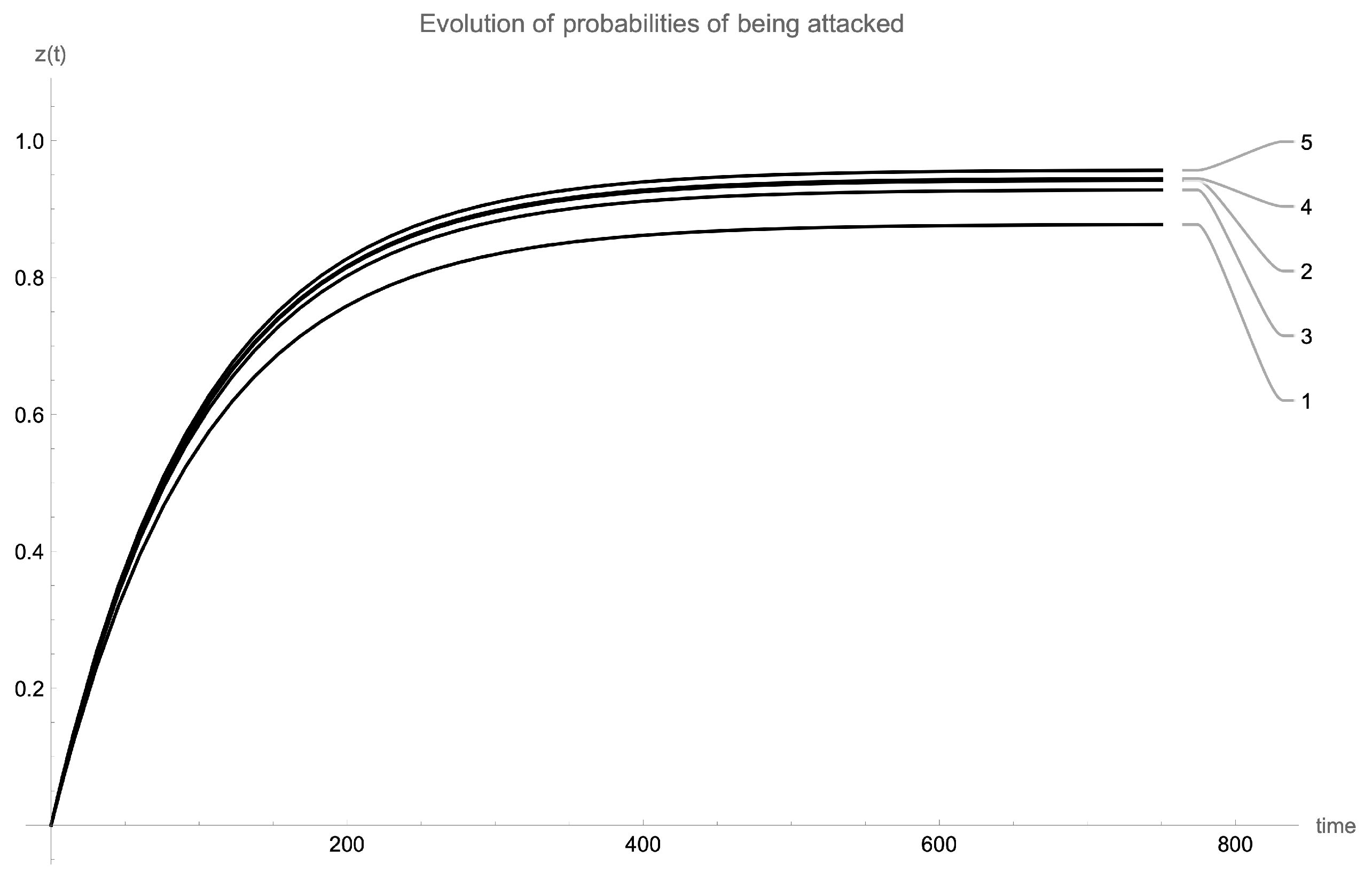In Figure 11, the evolution of the exposed probability $y_i\left(t\right)$ associated to the initially exposed device (the i-th device) is shown for each ER random network, where the link probability p takes the following values: $p=0,0.1,0.2,\dots ,0.9,1$. 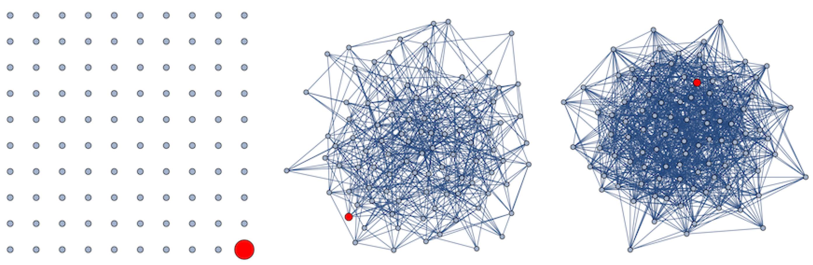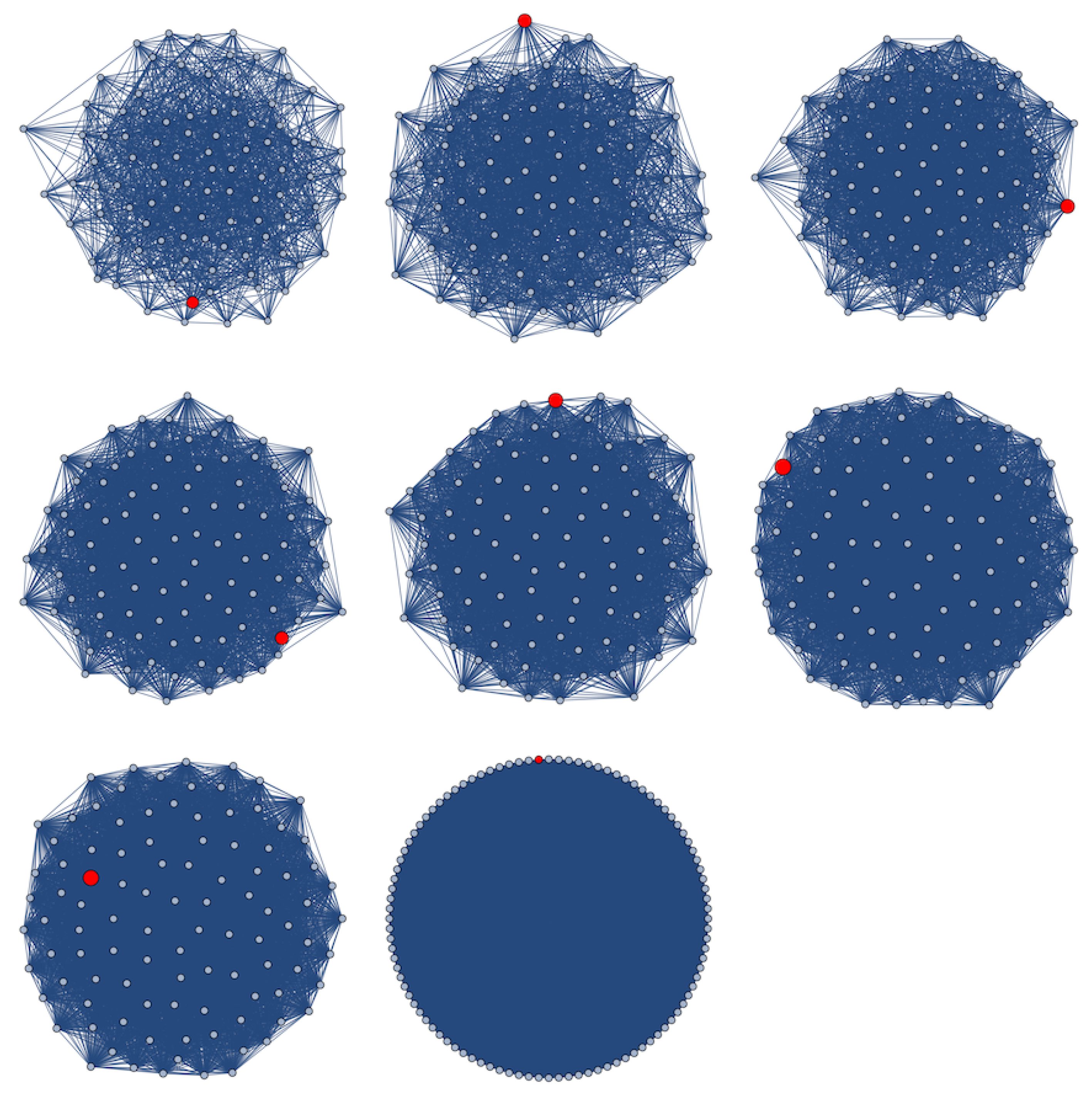In Figure 12, the explicit link structures of the ER random networks are shown (for $p=0$, the network consists of n isolated nodes, and for $p=1$, the complete graph is obtained), and in

Table 2. Structural characteristics of the ER random complex networks used in the simulations.

ER Network	Density	Diameter	Radius	Global Clustering	Mean Clustering	Mean Degree
$p=0$	0	∞	∞	0	0	0
$p=0.1$	0.097	4	3	0.092	0.0936	0.097
$p=0.2$	0.206	3	2	0.207	0.207	0.206
$p=0.3$	0.312	2	2	0.311	0.312	0.312
$p=0.4$	0.4	2	2	0.4	0.4	0.4
$p=0.5$	0.509	2	2	0.508	0.509	0.509
$p=0.6$	0.6036	2	2	0.602	0.602	0.603
$p=0.7$	0.705	2	2	0.705	0.705	0.705
$p=0.8$	0.804	2	2	0.804	0.804	0.804
$p=0.9$	0.899	2	2	0.899	0.899	0.899
$p=1$	1	1	1	1	1	1

, the global structural characteristics of these networks are shown. Note that as the link probability p increases, the higher the exposed probability values that are reached. The structural characteristics of the initially exposed devices are shown in

Table 3. Structural characteristics of the exposed devices at $t=0$ in the corresponding ER random complex network used in the simulations.

ER Network	Degree	Eccentricity	Closeness	Radial Index	Betweenness	Clustering
$p=0$	0	0	0	-	0	0
$p=0.1$	0.182	0.333	0.524	4.71	0.033	0.131
$p=0.2$	0.293	0.333	0.582	3.54	0.019	0.180
$p=0.3$	0.414	0.5	0.631	2.38	0.013	0.302
$p=0.4$	0.485	0.5	0.66	2.30	0.009	0.410
$p=0.5$	0.657	0.5	0.744	2.16	0.009	0.492
$p=0.6$	0.727	0.5	0.786	2.11	0.006	0.596
$p=0.7$	0.838	0.5	0.861	2.07	0.004	0.698
$p=0.8$	0.899	0.5	0.908	2.05	0.003	0.787
$p=0.9$	0.949	0.5	0.952	2.04	0.001	0.894
$p=1$	1	1	1	1.03	0	1

.

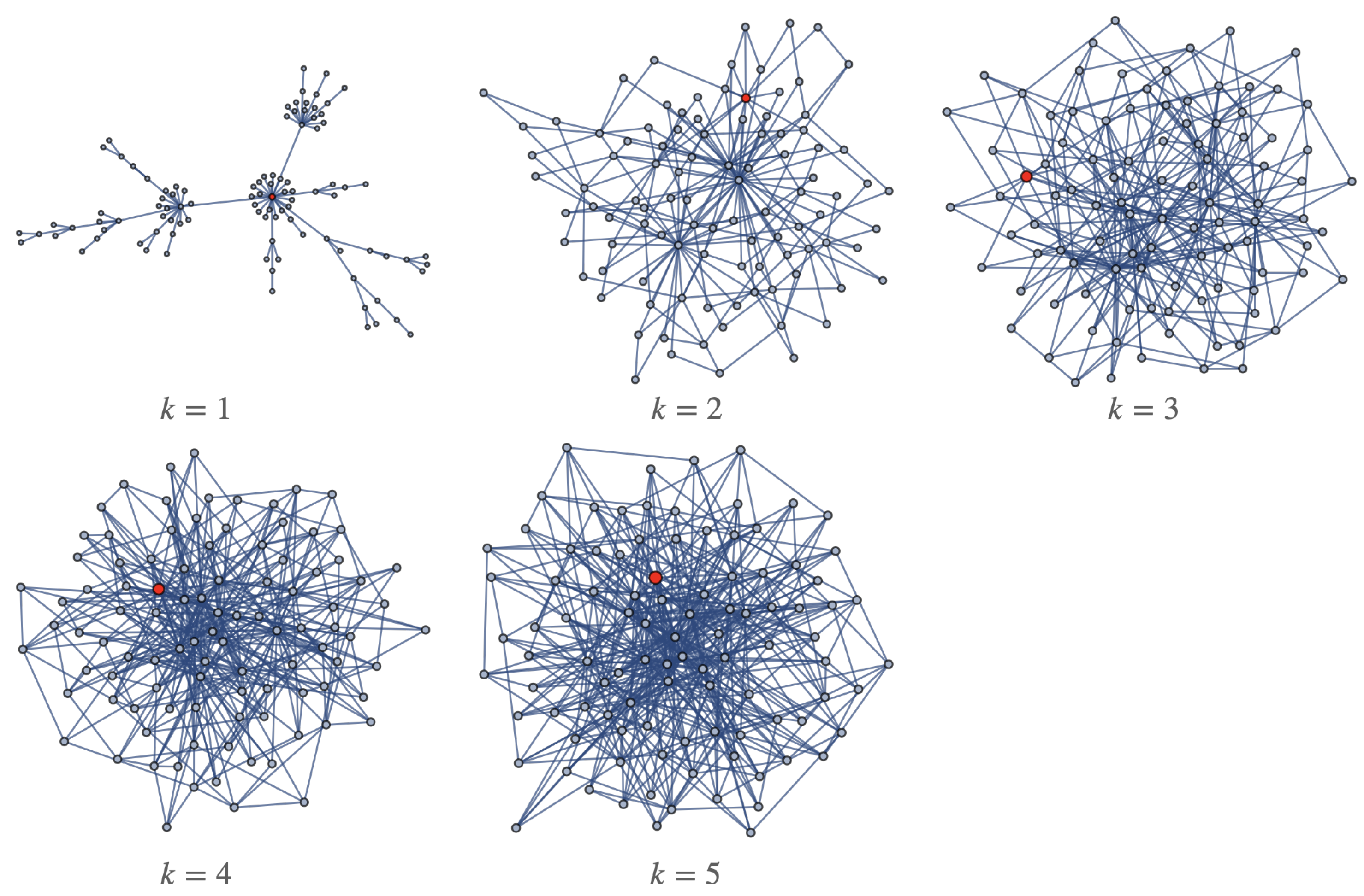
In Figure 13, the evolution of the attacked probabilities when the specimen of malicious code spreads on an IoT network that follows a scale-free topology where $k=1,2,3,4,5$ stand for the parameters of the Barabási–Albert algorithm (the explicit topologies of these networks are shown in Figure 14). The initial conditions and epidemiological coefficients employed are the same than those used in the last simulation. As is shown, the larger k is, the larger $z(\infty )$ is.

Finally, the behavior of spreading obviously depends on the structural characteristics of the initially exposed node. For example, in Figure 15 and Figure 16, the evolution of probabilities in each node of a scale-free network is shown, with $n=100,k=1$, $c_{ij}=1,q_{ij}=0.03$ for $1\le i,j\le 100$, and ${\beta }_i=0.01,{\gamma }_i=0.025$, for $1\le i\le 100$.

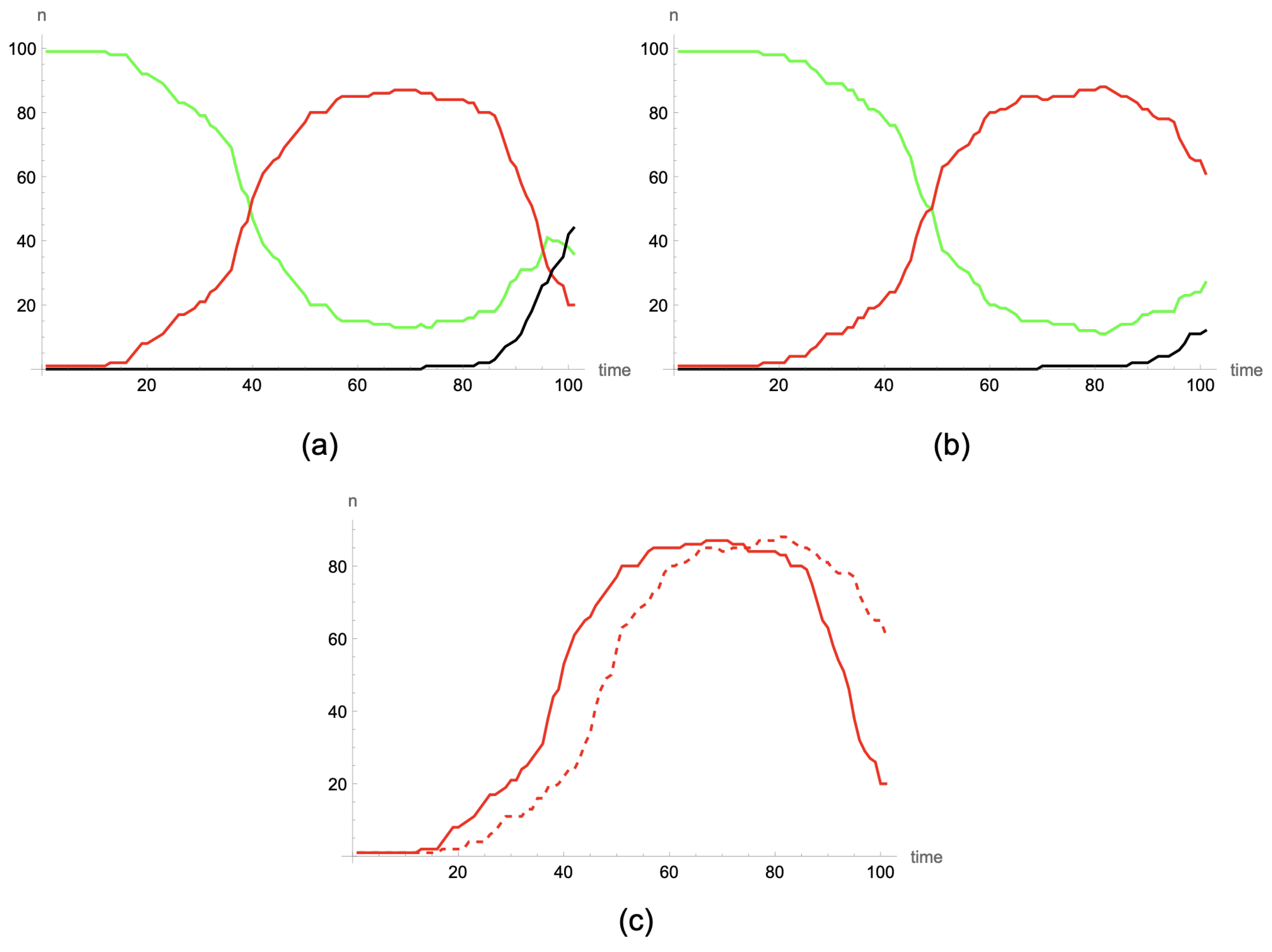
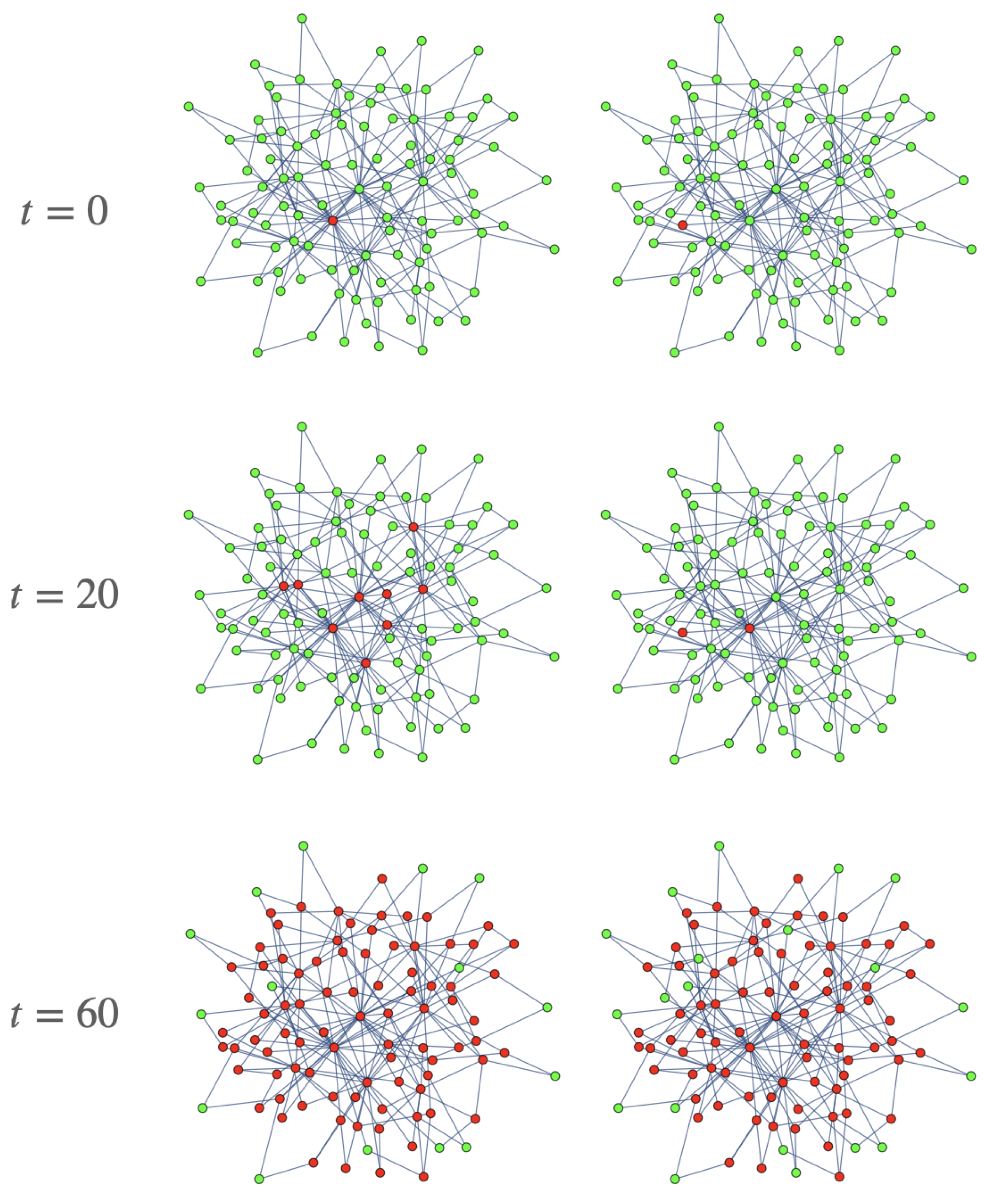
Specifically, in Figure 15a, the evolution of the number of devices with large probability of being susceptible (green), exposed (red) and attacked (black) when the “zero patient” is determined by the node with highest degree centrality is shown. The same simulation but considering as “patient zero” the node with the minimum degree centrality is presented in Figure 15b. Finally, in Figure 15c, the comparison between the simulations when the temporal evolution of the number of exposed devices is only represented is shown (the red dashed line stands for the case with the minimum degree centrality). In Figure 16, the spatial distribution of these nodes within the network is illustrated for three specific steps of time $t=0,t=20$, and $t=60$: the left column represents the evolution of the system when “patient zero” is the highest-degree node, whereas the right column stands for the evolution when “patient zero” is determined by the minimum degree centrality. Note that the growth of the number of devices with a higher probability of being exposed is faster in the first case (when the initially exposed node has the highest degree centrality) than in the second case, reaching its maximum earlier. However, in the end, both curves collapse to zero as the states of different nodes reach their equilibrium points.

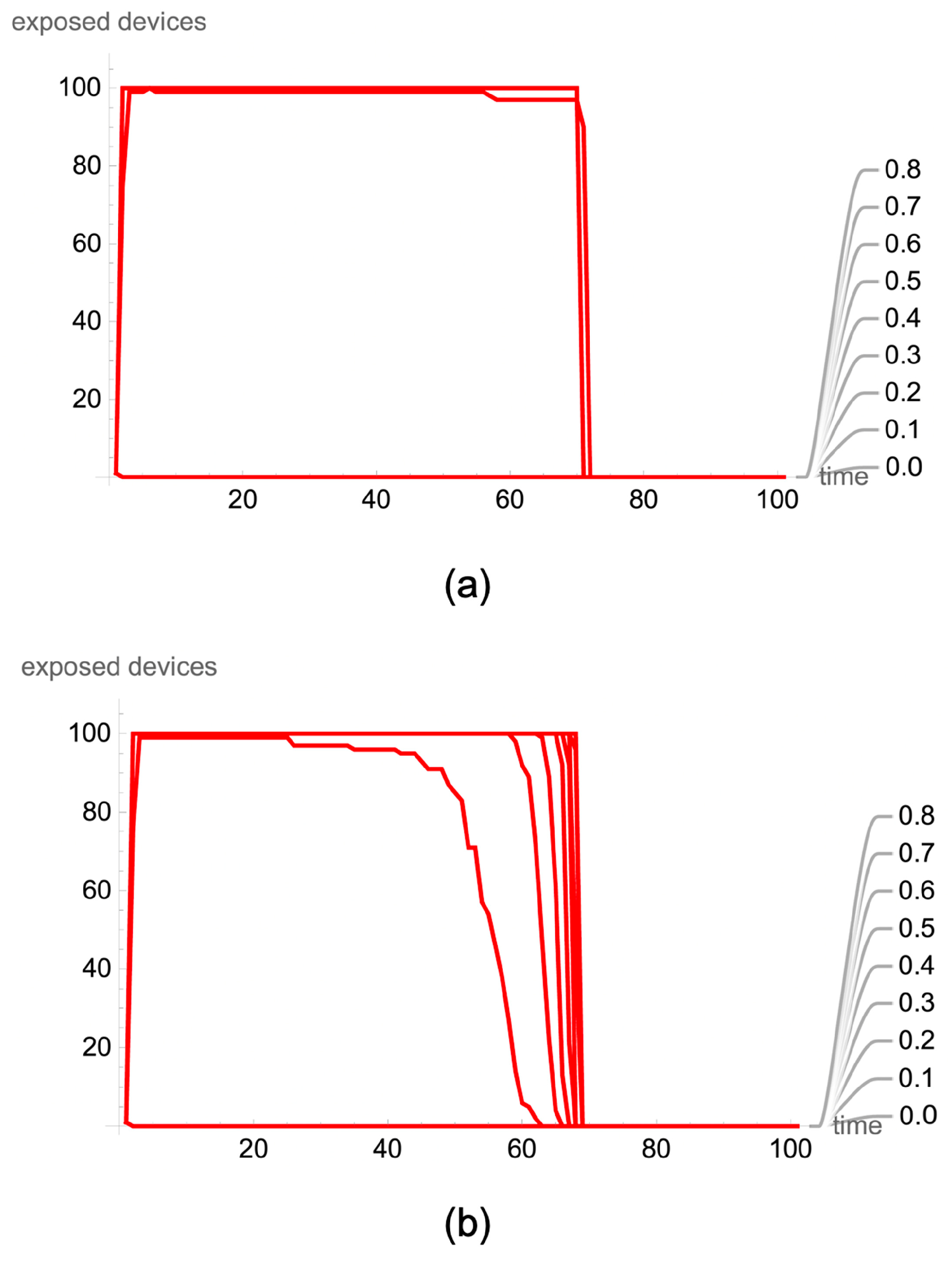
It seems reasonable to think that the topology of the network over which malware spreads conditions that propagation. It is expected that certain structural (and global) indices associated to the network (such as its density, average degree, average betweenness coefficient, etc.) serve as indicators of this process. In this sense, it can be observed that higher values of these indices cause the number of devices with a probability of being in the exposed state above a certain threshold to grow. For example, in Figure 17, some simulations are shown on ER random networks with $n=100$ devices, defined by different probabilities: $p=0,0.1,0.2,\dots ,0.9,1$. Additionally, for simplicity, the same epidemiological coefficients are assumed for all devices (${\beta }_i=0.01,{\gamma }_i=0.75,c_{ij}=2,q_{ij}=0.25$), and the node with the highest degree centrality is considered patient zero. Figure 17a shows the temporal evolution of the number of devices whose highest probability is to be exposed, while Figure 17b shows the evolution of the number of devices whose probability of being exposed is above $0.5$. It can be observed that as the reconnection probability p increases, the number of nodes with these characteristics also increases, peaking before eventually dropping to zero. Note (see

Table 4. Structural characteristics of the ER random complex networks used in the simulations.

p	Density	Diameter	Radius	Global Clustering	Mean Clustering	Average Degree	Average Eccentricity	Average Closeness	Average Betweenness
0	0.0	∞	∞	0.0	0.0	0.0	0.0	0.0	0.0
0.1	0.105	4	3	0.107	0.0979	0.105	0.314	0.457	0.0123
0.2	0.206	3	2	0.207	0.208	0.206	0.412	0.555	0.008
0.3	0.291	3	2	0.287	0.287	0.291	0.497	0.585	0.007
0.4	0.401	2	2	0.400	0.400	0.401	0.5	0.626	0.006
0.5	0.503	2	2	0.502	0.503	0.503	0.5	0.669	0.005
0.6	0.611	2	2	0.612	0.612	0.611	0.5	0.721	0.004
0.7	0.706	2	2	0.705	0.705	0.706	0.5	0.774	0.003
0.8	0.804	2	2	0.803	0.803	0.804	0.5	0.837	0.002
0.9	0.896	2	2	0.896	0.897	0.896	0.5	0.906	0.001
1	1.0	1	1	1.0	1.0	1.0	1.0	1.0	0.0

) that higher probability p corresponds to higher density, smaller diameter and radius, and more central values for different structural indices. Consequently, when the spread occurs on a network whose contact topology is defined by a complete graph, the malware propagates more “rapidly”.

4. Conclusions

In this work, a novel individual-based model for malware propagation on IoT networks is presented. One of the most important, and genuine, characteristics of the proposed model is the definition of the state of each node, which does not consist of its univocal determination at each step of time as is usual in the vast majority of models (susceptible device, exposed device, or attacked device), but rather is determined by a stochastic vector defined by the probabilities of being susceptible, exposed and attacked at this time. This is a deterministic model, where the local transition rules of the stochastic vector state of each device are described by means of a system of ordinary differential equations whose dependent variables represent the last three mentioned variables.

It is shown that the probability vector evolves to a steady state with $y_i(\infty )=0$ for $1\le i\le n$ such that the values of the other two probabilities (the probability of remaining susceptible $s_i(\infty )$ and the probability of being attacked $z_i(\infty )=1-x_i(\infty )$) and the maximum value taken by the probability of being exposed $y_i\left(t\right)$ depend on the structural properties of the corresponding node within the complex network and the global structural characteristics of the complex network that describes the contact/communication topology of the IoT network.

The determination of security countermeasures is an important issue [26,27]. From the analysis of the model, and more specifically from the analysis of the basic reproductive number ${\mathcal{R}}_0$, it is possible to obtain control strategies for the epidemic process (consisting of reducing the number of devices capable of transmitting the malware). Thus, the objective would be to reduce this threshold parameter to below 1. Taking into account the explicit expression of $R_0$, this could be achieved by decreasing w or increasing both the recovery rate and the attack rate. Realistically, in this case, it would only be possible to decrease the number of contacts or increase the recovery rate.

In my opinion, such models that predict the spread of a particular specimen of malware in an IoT network, while they have not received as much attention as models for detecting the presence of malware, can offer solutions of the same level of importance. In this sense, I believe that their implementation in the security operation centers (SOCs) is particularly interesting and useful such that after the successful detection of malware, real-time predictions about the future evolution of malware (considering different types of initial conditions) could be given.

Future work will focus on carrying on a more in-depth theoretical study of the explicit expression of the “disease-free” steady state reached by the system that takes into account the particular characteristics of each node/device. It is also of great interest to study in depth the design of different metrics that allow to correctly analyze how fast a specific malware specimen spreads when the state of the devices is probabilistic.