The Grad–Shafranov Equation in Cap-Cyclide Coordinates: The Heun Function Solution

Abstract

The Grad–Shafranov plasma equilibrium equation was originally solved analytically in toroidal geometry, which fitted the geometric shape of the first Tokamaks. The poloidal surface of the Tokamak has evolved over the years from a circular to a D-shaped ellipse. The natural geometry that describes such a shape is the prolate elliptical one, i.e., the cap-cyclide coordinate system. When written in this geometry, the Grad–Shafranov equation can be solved in terms of the general Heun function. In this paper, we obtain the complete analytical solution of the Grad–Shafranov equation in terms of the general Heun functions and compare the result with the limiting case of the standard toroidal geometry written in terms of the Fock functions.

1. Introduction

The simple equation $\nabla P=J\times B$ for plasma equilibrium, where $P$ is the kinetic plasma pressure, $J$ is the plasma current density, and $B$ is the magnetic field, is among the most robust magneto-hydrodynamic equations in plasma physics, and its applicability extends from laboratory plasmas to astrophysical plasmas. Introducing the flux function over a poloidal surface $S_{\mathrm{pol}}$:

$$\psi =\frac{1}{2\pi }{\displaystyle \underset{S\mathrm{pol}}{\iint }B·ds},$$

(1)

assuming axial symmetry and using cylindrical coordinates $R,Z,\phi$, this equilibrium equation can be written as a non-linear second-order partial differential equation:

$$\frac{{\partial }^2\psi }{\partial R^2}-\frac{1}{R}\frac{\partial \psi }{\partial R}+\frac{{\partial }^2\psi }{\partial Z^2}={\mu }_{0}R{J}_{\phi },$$

(2)

where $J_{\phi }$ is the axisymmetric current density. This equation is referred to as the Grad–Shafranov equation and its analytical solution based on toroidal geometry [1,2,3] underlies the present Tokamak experiments. It should be noted that in vacuum ($J_{\phi }=0$), this equation is similar (but with a minus sign in front of the first-derivative term) to the scalar Laplace equation; in fact, this equation always coincides in vacuum with the Laplace equation for the toroidal component of the vector potential [4].

The first Tokamaks had a circular cross section, so the toroidal geometry was the natural one for solving Equation (2). However, over the years, for several technical and physical reasons, the Tokamak section evolved into a deformed elongated elliptical shape (D-shape). In the second half of the 19th century, the analytical solution of the related Laplace equation in several different geometries was studied in depth [5,6,7] in order to also find an analytical solution for oblate and prolate toroidal geometries. The book by Spencer and Moon [8] suggests a good overview of all this work performed up to that time. An analytical solution for torus inductance was obtained by Fock [9] and the first analytical solution of the Laplace equation in elliptic oblate coordinates was found by Lebedev [10]. Eventually, a team of Japanese scientists found the analytical solution of the vacuum Grad–Shafranov equation for an oblate toroidal system [11,12]. This solution, as well as the solution for the analogous Laplace equation [8], was written in terms of the so-called Wangerin functions, but the explicit evaluation of these functions has never been proposed. Further, the oblate geometry is even worse than the standard toroidal geometry for working with the modern elliptical elongated Tokamaks.

Recently, Crisanti [13] came to the solution of the Grad–Shafranov equation in the case of the elliptic prolate geometry, writing Equation (1) in the cap-cyclide coordinates; but in this case, too, the solution was written in terms of the Wangerin functions and hence its actual representation was not illustrated and/or suggested. Eventually, it was found [14] that the three-dimensional Laplace equation can be transformed into the general Heun equation [15,16] by an appropriate coordinate transformation. Further, for some particular cases of the parameters, the solution can be expressed as a linear combination of the generalized [17,18] or ordinary [18,19,20] hypergeometric functions. As mentioned above, the Laplace equation and the Grad–Shafranov equation when written in standard cylindrical coordinates differ from each other only in the sign of the first-derivative term. In the present paper, restricting ourselves to the two-dimensional case, the Grad–Shafranov problem is generalized to a family of equations by introducing an appropriate parameter. This made it possible to write down the solution of the Laplace and Grad–Shafranov equations in a unified way in terms of the general Heun functions and to compare the obtained results with the limiting case of the solution for standard toroidal coordinates. As explained in [13,21], the analytical solution, expressed in the geometry that best suits the problem under consideration, opens up the possibility of writing a plasma inverse equilibrium code, which, based on magnetic measurements external to the plasma, is capable of recovering some important plasma characteristics such as current density profile and volume-integrated kinetic pressure.

2. Cap-Cyclide Coordinates

The cap-cyclide coordinates offer a natural framework for studying problems with elliptical prolate boundary conditions. In the complex plane, the coordinate transformation is given via the equation

$$\frac{k^{1/4}}{2ai}·\frac{1+i{k}^{1/4}sn\left(w\right)}{1-i{k}^{1/4}sn\left(w\right)}=R\left(\mu ,\nu \right)+iZ\left(\mu ,\nu \right),w\left(\mu ,\nu \right)=\mu +i\nu ,$$

(3)

where $sn$ is the Jacobi elliptic sine function and a is a scaling constant. The functions $R\left(\mu ,\nu \right)$ and $Z\left(\mu ,\nu \right)$ satisfy the Cauchy–Riemann conditions

$$\frac{\partial R}{\partial \mu }=\frac{\partial Z}{\partial \nu } ,\frac{\partial R}{\partial \nu }=-\frac{\partial Z}{\partial \mu }.$$

(4)

For the real-space coordinates $X,Y,Z$, the coordinate transformations are given as

$$X=\frac{\mathsf{\Lambda }}{a\mathsf{\Gamma }}sn\left(\mu ,k\right)dn\left(\nu ,k_1\right)\cos \phi ,$$

(5)

$$Y=\frac{\mathsf{\Lambda }}{a\mathsf{\Gamma }}sn\left(\mu ,k\right)dn\left(\nu ,k_1\right)\sin \phi ,$$

(6)

and

$$Z=\frac{k^{1/4}\mathsf{\Pi }}{2a\mathsf{\Gamma }}.$$

(7)

Here, $a$ defines the center of the coordinate system, $k$ and $k_1$ are, respectively, the parameter and the complementary parameter of the elliptical integrals: $k+k_1=1$, and

$$\mathsf{\Lambda }=1-d{n}^2\left(\mu ,k\right)s{n}^2\left(\nu ,k_1\right),$$

(8)

$$\mathsf{\Gamma }=s{n}^2\left(\mu ,k\right)d{n}^2\left(\nu ,k_1\right)+{\left(\mathsf{\Lambda }/k^{1/4}+cn\left(\mu ,k\right)dn\left(\mu ,k\right)sn\left(\nu ,k_1\right)cn\left(\nu ,k_1\right)\right)}^2,$$

(9)

$$\mathsf{\Pi }=\left({\mathsf{\Lambda }}^2/k^{1/2}\right)-\left(s{n}^2\left(\mu ,k\right)d{n}^2\left(\nu ,k_1\right)+c{n}^2\left(\mu ,k\right)d{n}^2\left(\mu ,k\right)s{n}^2\left(\nu ,k_1\right)c{n}^2\left(\nu ,k_1\right)\right).$$

(10)

The coordinate transformation (5)–(10) can generate a wide range of distinct geometries by adjusting the parameter $k$. When $\mu$ approaches 0, the geometric shape given by the parametric curve $\{x(\nu ),y(\nu )\}$ at constant $\mu$ and $k$ tends to the bipolar (standard toroidal) form, regardless of $k$ (Figure 1).

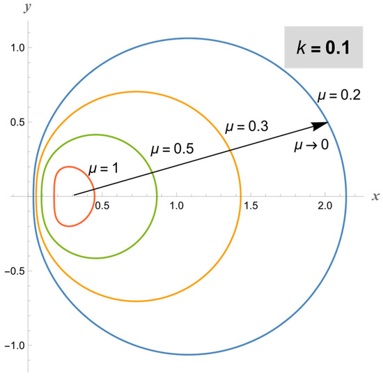
Figure 1. For $\mu \to 0$, the constant-$\mu ,k$ cross-section $\{x(\nu ),y(\nu )\}$ tends to a standard bipolar shape regardless of $k$.

However, for any fixed non-zero $\mu$, the shape depends on the value of $k$. When $k$ approaches 0, the surfaces tend to adopt a bean-like shape. For intermediate values of $k$, the surfaces can either be D shaped or purely elliptical prolate, similar to the geometry encountered in most current tokamak experiments. Finally, as $k$ approaches 1, all surfaces resemble standard toroidal ones, irrespective of μ (Figure 2).

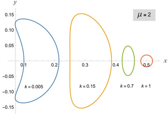
Figure 2. For $k\to 0$, the surfaces are bean shaped; for intermediate k, the surfaces can be either D or elliptical prolate; for $k\to 1$, the surfaces tend to be standard bipolar shaped.

3. The Generalized Laplace Equation

As mentioned above, in vacuum, the Laplace equation and the Grad–Shafranov equation in cylindrical coordinates differ only in the sign of the first derivative, and we have the following two equations:

$$\frac{{\partial }^2\psi }{\partial R^2}\pm \frac{1}{R}\frac{\partial \psi }{\partial R}+\frac{{\partial }^2\psi }{\partial Z^2}=0.$$

(11)

To treat both equations in the same way, we consider the auxiliary equation

$$\frac{{\partial }^{2}w}{\partial R^2}+\frac{{\partial }^{2}w}{\partial Z^2}+\frac{A}{R^2}=0$$

(12)

with a variable parameter $A$, to which the two equations are reduced by the transformation

$$\psi =R^{-{\sigma }_0/2}w$$

(13)

(${\sigma }_0=+1$ for the AC-Laplace equation and ${\sigma }_0=-1$ or ${\sigma }_0=3$ for the Grad–Shafranov equation). For the Laplace and Grad–Shafranov equations, the parameter $A$ takes the values $A=1/4$ and $A=-3/4$, respectively; however, we will treat the problem for arbitrary A. Correspondingly, Equation (11) is now generalized to the equation

$$\frac{{\partial }^2\psi }{\partial R^2}+\frac{{\sigma }_0}{R}\frac{\partial \psi }{\partial R}+\frac{{\partial }^2\psi }{\partial Z^2}=0,$$

(14)

which serves as the starting point for this study. Note that transformation (13) reduces this equation to Equation (12) with

$$A=\frac{{\sigma }_0}{2}\left(1-\frac{{\sigma }_0}{2}\right)$$

(15)

The form of Equation (12) is advantageous in that in changing the coordinate system, only the two derivative terms are transformed. The sum of these terms can be conventionally considered as the Cartesian Laplacian of the function $w$ with respect to coordinates $R,Z$. Note that the Laplacian

$$\mathsf{\Delta }w\left(R,Z\right)=\frac{{\partial }^{2}w}{\partial R^2}+\frac{{\partial }^{2}w}{\partial Z^2}$$

(16)

in a general two-dimensional curvilinear coordinate system $(q_1,q_2)$ such that

$$R={\phi }_1\left(q_1,q_2\right),Z={\phi }_2\left(q_1,q_2\right),$$

(17)

is written as

$$\mathsf{\Delta }w\left(q_1,q_2\right)=\frac{1}{H_1{H}_2}\left[\frac{\partial }{\partial q_1}\left(\frac{H_2}{H_1}\frac{\partial w}{\partial q_1}\right)+\frac{\partial }{\partial q_2}\left(\frac{H_1}{H_2}\frac{\partial w}{\partial q_2}\right)\right],$$

(18)

where

$$H_i=\sqrt{{\left(\frac{\partial {\phi }_1}{\partial q_1}\right)}^2+{\left(\frac{\partial {\phi }_2}{\partial q_2}\right)}^2},i=1,2,$$

(19)

are the scale factors (Lamé coefficients).

4. Solution in Bipolar Coordinates

For reference purposes, we reproduce here the solution of the generalized Laplace Equation (14) in bipolar coordinates. Having in mind a two-dimensional version of the three-dimensional standard toroidal coordinates, consider the 2D bipolar coordinates $r,\theta$ defined by the equations

$$(x,y)=\left(\frac{a\sinh r}{\cosh r-\cos \theta },\frac{a\sin \theta }{\cosh r-\cos \theta }\right),$$

(20)

where $x,y$ are real-space Cartesian coordinates and a is a scaling constant. In the coordinates $r,\theta$, the 2D Cartesian Laplacian

$${\mathsf{\Delta }}_{C}w=\frac{{\partial }^{2}w}{\partial x^2}+\frac{{\partial }^{2}w}{\partial y^2}$$

(21)

becomes

$${\mathsf{\Delta }}_{B}w=\frac{{\left(\cosh r-\cos \theta \right)}^2}{a^2}\left(\frac{{\partial }^{2}w}{\partial r^2}+\frac{{\partial }^{2}w}{\partial {\theta }^2}\right).$$

(22)

With this, by putting $(R,Z)=(x,y)$, Equation (12) is rewritten as

$$\frac{{\partial }^{2}w}{\partial r^2}+\frac{{\partial }^{2}w}{\partial {\theta }^2}+\frac{Aw}{{\sinh }^{2}r}=0.$$

(23)

Separation of variables in the form

$$w=u(r)\mathsf{\Theta }(\theta )$$

(24)

and a separation constant $p$ yields

$$\mathsf{\Theta }=\sin (p\theta +{\theta }_0),$$

(25)

where ${\theta }_0$ is an arbitrary constant. The equation for the radial component $u(r)$ then reads

$$\frac{d^{2}u}{d{r}^2}+\left(\frac{A}{{\sinh }^{2}r}-p^2\right)u=0.$$

(26)

By the change in the variables

$$u=\sqrt{\sinh r}v\left(s(r)\right),s(r)=\cosh r$$

(27)

this equation is reduced to the Legendre equation for $v(s)$ [22]. As a result, we obtain the general solution

$$u(r)=\sqrt{\sinh r}\left(C_1{P}_{p-1/2}^q\left(\cosh r\right)+C_2{Q}_{p-1/2}^q\left(\cosh r\right)\right),q=\sqrt{\frac{1}{4}-A},$$

(28)

where $C_1$ and $C_2$ are arbitrary constants, and $P_{p-1/2}^q$ and $Q_{p-1/2}^q$ are the Legendre functions of the first and second kind, respectively. We note that for the AC-Laplace equation, the parameter $q$ is zero, while for the Grad–Shafranov equation, $q=1$.

5. Solution in Cap-Cyclide Coordinates

It can be shown that the Laplacian in cap-cyclide coordinates is written as

$${\mathsf{\Delta }}_{CC}w=\frac{a^2{\mathsf{\Gamma }}^2}{{\mathsf{\Lambda }}^2{\mathsf{\Omega }}^2}\left(\frac{{\partial }^{2}w}{\partial {\mu }^2}+\frac{{\partial }^{2}w}{\partial {\nu }^2}\right),$$

(29)

where

$$\mathsf{\Omega }=\sqrt{\left(1-sn{\left(\mu ,k\right)}^{2}dn{\left(\nu ,k_1\right)}^2\right)\left(dn{\left(\nu ,k_1\right)}^2-ksn{\left(\mu ,k\right)}^2\right)}.$$

(30)

With this, Equation (12) is checked to be rewritten as

$$\frac{{\partial }^{2}w}{\partial {\mu }^2}+\frac{{\partial }^{2}w}{\partial {\nu }^2}+A\left(\frac{1}{sn{\left(\mu ,k\right)}^2}+ksn{\left(\mu ,k\right)}^2\right)-A\left(\frac{k}{dn{\left(\nu ,k_1\right)}^2}+dn{\left(\nu ,k_1\right)}^2\right)=0.$$

(31)

It is readily seen that this is a separable equation. Then, by putting

$$w\left(\mu ,\nu \right)=U\left(\mu \right)V\left(\nu \right),$$

(32)

we have the ordinary differential equations

$$U^{″}\left(\mu \right)+A\left(\frac{1}{sn{\left(\mu ,k\right)}^2}+ksn{\left(\mu ,k\right)}^2+B\right)U\left(\mu \right)=0,$$

(33)

$$V^{″}\left(\nu \right)-A\left(\frac{k}{dn{\left(\nu ,k_1\right)}^2}+dn{\left(\nu ,k_1\right)}^2+B\right)V\left(\nu \right)=0,$$

(34)

where $B$ is the separation constant.

Now, applying the variable change

$$U=z^{\sigma }y(z),z=sn{\left(\mu ,k\right)}^2,$$

(35)

$$\sigma =\frac{1}{4}\left(1\pm \sqrt{1-4A}\right)=\frac{{\sigma }_0}{4}$$

(36)

(we recall that ${\sigma }_0$ is the parameter of the starting Equation (14)), Equation (33) is reduced to the general Heun equation [15,16]

$$y^{″}+\left(\frac{\gamma }{z}+\frac{\delta }{z-1}+\frac{\epsilon }{z-a}\right)y^{\prime }+\frac{\alpha \beta z-q}{z\left(z-1\right)\left(z-a\right)}y=0$$

(37)

with parameters

$$(\gamma ,\delta ,\epsilon ,\alpha ,\beta )=\left(\frac{1+4\sigma }{2},\frac{1}{2},\frac{1}{2},2\sigma ,\frac{1}{2}\right),$$

(38)

and

$$a=\frac{1}{k},q=\frac{2\left(1+k\right)\sigma -A\left(B+k+1\right)}{4k}.$$

(39)

Similarly, the transformation

$$V=z^{\sigma }y(z),z=dn{\left(\nu ,k_1\right)}^2$$

(40)

with the same parameter $\sigma$, as given by Equation (36), reduces Equation (34) to the general Heun equation with all the same parameters except the location $a$ of the third finite singularity of the general Heun equation and the accessory parameter $q$. This time

$$a_1=k,q_1=\frac{2\left(1+k\right)\sigma -A\left(B+k+1\right)}{4}.$$

(41)

With this, a fundamental solution of Equation (12) given by Equation (32) is finally written as

$$\begin{array}{c}w=sn{\left(\mu ,k\right)}^{2\sigma }dn{\left(\nu ,k_1\right)}^{2\sigma }\times \\ \mathrm{HeunG}\left(1/k,q;\alpha ,\beta ,\gamma ,\delta ;sn{\left(\mu ,k\right)}^2\right)\mathrm{HeunG}\left(k,q_1;\alpha ,\beta ,\gamma ,\delta ;d{n}^2\left(\nu ,k_1\right)\right).\end{array}$$

(42)

This is a particular solution of Equation (31). To construct the general solution, the Heun functions included in this solution should be replaced by general solutions of the general Heun Equation (37) for the radial and angular cases.

We conclude this section by noting that the derived solution is valid for arbitrary constant ${\sigma }_0$ (or, equivalently, constant $A$), which is just the parameter that defines the difference between the Laplace and Grad–Shafranov equations.

6. Bipolar Limit of Cap-Cyclide Coordinates for the Grad–Shafranov Equation

It is easy to check that the cap-cyclide coordinates (5)–(7) are transformed into bipolar (toroidal) coordinates (20) if $k=1$, $r=2\mu$ and $\theta =2\nu +\pi /2$. It can be further verified that Equation (33) for the radial part then becomes Equation (26) by setting

$$B=-2-4p^2/A.$$

(43)

Consider the toroidal limit of cap-cyclide coordinates for the Grad–Shafranov equation for which $A=-3/4$ so that $B=-2+16p^2/3$.

6.1. Radial Solution

The radial part of the general solution of Equation (33) is written as the linear combination

$$U=C_1{U}_1+C_2{U}_2,$$

(44)

where $C_{1,2}$ are arbitrary constants, and $U_1$ and $U_2$ present a pair of independent fundamental solutions of Equation (33). Since the last equation reduces to the general Heun Equation (37), these fundamental solutions are represented as

$$U_{1,2}=z^{3/4}\left(c_1{u}_1+c_2{u}_2\right),$$

(45)

where $c_{1,2}$ are arbitrary constants; and in the limit $k=1$,

$$u_1=\mathrm{HeunG}\left(1,\frac{3}{4}+p^2;\frac{1}{2},\frac{3}{2},2,\frac{1}{2};z\right),$$

(46)

$$u_2=\mathrm{HeunG}\left(0,-p^2;\frac{1}{2},\frac{3}{2},\frac{1}{2},2;1-z\right)$$

(47)

with

$$z={\tanh }^2\left(\mu \right).$$

(48)

Consider the function $u_1$. Since $a=1$ here, the general Heun function reduces to the ordinary hypergeometric function [15]:

$$u_1=\mathrm{HeunG}\left(1,\frac{3}{4}+p^2;\frac{1}{2},\frac{3}{2},2,\frac{1}{2};z\right)={\left(1-z\right)}^p{}_{2}F{}_1\left(\frac{1}{2}+p,\frac{3}{2}+p;2;z\right).$$

(49)

With this, setting $c_1=1,c_2=0$ in Equation (44), we construct the fundamental solution

$$U_1={\mathrm{sech}}^{2p}\left(\mu \right){\tanh }^{3/2}\left(\mu \right){}_2{F}_1\left(p+\frac{1}{2},p+\frac{3}{2};2;{\tanh }^2\left(\mu \right)\right).$$

(50)

Using the following representation of the hypergeometric function in terms of the Legendre $P$ function [22]:

$${}_2{F}_1\left(b,b+1;2;y\right)=\frac{i{\left(1-y\right)}^{-b}}{b\left(b-1\right)\sqrt{y}}{P}_{b-1}^1\left(\frac{1+y}{1-y}\right),0<y<1,$$

(51)

this solution is rewritten as

$$U_1=\frac{2i\sqrt{2}}{4p^2-1}\sqrt{\sinh \left(2\mu \right)}{P}_{p-1/2}^1\left(\cosh \left(2\mu \right)\right),$$

(52)

which, since $2\mu =r$, exactly reproduces the first independent solution of (28) with $A=-3/4$.

To construct the second fundamental solution, consider the function $u_2$. Since $a=0$ here, the general Heun function involved again reduces to the ordinary hypergeometric function ($z={\tanh }^2\left(\mu \right)$):

$$u_2=\mathrm{HeunG}\left(0,-p^2;\frac{1}{2},\frac{3}{2},\frac{1}{2},2;1-z\right)={\left(1-z\right)}^p{}_{2}F{}_1\left(\frac{1}{2}+p,\frac{3}{2}+p;1+2p;1-z\right).$$

(53)

Then, the second fundamental solution should have the form

$$U_2={\mathrm{sech}}^{2p}\left(\mu \right)z^{3/4}\left(c_1·{}_2{F}_1\left(p+\frac{1}{2},p+\frac{3}{2};2;z\right)+c_2·{}_2{F}_1\left(p+\frac{1}{2},p+\frac{3}{2};2p+1;1-z\right)\right).$$

(54)

It turns out that it is convenient to choose

$$c_1=\frac{-i\pi }{2},c_2=-\frac{\mathsf{\Gamma }\left(p-1/2\right)\mathsf{\Gamma }\left(p+1/2\right)}{2\mathsf{\Gamma }\left(2p+1\right)},$$

(55)

since then, using the following representation of the Legendre $Q$ function [22]:

$$c_1{}_{2}F{}_1\left(p+\frac{1}{2},p+\frac{3}{2};2;y\right)+c_2{}_{2}F{}_1\left(p+\frac{1}{2},p+\frac{3}{2};2p+1;1-y\right)=\frac{i{\left(1-y\right)}^{-p-\frac{1}{2}}{Q}_{p-\frac{1}{2}}^1\left(\frac{y+1}{1-y}\right)}{\left(p-\frac{1}{2}\right)\left(p+\frac{1}{2}\right)\sqrt{y}},$$

(56)

the second fundamental solution can be written as

$$U_2=\frac{2i\sqrt{2}}{4p^2-1}\sqrt{\sinh \left(2\mu \right)}{Q}_{p-1/2}^1\left(\cosh \left(2\mu \right)\right),$$

(57)

which, with $2\mu =r$, reproduces the second independent solution of (28).

6.2. Angular Solution

The general solution of the Grad–Shafranov equation for the angular part, i.e., the general solution of Equation (34), is written as

$$V=C_3{V}_1+C_4{V}_2,$$

(58)

$$V_{1,2}=z^{3/4}\left(c_1{v}_1+c_2{v}_2\right),$$

(59)

where $C_{1,2}$, $c_{1,2}$ are arbitrary constants and $v_{1,2}$ are two independent fundamental solutions of the general Heun Equation (37) with parameters given by Equations (38) and (41). Note that in the limit $k\to 1$ the parameters become identical to those of the general Heun equation for the radial part. The only difference is the transformation of the independent variable, which is now given as

$$z=dn{\left(\nu ,k_1\right)}^2.$$

(60)

Interestingly, since $k_1=1-k=0$, we have ${z|}_{k\to 1}=1$, so that in the strict case $k=1$, the dependence on the variable $\nu$ disappears. Therefore, this strict case $k=1$ is a singular limit that should be treated with special care. However, the limit solution itself can be readily derived from Equation (34), which in this limit simplifies to

$$V^{″}(\nu )+4p^{2}V(\nu )=0$$

(61)

with the elementary solution

$$V=C_1\sin (2\nu p)+C_2\cos (2\nu p).$$

(62)

Given that $\theta =2\nu +\pi /2$, this reproduces the solution for the bipolar coordinates (25).

For a neighborhood of the point $k=1$, as independent fundamental solutions $V_{1,2}$, it is convenient to choose the functions

$$v_1=c_1\mathrm{HeunG}\left(k,\frac{3+9k}{16}+p^2;\frac{1}{2},\frac{3}{2},2,\frac{1}{2};z\right)-i·v_2,$$

(63)

$$v_2=\mathrm{HeunG}\left(1-k,\frac{9\left(1-k\right)}{16}-p^2;\frac{1}{2},\frac{3}{2},\frac{1}{2},2;1-z\right),$$

(64)

where

$$c_1=\frac{z_0^{-3/4}+i·\mathrm{HeunG}\left(1-k,\frac{9\left(1-k\right)}{16}-p^2;\frac{1}{2},\frac{3}{2},\frac{1}{2},2;1-z_0\right)}{\mathrm{HeunG}\left(k,\frac{3+9k}{16}+p^2;\frac{1}{2},\frac{3}{2},2,\frac{1}{2};z_0\right)},$$

(65)

$$z_0=dn{\left(\frac{\pi }{4p},1-k\right)}^2.$$

(66)

This choice of these fundamental solutions is adjusted by the observation that

$${v_1|}_{k\to 1}=\sin (2\nu p),$$

(67)

$${v_2|}_{k\to 1}=\cos (2\nu p),$$

(68)

so that the linear combination $V=C_3{v}_1+C_4{v}_2$ with arbitrary constants $C_{3,4}$ exactly reproduces the toroidal limit solution (62).

7. Discussion

Thus, we have examined a generalization of the Laplace equation, written in standard cylindrical coordinates, by introducing an appropriate parameter A in front of the first-derivative term. By choosing this parameter as $A=-3/4$, we were able to deal with the fundamental equilibrium equation (the Grad–Shafranov equation) for the toroidal plasma studied in nuclear fusion experiments. The introduction of cap-cyclide coordinates made it possible to tackle the problem with the most relevant geometry, which is currently used in the most advanced plasma fusion experiments (D-shaped plasmas). As a result, the Grad–Shafranov equation written in cap-cyclide coordinates reduces to the general Heun equation, so that its complete general solution is written in terms of the general Heun functions [23]. The results obtained were compared with the old solutions [1,2,3], developed for the bipolar (standard toroidal) geometry, which is achieved when the elliptic integral parameter $k$ takes the value 1.

The general solution of the Grad–Shafranov equation involves four constants ($C_1,C_2$ involved in the radial part and $C_3,C_4$ involved in the angular part). When solving a physical problem, these constants introduce physical information and actually represent the “harmonics” of the general solution [13]. We note that these constants differ between two different geometries, hence the harmonics differ between the two geometries, and obviously the more the geometry matches the real physics problem, the fewer harmonics will be needed.

We conclude this section by noting that the cap-cyclide coordinates present a significant generalization of the bipolar system. Indeed, these coordinates include an additional parameter $k$, changing which results in a variety of cross-sectional shapes, including been, D, prolate elliptical, and circular shapes, as shown in Figure 2. Since the 2D bipolar shape is only a particular case of the cap-cyclide coordinates achieved at $k=1$, it is instructive what changes this parameter brings to the flux function. In Figure 3 and Figure 4 we show the radial and angular parts of the flux function for the cap-cyclide geometry compared to the bipolar case.

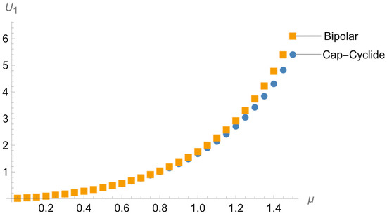
Figure 3. Radial part $U_1$ of the flux function for the cap-cyclide geometry with $k=0.001$ compared to the bipolar case with $k=1$.

Figure 4. Angular part $V_2$ of the flux function for the cap-cyclide geometry with $k=0.001$ compared to the bipolar case with $k=1$.

8. Conclusions

The availability of an analytical solution will make it possible to explicitly write down the poloidal components of the magnetic field and the Green function in the cap-cyclide coordinates. This will eventually lead to the implementation of a semi-analytical plasma equilibrium code that will be used either to design new experiments or to determine some of the most important internal parameters in current experiments by opportune fitting of the experimental data [21], such as the plasma current density and the volume integral of the kinetic pressure. Of course, at present, a large number of different numerical codes are used to calculate the internal quantities of plasma [24,25,26]. Since all these codes currently work with a good degree of reliability, the question immediately arises as to why use the “spectral” approach and what the possible advantages might be. The spectral approach, of course, is not a feature of this article; on the contrary, it has already been used earlier to solve various problems [27,28], including in the framework of plasma experiments [21,29,30]. The most important advantage of the analytical approach is that the solution intrinsically separates “external” sources from internal ones. Having a set of magnetic measurements around the plasma columns will make it possible to forget about any “noise” introduced by external sources, such as external coils and passive metal structures. The intrinsic strength of this approach was demonstrated for the first time in the JET tokamak, which made it possible to understand the possibility of having X-mode configurations [31,32]. In the future, looking at reactor machines, when magnetic probes are far from the plasma and other active diagnostic tools are difficult to implement, having a robust analytical solution to the equilibrium will be a fundamental aspect.

References

- Grad, H.; Rubin, H. Hydromagnetic equilibria and force free fileds. J. Nucl. Energy 1958, 7, 284. [Google Scholar]
- Shafranov, V.D. Equilibrium of a plasma toroid in a magnetic field. Sov. Phys. JETP 1960, 37, 775. [Google Scholar]
- Mukhovatov, V.S.; Shafranov, V.D. Plasma equilibrium in a Tokamak. Nucl. Fusion 1971, 11, 605. [Google Scholar] [CrossRef]
- Bateman, G. MHD Instabilities; MIT Press: Cambridge, MA, USA, 1978. [Google Scholar]
- Neumann, C. Theorie der Elektricitäts—Und Wärme-Vertheilung in einem Ringe; Verlag der buchhdlg des Weisenhauses: Halle, Germany, 1864. [Google Scholar]
- Böcher, M. Üeber Die Reihenentwickelungen Der Potential Theorie; Druck und Verlag von B. G. Teubner: Leipzig, Germany, 1894. [Google Scholar]
- Wangerin, A. Theorie des Potentials und der Kugelfunktionen; G. J. Gfischen’sche Verlagshandlung: Leipzig, Germany, 1909. [Google Scholar]
- Moon, P.; Spencer, D.E. Field Theory Handbook: Including Coordinate Systems, Differential Equations and Their Solutions; Springer: Berlin/Heidelberg, Germany, 2012. [Google Scholar]
- Fock, V.A. Skin effect in a ring. Fiz. Zh. Sov. 1932, 1, 215. [Google Scholar]
- Lebedev, N. The functions associated with a ring of oval cross-section. Tekh. Fiz. 1937, 4, 3. [Google Scholar]
- Honma, T.; Kito, M.; Kaji, I.; Seki, M. The vacuum poloidal flux functions satisfying of the Grad–Shafranov equation in the flat-ring cyclide coordinate system. Hokkaido Daigaku Kogakubu Kenkyu Hokoku 1979, 94, 123. [Google Scholar]
- Aikawa, I.K.; Takahara, M. Wangerin Functions; Report of Faculty of Engineering 26; Yamanashi University: Yamanashi, Japan, 1975; p. 126. [Google Scholar]
- Crisanti, F. Analytical solution of the Grad Shafranov equation in an elliptical prolate geometry. J. Plasma Phys. 2019, 85, 905850210. [Google Scholar] [CrossRef]
- Lupica, A.; Cesarano, C.; Crisanti, F.; Ishkhanyan, A. Analitical solution of the three-dimensional Laplace equation in terms of linear combinations of hypergeometric functions. Mathematics 2021, 9, 3316. [Google Scholar] [CrossRef]
- Ronveaux, A. Heun’s Differential Equations; Oxford University Press: Oxford, UK, 1995. [Google Scholar]
- Slavyanov, S.Y.; Lay, W. Special Functions; Oxford University Press: Oxford, UK, 2000. [Google Scholar]
- Ishkhanyan, A.M. Generalized hypergeometric solutions of the Heun equation. Theor. Math. Phys. 2020, 202, 1. [Google Scholar] [CrossRef]
- Letessier, J. Co-recursive associated Jacobi polynomials. J. Comput. Appl. Math. 1995, 57, 203. [Google Scholar] [CrossRef]
- Ishkhanyan, T.A.; Shahverdyan, T.A.; Ishkhanyan, A.M. Expansions of the solutions of the general Heun equation governed by two-term recurrence relations for coefficients. Adv. High Energy Phys. 2018, 2018, 4263678. [Google Scholar] [CrossRef]
- Ishkhanyan, A.M. Appell hypergeometric expansions of the solutions of the general Heun equation. Constr. Approx. 2019, 49, 445–459. [Google Scholar] [CrossRef]
- Alladio, F.; Crisanti, F. Analysis of MHD equilibria by toroidal multipolar expansions. Nucl. Fusion 1986, 26, 1143. [Google Scholar] [CrossRef]
- Olver, F.W.J.; Lozier, D.W.; Boisvert, R.F.; Clark, C.W. NIST Handbook of Mathematical Functions; Cambridge University Press: New York, NY, USA, 2010. [Google Scholar]
- Wolfram, S. In Less than a Year, so Much New: Launching Version 12.1 of Wolfram Language & Mathematica. Available online: https://writings.stephenwolfram.com/2020/03/in-less-than-a-year-so-much-new-launching-version-12-1-of-wolfram-language-mathematica/ (accessed on 19 March 2023).
- Albanese, R.; Villone, F. The linearized CREATE-L plasma response model for the control of current, position and shape in tokamaks. Nucl. Fusion 1998, 38, 723. [Google Scholar] [CrossRef]
- Lao, L.L.; John, H.S.; Stambaugh, R.; Kellman, A.; Pfeiffer, W. Reconstruction of current profile parameters and plasma shapes in tokamaks. Nucl. Fusion 1985, 25, 1611. [Google Scholar] [CrossRef]
- Albanese, R.; Ambrosino, R.; Mattei, M. CREATE-NL+: A robust control-oriented free boundary dynamic plasma equilibrium solver. Fusion Eng. Des. 2015, 664, 96–97. [Google Scholar] [CrossRef]
- Mahariq, I.; Kuzuoglu, M.; Tarman, H.; Kurt, H. Photonic Nanojet Analysis by Spectral Element Method. IEEE Photonic J. 2014, 6, 5. [Google Scholar] [CrossRef]
- Mahariq, I. On the application of the spectral element method in electromagnetic problems involving domain decomposition. Turk. J. Electr. Eng. Comput. Sci. 2017, 25, 1059–1069. [Google Scholar] [CrossRef]
- Atanasiu, C.V.; Günter, S.; Lackner, K.; Miron, I.G. Analytical solutions to the Grad–Shafranov equation. Phys. Plasmas 2004, 11, 3510. [Google Scholar] [CrossRef]
- Guazzotto, L.; Freidberg, J.P. A family of analytic equilibrium solutions for the Grad–Shafranov equation. Phys. Plasmas 2007, 14, 112508. [Google Scholar] [CrossRef]
- Alladio, F.; Crisanti, F.; Lazzaro, E.; Tanga, A. Observation High βp Effect in JET Discharge. Bull. Am. Phys. Soc. 1984, F11, 3. [Google Scholar]
- Alladio, F.; Crisanti, F.; Marinucci, M.; Micozzi, P.; Tanga, A. Analysis of tokamak configurations using the toroidal multipole method. Nucl. Fusion 1991, 31, 739. [Google Scholar] [CrossRef]
Disclaimer/Publisher’s Note: The statements, opinions and data contained in all publications are solely those of the individual author(s) and contributor(s) and not of MDPI and/or the editor(s). MDPI and/or the editor(s) disclaim responsibility for any injury to people or property resulting from any ideas, methods, instructions or products referred to in the content. |
© 2023 by the authors. Licensee MDPI, Basel, Switzerland. This article is an open access article distributed under the terms and conditions of the Creative Commons Attribution (CC BY) license (https://creativecommons.org/licenses/by/4.0/).