Threshold Analysis of a Stochastic SIRS Epidemic Model with Logistic Birth and Nonlinear Incidence

Abstract

The paper mainly investigates a stochastic SIRS epidemic model with Logistic birth and nonlinear incidence. We obtain a new threshold value ($R_0^m$) through the Stratonovich stochastic differential equation, different from the usual basic reproduction number. If $R_0^m<1$, the disease-free equilibrium of the illness is globally asymptotically stable in probability one. If $R_0^m>1$, the disease is permanent in the mean with probability one and has an endemic stationary distribution. Numerical simulations are given to illustrate the theoretical results. Interestingly, we discovered that random fluctuations can suppress outbreaks and control the disease.

1. Introduction

In the past few decades, researchers have provided various SIR models to study the spread of epidemics [1,2,3,4,5]. For example, Beretta and Takeuchi [1] proposed a deterministic SIR model with varying population sizes, and Lu et al. [2] analyzed a SIR epidemic model with horizontal and vertical transmission. In practice, the persistence of infectious diseases and disease-related deaths may lead to changes in birth rates as the population size increases toward its carrying capacity. In other words, these SIR models should consider density-dependent limited growth. Suppose that the total population $N\left(t\right)$ can be divided into three compartments at time t: susceptible $S\left(t\right)$, infectious $I\left(t\right)$, and removed $R\left(t\right)$. Zhang, Li, and Ma [3] introduced a SIR epidemic model with Logistic birth as follows

$$\left\{\begin{array}{cc}\hfill \mathrm{d}S\left(t\right)& =\left[\left(b-r\frac{N\left(t\right)}{K}\right)N\left(t\right)-\mu S\left(t\right)-\eta S\left(t\right)I\left(t\right)\right]\mathrm{d}t,\hfill \\ \hfill \mathrm{d}I\left(t\right)& =\left[\eta S\left(t\right)I\left(t\right)-\left(\mu +\varphi +\kappa \right)I\left(t\right)\right]\mathrm{d}t,\hfill \\ \hfill \mathrm{d}R\left(t\right)& =\left[\varphi I\left(t\right)-\mu R\left(t\right)\right]\mathrm{d}t,\hfill \end{array}\right.$$

(1)

where K is the environmental capacity, b is the birth rate, $\eta$ is the exposure rate, $\mu$ is the natural mortality rate, $r(=b-\mu )$ is the intrinsic rate, $\kappa$ is the mortality rate due to disease, and $\varphi$ is the recovery rate of the infected.

For some diseases, the recovered individuals will lose immunity after a certain period and become susceptible again. The SIRS model can be used to describe this phenomenon [6,7,8,9]. However, most SIRS models often ignore the density-dependent demographics and heterogeneous populations. Inspired by the above models, we propose a deterministic SIRS model with Logistic birth and a nonlinear incidence rate, which is formed by

$$\left\{\begin{array}{cc}\hfill \mathrm{d}S\left(t\right)& =\left[\left(b-r\frac{N\left(t\right)}{K}\right)N\left(t\right)-\mu S\left(t\right)-\eta f(S\left(t\right),I\left(t\right),R\left(t\right))+\psi R\left(t\right)\right]\mathrm{d}t,\hfill \\ \hfill \mathrm{d}I\left(t\right)& =\left[\eta f(S\left(t\right),I\left(t\right),R\left(t\right))-\left(\mu +\varphi +\kappa \right)I\left(t\right)\right]\mathrm{d}t,\hfill \\ \hfill \mathrm{d}R\left(t\right)& =\left[\varphi I\left(t\right)-(\mu +\psi )R\left(t\right)\right]\mathrm{d}t,\hfill \end{array}\right.$$

(2)

where f is a positive function, and $\psi$ denotes the immunity loss rate of the recovered. The model (1) is a special case of model (2) with $\psi =0$ and $f\left(S\right(t),I(t),R(t\left)\right)=S\left(t\right)I\left(t\right)$.

In the real world, all dynamic systems are affected by environmental noise [10,11,12,13]. It is necessary to study a stochastic SIRS epidemic model with Logistic birth and a nonlinear incidence rate is necessary. Considering the effect of random perturbations, we assume that the perturbations in the environment are expressed as a parameter $\eta$ change to the random variable $\eta \to \eta +\sigma \mathrm{d}B\left(t\right)$ and obtain the following stochastic SIRS model

$$\left\{\begin{array}{cc}\hfill \mathrm{d}S\left(t\right)=& \left[\left(b-r\frac{N\left(t\right)}{K}\right)N\left(t\right)-\mu S\left(t\right)-\eta f(S\left(t\right),I\left(t\right),R\left(t\right))+\psi R\left(t\right)\right]\mathrm{d}t\hfill \\ \hfill & -\sigma f\left(S\right(t),I(t),R(t\left)\right)\mathrm{d}B\left(t\right),\hfill \\ \hfill \mathrm{d}I\left(t\right)=& \left[\eta f\left(S\right(t),I(t),R(t\left)\right)-(\mu +\varphi +\kappa )I\left(t\right)\right]\mathrm{d}t+\sigma f(S\left(t\right),I\left(t\right),R\left(t\right))\mathrm{d}B\left(t\right),\hfill \\ \hfill \mathrm{d}R\left(t\right)=& \left[\varphi I\left(t\right)-(\mu +\psi )R\left(t\right)\right]\mathrm{d}t,\hfill \end{array}\right.$$

(3)

where $\sigma$ represents the intensity of white environmental noise and $B\left(t\right)$ is a one-dimensional standard Brownian motion. Obviously, model (2) is also a special case of model (3) for $\sigma =0$. This paper aims to analyze the asymptotic properties of the stochastic model (3) by studying global stability, persistence, and stationary distribution.

In epidemiological studies, the basic reproduction number is an indicative factor in considering whether a disease is endemic or not. In this paper, we introduce a new threshold value through the Stratonovich stochastic differential equation and further analyze the dynamic properties of model (3).

2. Preliminaries

Denote ${\mathbb{R}}_{+}^3=\{x=\left(x_1,x_2,x_3\right)\in {\mathbb{R}}^3:x_i>0,1\le i\le 3\}$, and $\mathsf{\Theta }=\left\{\right(S,I,R):S\ge 0,I\ge 0,R\ge 0,S+I+R>0\}$. Let $(\mathsf{\Omega },\mathcal{F},{\left\{{\mathcal{F}}_t\right\}}_{t\ge 0},\mathbb{P})$ be a complete probability space with a filtration ${\left\{{\mathcal{F}}_t\right\}}_{t\ge 0}$ satisfying the usual conditions (${\mathcal{F}}_0$ is increasing and right continuous while ${\mathcal{F}}_0$ contains all $\mathbb{P}$-null sets). From [14], we give Itô’s formula for general stochastic differential equations. Consider a 3-dimensional stochastic differential equation

$$dW\left(t\right)=f(W\left(t\right),t)dt+g(W\left(t\right),t)dB\left(t\right)\mathrm{for}t\ge t_0$$

with an initial value $W\left(0\right)=W_0\in {\mathbb{R}}^3$, $B\left(t\right)$ denotes a 3-dimensional vector of standard Brownian motions defined on the complete probability space. Let the function $V(W,t)\in C^{2,1}({\mathbb{R}}^3\times [t_0,\infty );{\mathbb{R}}_{+})$ be continuously twice differentiable in W and once in t. The differential operator L is defined as

$$L=\frac{\partial }{\partial t}+\sum _{i=1}^3{f}_i(W,t)\frac{\partial }{\partial W_i}+\frac{1}{2}\sum _{i,j=1}^3{\left[g^T(W,t)g(W,t)\right]}_{ij}\frac{{\partial }^2}{\partial W_i\partial W_j}.$$

Let a function $V\in C^{2,1}({\mathbb{R}}^3\times [t_0,\infty );{\mathbb{R}}_{+})$, we obtain

$$LV(W,t)=V_t(W,t)+V_W(W,t)f(W,t)+\frac{1}{2}trace\left[g^T(W,t)V_{WW}(W,t)g(W,t)\right],$$

where $V_t=\frac{\partial V}{\partial t},V_W=(\frac{\partial V}{\partial W_1},\frac{\partial V}{\partial W_2},\frac{\partial V}{\partial W_3}),V_{WW}={\left(\frac{{\partial }^{2}V}{\partial W_i\partial W_j}\right)}_{3\times 3}$. Then,

$$dV(W\left(t\right),t)=LV(W\left(t\right),t)dt+V_W(W\left(t\right),t)g(W\left(t\right),t)dB\left(t\right).$$

Lemma 1. 

[15] The Itô stochastic differential equation (SDE)

$$\left\{\begin{array}{c}d{W}_t=f(t,W\left(t\right))dt+g(t,W\left(t\right))dB\left(t\right),\hfill \\ W\left(0\right)=W_0,\hfill \end{array}\right.$$

is equivalent (has the same solution) as the Stratonovich SDE

$$\left\{\begin{array}{c}dW\left(t\right)=\left(f(t,W\left(t\right))-\frac{1}{2}\frac{\partial g(t,W(t\left)\right)}{dx}g(t,W\left(t\right))\right)dt+g(t,W\left(t\right))\circ dB\left(t\right),\hfill \\ W\left(0\right)=W_0.\hfill \end{array}\right.$$

In models (2) and (3), suppose that the function $f(S,I,R)$ satisfies the following conditions:

$\left({\mathbf{H}}_1\right)$$f(S,I,R)$ is nonnegative and twice continuously differentiable for all $(S,I,R)\in \mathsf{\Theta }$, $\partial f(S,I,R)/\partial S>0$ and $\partial f(S,I,R)/\partial R<0$.

$\left({\mathbf{H}}_2\right)$$f(S,0,R)=f(0,I,R)\equiv 0$, $f(S,I,R)/I\le \partial f(S_0,0,0)/\partial I$ for any $(S,I,R)\in \mathsf{\Theta }$, and $\partial f(S_0,0,0)/\partial I>0$, where $S_0=K$.

Under assumptions $\left({\mathbf{H}}_1\right)$ and $\left({\mathbf{H}}_2\right)$, it is obvious that

$$\frac{\partial f(0,I,R)}{\partial I}=\frac{\partial f(0,I,R)}{\partial R}=\frac{\partial f(S,0,R)}{\partial S}=\frac{\partial f(S,0,R)}{\partial R}\equiv 0,(S,I,R)\in \mathsf{\Theta }.$$

Lemma 2. 

For any constants $p>q>0$, let $D=\left\{\right(S,I,R):S>0,I>0,R>0,q\le S+I+R\le p\}$. Under $\left({\mathbf{H}}_1\right)$ and $\left({\mathbf{H}}_2\right)$, we have

$$\begin{array}{ccc}& & \underset{(S,I,R)\in D}{max}\left\{\frac{f(S,I,R)}{S},\frac{f(S,I,R)}{I}\right\}<\infty ,\hfill \\ & & \underset{(S,I,R)\in D}{max}\left\{\left|\frac{1}{I}\frac{\partial f(S,I,R)}{\partial I}-\frac{f(S,I,R)}{I^2}\right|,\left|\frac{1}{I}\frac{\partial f(S,I,R)}{\partial S}\right|\right\}<\infty .\hfill \end{array}$$

The proof of Lemma 2 is similar to that of Lemma 2.1 in Ramziya et al. [16]. Denote $M_S\triangleq {max}_{\mathsf{\Gamma }}\{f(S,I,R)/S\}$. Define a bounded set

$$\mathsf{\Gamma }=\left\{(S,I,R):S>0,I>0,R>0,K\left(1-\frac{\kappa }{r}\right)\le S+I+R\le K\right\}.$$

(4)

Lemma 3. 

Suppose that $\left({\mathbf{H}}_1\right)$ and $\left({\mathbf{H}}_2\right)$ hold.

(i) The region Γ is almost surely positive invariant in model (3).

(ii) For any initial value $(S\left(0\right),I\left(0\right),R\left(0\right))\in R_{+}^3$, model (3) has a unique positive solution $\left(S\right(t),I(t),R(t\left)\right)$ on $t>0$. That is to say, the solution will remain in a compact subset of Γ. Furthermore,

$$K\left(1-\frac{\kappa }{r}\right)\le \underset{t\to \infty }{lim\; inf}\left(S\left(t\right)+I\left(t\right)+R\left(t\right)\right)\le \underset{t\to \infty }{lim\; sup}(S\left(t\right)+I\left(t\right)+R\left(t\right))\le S_0.$$

The proof of Lemma 3 can be obtained using a similar method in Cai et al. [17]. The lemma shows that we can study the dynamic properties of model (3) in the bounded set $\mathsf{\Gamma }$. To obtain the basic reproduction number of model (3), we define a $C^2$ function $V:V\left(S\right(t),I(t\left)\right)=ln\left(S\right(t),I(t\left)\right)$. By using Itô’s formula, it follows that

$$\begin{array}{cc}\hfill \mathrm{d}lnS=& \left[\frac{1}{S}\left(\left(b-r\frac{N}{K}\right)N-\mu S-\eta f(S,I,R)+\psi R\right)-\frac{1}{2}{\sigma }^2{f}^2(S,I,R)\frac{1}{S^2}\right]\mathrm{d}t\hfill \\ \hfill & -\sigma f(S,I,R)\frac{1}{S}\mathrm{d}B\left(t\right),\hfill \\ \hfill \mathrm{d}lnI=& \left[\frac{1}{I}(\eta f(S,I,R)-(\mu +\varphi +\kappa )I)-\frac{1}{2}{\sigma }^2{f}^2(S,I,R)\frac{1}{I^2}\right]\mathrm{d}t+\sigma f(S,I,R)\frac{1}{I}\mathrm{d}B\left(t\right).\hfill \end{array}$$

Thus, we have

$$\begin{array}{cc}\hfill \mathrm{d}S=& \left[\left(b-r\frac{N}{K}\right)N-\mu S-\eta f(S,I,R)+\psi R-\frac{1}{2}{\sigma }^2{f}^2(S,I,R)\frac{1}{S}\right]\mathrm{d}t-\sigma f(S,I,R)\mathrm{d}B\left(t\right),\hfill \\ \hfill \mathrm{d}I=& \left[\eta f(S,I,R)-(\mu +\varphi +\kappa )I-\frac{1}{2}{\sigma }^2{f}^2(S,I,R)\frac{1}{I}\right]\mathrm{d}t+\sigma f(S,I,R)\mathrm{d}B\left(t\right).\hfill \end{array}$$

(5)

We transform (5) into a Stratonovich SDE and obtain

$$\begin{array}{cc}\hfill \mathrm{d}S=& [\left(b-r\frac{N}{K}\right)N-\mu S-\eta f(S,I,R)+\psi R-\frac{1}{2}{\sigma }^2{f}^2(S,I,R)\frac{1}{S}\hfill \\ \hfill & -\frac{1}{2}{\sigma }^{2}f(S,I,R)\frac{\partial f(S,I,R)}{\partial S}]\mathrm{d}t-\sigma f(S,I,R)\circ \mathrm{d}B\left(t\right),\hfill \\ \hfill \mathrm{d}I=& \left[\eta f(S,I,R)-(\mu +\varphi +\kappa )I-\frac{1}{2}{\sigma }^2{f}^2(S,I,R)\frac{1}{I}-\frac{1}{2}{\sigma }^{2}f(S,I,R)\frac{\partial f(S,I,R)}{\partial I}\right]\mathrm{d}t\hfill \\ \hfill & +\sigma f(S,I,R)\circ \mathrm{d}B\left(t\right).\hfill \end{array}$$

Taking the mean value of the above equations derives

$$\begin{array}{cc}\hfill E\left(\mathrm{d}S\right)=& [\left(b-r\frac{N}{K}\right)N-\mu S-\eta f(S,I,R)+\psi R-\frac{1}{2}{\sigma }^2{f}^2(S,I,R)\frac{1}{S}\hfill \\ \hfill & -\frac{1}{2}{\sigma }^{2}f(S,I,R)\frac{\partial f(S,I,R)}{\partial S}]\mathrm{d}t\hfill \\ \hfill E\left(\mathrm{d}I\right)=& \left[\eta f(S,I,R)-(\mu +\varphi +\kappa )I-\frac{1}{2}{\sigma }^2{f}^2(S,I,R)\frac{1}{I}-\frac{1}{2}{\sigma }^{2}f(S,I,R)\frac{\partial f(S,I,R)}{\partial I}\right]\mathrm{d}t.\hfill \end{array}$$

As a result, the study of model (3) can be turned into

$$\left\{\begin{array}{cc}\hfill E\left(\mathrm{d}S\right)=& [\left(b-r\frac{N}{K}\right)N-\mu S-\eta f(S,I,R)+\psi R-\frac{1}{2}{\sigma }^2{f}^2(S,I,R)\frac{1}{S}\hfill \\ \hfill & -\frac{1}{2}{\sigma }^{2}f(S,I,R)\frac{\partial f(S,I,R)}{\partial S}]\mathrm{d}t,\hfill \\ \hfill E\left(\mathrm{d}I\right)=& \left[\eta f(S,I,R)-(\mu +\varphi +\kappa )I-\frac{1}{2}{\sigma }^2{f}^2(S,I,R)\frac{1}{I}-\frac{1}{2}{\sigma }^{2}f(S,I,R)\frac{\partial f(S,I,R)}{\partial I}\right]\mathrm{d}t,\hfill \\ \hfill \mathrm{d}R=& \left[\varphi I-(\mu +\psi )R\right]\mathrm{d}t,\hfill \end{array}\right.$$

(6)

Denote $x={(I,S,R)}^{\mathrm{T}}$. Then system (6) can be given as

$$x^{\prime }=\mathcal{F}\left(x\right)-\mathcal{V}\left(x\right),$$

where

$$\mathcal{F}\left(x\right)=\left(\begin{array}{c}\eta f(S,I,R)-\frac{1}{2}{\sigma }^{2}f(S,I,R)\frac{\partial f(S,I,R)}{\partial I}\\ 0\\ 0\end{array}\right);$$

$$\mathcal{V}\left(x\right)=\left(\begin{array}{c}(\mu +\varphi +\kappa )I+\frac{1}{2}{\sigma }^2{f}^2(S,I,R)\frac{1}{I}\\ -\left(b-r\frac{N}{K}\right)N+\mu S+\eta f(S,I,R)-\psi R+\frac{1}{2}{\sigma }^2{f}^2(S,I,R)\frac{1}{S}+\frac{1}{2}{\sigma }^{2}f(S,I,R)\frac{\partial f(S,I,R)}{\partial S}\\ -\varphi I\left(t\right)+(\mu +\psi )R\left(t\right)\end{array}\right).$$

Through the calculation, model (3) has a unique disease-free equilibrium $E_0=(S_0,0,0)$, which is also that of model (6). The Jacobian matrices of $\mathcal{F}\left(x\right)$ and $\mathcal{V}\left(x\right)$ at $E_0$ are denoted as F and V, respectively. Under the assumption $\left({\mathbf{H}}_2\right)$, by the calculation, there are

$$\begin{array}{c}\hfill F=\left(\begin{array}{ccc}\eta \frac{\partial f(S_0,0,0)}{\partial I}-\frac{1}{2}{\sigma }^2{\left(\frac{\partial f(S_0,0,0)}{\partial I}\right)}^2& 0& 0\\ 0& 0& 0\\ 0& 0& 0\end{array}\right)\end{array}$$

and

$$\begin{array}{c}\hfill V=\left(\begin{array}{ccc}\mu +\varphi +\kappa & 0& 0\\ -b+2r+\eta \frac{\partial f(S_0,0,0)}{\partial I}& r& -b+2r-\psi \\ -\varphi & 0& \mu +\psi \end{array}\right).\end{array}$$

Then the basic reproduction number of model (6) is

$$\begin{array}{cc}\hfill R_0^m& =\rho \left(F{V}^{-1}\right)=\frac{\partial f(S_0,0,0)}{\partial I}\frac{\eta }{\mu +\varphi +\kappa }-{\left(\frac{\partial f(S_0,0,0)}{\partial I}\right)}^2\frac{{\sigma }^2}{2(\mu +\varphi +\kappa )}\hfill \\ \hfill & =R_0-{\left(\frac{\partial f(S_0,0,0)}{\partial I}\right)}^2\frac{{\sigma }^2}{2(\mu +\varphi +\kappa )},\hfill \end{array}$$

which is also that of model (3). In view of $\sigma =0$, model (6) is then transformed into model (2). The basic reproduction number of model (2) is easily obtained as

$$R_0=\frac{\partial f(S_0,0,0)}{\partial I}\frac{\eta }{\mu +\varphi +\kappa }.$$

In the following, we present some properties of model (2).

Theorem 1. 

The disease-free equilibrium $E_0=(K,0,0)$ of model (2) is locally asymptotically stable if $R_0<1$.

Proof. 

Given that assumptions $\left({\mathbf{H}}_1\right)$ and $\left({\mathbf{H}}_2\right)$ hold, the Jacobian matrix of model (2) evaluated at $E_0$ is

$$J\left(E_0\right)=\left(\begin{array}{ccc}-r& b-2r& b-2r+\psi \\ 0& -(\mu +\kappa +\varphi )& 0\\ 0& \varphi & -(\mu +\psi )\end{array}\right).$$

Thus, the characteristic equation at $E_0$ is

$$(\lambda +r)(\lambda +\mu +\kappa +\varphi )(\lambda +\mu +\psi )=0,$$

which has eigenvalues ${\lambda }_1=-r<0,{\lambda }_2=-(\mu +\kappa +\varphi )<0$ and ${\lambda }_3=-(\mu +\psi )<0$. Therefore, the disease-free equilibrium $E_0$ is locally asymptotically stable. The proof is complete. □

Theorem 2. 

If $R_0>1$, model (2) has a unique endemic equilibrium $E^{*}=(S^{*},I^{*},R^{*})$, which is locally asymptotically stable.

Proof. 

The Jacobian matrix of model (2) evaluated at $E^{*}$ is

$$J\left(E^{*}\right)=\left(\begin{array}{ccc}A-\mu -\eta \frac{\partial f(S^{*},I^{*},R^{*})}{\partial S}& A-\eta \frac{\partial f(S^{*},I^{*},R^{*})}{\partial I}& A-\eta \frac{\partial f(S^{*},I^{*},R^{*})}{\partial R}+\psi \\ \eta \frac{\partial f(S^{*},I^{*},R^{*})}{\partial S}& \eta \frac{\partial f(S^{*},I^{*},R^{*})}{\partial I}-(\mu +\kappa +\varphi )& \eta \frac{\partial f(S^{*},I^{*},R^{*})}{\partial R}\\ 0& \varphi & -(\mu +\psi )\end{array}\right),$$

where $A=b-2\frac{r}{K}(S^{*}+I^{*}+R^{*})$. The characteristic polynomial of $J\left(E^{*}\right)$ is

$${\lambda }^3+a_1{\lambda }^2+a_2\lambda +a_3=0,$$

where

$$\begin{array}{cc}\hfill a_1=& A-\eta \frac{\partial f(S^{*},I^{*},R^{*})}{\partial S}+\eta \frac{\partial f(S^{*},I^{*},R^{*})}{\partial I}-3\mu -\kappa -\varphi -\psi >0,\hfill \\ \hfill a_2=& \left(A-\mu -\eta \frac{\partial f(S^{*},I^{*},R^{*})}{\partial S}\right)\left(\eta \frac{\partial f(S^{*},I^{*},R^{*})}{\partial I}-2\mu -\kappa -\varphi -\psi \right)\hfill \\ \hfill & +\left(\eta \frac{\partial f(S^{*},I^{*},R^{*})}{\partial I}-\mu -\kappa -\varphi \right)(-\mu -\psi )-\eta \varphi \frac{\partial f(S^{*},I^{*},R^{*})}{\partial R}\hfill \\ \hfill & +\left(-A+\eta \frac{\partial f(S^{*},I^{*},R^{*})}{\partial I}\right)\eta \frac{\partial f(S^{*},I^{*},R^{*})}{\partial S}>0,\hfill \\ \hfill a_3=& -\left(A-\mu -\eta \frac{\partial f(S^{*},I^{*},R^{*})}{\partial S}\right)(\left(\eta \frac{\partial f(S^{*},I^{*},R^{*})}{\partial I}-\mu -\kappa -\varphi \right)(-\mu -\psi )\hfill \\ \hfill & -\eta \varphi \frac{\partial f(S^{*},I^{*},R^{*})}{\partial R})+\eta \frac{\partial f(S^{*},I^{*},R^{*})}{\partial S}(\left(-A+\eta \frac{\partial f(S^{*},I^{*},R^{*})}{\partial I}\right)(\mu +\psi )\hfill \\ \hfill & +\left(-A+\eta \frac{\partial f(S^{*},I^{*},R^{*})}{\partial R}-\psi \right)\varphi )>0.\hfill \end{array}$$

We can verify that $a_1{a}_2-a_3>0$. Therefore, $E^{*}$ is locally asymptotically stable by employing the Routh–Hurwitz criterion. □

3. Existence and Uniqueness of the Global Positive Solution

Theorem 3. 

There is a unique solution $\left(S\right(t),I(t),R(t\left)\right)$ of model (3) on $t\ge 0$ for any given initial value $\left(S\right(0),I(0),$ $R\left(0\right))\in R_{+}^3$, and this solution remains in $R_{+}^3$ with probability one.

Proof. 

The coefficients of model (3) are locally Lipschitz continuous. For any given initial value $\left(S\right(0),I(0),R(0\left)\right)$, there exists a unique local solution $(S\left(t\right),I\left(t\right),R\left(t\right))\in {\mathbb{R}}_{+}^3$ on $t\in [0,{\tau }_e)$, where ${\tau }_e$ denotes the explosion time. To prove the existence of a unique global solution to the stochastic model (3), it is only necessary to prove ${\tau }_e=\infty a.s.$.

Let $l_0>0$ be sufficiently large, such that $S\left(0\right),I\left(0\right)$ and $R\left(0\right)$ all lie within the interval $[\frac{1}{l_0},l_0]$. For each integer $l\ge l_0$, define a stopping time

$${\tau }_l=inf\left\{t\in [0,{\tau }_e):min\{S\left(t\right),I\left(t\right),R\left(t\right)\}\le \frac{1}{l}\mathrm{or}max\{S\left(t\right),I\left(t\right),R\left(t\right)\}\ge l\right\},$$

where $inf\varnothing =\infty$ (as usual ∅ = the empty set). Clearly, ${\tau }_l$ increases as $l\to \infty$. Let ${\tau }_{\infty }={lim}_{l\to \infty }{\tau }_l$, then ${\tau }_{\infty }\le {\tau }_e$ a.s. If ${\tau }_{\infty }=\infty$ a.s., then ${\tau }_e=\infty$ a.s. Otherwise, there exists a pair of constants $T>0$ and $ϵ\in (0,1)$, such that $\mathbb{P}\{{\tau }_{\infty }\le T\}>ϵ$. Hence, there exists an integer $l_1\ge l_0$, such that

$$\mathbb{P}\left\{{\tau }_l\le T\right\}\ge ϵ,\forall l\ge l_1.$$

(7)

Define a Lyapunov function by

$$V(S,I,R)=(S-1-lnS)+(I-1-lnI)+(R-1-lnR).$$

For any $l\ge l_0$ and $t\in [0,{\tau }_l)$, applying Itô’s formula to V, we obtain

$$dV(S,I,R)=LV(S,I,R)dt+\sigma f(S,I,R)\left(\frac{1}{S}-\frac{1}{I}\right)dB\left(t\right),$$

(8)

where

$$\begin{array}{cc}\hfill LV(S,I,R)=& \left(1-\frac{1}{S}\right)\left(\left(b-r\frac{N}{K}\right)N-\mu S-\eta f(S,I,R)+\psi R\right)+\frac{{\sigma }^2}{2}{f}^2(S,I,R)\frac{1}{S^2}\hfill \\ \hfill & +\left(1-\frac{1}{I}\right)(\eta f(S,I,R)-(\mu +\varphi +\kappa )I)+\frac{{\sigma }^2}{2}{f}^2(S,I,R)\frac{1}{I^2}\hfill \\ \hfill & +\left(1-\frac{1}{R}\right)(\varphi I-(\mu +\psi )R)\hfill \\ \hfill =& r\left(1-\frac{N}{K}\right)N-\frac{N}{S}\left(b-r\frac{N}{K}\right)+3\mu +\eta \frac{f(S,I,R)}{S}-\frac{\psi R}{S}+\frac{1}{2}{\sigma }^2{\left(\frac{f(S,I,R)}{S}\right)}^2\hfill \\ \hfill & -\kappa I-\eta \frac{f(S,I,R)}{I}+\varphi +\kappa +\frac{1}{2}{\sigma }^2{\left(\frac{f(S,I,R)}{I}\right)}^2-\frac{\varphi I}{R}+\psi \hfill \\ \hfill \le & r\left(1-\frac{N}{K}\right)N+3\mu +\eta M_S+\frac{1}{2}{\sigma }^2{M}_S^2+\varphi +\kappa +\frac{1}{2}{\sigma }^2{\left(\frac{\partial f(S_0,0,0)}{\partial I}\right)}^2+\psi \hfill \\ \hfill :=& K_1,\hfill \end{array}$$

where $K_1$ is a positive constant. Then according to (8), we have

$$dV(S,I,R)=K_{1}dt+\sigma f(S,I,R)\left(\frac{1}{S}-\frac{1}{I}\right)dB\left(t\right).$$

(9)

Integrating both sides of (9) from 0 to ${\tau }_l\wedge T$ and taking the expectation, we have

$$\begin{array}{cc}\hfill & EV(S({\tau }_l\wedge T),I({\tau }_l\wedge T),R({\tau }_l\wedge T))\hfill \\ \hfill & \le EV(S\left(0\right),I\left(0\right),R\left(0\right))+K_{1}E({\tau }_l\wedge T)+E{\int }_0^{{\tau }_l\wedge T}\sigma f(S,I,R)\left(\frac{1}{S}-\frac{1}{I}\right)dB\left(t\right)\hfill \\ \hfill & \le V(S\left(0\right),I\left(0\right),R\left(0\right))+K_{1}T.\hfill \end{array}$$

(10)

Let ${\mathsf{\Omega }}_l=\{\omega :{\tau }_l\le T\}$ for $l\ge l_0$. From (7) we have $P\left({\mathsf{\Omega }}_l\right)\ge \epsilon$. For every $\omega \in {\mathsf{\Omega }}_l$, we learn $S({\tau }_l,\omega )$ or $I({\tau }_l,\omega )$ or $R({\tau }_l,\omega )$ equals either l or $\frac{1}{l}$. Therefore, from (10), there is

$$\begin{array}{c}V(S\left(0\right),I\left(0\right),R\left(0\right))+K_{1}T\hfill \\ \ge E\left(I_{{\mathsf{\Omega }}_l}V\left(S\left({\tau }_l\wedge T\right),I\left({\tau }_l\wedge T\right),R\left({\tau }_l\wedge T\right)\right)\right)\hfill \\ =P\left({\mathsf{\Omega }}_l\right)EV\left(S\left({\tau }_l,\omega \right),I\left({\tau }_l,\omega \right),R\left({\tau }_l,\omega \right)\right)\hfill \\ \ge \epsilon \left\{(l-1-logl)\wedge \left(\frac{1}{l}-1-log\frac{1}{l}\right)\wedge (l-1-logl)\right.\hfill \\ \left.\wedge \left(\frac{1}{l}-1-log\frac{1}{l}\right)\wedge (l-1-logl)\wedge \left(\frac{1}{l}-1-log\frac{1}{l}\right)\right\},\hfill \end{array}$$

where $I_{{\mathsf{\Omega }}_l}$ is the indicator function of ${\mathsf{\Omega }}_l$. Taking $l\to \infty$ results

$$\infty >V(S\left(0\right),I\left(0\right),R\left(0\right))+K_{1}T=\infty .$$

Hence, ${\tau }_{\infty }=\infty a.s.$. It completes the proof. □

4. Global Stability of Disease-Free Equilibrium

Denote

$${\sigma }_a=\sqrt{\frac{\eta }{\partial f(S_0,0,0)/\partial I}}\mathrm{and}{\sigma }_b=\frac{\eta }{\sqrt{2(\mu +\varphi +\kappa )}}.$$

The following result reveals the asymptotic property of $E_0$ in model (3).

Theorem 4. 

Under $\left({\mathbf{H}}_1\right)$ and $\left({\mathbf{H}}_2\right)$, the disease-free equilibrium $E_0$ is globally asymptotically stable in probability one if one of the following conditions holds: (a) $R_0^m<1and\sigma \le {\sigma }_a$, or (b) $\sigma >max\{{\sigma }_a,{\sigma }_b\}.$

Proof. 

Let $k_1$ and $k_2$ be two positive constants. Define a Lyapunov function

$$V(S,I,R)=\frac{1}{2}{k}_1{\left(K-S\right)}^2+\frac{1}{k_2}{I}^{k_2}+\frac{1}{2}\frac{k_1\psi }{\varphi }{R}^2.$$

Obviously, $V(S,I,R)\ge 0$ in the region $\mathsf{\Gamma }$. Through Itô’s formula and model (3), it follows that

$$dV(S,I,R)=LV(S,I,R)dt+\sigma f(S,I,R)\left(k_1\left(K-S\right)+I^{k_2-1}\right)dB\left(t\right),$$

where

$$\begin{array}{cc}\hfill LV=& -k_1(K-S)\left(\left(b-r\frac{N}{K}\right)N-\mu S-\eta f(S,I,R)+\psi R\right)\hfill \\ \hfill & +\frac{1}{2}{k}_1{\sigma }^2{f}^2(S,I,R)+I^{k_2-1}(\eta f(S,I,R)-(\mu +\kappa +\varphi )I)\hfill \\ \hfill & +\frac{1}{2}(k_2-1){\sigma }^2{f}^2(S,I,R)I^{k_2-2}+\frac{k_1\psi }{\varphi }R(\varphi I-(\mu +\psi )R)\hfill \\ \hfill =& -k_1(K-S)\left(\left(b-r\frac{N}{K}\right)N-\mu S\right)+k_1\left(K-S\right)\eta I\frac{f(S,I,R)}{I}-k_1\left(K-S\right)\psi R\hfill \\ \hfill & +\frac{1}{2}{k}_1{\sigma }^2{I}^2{\left(\frac{f(S,I,R)}{I}\right)}^2+\eta I^{k_2}\frac{f(S,I,R)}{I}-(\mu +\kappa +\varphi )I^{k_2}\hfill \\ \hfill & +\frac{1}{2}{k}_2{\sigma }^2{\left(\frac{f(S,I,R)}{I}\right)}^2{I}^{k_2}-\frac{1}{2}{\sigma }^2{\left(\frac{f(S,I,R)}{I}\right)}^2{I}^{k_2}+k_1\psi RI-\frac{k_1\psi (\mu +\psi )R^2}{\varphi }.\hfill \end{array}$$

For any constant $\rho >0$ and $k_2\le 2$, we have

$$\begin{array}{c}\hfill I\left(t\right)\le K-S\left(t\right),I^2\le K^{2-k_2}{I}^{k_2},\mathrm{and}I(K-S)\le \frac{1}{4\rho }{I}^2+\rho {\left(K-S\right)}^2\le \frac{1}{4\rho }{K}^{2-k_2}{I}^{k_2}+\rho {(K-S)}^2.\end{array}$$

Based on the above inequalities and $\left({\mathbf{H}}_2\right)$, it yields that

$$\begin{array}{cc}\hfill LV\le & -k_1\left(K-S\right)\left(\left(b-r\frac{N}{K}\right)N-\mu S-\eta \rho (K-S)\frac{\partial f(S_0,0,0)}{\partial I}\right)-k_1\left(K-S\right)\psi R\hfill \\ \hfill & +\frac{1}{2}{k}_1{\sigma }^2{I}^2{\left(\frac{\partial f(S_0,0,0)}{\partial I}\right)}^2+\eta I^{k_2}\frac{f(S,I,R)}{I}-(\mu +\kappa +\varphi )I^{k_2}\hfill \\ \hfill & +\frac{1}{2}{k}_2{\sigma }^2{\left(\frac{\partial f(S_0,0,0)}{\partial I}\right)}^2{I}^{k_2}-\frac{1}{2}{\sigma }^2{\left(\frac{f(S,I,R)}{I}\right)}^2{I}^{k_2}+k_1\psi R(K-S)-\frac{k_1\psi (\mu +\psi )R^2}{\varphi }\hfill \\ \hfill & +k_1\eta \frac{1}{4\rho }{K}^{2-k_2}{I}^{k_2}\frac{f(S,I,R)}{I}\hfill \\ \hfill \le & -k_1(K-S)\left(\left(b-r\frac{N}{K}\right)N-\mu S-\eta \rho (K-S)\frac{\partial f(S_0,0,0)}{\partial I}\right)\hfill \\ \hfill & +I^{k_2}\left(\eta \frac{f(S,I,R)}{I}+(\mu +\kappa +\varphi )-\frac{1}{2}{\sigma }^2{\left(\frac{f(S,I,R)}{I}\right)}^2\right)+\frac{1}{2}{k}_2{\sigma }^2{\left(\frac{\partial f(S_0,0,0)}{\partial I}\right)}^2{I}^{k_2}\hfill \\ \hfill & -\frac{k_1\psi (\mu +\psi )R^2}{\varphi }+k_1\eta \frac{1}{4\rho }{K}^{2-k_2}{I}^{k_2}\frac{\partial f(S_0,0,0)}{\partial I}+\frac{1}{2}{k}_1{\sigma }^2{K}^{2-k_2}{I}^{k_2}{\left(\frac{\partial f(S_0,0,0)}{\partial I}\right)}^2\hfill \\ \hfill =& -k_1\left(K-S\right)\left(\left(b-r\frac{N}{K}\right)N-\mu S-\eta \rho (K-S)\frac{\partial f(S_0,0,0)}{\partial I}\right)\hfill \\ \hfill & +I^{k_2}\left(\eta \frac{f(S,I,R)}{I}+(\mu +\kappa +\varphi )-\frac{1}{2}{\sigma }^2{\left(\frac{f(S,I,R)}{I}\right)}^2\right)\hfill \\ \hfill & +I^{k_2}(\frac{1}{2}{k}_1{\sigma }^2{K}^{2-k_2}{\left(\frac{\partial f(S_0,0,0)}{\partial I}\right)}^2+\frac{1}{2}{k}_2{\sigma }^2{\left(\frac{\partial f(S_0,0,0)}{\partial I}\right)}^2\hfill \\ \hfill & +k_1\eta \frac{1}{4\rho }{K}^{2-k_2}\frac{\partial f(S_0,0,0)}{\partial I})-\frac{k_1\psi (\mu +\psi )R^2}{\varphi }.\hfill \end{array}$$

Denote $h\left(x\right)=\eta x-(\mu +\varphi +\kappa )-\frac{1}{2}{\sigma }^2{x}^2$. The function $h\left(x\right)$ increases for $x\in [0,\eta /{\sigma }^2]$. If $R_0^m<1$ and $\sigma \le {\sigma }_a$, then $f(S,I,R)/I\le \partial f(S_0,0,0)/\partial I\le \eta /{\sigma }^2$. We obtain

$$\begin{array}{cc}\hfill & \eta \frac{f(S,I,R)}{I}-(\mu +\varphi +\kappa )-\frac{1}{2}{\sigma }^2{\left(\frac{f(S,I,R)}{I}\right)}^2\hfill \\ \hfill & \le \eta \frac{\partial f\left(S_0,0,0\right)}{\partial I}-(\mu +\varphi +\kappa )-\frac{1}{2}{\sigma }^2{\left(\frac{\partial f\left(S_0,0,0\right)}{\partial I}\right)}^2\triangleq A_1<0,\hfill \end{array}$$

If $\sigma >max\{{\sigma }_a,{\sigma }_b\}$, we have

$$\begin{array}{cc}\hfill & \eta \frac{f(S,I,R)}{I}-(\mu +\varphi +\kappa )-\frac{1}{2}{\sigma }^2{\left(\frac{f(S,I,R)}{I}\right)}^2\hfill \\ \hfill & \le \frac{{\eta }^2}{2{\sigma }^2}-(\mu +\varphi +\kappa )\triangleq A_2<0.\hfill \end{array}$$

Suppose the condition (a) or (b) holds. Then,

$$\begin{array}{cc}\hfill LV\le & -k_1(K-S)\left(\left(b-r\frac{N}{K}\right)N-\mu S-\eta \rho (K-S)\frac{\partial f(S_0,0,0)}{\partial I}\right)\hfill \\ \hfill & +I^{k_2}(max\{A_1,A_2\}+\frac{1}{2}{k}_1{\sigma }^2{K}^{2-k_2}{\left(\frac{\partial f(S_0,0,0)}{\partial I}\right)}^2+\frac{1}{2}{k}_2{\sigma }^2{\left(\frac{\partial f(S_0,0,0)}{\partial I}\right)}^2\hfill \\ \hfill & +k_1\eta \frac{1}{4\rho }{K}^{2-k_2}\frac{\partial f(S_0,0,0)}{\partial I})-\frac{k_1\psi (\mu +\psi )R^2}{\varphi }.\hfill \end{array}$$

We choose the constant $\rho >0$, such that

$$\left(b-r\frac{N}{K}\right)N-\mu S-\eta \rho (K-S)\frac{\partial f(S_0,0,0)}{\partial I}>0,$$

and two positive constants ($k_1$, $k_2$) satisfy

$$\begin{array}{cc}\hfill & max\{A_1,A_2\}+\frac{1}{2}{k}_1{\sigma }^2{K}^{2-k_2}{\left(\frac{\partial f(S_0,0,0)}{\partial I}\right)}^2+\frac{1}{2}{k}_2{\sigma }^2{\left(\frac{\partial f(S_0,0,0)}{\partial I}\right)}^2\hfill \\ \hfill & +k_1\eta \frac{1}{4\rho }{K}^{2-k_2}\frac{\partial f(S_0,0,0)}{\partial I}<0.\hfill \end{array}$$

Therefore, $LV$ is negative definite in the region $\mathsf{\Gamma }$. By applying the global asymptotic stability theorem [14,18], we can obtain that the disease-free equilibrium $E_0$ of model (3) is globally asymptotically stable in probability one. The proof is complete. □

For the stochastic model (3), Theorem 4 reflects the asymptotic property of the disease-free equilibrium $E_0$ under conditions (a) and (b). Denote

$$\frac{\sqrt{2(\mu +\varphi +\kappa )(R_0-1)}}{R_0-1}\mathrm{for}{R}_0>1.$$

Based on the relationship of $R_0$ and $R_0^m$, we analyze the properties under the ranges of $R_0$.

Corollary 1. 

Under $\left({\mathbf{H}}_1\right)$ and $\left({\mathbf{H}}_2\right)$, the disease-free equilibrium $E_0$ is globally asymptotically stable in probability one if one of the following conditions holds: (a) $R_0\le 1$, (b) $1<R_0\le 2$ and $\sigma >{\sigma }_S$, or (c) $R_0>2$ and $\sigma >{\sigma }_b$.

5. Permanence in the Mean of Disease

In this section, we discuss permanence in the mean of the disease. For any $t\ge 0$, the average value of a continuous function $u\left(t\right)$ is defined by $⟨u\left(t\right)⟩={\int }_0^{t}u\left(s\right)\mathrm{d}s/t$.

Theorem 5. 

If $R_0^m>1$ and $K\le B/\mu$, then any solution $\left(S\right(t),I(t),R(t\left)\right)$ of model (3) with initial values $\left(S\right(0),I(0),R(0\left)\right)$ $\in R_{+}^3$ is permanent in the mean with probability one. That is, there exists a constant $m>0$, such that

$$\underset{t\to \infty }{lim\; inf}⟨S\left(t\right)⟩\ge m,\underset{t\to \infty }{lim\; inf}⟨I\left(t\right)⟩\ge m,\underset{t\to \infty }{lim\; inf}⟨R\left(t\right)⟩\ge m\mathrm{a}.\mathrm{s}.,$$

where

$$B=min\left\{K\mu ,K\left(1-\frac{\kappa }{r}\right)(\mu +\kappa ),\frac{b^{2}K}{4r}\right\}.$$

Proof. 

Integrating model (3) from 0 to t and dividing by t, we have

$$\begin{array}{cc}\hfill \phi \left(t\right)& =\frac{S\left(t\right)-S\left(0\right)}{t}+\frac{I\left(t\right)-I\left(0\right)}{t}+\frac{\psi }{\mu +\psi }\frac{R\left(t\right)-R\left(0\right)}{t}\hfill \\ \hfill & =b⟨N\left(t\right)⟩-\frac{r}{K}⟨N^2\left(t\right)⟩-\mu ⟨S\left(t\right)⟩-\left(\mu +\kappa +\frac{\mu \varphi }{\mu +\psi }\right)⟨I\left(t\right)⟩\hfill \\ \hfill & \ge B-\mu ⟨S\left(t\right)⟩-\left(\mu +\kappa +\frac{\mu \varphi }{\mu +\psi }\right)⟨I\left(t\right)⟩.\hfill \end{array}$$

That is,

$$⟨S\left(t\right)⟩\ge \frac{B-\phi \left(t\right)-\left(\mu +\kappa +\frac{\mu \varphi }{\mu +\psi }\right)⟨I\left(t\right)⟩}{\mu }.$$

Thus,

$$S_0-⟨S\left(t\right)⟩\le K-\frac{B}{\mu }+\frac{\phi \left(t\right)}{\mu }+\frac{1}{\mu }\left(\mu +\kappa +\frac{\mu \varphi }{\mu +\psi }\right)⟨I\left(t\right)⟩.$$

(11)

Through Lemma 3, ${lim}_{t\to \infty }(\phi \left(t\right)/\mu )=0a.s.$. Using Itô’s formula, we have

$$\begin{array}{cc}\hfill \mathrm{d}lnI\left(t\right)& =\left(\eta \frac{f\left(S\right(t),I(t),R(t\left)\right)}{I\left(t\right)}-(\mu +\varphi +\kappa )-\frac{{\sigma }^2}{2}\frac{f^2(S\left(t\right),I\left(t\right),R\left(t\right))}{I^2\left(t\right)}\right)\mathrm{d}t\hfill \\ \hfill & +\sigma \frac{f\left(S\right(t),I(t),R(t\left)\right)}{I\left(t\right)}\mathrm{d}B\left(t\right).\hfill \end{array}$$

From $\left({\mathbf{H}}_2\right)$, for any $t\ge 0$, it follows that

$$\begin{array}{cc}\hfill \mathrm{d}lnI\left(t\right)\ge & \left(\eta \frac{f\left(S\right(t),I(t),R(t\left)\right)}{I\left(t\right)}-(\mu +\varphi +\kappa )-\frac{{\sigma }^2}{2}{\left(\frac{\partial f(S_0,0,0)}{\partial I}\right)}^2\right)\mathrm{d}t\hfill \\ \hfill & +\sigma \frac{f\left(S\right(t),I(t),R(t\left)\right)}{I\left(t\right)}\mathrm{d}B\left(t\right)\hfill \\ \hfill =& (\eta \frac{\partial f(S_0,0,0)}{\partial I}-(\mu +\varphi +\kappa )-\frac{{\sigma }^2}{2}{\left(\frac{\partial f(S_0,0,0)}{\partial I}\right)}^2\hfill \\ \hfill & +\eta (\frac{f\left(S\right(t),I(t),R(t\left)\right)}{I\left(t\right)}-\frac{f(S_0,I\left(t\right),R\left(t\right))}{I\left(t\right)}+\frac{f(S_0,I\left(t\right),R\left(t\right))}{I\left(t\right)}-\frac{\partial f(S_0,0,R\left(t\right))}{\partial I}\hfill \\ \hfill & +\frac{\partial f(S_0,0,R\left(t\right))}{\partial I}-\frac{\partial f(S_0,0,0)}{\partial I}\left)\right)\mathrm{d}t+\sigma \frac{f\left(S\right(t),I(t),R(t\left)\right)}{I\left(t\right)}\mathrm{d}B\left(t\right),\hfill \end{array}$$

By Lagrange’s mean value theorem, we have

$$\begin{array}{cc}\hfill & \frac{f\left(S\right(t),I(t),R(t\left)\right)}{I\left(t\right)}-\frac{f(S_0,I\left(t\right),R\left(t\right))}{I\left(t\right)}+\frac{f(S_0,I\left(t\right),R\left(t\right))}{I\left(t\right)}-\frac{\partial f(S_0,0,R\left(t\right))}{\partial I}\hfill \\ \hfill & +\frac{\partial f(S_0,0,R\left(t\right))}{\partial I}-\frac{\partial f(S_0,0,0)}{\partial I}\hfill \\ \hfill =& \frac{1}{I\left(t\right)}\frac{\partial f\left(\xi \right(t),I(t),R(t\left)\right)}{\partial S}(S\left(t\right)-S_0)+\left(\frac{1}{\zeta \left(t\right)}\frac{\partial f(S_0,\zeta \left(t\right),R\left(t\right))}{\partial I}-\frac{f(S_0,\zeta \left(t\right),R\left(t\right))}{{\zeta }^2\left(t\right)}\right)I\left(t\right)\hfill \\ \hfill & +\frac{{\partial }^{2}f(S_0,0,\theta \left(t\right))}{\partial I\partial R}R\left(t\right),\hfill \end{array}$$

where $\xi \left(t\right)\in (S\left(t\right),S_0),\zeta \left(t\right)\in (0,I\left(t\right))$ and $\theta \left(t\right)\in (0,R(t\left)\right)$. Hence,

$$\begin{array}{cc}\hfill \mathrm{d}lnI\left(t\right)\ge & (\eta \frac{\partial f(S_0,0,0)}{\partial I}-(\mu +\varphi +\kappa )-\frac{{\sigma }^2}{2}{\left(\frac{\partial f(S_0,0,0)}{\partial I}\right)}^2\hfill \\ \hfill & +\eta \frac{1}{I\left(t\right)}\frac{\partial f\left(\xi \right(t),I(t),R(t\left)\right)}{\partial S}(S\left(t\right)-S_0)\hfill \\ \hfill & +\eta \frac{\frac{\partial f\left(S_0,\zeta \left(t\right),R\left(t\right)\right)}{\partial I}\zeta \left(t\right)-f\left(S_0,\zeta \left(t\right),R\left(t\right)\right)}{{\zeta }^2\left(t\right)}I\left(t\right)+\eta \frac{{\partial }^{2}f\left(S_0,0,\theta \left(t\right)\right)}{\partial I\partial R}R\left(t\right))\mathrm{d}t\hfill \\ \hfill & +\sigma \frac{f\left(S\right(t),I(t),R(t\left)\right)}{I\left(t\right)}\mathrm{d}B\left(t\right).\hfill \end{array}$$

From Lemma 2, it is obvious that

$$P_1=\underset{\mathsf{\Gamma }}{max}\left\{\left|\frac{1}{I}\frac{\partial f(S,I,R)}{\partial S}\right|\right\}<\infty ,P_2=\underset{\mathsf{\Gamma }}{max}\left\{\left|\frac{{\partial }^{2}f(S_0,0,R)}{\partial I\partial R}\right|\right\}<\infty ,$$

and

$$P_3=\underset{\mathsf{\Gamma }}{max}\left\{\left|\frac{f(S_0,I,R)-\frac{\partial f(S_0,I,R)}{\partial I}I}{I^2}\right|\right\}<\infty .$$

For any $t\ge 0$, $\left(\xi \right(t),I(t),R(t\left)\right)\in \mathsf{\Gamma }$, $(S_0,\zeta \left(t\right),R\left(t\right))\in \mathsf{\Gamma }$, and $(S_0,0,\theta \left(t\right))\in \mathsf{\Gamma }a.s.$ Thus,

$$\frac{1}{I\left(t\right)}\frac{\partial f\left(\xi \right(t),I(t),R(t\left)\right)}{\partial S}\ge -P_1,\frac{{\partial }^{2}f(S_0,0,\theta \left(t\right))}{\partial I\partial R}\ge -P_2\mathrm{a}.\mathrm{s}.$$

and

$$\frac{\frac{\partial f(S_0,\zeta \left(t\right),R\left(t\right))}{\partial I}\zeta \left(t\right)-f(S_0,\zeta \left(t\right),R\left(t\right))}{{\zeta }^2\left(t\right)}\ge -P_3\mathrm{a}.\mathrm{s}..$$

Further, we have

$$\begin{array}{cc}\hfill \mathrm{d}lnI\left(t\right)\ge & (\eta (\partial f(S_0,0,0)/\partial I)-(\mu +\varphi +\kappa )-{\sigma }^2{(\partial f(S_0,0,0)/\partial I)}^2/2\hfill \\ \hfill & -\eta (P_1(S_0-S\left(t\right))+P_{3}I\left(t\right)+P_{2}R\left(t\right)))\mathrm{d}t+\sigma \left(f\left(S\right(t),I(t),R(t\left)\right)/I\left(t\right)\right)\mathrm{d}B\left(t\right).\hfill \end{array}$$

For the above inequality, we integrate from 0 to t and then divide by t into both sides. It follows that

$$\begin{array}{cc}\hfill \mathrm{d}lnI\left(t\right)\ge & (\eta \frac{\partial f(S_0,0,0)}{\partial I}-(\mu +\varphi +\kappa )-\frac{{\sigma }^2}{2}{\left(\frac{\partial f(S_0,0,0)}{\partial I}\right)}^2\hfill \\ \hfill & -\eta (P_1(S_0-S\left(t\right))+P_{3}I\left(t\right)+P_{2}R\left(t\right)))\mathrm{d}t+\sigma \frac{f\left(S\right(t),I(t),R(t\left)\right)}{I\left(t\right)}\mathrm{d}B\left(t\right).\hfill \end{array}$$

(12)

Since

$$⟨R\left(t\right)⟩=\frac{1}{\mu +\psi }\left(\varphi ⟨I\left(t\right)⟩+\frac{R\left(0\right)-R\left(t\right)}{t}\right),$$

we substitute (11) into (12) and have

$$\begin{array}{cc}\hfill \frac{lnI\left(t\right)}{t}\ge & \frac{lnI\left(0\right)}{t}+\left(\eta \frac{\partial f(S_0,0,0)}{\partial I}-(\mu +\varphi +\kappa )-\frac{{\sigma }^2}{2}{\left(\frac{\partial f(S_0,0,0)}{\partial I}\right)}^2\right)\hfill \\ \hfill & -\eta \left(P_1(S_0-⟨S\left(t\right)⟩)+P_3⟨I\left(t\right)⟩+P_2⟨R\left(t\right)⟩\right)+\sigma \frac{1}{t}{\int }_0^t\frac{f\left(S\right(r),I(r),R(r\left)\right)}{I\left(r\right)}\mathrm{d}B\left(r\right)\hfill \\ \hfill =& \frac{lnI\left(0\right)}{t}+\left(\eta \frac{\partial f(S_0,0,0)}{\partial I}-(\mu +\varphi +\kappa )-\frac{{\sigma }^2}{2}{\left(\frac{\partial f(S_0,0,0)}{\partial I}\right)}^2\right)\hfill \\ \hfill & -\eta P_1\frac{1}{\mu }\left(\mu +\kappa +\frac{\mu \varphi }{\mu +\psi }\right)⟨I\left(t\right)⟩-\eta P_2\frac{1}{\mu +\psi }\left(\varphi ⟨I\left(t\right)⟩+\frac{R\left(0\right)-R\left(t\right)}{t}\right)-\eta P_3⟨I\left(t\right)⟩\hfill \\ \hfill & +\sigma \frac{1}{t}{\int }_0^t\frac{f\left(S\right(r),I(r),R(r\left)\right)}{I\left(r\right)}\mathrm{d}B\left(r\right)-\eta P_1\left(K-\frac{B}{\mu }+\frac{\phi \left(t\right)}{\mu }\right)\hfill \\ \hfill =& \left(\eta \frac{\partial f(S_0,0,0)}{\partial I}-(\mu +\varphi +\kappa )-\frac{{\sigma }^2}{2}{\left(\frac{\partial f(S_0,0,0)}{\partial I}\right)}^2\right)-\eta P_1\left(K-\frac{B}{\mu }\right)\hfill \\ \hfill & -\eta \left(\frac{1}{\mu }\left(\mu +\kappa +\frac{\mu \varphi }{\mu +\psi }\right)P_1+\frac{\varphi }{\mu +\psi }{P}_2+P_3\right)⟨I\left(t\right)⟩+\mathsf{\Phi }\left(t\right),\hfill \end{array}$$

where

$$\mathsf{\Phi }\left(t\right)=\frac{lnI\left(0\right)}{t}-\eta \left(\frac{P_1\phi \left(t\right)}{\mu }+P_2\frac{R\left(0\right)-R\left(t\right)}{t(\mu +\psi )}\right)+\frac{1}{t}{\int }_0^t\sigma \frac{f\left(S\right(r),I(r),R(r\left)\right)}{I\left(r\right)}\mathrm{d}B\left(r\right).$$

From the large number theorem for martingales [19], we have

$$\underset{t\to \infty }{lim}\frac{1}{t}{\int }_0^t\frac{f\left(S\right(s),I(s),R(s\left)\right)}{I\left(s\right)}\mathrm{d}B\left(s\right)=0.$$

Hence, ${lim}_{t\to \infty }\mathsf{\Phi }\left(t\right)=0a.s.$. That is to say, by $R_0^m>1$, ${lim\; inf}_{t\to \infty }⟨I\left(t\right)⟩\ge U/D\triangleq {\tilde{I}}_{*}\mathrm{a}.\mathrm{s}.,$ where

$$\begin{array}{cc}\hfill U=& \left(\eta \frac{\partial f(S_0,0,0)}{\partial I}-(\mu +\varphi +\kappa )-\frac{{\sigma }^2}{2}{\left(\frac{\partial f(S_0,0,0)}{\partial I}\right)}^2\right)-\eta P_1\left(K-\frac{B}{\mu }\right)>0,\hfill \\ \hfill D=& \eta \left(\frac{1}{\mu }\left(\mu +\kappa +\frac{\mu \varphi }{\mu +\psi }\right)P_1+\frac{\varphi }{\mu +\psi }{P}_2+P_3\right)>0.\hfill \end{array}$$

Therefore, $I\left(t\right)$ is permanent in the mean with probability one. According to Lemma 2, $f(S\left(t\right),I\left(t\right),R\left(t\right))\le M_{S}S\left(t\right)$ for all $t\ge 0$. Integrating from 0 to t and dividing by t into both sides of the first equation of model (3), we have

$$\begin{array}{cc}\hfill \frac{S\left(t\right)-S\left(0\right)}{t}\ge & b⟨N\left(t\right)⟩-\frac{r}{K}⟨N^2\left(t\right)⟩-\frac{1}{t}{\int }_0^t(\eta M_S+\mu )S\left(s\right)\mathrm{d}s-\frac{\sigma }{t}{\int }_0^{t}f(S\left(s\right),I\left(s\right),R\left(s\right))\mathrm{d}B\left(s\right)\hfill \\ \hfill \ge & B-\frac{1}{t}{\int }_0^t(\eta M_S+\mu )S\left(s\right)\mathrm{d}s-\frac{\sigma }{t}{\int }_0^{t}f(S\left(s\right),I\left(s\right),R\left(s\right))\mathrm{d}B\left(s\right).\hfill \end{array}$$

Taking $t\to \infty$, we have ${lim\; inf}_{t\to \infty }⟨S\left(t\right)⟩\ge B/(\mu +\eta M_S)\mathrm{a}.\mathrm{s}..$ Similarly, from the third equation of model (3), we can obtain ${lim\; inf}_{t\to \infty }⟨R\left(t\right)⟩\ge \varphi /(\mu +\psi ){\tilde{I}}_{*}\mathrm{a}.\mathrm{s}..$ □

6. Existence of Stationary Distribution

Theorem 6. 

Suppose $\left({\mathbf{H}}_1\right)$ and $\left({\mathbf{H}}_2\right)$ hold. If $R_0^m>1$, then model (3) has a unique stationary distribution.

Proof. 

From Lemma 2, let

$$\begin{array}{cc}\hfill M_1& =\underset{\mathsf{\Gamma }}{max}\left\{\left|\frac{{\partial }^{2}f(S,0,0)}{\partial I\partial S}\right|\right\}<\infty ,M_2=\underset{\mathsf{\Gamma }}{max}\left\{\left|\frac{f(S,I,0)-\frac{\partial f(S,I,0)}{\partial I}I}{I^2}\right|\right\}<\infty ,\hfill \\ \hfill M_3& =\underset{\mathsf{\Gamma }}{max}\left\{\left|\frac{1}{I}\frac{\partial f(S,I,R)}{\partial R}\right|\right\}<\infty .\hfill \end{array}$$

Since

$$\mu +\kappa +\varphi +\frac{1}{2}{\sigma }^2{\left(\frac{\partial f\left(S_0,0,0\right)}{\partial I}\right)}^2-\eta \frac{\partial f(S_0,0,0)}{\partial I}<0,$$

we choose a constant $v\in (0,1)$ and make it small enough, such that

$$\mu +\kappa +\varphi +\frac{1}{2}(1+v){\sigma }^2{\left(\frac{\partial f(S_0,0,0)}{\partial I}\right)}^2-\eta \frac{\partial f(S_0,0,0)}{\partial I}<0,$$

and $\eta M_3-\psi /v<0$. Let $a>0$ be a large enough constant, and

$$\begin{array}{cc}\hfill {\mathsf{\Gamma }}^{*}& =\left\{(S,I,R):S>0,I>0,R>0,S+I+R\le S_0\right\},\hfill \\ \hfill D& =\left\{(S,I,R)\in \mathsf{\Gamma }:\frac{1}{a}<S<S_0-\frac{1}{a},\frac{1}{a}<I<S_0-\frac{1}{a},\frac{1}{a^2}<R<S_0-\frac{1}{a^2}\right\}.\hfill \end{array}$$

Next, we construct a nonnegative $C^2$-function V, such that $LV(S,I,R)\le -1$ for any $(S,I,R)\in {\mathsf{\Gamma }}^{*}\setminus D$. For convenience, we can divide ${\mathsf{\Gamma }}^{*}\setminus D$ into three domains, as follows

$$\begin{array}{cc}\hfill D_1& =\left\{(S,I,R)\in {\mathsf{\Gamma }}^{*}:0<S<\frac{1}{a}\right\},D_2=\left\{(S,I,R)\in {\mathsf{\Gamma }}^{*}:S\ge \frac{1}{a},0<I<\frac{1}{a}\right\},\hfill \\ \hfill D_3& =\left\{(S,I,R)\in {\mathsf{\Gamma }}^{*}:S\ge \frac{1}{a},I\ge \frac{1}{a},0<R<\frac{1}{a^2}\right\}.\hfill \end{array}$$

Clearly, $D=D_1\cup D_2\cup D_3$. Next, we will prove that $LV(S,I,R)\le -1$ for any $(S,I,R)\in D_i(i=1,2,3)$. Define a nonnegative Lyapunov function as follows

$$V(S,I,R)=Q(S,I,R)-Q(S_0,I_0,R_0)=V_1\left(I\right)+V_2(S,I)+V_3\left(S\right)+V_4\left(R\right)-Q(S_0,I_0,R_0),$$

where

$$V_1\left(I\right)=\frac{1}{v}{I}^{-v},V_2(S,I)=\frac{1}{v}{I}^{-v}\left(S_0-S\right),V_3\left(S\right)=\frac{1}{S},V_4\left(R\right)=R-1-lnR,$$

and $Q(S_0,I_0,R_0)$ is the minimum value of $Q(S,I,R)$. Through Itô’s formula and $\left({\mathbf{H}}_2\right)$, we have

$$\begin{array}{cc}\hfill L{V}_1& =-I^{-(v+1)}(\eta f(S,I,R)-(\mu +\kappa +\varphi )I)+\frac{1}{2}(1+v){\sigma }^2{I}^{-(v+2)}{f}^2(S,I,R)\hfill \\ \hfill & =-I^{-v}\left(\eta \frac{f(S,I,R)}{I}-(\mu +\kappa +\varphi )\right)+\frac{1}{2}(1+v){\sigma }^2{I}^{-v}{\left(\frac{f(S,I,R)}{I}\right)}^2.\hfill \end{array}$$

By Lagrange’s mean value theorem, we have

$$\begin{array}{cc}\hfill \frac{\partial f\left(S_0,0,0\right)}{\partial I}-\frac{f(S,I,R)}{I}=& \frac{\partial f\left(S_0,0,0\right)}{\partial I}-\frac{\partial f(S,0,0)}{\partial I}+\frac{\partial f(S,0,0)}{\partial I}-\frac{f(S,I,0)}{I}\hfill \\ \hfill & +\frac{f(S,I,0)}{I}-\frac{f(S,I,R)}{I}\hfill \\ \hfill =& \frac{{\partial }^{2}f(\xi ,0,0)}{\partial S\partial I}\left(S_0-S\right)+\frac{f(S,\zeta ,0)-\frac{\partial f(S,\zeta ,0)}{\partial I}\zeta }{{\zeta }^2}I-\frac{1}{I}\frac{\partial f(S,I,\theta )}{\partial R}R\hfill \\ \hfill \le & M_1\left(S_0-S\right)+M_{2}I+M_{3}R,\hfill \end{array}$$

where $\xi \in (S,S_0),\zeta \in (0,I)$ and $\theta \in (0,R)$. Hence,

$$\begin{array}{cc}\hfill L{V}_1\le & I^{-v}\left(\mu +\kappa +\varphi +\frac{1}{2}(1+v){\sigma }^2{\left(\frac{\partial f(S_0,0,0)}{\partial I}\right)}^2-\eta \frac{\partial f(S_0,0,0)}{\partial I}\right)\hfill \\ \hfill & +\eta M_1(S_0-S)I^{-v}+\eta M_2{I}^{1-v}+\eta M_3{I}^{-v}R,\hfill \\ \hfill L{V}_2=& -\frac{1}{v}{I}^{-v}\left((b-r\frac{N}{K})N-\mu S-\eta f(S,I,R)+\psi R\right)\hfill \\ \hfill & -I^{-v}\left(S_0-S\right)\left(\eta \frac{f(S,I,R)}{I}-(\mu +\kappa +\varphi )\right)\hfill \\ \hfill & +\frac{1}{2}(1+v){\sigma }^2{\left(\frac{f(S,I,R)}{I}\right)}^2{I}^{-v}\left(S_0-S\right)-{\sigma }^2{\left(\frac{f(S,I,R)}{I}\right)}^2{I}^{1-v}\hfill \\ \hfill =& -\frac{1}{v}{I}^{-v}\left((b-r\frac{N}{K})N-\mu S\right)+I^{1-v}\frac{\eta }{v}\frac{f(S,I,R)}{I}-\frac{\psi }{v}{I}^{-v}R\hfill \\ \hfill & +I^{-v}\left(S_0-S\right)\left(\mu +\kappa +\varphi -\eta \frac{f(S,I,R)}{I}+\frac{1}{2}(1+v){\sigma }^2{\left(\frac{f(S,I,R)}{I}\right)}^2\right)\hfill \\ \hfill & -I^{1-v}{\sigma }^2{\left(\frac{f(S,I,R)}{I}\right)}^2\hfill \\ \hfill \le & I^{-v}\left(S_0-S\right)\left(\mu +\kappa +\varphi +\frac{1}{2}(1+v){\sigma }^2{\left(\frac{f(S,I,R)}{I}\right)}^2\right)\hfill \\ \hfill & +I^{1-v}\frac{\eta }{v}\frac{f(S,I,R)}{I}-\frac{\psi }{v}{I}^{-v}R-I^{1-v}{\sigma }^2{\left(\frac{f(S,I,R)}{I}\right)}^2,\hfill \\ \hfill L{V}_3=& -\frac{1}{S^2}\left((b-r\frac{N}{K})N-\mu S-\eta f(S,I,R)+\psi R\right)+{\sigma }^2{\left(\frac{f(S,I,R)}{S}\right)}^2\frac{1}{S}\hfill \\ \hfill =& -\frac{1}{S^2}\left((b-r\frac{N}{K})N\right)+\frac{\mu }{S}+\eta \frac{f(S,I,R)}{S}\frac{1}{S}+{\sigma }^2{\left(\frac{f(S,I,R)}{S}\right)}^2\frac{1}{S}-\frac{\psi }{S^2}R\hfill \\ \hfill \le & -\frac{(b-r\frac{N}{K})N}{S^2}+\frac{1}{S}\left(\mu +\eta M_S+{\sigma }^2{M}_S^2\right)-\frac{\psi }{S^2}R\hfill \\ \hfill \le & -\frac{(b-r\frac{N}{K})N}{2S^2}+\frac{1}{2(b-r\frac{N}{K})N}{\left(\mu +\eta M_S+{\sigma }^2{M}_S^2\right)}^2-\frac{\psi }{S^2}R,\hfill \\ \hfill L{V}_4=& \left(1-\frac{1}{R}\right)(\varphi I-(\mu +\psi )R)\le -\varphi \frac{I}{R}+\varphi S_0+\mu +\psi ,\hfill \end{array}$$

where

$$\frac{1}{S}\left(\mu +\eta M_S+{\sigma }^2{M}_S^2\right)\le \frac{(b-r\frac{N}{K})N}{2S^2}+\frac{1}{2(b-r\frac{N}{K})N}{\left(\mu +\eta M_S+{\sigma }^2{M}_S^2\right)}^2.$$

Based on the inequality of $L{V}_i(i=1,2,3,4)$ and $I^{1-v}\le S_0^{1-v}$, for any $(S,I,R)\in {\mathsf{\Gamma }}^{*}\setminus D$ we can obtain

$$LV\le I^{-v}\left(\mu +\kappa +\varphi +\frac{1}{2}(1+v){\sigma }^2{\left(\frac{\partial f(S_0,0,0)}{\partial I}\right)}^2-\eta \frac{\partial f(S_0,0,0)}{\partial I}\right)-\frac{(b-r\frac{N}{K})N}{2S^2}-\varphi \frac{I}{R}+Q,$$

where

$$\begin{array}{cc}\hfill Q=& S_0^{1-v}\left(\eta M_2+\frac{\eta }{v}\frac{\partial f(S_0,0,0)}{\partial I}\right)+\frac{1}{2(b-r\frac{N}{K})N}{\left(\mu +\eta M_S+{\sigma }^2{M}_S^2\right)}^2+\varphi S_0+\mu +\psi \hfill \\ \hfill & +S_0\left(S_0-S\right)\left(\eta M_1+\mu +\kappa +\varphi +\frac{1}{2}(1+v){\sigma }^2{\left(\frac{f(S,I,R)}{I}\right)}^2\right).\hfill \end{array}$$

For a larger enough $a>0$, if $(S,I,R)\in D_1$, then

$$-\frac{(b-r\frac{N}{K})N}{2S^2}+Q<-1.$$

For $(S,I,R)\in D_2$, we have

$$I^{-v}\left(\mu +\kappa +\varphi +\frac{1}{2}(1+v){\sigma }^2{\left(\frac{\partial f(S_0,0,0)}{\partial I}\right)}^2-\eta \frac{\partial f(S_0,0,0)}{\partial I}\right)+Q<-1,$$

and $-\varphi I/R+Q<-1$ if $(S,I,R)\in D_3$. Therefore, we have $LV<-1$ for all $(S,I,R)\in {\mathsf{\Gamma }}^{*}\setminus D.$ Based on the theorem for a unique stationary distribution [14,18], we complete the proof. □

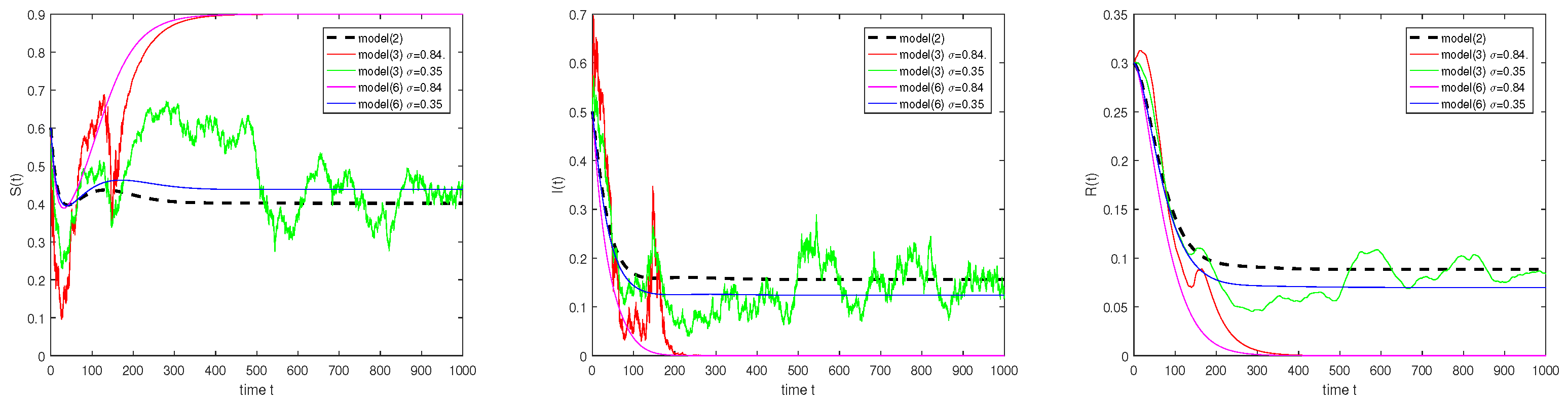
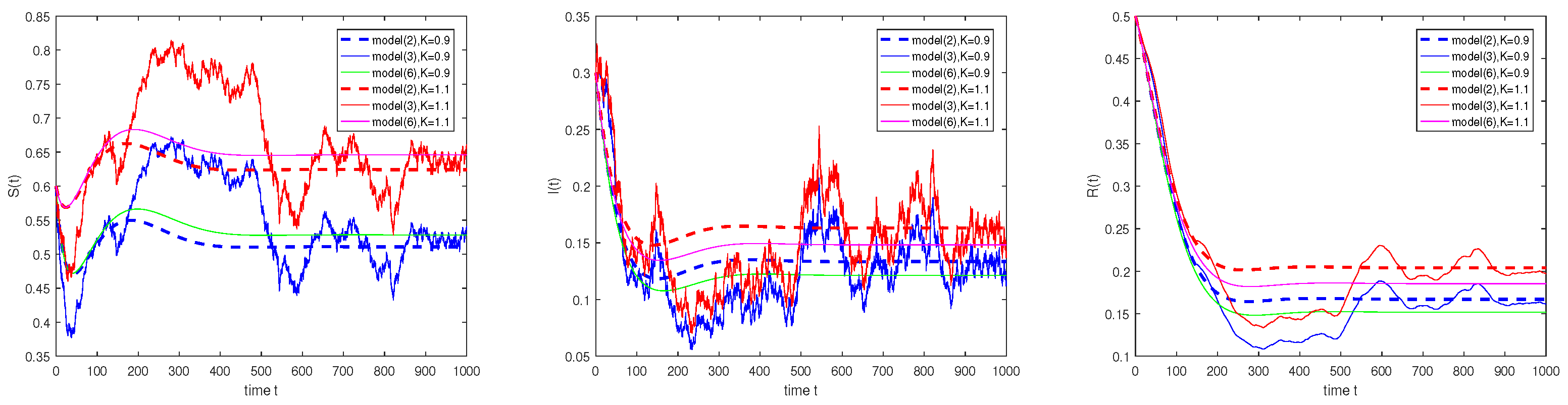
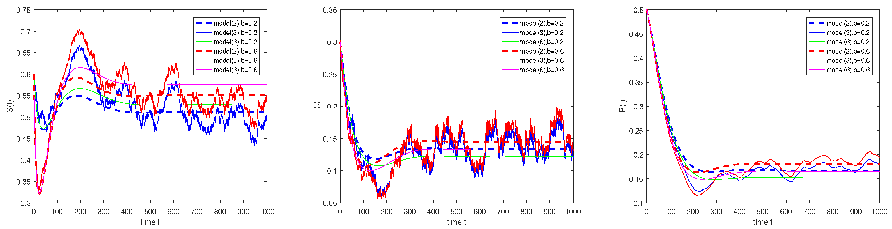
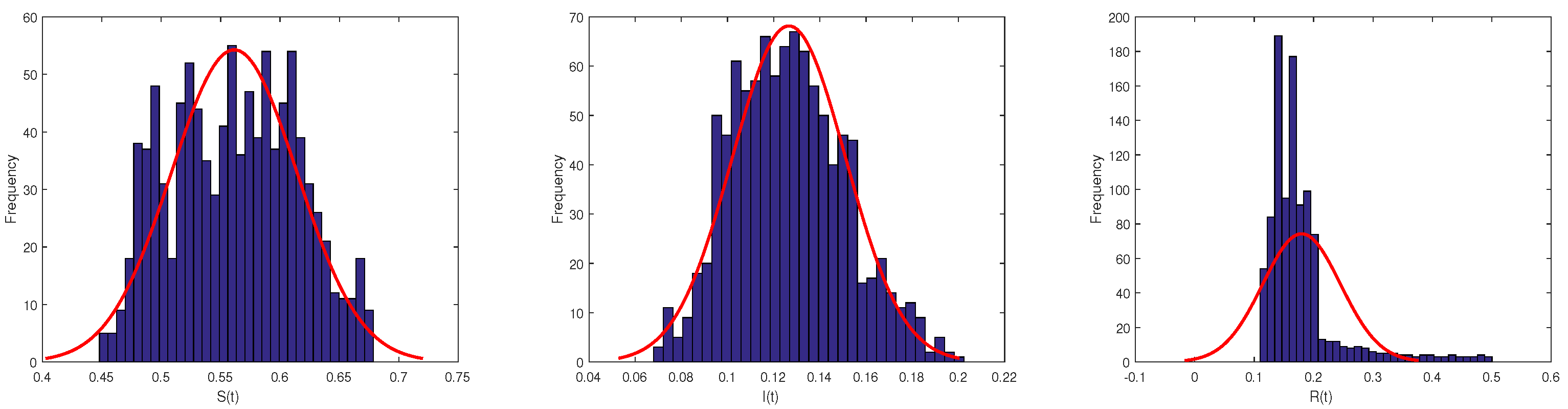
7. Numerical Simulations

In this section, the effect of white noise on model (3) can be determined by the Milstein method in Higham [20]. Thus, we obtain the discretization equations of model (3):

$$\left\{\begin{array}{cc}\hfill S_{k+1}=& S_k+[\left(b-r\frac{S\left(k\right)+I\left(k\right)+R\left(k\right)}{K}\right)\left(S\left(k\right)+I\left(k\right)+R\left(k\right)\right)-\eta f\left(S_k,I_k,R_k\right)+\psi R_k\hfill \\ \hfill & -\mu S_k]\Delta t-f\left(S_k,I_k,R_k\right)\left[\sigma {\xi }_k\sqrt{\Delta t}+\frac{1}{2}{\sigma }^2\left({\xi }_k^2-1\right)\Delta t\right],\hfill \\ \hfill I_{k+1}=& I_k+\left[\eta f\left(S_k,I_k,R_k\right)-(\mu +\varphi +\kappa )I_k\right]\Delta t+f\left(S_k,I_k,R_k\right)\left[\sigma {\xi }_k\sqrt{\Delta t}+\frac{1}{2}{\sigma }^2\left({\xi }_k^2-1\right)\Delta t\right],\hfill \\ \hfill R_{k+1}=& R_k+\left[\varphi I_k-(\mu +\psi )R_k\right]\Delta t,\hfill \end{array}\right.$$

where ${\xi }_k$ are the independent Gaussian random variables that follow the distribution $N(0,1)$ for $k=1,2,\dots ,n$. Here, $f(S,I,R)=SI/N$.

Example 1. 

Assume that $b=0.3$, $r=0.18$, $\psi =0.11$, $K=0.9$, $\eta =0.86$, $\mu =0.12$, $\varphi =0.13$, $\kappa =0.21$, and $\Delta t=0.01$. Obviously, $R_0=1.6087>1$. For model (2), the endemic equilibrium $E^{*}$ is globally asymptotically stable. In model (3), if $\sigma =0.84$, then $R_0^m=0.8417<1$ and ${\sigma }^2-\eta /\partial f(S_0,0,0)/\partial I=-0.0344<0$. Based on Theorem 4 (a), the disease-free equilibrium $E_0$ of model (3) is globally asymptotically stable. It reveals that $S\left(t\right)$ of the models (3) and (6) are close to the environmental capacity K, but $I\left(t\right)$ and $R\left(t\right)$ are close to 0. When $\sigma =0.35$, and $R_0^m=1.4755>1$, the disease is persistent. In addition, the intensity of white noise can suppress the disease outbreak. Figure 1 shows the curves of $\left(S\right(t),I(t),R(t\left)\right)$ under these parameters.

Figure 1. The paths of $S\left(t\right),I\left(t\right)$, and $R\left(t\right)$ under the initial value $\left(S\right(0),I(0),R(0\left)\right)=(0.6,0.5,0.3)$.

Example 2. 

Take the initial value $\left(S\right(0),$ $I\left(0\right),R\left(0\right))=(0.6,0.3,0.5)$, and parameters $\psi =0.11$, $\eta =0.54$, $\mu =0.05$, $\varphi =0.2$, $\kappa =0.09$ and $\sigma =0.2$. The time step size $\Delta t=0.01$. Through the calculation, we have $R_0=1.5882>1$, $R_0^m=1.5294>1$, and $K-B/\mu =0$. Based on Theorem 5, the disease is permanent. Next, we consider the effects of the environmental capacity K and the birth rate b according to two cases:

(i) $K=0.9,1.1$, and $b=0.2$. We observe that $S\left(t\right),I\left(t\right)$, and $R\left(t\right)$ will increase when K increases. Figure 2 illustrates the different evolutions of $S\left(t\right),I\left(t\right)$, and $R\left(t\right)$.

Figure 2. The paths of $S\left(t\right),I\left(t\right)$, and $R\left(t\right)$ under the environmental capacity $K=0.9,1.1$.

(ii) $b=0.6,0.2$, and $K=0.9$. The nonlinear incidence initially becomes larger due to the increase of b, so that $S\left(t\right),I\left(t\right)$, and $R\left(t\right)$ become smaller at the beginning. Moreover, the population slightly increases when the birth rate plays a major role (see Figure 3).

Figure 3. The paths of $S\left(t\right),I\left(t\right)$, and $R\left(t\right)$ under the birth rate $b=0.6,0.2$.

Example 3. 

Take $b=0.3$, $r=0.25$, $K=0.9$, $\eta =0.5$, $\mu =0.05$, $\varphi =0.2$, $\kappa =0.09$, and $\sigma =0.15$. Obviously, $R_0^m=1.4375>1$. From Theorem 6, model (3) has a unique stationary distribution. Figure 4 provides the density functions of $S\left(t\right),I\left(t\right)$, and $R\left(t\right)$ in model (3).

Figure 4. The histograms of $S\left(t\right),I\left(t\right)$, and $R\left(t\right)$ with the initial value $\left(S\right(0),I(0),R(0\left)\right)=(0.6,0.2,0.5)$.

8. Discussion

In this paper, we analyzed the dynamic properties of a stochastic SIRS epidemic model with Logistic birth and nonlinear incidence. Through a Stratonovich SDE, we obtained a new threshold value $R_0^m$ to analyze the stability of model (3). Under the threshold value $R_0^m$, we derived some interesting results, including the global asymptotic stability of the disease-free equilibrium, permanent in the mean of the disease, and the existence of stationary distribution. We observed that environmental noise is a crucial influence in describing the dynamic behaviors of an epidemic. However, there are still some unsolved problems. For example, how to study the relationship of models (6) and (2), as well as (3). It is an exciting issue and will be the subject of our future work.

References

- Beretta, E.; Takeuchi, Y. Convergence results in SIR epidemic models with varying population sizes. Nonlinear Anal. Theory Methods Appl. 1997, 28, 1909–1921. [Google Scholar] [CrossRef]
- Lu, Z.; Chi, X.; Chen, L. The effect of constant and pulse vaccination on SIR epidemic model with horizontal and vertical transmission. Math. Comput. Model. 2002, 36, 1039–1057. [Google Scholar] [CrossRef]
- Zhang, J.; Li, J.; Ma, Z. Global analysis of SIR epidemic models with population size dependent contact rate. J. Eng. Math. 2004, 21, 259–267. [Google Scholar]
- Ma, Z.; Zhou, Y.; Wu, J. Modeling and Dynamics of Infectious Diseases; World Scientific: Singapore, 2009. [Google Scholar]
- Allen, L.J.; Burgin, A.M. Comparison of deterministic and stochastic SIS and SIR models in discrete time. Math. Biosci. 2000, 163, 1–33. [Google Scholar] [CrossRef] [PubMed]
- Gao, L.Q.; Hethcote, H.W. Disease transmission models with density-dependent demographics. J. Math. Biol. 1992, 30, 717–731. [Google Scholar] [CrossRef] [PubMed]
- Korobeinikov, A. Lyapunov functions and global stability for SIR and SIRS epidemiological models with non-linear transmission. Bull. Math. Biol. 2006, 68, 615–626. [Google Scholar] [CrossRef] [PubMed]
- Vargas-De-León, C. Constructions of Lyapunov functions for classic SIS, SIR and SIRS epidemic models with variable population size. Foro-Red-Mat: Rev. Electron Conten. Mat. 2009, 26, 1–12. [Google Scholar]
- Lahrouz, A.; Omari, L.; Kiouach, D. Global analysis of a deterministic and stochastic nonlinear SIRS epidemic model. Nonlinear Anal. 2011, 16, 59–76. [Google Scholar] [CrossRef]
- Li, D.; Cui, J.; Liu, M.; Liu, S. The evolutionary dynamics of stochastic epidemic model with nonlinear incidence rate. Bull. Math. Biol. 2015, 77, 1705–1743. [Google Scholar] [CrossRef] [PubMed]
- Song, Y.; Miao, A.; Zhang, T.; Wang, X.; Liu, J. Extinction and persistence of a stochastic SIRS epidemic model with saturated incidence rate and transfer from infectious to susceptible. Adv. Differ. Equ. 2018, 2018, 1–11. [Google Scholar] [CrossRef]
- Liu, Q.; Jiang, D.; Hayat, T.; Alsaedi, A.; Ahmad, B. A stochastic SIRS epidemic model with logistic growth and general nonlinear incidence rate. Physica A 2020, 551, 124152. [Google Scholar] [CrossRef]
- He, X.; Wei, Y. Dynamics of a Class of Stochastic SIRS Infectious Disease Models With Both Logistic Birth and Markov. Appl. Math. Mech. 2021, 42, 1327–1337. [Google Scholar]
- Mao, X. Stochastic Differential Equations and Applications; Horwood Publishing: Chichester, UK, 2007. [Google Scholar]
- Braumann, C.A. Introduction to Stochastic Differential Equations with Applications to Modelling in Biology and Finance; John Wiley & Sons: Hoboken, NJ, USA, 2019. [Google Scholar]
- Rifhat, R.; Muhammadhaji, A.; Teng, Z. Asymptotic properties of a stochastic SIRS epidemic model with nonlinear incidence and varying population sizes. Dynam. Syst. 2020, 35, 56–80. [Google Scholar] [CrossRef]
- Cai, Y.; Kang, Y.; Wang, W. A stochastic SIRS epidemic model with nonlinear incidence rate. Appl. Math. Comput. 2017, 305, 221–240. [Google Scholar] [CrossRef]
- Khasminskii, R. Stochastic Stability of Differential Equations; Springer Science & Business Media: Berlin/Heidelberg, Germany, 2011. [Google Scholar]
- Liptser, R.S. A strong law of large numbers for local martingales. Stochastics 1980, 3, 217–228. [Google Scholar] [CrossRef]
- Higham, D.J. An algorithmic introduction to numerical simulation of stochastic differential equations. SIAM Rev. 2001, 43, 525–546. [Google Scholar] [CrossRef]
Disclaimer/Publisher’s Note: The statements, opinions and data contained in all publications are solely those of the individual author(s) and contributor(s) and not of MDPI and/or the editor(s). MDPI and/or the editor(s) disclaim responsibility for any injury to people or property resulting from any ideas, methods, instructions or products referred to in the content. |
© 2023 by the authors. Licensee MDPI, Basel, Switzerland. This article is an open access article distributed under the terms and conditions of the Creative Commons Attribution (CC BY) license (https://creativecommons.org/licenses/by/4.0/).