Stochastic Dynamics of a Virus Variant Epidemic Model with Double Inoculations

Abstract

In this paper, we establish a random epidemic model with double vaccination and spontaneous variation of the virus. Firstly, we prove the global existence and uniqueness of positive solutions for a stochastic epidemic model. Secondly, we prove the threshold $R_0^{*}$ can be used to control the stochastic dynamics of the model. If $R_0^{*}<0$, the disease will be extinct with probability 1; whereas if $R_0^{*}>0$, the disease can almost certainly continue to exist, and there is a unique stable distribution. Finally, we give some numerical examples to verify our theoretical results. Most of the existing studies prove the stochastic dynamics of the model by constructing Lyapunov functions. However, the construction of a Lyapunov function of higher-order models is extremely complex, so this method is not applicable to all models. In this paper, we use the definition method suitable for more models to prove the stationary distribution. Most of the stochastic infectious disease models studied now are second-order or third-order, and cannot accurately describe infectious diseases. In order to solve this kind of problem, this paper adopts a higher price five-order model.

1. Introduction

Infectious diseases have become the greatest enemy of human health. When an infectious disease appears and prevails in an area, the primary task is to make every effort to prevent the spread of the disease. Vaccination is one of the important preventive measures. Through vaccination, smallpox was eliminated in the world at the end of the 1970s. This is a great victory for human beings in the fight against infectious diseases, an important milestone in the history of preventive medicine, and a great achievement of vaccination for human beings. In mathematical epidemiology, the control and eradication of infectious diseases are urgent problems, and have greatly attracted the interest of researchers in many fields. Now scholars have proposed and extensively discussed various types of optimizing models and their influencing factors, such as vaccination, time delay, impulse, media reports, etc. [1,2,3,4]. However, as a disease progresses, a virus can mutate as it spreads, allowing the disease to spiral out of control. Cai et al. analyzed the stability of the infectious disease model of virus mutation of inoculation, but only considered the condition that the inoculated individual was completely effective against the virus at a certain stage [5,6]. Baba and Bilgen et al. considered the problem of double-inoculation infectious diseases, which had an adverse effect on the two viruses respectively, but did not consider the conversion between patients infected with the two viruses [7,8]. Therefore, on the basis of the research on the problem of virus mutated infectious disease, considering the situation of two kinds of vaccination for susceptible people, a kind of virus mutated infectious disease model with double vaccination was proposed.

Taking into account the important role of vaccination in preventing the occurrence of infectious diseases, we assume that the first type of vaccinated people are fully immune to the premutation virus and partially resistant to the post mutation virus, whereas the second are fully immune to the postmutation virus and partially resistant to the premutation virus. In addition, the two types of the infected are infectious, and the disease is not fatal before the virus mutation, whereas it is fatal after the virus mutation. Based on the above assumptions, a model was established as follows:

$$\left\{\begin{array}{cc}\hfill \dot{S}(t)& =\mathsf{\Lambda }-{\beta }_{1}S(t)I_1(t)-{\beta }_{2}S(t)I_2(t)-\lambda S(t)\hfill \\ \hfill \dot{V_1}(t)& ={\phi }_{1}S(t)-k_1{I}_2(t)V_1(t)-a{V}_1(t)\hfill \\ \hfill \dot{V_2}(t)& ={\phi }_{2}S(t)-k_2{I}_1(t)V_2(t)-a{V}_2(t)\hfill \\ \hfill \dot{I_1}(t)& ={\beta }_{1}S(t)I_1(t)+k_2{I}_1(t)V_2(t)-{\alpha }_1{I}_1(t)\hfill \\ \hfill \dot{I_2}(t)& ={\beta }_{2}S(t)I_2(t)+k_1{I}_2(t)V_1(t)+\epsilon I_1(t)-{\alpha }_2{I}_2(t)\hfill \\ \hfill \dot{R}(t)& ={\gamma }_1{I}_1(t)+{\gamma }_2{I}_2(t)-aR(t),\hfill \end{array}\right.$$

(1)

where $S(t),V_1(t),V_2(t),I_1(t),I_2(t),$ and $R(t)$, respectively, represent the number at the time t of the susceptible, those vaccinated to the first and to the second types of vaccines, the infected before and after virus mutation, and the recovered. $\mathsf{\Lambda }$ is the input rate of the population. ${\beta }_1$ and ${\beta }_2$ are the infection coefficients, respectively, before and after virus mutation. a is the natural mortality of the population. ${\phi }_1$ and ${\phi }_2$ are the vaccination rates of the first and the second vaccines. $k_1$ and $k_2$ are the infection rates of the infected with the first type of people vaccinated after virus mutation, and the second before virus mutation, respectively. ${\gamma }_1$ and ${\gamma }_2$ are the recovery rates of the infected, respectively, before and after the virus mutation. $\epsilon$ is the ratio of the infected before the virus mutation to the infected after virus mutation in number. $\delta$ is the mortality rate of the infected after virus mutation. In addition, $\lambda :=a+{\phi }_1+{\phi }_2;{\alpha }_1:=a+{\gamma }_1+\epsilon ;{\alpha }_2:=a+{\gamma }_2+\epsilon$.

According to the biological significance of the model, it is assumed that all parameters are positive, and the dynamic behavior of population R does not affect other populations. Thus, the following model is considered:

$$\left\{\begin{array}{cc}\hfill \dot{S}(t)& =\mathsf{\Lambda }-{\beta }_{1}S(t)I_1(t)-{\beta }_{2}S(t)I_2(t)-\lambda S(t)\hfill \\ \hfill \dot{V_1}(t)& ={\phi }_{1}S(t)-k_1{I}_2(t)V_1(t)-a{V}_1(t)\hfill \\ \hfill \dot{V_2}(t)& ={\phi }_{2}S(t)-k_2{I}_1(t)V_2(t)-a{V}_2(t)\hfill \\ \hfill \dot{I_1}(t)& ={\beta }_{1}S(t)I_1(t)+k_2{I}_1(t)V_2(t)-{\alpha }_1{I}_1(t)\hfill \\ \hfill \dot{I_2}(t)& ={\beta }_{2}S(t)I_2(t)+k_1{I}_2(t)V_1(t)+\epsilon I_1(t)-{\alpha }_2{I}_2(t).\hfill \end{array}\right.$$

(2)

Model (2) has a basic reproduction number $R_0$, where

$$R_0=max\{R_1,R_2\},R_1={\displaystyle \frac{{\beta }_1\mathsf{\Lambda }}{{\alpha }_1\lambda }}+{\displaystyle \frac{k_2{\phi }_2\mathsf{\Lambda }}{a{\alpha }_1\lambda }},R_2={\displaystyle \frac{{\beta }_2\mathsf{\Lambda }}{{\alpha }_2\lambda }}+{\displaystyle \frac{k_1{\phi }_1\mathsf{\Lambda }}{a{\alpha }_2\lambda }};$$

it also has a disease-free equilibrium

$$E_0(S_0,V_1^0,V_2^0,0,0)=E_0({\displaystyle \frac{\mathsf{\Lambda }}{\lambda }},{\displaystyle \frac{{\phi }_1\mathsf{\Lambda }}{a\lambda }},{\displaystyle \frac{{\phi }_2\mathsf{\Lambda }}{a\lambda }},0,0).$$

Moreover, when $R_2>0$, model (2) has a boundary equilibrium point

$$E_2(\tilde{S},\widetilde{V_1},\widetilde{V_2},\widetilde{I_1},\widetilde{I_2})=E_2({\displaystyle \frac{\mathsf{\Lambda }}{{\beta }_2\widetilde{I_2}+\lambda }},{\displaystyle \frac{{\phi }_1\mathsf{\Lambda }}{(k_1\widetilde{I_2}+a)({\beta }_2\widetilde{I_2}+\lambda )}},{\displaystyle \frac{{\phi }_2\mathsf{\Lambda }}{a({\beta }_2\widetilde{I_2}+\lambda )}},\widetilde{I_1},\widetilde{I_2}),$$

where the disease will disappear before the virus mutation, and after the virus mutation it will spread; when $I_1^{*}$ and $I_2^{*}>0$, both before and after the virus mutates, model (2) has an endemic disease balance point $E_3(S^{*},V_1^{*},V_2^{*},I_1^{*},I_2^{*})$, where

$$\begin{array}{cc}\hfill & S^{*}={\displaystyle \frac{\mathsf{\Lambda }}{{\beta }_1{I}_1^{*}+{\beta }_2{I}_2^{*}+\lambda }},\hfill \\ \hfill & V_1^{*}={\displaystyle \frac{{\phi }_1\mathsf{\Lambda }}{(k_1{I}_2^{*}+a)({\beta }_1{I}_1^{*}+{\beta }_2{I}_2^{*}+\lambda )}},\hfill \\ \hfill & V_2^{*}={\displaystyle \frac{{\phi }_2\mathsf{\Lambda }}{(k_2{I}_1^{*}+a)({\beta }_1{I}_1^{*}+{\beta }_2{I}_2^{*}+\lambda )}}.\hfill \end{array}$$

On the other hand, environmental change has a key impact on the development of epidemics [9]. For disease transmission, because of the unpredictability of human contact, the growth and spread of epidemics are essentially random, so population numbers are constantly disturbed [10,11]. Therefore, in epidemic dynamics, stochastic differential equation $(SDE)$ models may be a more appropriate approach to modeling epidemics in many situations. Many real stochastic epidemic models can be derived based on their deterministic formulas [9,12,13,14,15,16,17,18,19,20,21,22,23]. Assuming that the coefficients of model (2) are affected by random noise that can be represented by Brownian motion, model (2) becomes:

$$\left\{\begin{array}{cc}\hfill dS(t)& =(\mathsf{\Lambda }-{\beta }_{1}S{I}_1-{\beta }_{2}S{I}_2-\lambda S)dt+{\sigma }_{1}Sd{B}_1(t)\hfill \\ \hfill d{V}_1(t)& =({\phi }_{1}S-k_1{I}_2{V}_1-a{V}_1)dt+{\sigma }_2{V}_{1}d{B}_2(t)\hfill \\ \hfill d{V}_2(t)& =({\phi }_{2}S-k_2{I}_1{V}_2-a{V}_2)dt+{\sigma }_3{V}_{2}d{B}_3(t)\hfill \\ \hfill d{I}_1(t)& =({\beta }_{1}S{I}_1+k_2{I}_1{V}_2-{\alpha }_1{I}_1)dt+{\sigma }_4{I}_{1}d{B}_4(t)\hfill \\ \hfill d{I}_2(t)& =({\beta }_{2}S{I}_2+k_1{I}_2{V}_1+\epsilon I_1-{\alpha }_2{I}_2)dt+{\sigma }_5{I}_{2}d{B}_5(t),\hfill \end{array}\right.$$

(3)

where ${\sigma }_i(i=1,2,3,4,5)$ represents the intensities of the white noises, and $B_i(t)(i=1,2,3,4,5)$ are mutually independent standard Brownian motions. However, the groups $S,V_1,V_2,I_1,$ and $I_2$ are usually subject to the same random factors such as temperature, humidity, etc., in reality. As a result, it is more reasonable to assume that the five classes of random perturbance noises are uncorrelated. If we set $B_i(t)=B(t)(i=1,2,3,4,5)$, then model (3) becomes:

$$\left\{\begin{array}{cc}\hfill dS(t)& =(\mathsf{\Lambda }-{\beta }_{1}S{I}_1-{\beta }_{2}S{I}_2-\lambda S)dt+{\sigma }_{1}SdB(t)\hfill \\ \hfill d{V}_1(t)& =({\phi }_{1}S-k_1{I}_2{V}_1-a{V}_1)dt+{\sigma }_2{V}_{1}dB(t)\hfill \\ \hfill d{V}_2(t)& =({\phi }_{2}S-k_2{I}_1{V}_2-a{V}_2)dt+{\sigma }_3{V}_{2}dB(t)\hfill \\ \hfill d{I}_1(t)& =({\beta }_{1}S{I}_1+k_2{I}_1{V}_2-{\alpha }_1{I}_1)dt+{\sigma }_4{I}_{1}dB(t)\hfill \\ \hfill d{I}_2(t)& =({\beta }_{2}S{I}_2+k_1{I}_2{V}_1+\epsilon I_1-{\alpha }_2{I}_2)dt+{\sigma }_5{I}_{2}dB(t).\hfill \end{array}\right.$$

(4)

Let $(\mathsf{\Omega },\mathcal{F},{\{{\mathcal{F}}_t\}}_{t\ge 0},\mathbb{P})$ be a complete probability space with the filtration ${\{{\mathcal{F}}_t\}}_{t\ge 0}$ satisfying the usual condition (i.e., ${\{{\mathcal{F}}_t\}}_{t\ge 0}$ is increasing and right continuous whereas ${\mathcal{F}}_0$ contains all $\mathbb{P}$-null sets). Throughout this paper, $a\wedge b:=min\{a,b\}$, $a\vee b:=max\{a,b\}$ and $R_{+}^{5,\circ }:=\{(u,v,w,x,y):u,v,w,x,y>0\}$ are denoted.

First, we prove the global existence and uniqueness of the positive solution of model (4). Similar to a deterministic model, we introduce a threshold value $R_0^{*}$, able to be calculated from the coefficients. We show that if $R_0^{*}<0$, $I(t),I(t)=I_1(t)+I_2(t)$ will be extinct with probability 1, and $S(t),V_1(t),V_2(t)$ will weakly converge to their unique invariant probability measures ${\mu }_1^{*},{\mu }_2^{*},{\mu }_3^{*}$, respectively. If $R_0^{*}>0$, then coexistence occurs, and all positive solutions of model (4) are converged to the unique variational probability measure ${\mu }^{*}$ in the total variational norm.

Most of the existing studies use the method of constructing the Lyapunov function to prove the existence of the stationary distribution of the solution of model (4). However, this method is not applicable to all models. In this paper, the definition method applicable to more models is used to prove the stationary distribution [24,25,26,27]. Moreover, most of the stochastic infectious disease models studied now are second order or third order. Therefore, in order to depict infectious diseases more accurately, we have established a fifth-order model–a double inoculation and random infectious disease model of spontaneous virus mutation, considering two kinds of vaccination for susceptible people on the basis of the research on infectious diseases of virus mutation.

The main structure of this paper is as follows: In Section 2 we prove the global existence and uniqueness of the positive solution of model (4). In Section 3 and Section 4, we are devoted to the proof of extinction and coexistence, respectively. In Section 5, we provide an example to support our findings. In Section 6, the main results are discussed and summarized briefly.

2. Existence and Uniqueness of the Global Solutions

Theorem 1.

For any given value $(S(0),V_1(0),V_2(0),I_1(0),I_2(0))$, there is a unique solution $(S(t),V_1(t),V_2(t),I_1(t),I_2(t))$ to model (4) on $t\ge 0$ and the solution will remain in $R_{+}^{5,\circ }$ with probability 1, i.e., $(S(t),V_1(t),V_2(t),I_1(t),I_2(t))$ in $R_{+}^{5,\circ }$ for all $t\ge 0$ almost surely.

Proof of Theorem 1.

Since the coefficients of model (4) satisfy local Lipschitz and linear growth conditions, it can be seen from the existence and uniqueness theorem of solutions of stochastic differential equations that for any $(S(0),V_1(0),V_2(0),I_1(0),I_2(0))\in R_{+}^{5,\circ }$, model (4) has a locally unique solution $(S(t),V_1(t),V_2(t),I_1(t),I_2(t))$. To prove the global nature of the solution, we only need to prove that ${\tau }_e=+\infty$, where ${\tau }_e$ is the explosion time.

Let $k_0>0$ be a sufficiently large positive number, so that for each $t\ge 0$, $S(t)$, $V_1(t)$, $V_2(t)$, $I_1(t)$, $I_2(t)$ fall in the interval $[\frac{1}{k_0},k_0]$. For each integer $k>k_0$, define the stop time ${\tau }_e$ as follows:

$$\begin{array}{cc}\hfill & {\tau }_k=inf\{t\in \left[0,{\tau }_e\right]:S(t)\notin ({\displaystyle \frac{1}{k}},k),or{V}_1(t)\notin ({\displaystyle \frac{1}{k}},k),or{V}_2(t)\notin ({\displaystyle \frac{1}{k}},k),or{I}_1(t)\notin ({\displaystyle \frac{1}{k}},k),or{I}_2(t)\notin ({\displaystyle \frac{1}{k}},k)\},\hfill \end{array}$$

where $inf\varnothing =\infty$. Obviously, when $k\to \infty$, ${\tau }_k$ increases monotonously.

Let ${\tau }_{\infty }={lim}_{k\to +\infty }{\tau }_k$, then ${\tau }_{\infty }\le {\tau }_e$. So we just have to prove ${\tau }_{\infty }=\infty$. Supposing that ${\tau }_{\infty }\ne \infty$, then there are constants $T>0$ and ${\epsilon }_1\in (0,1)$ such that $P\{{\tau }_{\infty }\le T\}>{\epsilon }_1$. Further, there is an integer $k_1\le k_0$ that makes

$$P\{{\tau }_k\le T\}\ge {\epsilon }_{1}forallk\ge k_1.$$

(5)

Define $C^5$ function: $V:R_{+}^{5,\circ }\to R_{+}$ by $V(N(t))=N(t)-1-lnN(t)$, where $N(t):=S(t)+V_1(t)+V_2(t)+I_1(t)+I_2(t)$. Obviously, function $V(N(t))$ is a non-negative function. If $(S(t),V_1(t),V_2(t),I_1(t),I_2(t))\in R_{+}^{5,\circ }$, according to $It{\widehat{o}}^{\prime }s$ formula, there is a positive number $G:=\mathsf{\Lambda }+a+{\gamma }_1+{\gamma }_2+\delta +{\displaystyle \frac{1}{2}}({\sigma }_1^2+{\sigma }_2^2+{\sigma }_3^2+{\sigma }_4^2+{\sigma }_5^2)$, so that

$$\begin{array}{cc}\hfill dV& =LVdt+(1-{\displaystyle \frac{1}{N}})({\sigma }_{1}S+{\sigma }_2{V}_1+{\sigma }_3{V}_2+{\sigma }_4{I}_1+{\sigma }_5{I}_2)dB(t),\hfill \\ \hfill LV& =(1-{\displaystyle \frac{1}{N}})[\mathsf{\Lambda }-aN-{\gamma }_1{I}_1-({\gamma }_2+\delta )I_2]+{\displaystyle \frac{1}{2N^2}}({\sigma }_1^2{S}^2+{\sigma }_2^2{V}_1^2+{\sigma }_3^2{V}_2^2+{\sigma }_4^2{I}_1^2+{\sigma }_5^2{I}_2^2)\hfill \\ \hfill & =\mathsf{\Lambda }-aN-{\gamma }_1{I}_1-({\gamma }_2+\delta )I_2-{\displaystyle \frac{\mathsf{\Lambda }}{N}}+a+{\displaystyle \frac{{\gamma }_1{I}_1}{N}}+{\displaystyle \frac{({\gamma }_2+\delta )I_2}{N}}\hfill \\ \hfill & +{\displaystyle \frac{1}{2N^2}}({\sigma }_1^2{S}^2+{\sigma }_2^2{V}_1^2+{\sigma }_3^2{V}_2^2+{\sigma }_4^2{I}_1^2+{\sigma }_5^2{I}_2^2)\hfill \\ \hfill & \le \mathsf{\Lambda }+a+{\gamma }_1+{\gamma }_2+\delta +{\displaystyle \frac{1}{2}}({\sigma }_1^2+{\sigma }_2^2+{\sigma }_3^2+{\sigma }_4^2+{\sigma }_5^2)\hfill \\ \hfill & :=G,\hfill \\ \hfill dV& \le Gdt+(1-{\displaystyle \frac{1}{N}})({\sigma }_{1}S+{\sigma }_2{V}_1+{\sigma }_3{V}_2+{\sigma }_4{I}_1+{\sigma }_5{I}_2)dB(t).\hfill \end{array}$$

Integrate both sides of the above inequality from 0 to ${\tau }_k\wedge T$ at the same time, we get

$$\begin{array}{c}\hfill {\int }_0^{{\tau }_k\wedge T}dV\le {\int }_0^{{\tau }_k\wedge T}Gdt+{\int }_0^{{\tau }_k\wedge T}(1-{\displaystyle \frac{1}{N}})({\sigma }_{1}S+{\sigma }_2{V}_1+{\sigma }_3{V}_2+{\sigma }_4{I}_1+{\sigma }_5{I}_2)dB(t),\end{array}$$

moreover, then we take the expectation, and obtain

$$\begin{array}{c}\hfill EV(N({\tau }_k\wedge T))\le V(N(0))+GE({\tau }_k\wedge T)\le V(N(0))+GT.\end{array}$$

(6)

Set ${\mathsf{\Omega }}_k=\{{\tau }_k\le T\}$ for $k\ge k_1$ and by (5), we have $P({\mathsf{\Omega }}_k)\ge {\epsilon }_1$. Noting that for every $\omega \in {\mathsf{\Omega }}_k$, there is $S({\tau }_k,\omega )$ or $V_1({\tau }_k,\omega )$ or $V_2({\tau }_k,\omega )$ or $I_1({\tau }_k,\omega )$ or $I_2({\tau }_k,\omega )$, being equal to either k or $\frac{1}{k}$, and hence

$$V((N({\tau }_k,\omega ))\ge min\{k-1-lnk,{\displaystyle \frac{1}{k}}-1+lnk\}.$$

It then follows from (6) that

$$V(N(0))+GT\ge E[1_{{\mathsf{\Omega }}_k}(\omega )V(N(\omega ))]\ge {\epsilon }_{1}min\{k-1-lnk,{\displaystyle \frac{1}{k}}-1+lnk\},$$

where $1_{{\mathsf{\Omega }}_k}$ is the indicator function of ${\mathsf{\Omega }}_k$. Letting $k\to \infty$, we obtain the following contradiction:

$$\infty >V(N(0))+GT=\infty .$$

So we must have ${\tau }_{\infty }=\infty$ a.s. This completes the proof of Theorem 1. □

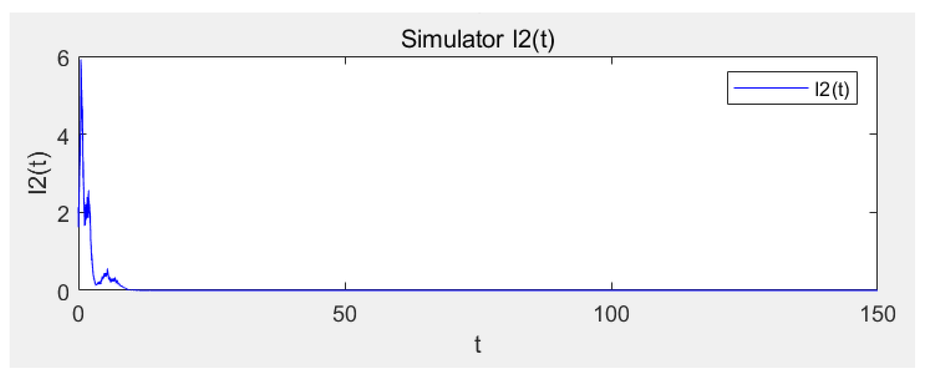
3. Extinction of Disease

For the infectious disease model, we always care about whether the disease will disappear. In this section, we first define a threshold value $R_0^{*}$, and the stochastic extinction of the disease when $R_0^{*}<0$ is then proved in the model (4).

To obtain further properties of the solution, we case on the boundary of the first equation of model (4):

$$d\overline{S}(t)=[\mathsf{\Lambda }-\lambda \overline{S}(t)]dt+{\sigma }_1\overline{S}(t)dB(t)$$

(7)

so we have,

$${\displaystyle \frac{1}{t}}{\int }_0^t\overline{S}(\tau )d\tau ={\displaystyle \frac{\overline{S}(0)-\overline{S}(t)}{\lambda t}}+{\displaystyle \frac{\mathsf{\Lambda }}{\lambda }}+{\displaystyle \frac{{\sigma }_1}{\lambda t}}{\int }_0^t\overline{S}(\tau )dB(\tau ).$$

For the given initial value u, let $\overline{S}(t)$ be the solution to model (7). According to the comparison theorem, $S_{u,v,w,x,y}\le \overline{S}(t)$$\forall t\ge 0$. By solving the Fokker–Planck equation, the process $\overline{S}(t)$ has unique stationary distribution with density $f_1^{*}(x)$, and by the strong law of large numbers, we have

$$\underset{t\to \infty }{lim}{\displaystyle \frac{1}{t}}{\int }_0^t\overline{S}(\tau )d\tau ={\int }_0^{\infty }x{f}_1^{*}(x)dx={\displaystyle \frac{\mathsf{\Lambda }}{\lambda }}.$$

(8)

For other equations of model (4), we use the same method to obtain:

$$d{\overline{V}}_1(t)=[{\phi }_1\overline{S}(t)-a{\overline{V}}_1(t)]dt+{\sigma }_2{\overline{V}}_1(t)dB(t),$$

we have

$$\underset{t\to \infty }{lim}{\displaystyle \frac{1}{t}}{\int }_0^t{\overline{V}}_1(\tau )d\tau ={\int }_0^{\infty }x{f}_2^{*}(x)dx={\displaystyle \frac{{\phi }_1\mathsf{\Lambda }}{a\lambda }},$$

(9)

then similarly

$$d{\overline{V}}_2(t)=[{\phi }_2\overline{S}(t)-a{\overline{V}}_2(t)]dt+{\sigma }_3{\overline{V}}_2(t)dB(t),$$

therefore

$$\underset{t\to \infty }{lim}{\displaystyle \frac{1}{t}}{\int }_0^t{\overline{V}}_2(\tau )d\tau ={\int }_0^{\infty }x{f}_3^{*}(x)dx={\displaystyle \frac{{\phi }_2\mathsf{\Lambda }}{a\lambda }},$$

(10)

where $f_2^{*}(x),f_3^{*}(x)$ have the same definition as above.

To proceed, we define the threshold as follows:

$$R_0^{*}={\displaystyle \frac{({\beta }_1+{\beta }_2)\mathsf{\Lambda }}{\lambda }}+{\displaystyle \frac{k_1{\phi }_1\mathsf{\Lambda }}{a\lambda }}+{\displaystyle \frac{k_2{\phi }_2\mathsf{\Lambda }}{a\lambda }}+\epsilon -\alpha ,$$

where $\alpha ={\alpha }_1\wedge {\alpha }_2$.

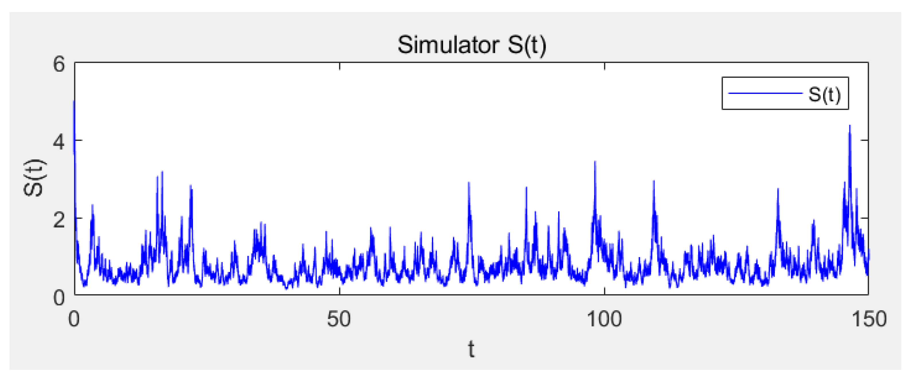
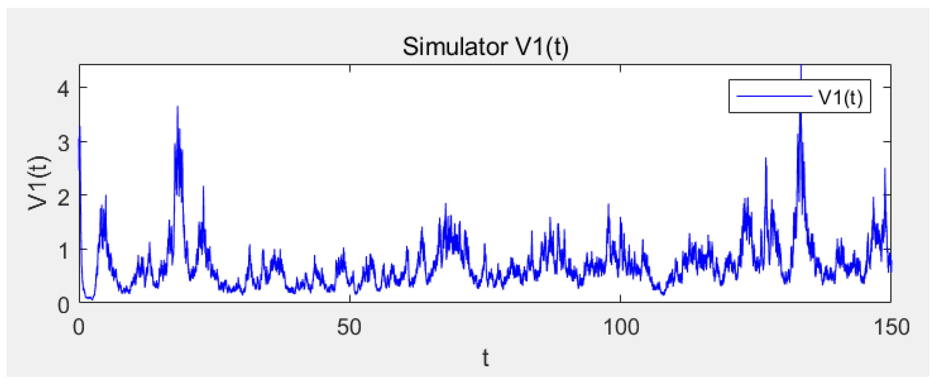
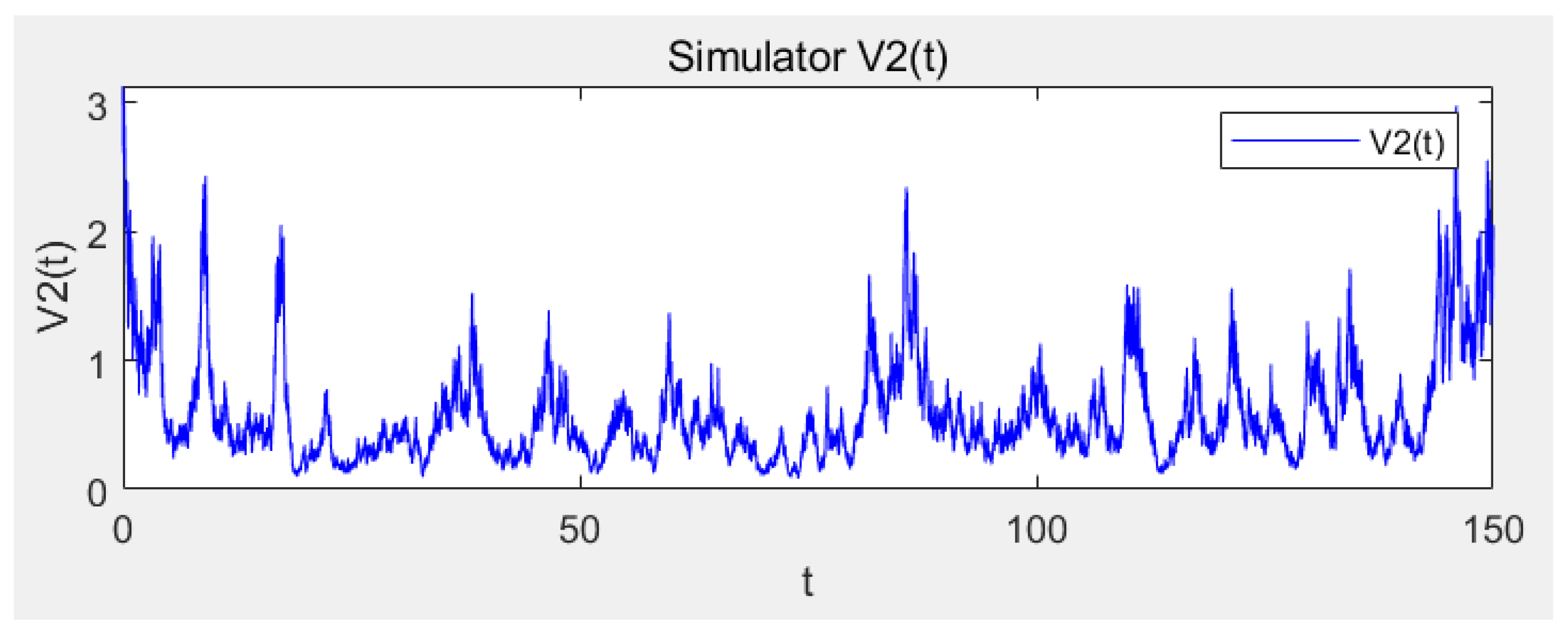
Theorem 2.

If $R_0^{*}<0$, then for any initial value $(S(0),V_1(0),V_2(0),I_1(0),I_2(0))=(u,v,w,x,y)$$\in R_{+}^{5,\circ }$, ${lim\; sup}_{t\to \infty }\frac{ln{I}_{u,v,w,x,y}(t)}{t}\le R_0^{*}$ a.s., and the distribution of $Su,v,w,x,y(t),V_{1_{u,v,w,x,y}}(t)$, $V_{2_{u,v,w,x,y}}(t)$ converge weakly to the unique invariant probability measures ${\mu }_1^{*},{\mu }_2^{*},{\mu }_3^{*}$ with the densities $f_1^{*},f_2^{*},f_3^{*}$, respectively.

Proof of Theorem 2.

Considering a Lyapunov function $I(t)$, defined by $I(t)=I_1(t)+I_2(t)$. Applying $It{\widehat{o}}^{\prime }s$ formula to $I(t)$, we have

$$\begin{array}{cc}\hfill dlnI(t)& =[{\displaystyle \frac{1}{I(t)}}({\beta }_{1}S(t)I_1(t)+k_2{I}_1(t)V_2(t)-{\alpha }_1{I}_1(t)+{\beta }_{2}S(t)I_2(t)+k_1{I}_2(t)V_1(t)\hfill \\ \hfill & +\epsilon I_1(t)-{\alpha }_2{I}_2(t))-{\displaystyle \frac{{\sigma }_4^2{I}_1{(t)}^2+{\sigma }_5^2{I}_2{(t)}^2}{2I^2(t)}}]dt+{\displaystyle \frac{{\sigma }_4{I}_1(t)+{\sigma }_5{I}_2(t)}{I(t)}}dB(t)\hfill \\ \hfill & \le [({\beta }_1+{\beta }_2)S(t)+{\displaystyle \frac{k_2{I}_1(t)}{I(t)}}{V}_2(t)+{\displaystyle \frac{k_1{I}_2(t)}{I(t)}}{V}_1(t)+\epsilon {\displaystyle \frac{I_1(t)}{I(t)}}-\alpha ]dt+{\displaystyle \frac{{\sigma }_4{I}_1(t)+{\sigma }_5{I}_2(t)}{I(t)}}dB(t)\hfill \\ \hfill & \le [({\beta }_1+{\beta }_2)\overline{S}(t)+k_1{\overline{V}}_1(t)+k_2{\overline{V}}_2(t)+\epsilon -\alpha ]dt+({\sigma }_4+{\sigma }_5)dB(t),\hfill \end{array}$$

where $\alpha ={\alpha }_1\wedge {\alpha }_2$.

Then integral from 0 to t at both ends of inequality

$$\begin{array}{cc}\hfill lnI(t)-lnI(0)& \le ({\beta }_1+{\beta }_2){\int }_0^t\overline{S}(\tau )d\tau +k_1{\int }_0^t{\overline{V}}_1(\tau )d\tau +k_2{\int }_0^t{\overline{V}}_2(\tau )d\tau \hfill \\ \hfill & +(\epsilon -\alpha )t+({\sigma }_4+{\sigma }_5){\int }_0^{t}dB(\tau ).\hfill \end{array}$$

(11)

It finally follows from (11) by dividing t on the both sides and let $t\to \infty$ that,

$$\underset{t\to \infty }{lim\; sup}{\displaystyle \frac{1}{t}}lnI(t)={\displaystyle \frac{({\beta }_1+{\beta }_2)\mathsf{\Lambda }}{\lambda }}+{\displaystyle \frac{k_1{\phi }_1\mathsf{\Lambda }}{a\lambda }}+{\displaystyle \frac{k_2{\phi }_2\mathsf{\Lambda }}{a\lambda }}+\epsilon -\alpha =R_0^{*}<0.$$

(12)

Hence, $I(t)$ converges almost surely to 0 at an exponential rate.

For any ${\epsilon }_1>0$, it follows from (12) that there exists $t_0>0$ such that $P({\mathsf{\Omega }}_{{\epsilon }_1})>1-{\epsilon }_1$ where

$${\mathsf{\Omega }}_{{\epsilon }_1}=\{lnI(t)\le R_0^{*}t\}=\{I(t)\le e^{R_0^{*}t},\forall t\ge t_0\}.$$

Case 1.

$S_{u,v,w,x,y}(t)$ converges weakly to the unique invariant probability measure ${\mu }_1^{*}$ with the density $f_1^{*}$.

We can choose that $t_0$ satisfying $-\frac{2\beta }{R_0^{*}}exp\{R_0^{*}\}<{\epsilon }_1$. Let $\overline{S}(t)$ be the solution of (7). Supposing $\overline{S}(t_0)=S(t_0)$, then we can obtain $P\{S_{u,v,w,x,y}(t)\le \overline{S}(t)\}=1$ by the comparison theorem. In view of the $It{\widehat{o}}^{\prime }s$ formula, for almost all $\varpi \in {\mathsf{\Omega }}_{{\epsilon }_1}$ we have

$$\begin{array}{cc}\hfill 0\le ln\overline{S}(t)-lnS(t)& =\mathsf{\Lambda }{\int }_{t_0}^t({\displaystyle \frac{1}{\overline{S}(\tau )}}-{\displaystyle \frac{1}{S(\tau )}})d\tau +{\int }_{t_0}^t({\beta }_1{I}_1(\tau )+{\beta }_2{I}_2(\tau ))d\tau \hfill \\ \hfill & \le \beta {\int }_{t_0}^{t}I(\tau )d(\tau )\le \beta {\int }_{t_0}^t{e}^{R_0^{*}\tau }d\tau =-{\displaystyle \frac{\beta }{R_0^{*}}}(e^{R_0^{*}{t}_0}-e^{R_0^{*}t})<{\epsilon }_1,\hfill \end{array}$$

where $\beta ={\beta }_1\vee {\beta }_2$. As a result, for any $t\ge t_0$ we have

$$P\{|lnS(t)-ln\overline{S}(t)|\le {\epsilon }_1\}>1-{\epsilon }_1\iff P\{|lnS(t)-ln\overline{S}(t)|>{\epsilon }_1\}<{\epsilon }_1.$$

(13)

Now let us make an equivalent statement, that is, the distribution of $lnS(t)$ is weakly convergent to ${\nu }_1^{*}$ is equivalent to the distribution of $S(t)$ is weakly convergent to ${\mu }_1^{*}$. By the Portmanteau theorem, it is sufficient to prove that for any $g(·):R\to R$ satisfying $|g(x)-g(y)|\le |x-y|$ and $\left|g(x)\right|<1$$\forall x,y\in R$, we have

$$Eg(ln{S}_{u,v,w,x,y}(t))\to {\overline{g}}_1:={\int }_{R}g(x){\nu }_1^{*}(dx)={\int }_0^{\infty }g(lnx){\mu }_1^{*}(dx).$$

Because the diffusion of model (4) is non-degenerate, the distribution of $\overline{S}$ converges weakly to ${\mu }_1^{*}$ as $t\to \infty$. Therefore

$$\underset{t\to \infty }{lim}Eg(ln\overline{S}(t))={\overline{g}}_1,$$

(14)

such that

$$\begin{array}{cc}\hfill |E{g}_1(lnS(t))-{\overline{g}}_1|& =|Eg(lnS(t))-E{g}_1(ln\overline{S}(t))+E{g}_1(ln\overline{S}(t))-{\overline{g}}_1|\hfill \\ \hfill & \le E|lnS(t)-ln\overline{S}(t)|+E|g_1(ln\overline{S}(t))-{\overline{g}}_1|\hfill \\ \hfill & \le \{|lnS(t)-ln\overline{S}(t)|<{\epsilon }_1\}P\{|lnS(t)-ln\overline{S}(t)|<{\epsilon }_1\}\hfill \\ \hfill & +\{|lnS(t)-ln\overline{S}(t)|\ge {\epsilon }_1\}P\{|lnS(t)-ln\overline{S}(t)|>{\epsilon }_1\}\hfill \\ \hfill & \le {\epsilon }_{1}P\{|lnS(t)-ln\overline{S}(t)|<{\epsilon }_1\}+2{\epsilon }_{1}P\{|lnS(t)-ln\overline{S}(t)|>{\epsilon }_1\}.\hfill \end{array}$$

(15)

Applying (13) and (14) to (15), we can obtain

$$\underset{t\to \infty }{lim\; sup}|Eg(lnS(t))-{\overline{g}}_1|\le 3{\epsilon }_1.$$

Case 2.

$V_{1u,v,w,x,y}(t)$ converges weakly to the unique invariant probability measure ${\mu }_2^{*}$ with the density $f_2^{*}$.

Similar to Case 1, we can choose $t_0$ satisfying $-\frac{2k_1}{R_0^{*}}exp\{R_0^{*}\}<{\epsilon }_1$. Then, we can get

$$\begin{array}{cc}\hfill ln{\overline{V}}_1(t)-ln{V}_1(t)& ={\phi }_1{\int }_{t_0}^t({\displaystyle \frac{\overline{S}(\tau )}{{\overline{V}}_1(\tau )}}-{\displaystyle \frac{S(\tau )}{V_1(\tau )}})d\tau +k_1{\int }_{t_0}^t{I}_2(\tau )d\tau \le k_1{\int }_{t_0}^{t}I(\tau )d(\tau )\hfill \\ \hfill & \le k_1{\int }_{t_0}^t{e}^{R_0^{*}\tau }d\tau =-{\displaystyle \frac{k_1}{R_0^{*}}}(e^{R_0^{*}{t}_0}-e^{R_0^{*}t})<{\epsilon }_1.\hfill \end{array}$$

As a result, for any $t\ge t_0$ we have

$$P\{|ln{V}_1(t)-ln{\overline{V}}_1(t)|\le {\epsilon }_1\}>1-{\epsilon }_1\iff P\{|ln{V}_1(t)-ln\overline{V_1}(t)|>{\epsilon }_1\}<{\epsilon }_1,$$

(16)

then we have

$$Eg(ln{V}_{1u,v,w,x,y}(t))\to {\overline{g}}_2:={\int }_{R}g(x){\nu }_2^{*}(dx)={\int }_0^{\infty }g(lnx){\mu }_2^{*}(dx).$$

Thus

$$\underset{t\to \infty }{lim}Eg(ln{\overline{V}}_{1v}(t))={\overline{g}}_2,$$

(17)

such that

$$\begin{array}{cc}\hfill |E{g}_1(lnS(t))-{\overline{g}}_1|& =|Eg(lnS(t))-E{g}_1(ln\overline{S}(t))+E{g}_1(ln\overline{S}(t))-{\overline{g}}_1|\hfill \\ \hfill & \le {\epsilon }_{1}P\{|lnS(t)-ln\overline{S}(t)|<{\epsilon }_1\}+2{\epsilon }_{1}P\{|lnS(t)-ln\overline{S}(t)|>{\epsilon }_1\}.\hfill \end{array}$$

(18)

Applying (16) and (17) to (18), we can obtain

$$\underset{t\to \infty }{lim\; sup}|Eg(ln{V}_{1u,v,w,x,y}(t))-{\overline{g}}_2|\le 3{\epsilon }_1.$$

Case 3.

$V_{2u,v,w,x,y}(t)$ converges weakly to the unique invariant probability measure ${\mu }_3^{*}$ with the density $f_3^{*}$.

The proof method is the same as above. Since ${\epsilon }_1$ is taken arbitrarily, we obtain the desired conclusion. The proof is completed. □

4. Stationary Distribution

Now we focus on the case $R_0^{*}>0$. Let $P(t,(u,v,w,x,y),·)$ be the transition probability of $(S_{u,v,w,x,y}(t),V_{1u,v,w,x,y}(t),V_{2u,v,w,x,y}(t),I_{1u,v,w,x,y}(t),I_{2u,v,w,x,y}(t))$. Because the diffusion of model (4) is degenerate, i.e., $B_1(t)=B_2(t)=B_3(t)=B_4(t)=B_5(t)=B(t)$, we have to change the model to Stratonovich’s form in order to obtain properties of $P(t,(u,v,w,x,y),·)$,

$$\left\{\begin{array}{cc}\hfill dS(t)& =(\mathsf{\Lambda }-c_{1}S(t)-{\beta }_{1}S(t)I_1(t)-{\beta }_{2}S(t)I_2(t))dt+{\sigma }_{1}S(t)\circ dB(t)\hfill \\ \hfill d{V}_1(t)& =(-c_2{V}_1(t)+{\phi }_{1}S(t)-k_1{I}_2(t)V_1(t))dt+{\sigma }_2{V}_1(t)\circ dB(t)\hfill \\ \hfill d{V}_2(t)& =(-c_3{V}_2(t)+{\phi }_{2}S(t)-k_2{I}_1(t)V_2(t))dt+{\sigma }_3{V}_2(t)\circ dB(t)\hfill \\ \hfill d{I}_1(t)& =(-c_4{I}_1(t)+{\beta }_{1}S(t)I_1(t)+k_2{I}_1(t)V_2(t))dt+{\sigma }_4{I}_1(t)\circ dB(t)\hfill \\ \hfill d{I}_2(t)& =(-c_5{I}_2(t)+{\beta }_{2}S(t)I_2(t)+k_1{I}_2(t)V_1(t)+\epsilon I_1(t))dt+{\sigma }_5{I}_2(t)\circ dB(t),\hfill \end{array}\right.$$

where

$$c_1=\lambda +{\displaystyle \frac{{\sigma }_1^2}{2}};c_2=a+{\displaystyle \frac{{\sigma }_2^2}{2}};c_3=a+{\displaystyle \frac{{\sigma }_3^2}{2}};c_4={\alpha }_1+{\displaystyle \frac{{\sigma }_4^2}{2}};c_5={\alpha }_2+{\displaystyle \frac{{\sigma }_5^2}{2}}.$$

Let

$$A(u,v,w,x,y)=\left(\begin{array}{c}\mathsf{\Lambda }-c_{1}u-{\beta }_{1}ux-{\beta }_{2}uy\\ -c_{2}v+{\phi }_{1}u-k_{1}vy\\ -c_{3}w+{\phi }_{2}u-k_{2}wx\\ -c_{4}x+{\beta }_{1}ux+k_{2}wx\\ -c_{5}y+{\beta }_{2}uy+k_{1}vy+\epsilon x\end{array}\right),B=\left(\begin{array}{c}{\sigma }_{1}u\\ {\sigma }_{2}v\\ {\sigma }_{3}w\\ {\sigma }_{4}x\\ {\sigma }_{5}y\end{array}\right),$$

to proceed, we first recall the notion of Lie bracket. If $X(a_1,a_2,\cdots ,a_n)={(X_1,X_2,\cdots ,X_n)}^{\top }$ and $Y(a_1,a_2,\cdots ,a_n)={(Y_1,Y_2,\cdots ,Y_n)}^{\top }$ are two vector fields on $R^n$ then the Lie bracket $[X,Y]$ is a vector field given by

$${[X,Y]}_i(a_1,a_2,\cdots ,a_n)=\sum _{j=1}^n(X_j{\displaystyle \frac{\partial Y_i}{\partial x_i}}(a_1,a_2,\cdots ,a_n)-Y_j{\displaystyle \frac{\partial X_i}{\partial x_i}}(a_1,a_2,\cdots ,a_n)),$$

where $i=1,2,\cdots ,n.$

Using $\mathcal{L}(u,v,w,x,y)$ to represent the Lie algebra generated by $A(u,v,w,x,y)$, $B(u,v,w,x,y)$ and ${\mathcal{L}}_0(u,v,w,x,y)$ the ideal in $\mathcal{L}(u,v,w,x,y)$ generated by B. We have the following theorem.

Theorem 3.

The ideal ${\mathcal{L}}_0(u,v,w,x,y)$ in $\mathcal{L}(u,v,w,x,y)$ generated by $B(u,v,w,x,y)$ satisfies dim ${\mathcal{L}}_0(u,v,w,x,y)=5$ at every $(u,v,w,x,y)\in R_{+}^{5,\circ }$. In other words, the set of vectors $B,[A,B],[B,[A,B]],[B,[B,[A,B]],\cdots$ spans $R^5$ at every $(u,v,w,x,y)\in R_{+}^{5,\circ }$. As a result, the transition probability $P(t,(u,v,w,x,y),·)$ has smooth density $p(t,u,v,w,x,y,u^{\prime },v^{\prime },w^{\prime },x^{\prime },y^{\prime })$.

Proof of Theorem 3.

By direct calculation,

$$\begin{array}{cc}\hfill C& =\left[\begin{array}{c}A,B\end{array}\right]=\left(\begin{array}{c}{\sigma }_1\mathsf{\Lambda }+{\sigma }_4{\beta }_{1}ux+{\sigma }_5{\beta }_{2}uy\\ -{\sigma }_1{\phi }_{1}u+{\sigma }_2{\phi }_{1}u+{\sigma }_5{k}_{1}vy\\ -{\sigma }_1{\phi }_{2}u+{\sigma }_3{\phi }_{1}u+{\sigma }_4{k}_{2}wy\\ -{\sigma }_1{\beta }_{1}ux-{\sigma }_3{k}_{2}wx\\ -{\sigma }_1{\beta }_{2}uy-{\sigma }_2{k}_{1}vy-{\sigma }_4\epsilon x+{\sigma }_5\epsilon x\end{array}\right),\hfill \\ \hfill D& =\left[\begin{array}{c}B,C\end{array}\right]=\left(\begin{array}{c}-{\sigma }_1^2\mathsf{\Lambda }+{\sigma }_4^2{\beta }_{1}ux+{\sigma }_5^2{\beta }_{2}uy\\ -{({\sigma }_1-{\sigma }_2)}^2{\phi }_{1}u+{\sigma }_5^2{k}_{1}vy\\ -{({\sigma }_1-{\sigma }_3)}^2{\phi }_{2}u+{\sigma }_4^2{k}_{2}wx\\ -{\sigma }_1^2{\beta }_{1}ux-{\sigma }_3^2{k}_{2}wx\\ -{\sigma }_1^2{\beta }_{2}uy-{\sigma }_2^2{k}_{1}vy-{({\sigma }_4-{\sigma }_5)}^2\epsilon x\end{array}\right),\hfill \\ \hfill E& =\left[\begin{array}{c}C,D\end{array}\right]=\left(\begin{array}{c}{e}_{11}\\ e_{21}\\ e_{31}\\ e_{41}\\ e_{51}\end{array}\right),F=\left[\begin{array}{c}D,E\end{array}\right]=\left(\begin{array}{c}{f}_{11}\\ f_{21}\\ f_{31}\\ f_{41}\\ f_{51}\end{array}\right),\hfill \end{array}$$

where elements in matrices E and F are shown in Appendix A.

Consequently,

$$det(B,C,D,E,F)\ne 0,$$

which means that $B;[A,B];[B,C];[C,D];[D,E]$ are linearly independent. As a result, $B;[A,B];$$[B,C];$ $[C,D];[D,E]$ span ${\mathbb{R}}^5$ for all $(u,v,w,x,y)\in {\mathbb{R}}_{+}^{5,\circ }$. Theorem 3 is proved. □

In view of the Hormander Theorem, the transition probability function $\mathcal{P}(t,u_0,v_0,w_0,$$x_0,y_0,·)$ has a density $k(t,u,v,w,x,y,u_0,v_0,w_0,x_0,y_0)$ and $k\in C^5((0,\infty ),{\mathbb{R}}_{+}^{5,\circ },{\mathbb{R}}_{+}^{5,\circ },{\mathbb{R}}_{+}^{5,\circ },$${\mathbb{R}}_{+}^{5,\circ },{\mathbb{R}}_{+}^{5,\circ })$. Now we check the kernel k is positive. A fixed point $(u_0,v_0,w_0,x_0,y_0)\in {\mathbb{R}}_{+}^{5,\circ }$ and a function $\varphi$, considering the following model of integral equations:

$$\left\{\begin{array}{cc}\hfill u_{\varphi }(t)& =u_0+{\int }_0^t[{\sigma }_1\varphi u_{\varphi }+f_1(u_{\varphi },v_{\varphi },w_{\varphi },x_{\varphi },y_{\varphi })]d\tau \hfill \\ \hfill v_{\varphi }(t)& =v_0+{\int }_0^t[{\sigma }_2\varphi v_{\varphi }+f_2(u_{\varphi },v_{\varphi },w_{\varphi },x_{\varphi },y_{\varphi })]d\tau \hfill \\ \hfill w_{\varphi }(t)& =w_0+{\int }_0^t[{\sigma }_3\varphi w_{\varphi }+f_3(u_{\varphi },v_{\varphi },w_{\varphi },x_{\varphi },y_{\varphi })]d\tau \hfill \\ \hfill x_{\varphi }(t)& =x_0+{\int }_0^t[{\sigma }_4\varphi x_{\varphi }+f_4(u_{\varphi },v_{\varphi },w_{\varphi },x_{\varphi },y_{\varphi })]d\tau \hfill \\ \hfill y_{\varphi }(t)& =y_0+{\int }_0^t[{\sigma }_5\varphi y_{\varphi }+f_5(u_{\varphi },v_{\varphi },w_{\varphi },x_{\varphi },y_{\varphi })]d\tau ,\hfill \end{array}\right.$$

(19)

where

$$\begin{array}{cccc}\hfill f_1& =\mathsf{\Lambda }-c_{1}u-{\beta }_{1}ux-{\beta }_{2}uy;\hfill & \hfill f_2& =-c_{2}v+{\phi }_{1}u-k_{1}vy;\hfill \\ \hfill f_3& =-c_{3}w+{\phi }_{2}u-k_{2}wx;\hfill & \hfill f_4& =-c_{4}x+{\beta }_{1}ux+k_{2}wx;\hfill \\ \hfill f_5& =-c_{5}y+{\beta }_{2}uy+k_{1}vy+\epsilon x.\hfill \end{array}$$

Let $D_{u_0,v_0,w_0,x_0,y_0;\varphi }$ be the $Frech\acute{e}t$ derivative of the function h. If for some $\varphi$ the derivative $D_{u_0,v_0,w_0,x_0,y_0;\varphi }$ has rank 5, then $k(T,u,v,w,x,y,u_0,v_0,w_0,x_0,y_0)>0$ for $u=u_{\varphi }(T)$, $v=v_{\varphi }(T)$, $w=w_{\varphi }(T)$, $x=x_{\varphi }(T)$, and $y=y_{\varphi }(T)$. The derivative $D_{u_0,v_0,w_0,x_0,y_0;\varphi }$ can be found by means of the perturbation method for ODEs.

Namely, let

$$\mathsf{\Gamma }(t)=f^{\prime }(u_{\varphi }(t),v_{\varphi }(t),w_{\varphi }(t),x_{\varphi }(t),y_{\varphi }(t)),$$

where $f^{\prime }$ is the Jacobian of $f={[f_1,f_2,f_3,f_4,f_5]}^{\top }$ and let $Q(t,t_0)$, for $T\ge t\ge t_0\ge 0$, be a matrix function such that

$$Q(t_0,t_0)=I;{\displaystyle \frac{\partial Q(t,t_0)}{\partial t}}=\mathsf{\Gamma }(t)Q(t,t_0),$$

and

$$\mathbf{v}={[{\sigma }_1,{\sigma }_2,{\sigma }_3,{\sigma }_4,{\sigma }_5]}^{\top },$$

then $D_{u_0,v_0,w_0,x_0,y_0;\varphi }h={\int }_0^{T}Q(T,s)g(s)h(s)ds$.

Theorem 4.

For any $(u_0,v_0,w_0,x_0,y_0)\in {\mathbb{R}}_{+}^{5,\circ }$ and $(u,v,w,x,y)\in {\mathbb{R}}_{+}^{5,\circ }$, there exists $T>0$ such that $k(T,u,v,w,x,y,u_0,v_0,w_0,x_0,y_0)>0$.

Proof of Theorem 4.

First, we check that the rank of $D_{u_0,v_0,w_0,x_0,y_0;\varphi }$ is 5. Let ${\epsilon }_1\in (0,T)$ and $h(t)=1_{[T-{\epsilon }_1,T]},t\in (0,T)$. Since

$$\begin{array}{cc}\hfill Q(T,s)& =Id+\mathsf{\Gamma }(T)(s-T)+{\displaystyle \frac{1}{2}}{\mathsf{\Gamma }}^2(T){(s-T)}^2+{\displaystyle \frac{1}{6}}{\mathsf{\Gamma }}^3(T){(s-T)}^3+{\displaystyle \frac{1}{24}}{\mathsf{\Gamma }}^4(T){(s-T)}^4+o({(s-T)}^4),\hfill \end{array}$$

we obtain

$$\begin{array}{cc}\hfill D_{u_0,v_0,w_0,x_0,y_0;\varphi }h& ={\epsilon }_1\mathbf{v}-{\displaystyle \frac{1}{2}}{\epsilon }_1^2\mathsf{\Gamma }(T)\mathbf{v}+{\displaystyle \frac{1}{6}}{\epsilon }_1^3{\mathsf{\Gamma }}^2(T)\mathbf{v}-{\displaystyle \frac{1}{24}}{\epsilon }_1^4{\mathsf{\Gamma }}^3(T)\mathbf{v}+{\displaystyle \frac{1}{120}}{\epsilon }_1^5{\mathsf{\Gamma }}^4(T)\mathbf{v}+o({\epsilon }_1^5).\hfill \end{array}$$

Directly calculated

$$\begin{array}{cc}\hfill \mathsf{\Gamma }(T)\mathbf{v}& =\left(\begin{array}{c}{\sigma }_1{a}_{11}+{\sigma }_4{a}_{14}+{\sigma }_5{a}_{15}\\ {\sigma }_1{a}_{21}+{\sigma }_2{a}_{22}+{\sigma }_5{a}_{25}\\ {\sigma }_1{a}_{31}+{\sigma }_3{a}_{33}+{\sigma }_4{a}_{34}\\ {\sigma }_1{a}_{41}+{\sigma }_3{a}_{43}+{\sigma }_4{a}_{44}\\ {\sigma }_1{a}_{51}+{\sigma }_2{a}_{52}+{\sigma }_4{a}_{54}+{\sigma }_5{a}_{55}\end{array}\right);{\mathsf{\Gamma }}^2(T)\mathbf{v}=\left(\begin{array}{c}{\sigma }_1{b}_{11}+{\sigma }_2{b}_{12}+{\sigma }_3{b}_{13}+{\sigma }_4{b}_{14}+{\sigma }_5{b}_{15}\\ {\sigma }_1{b}_{21}+{\sigma }_2{b}_{22}+{\sigma }_4{b}_{24}+{\sigma }_5{b}_{25}\\ {\sigma }_1{b}_{31}+{\sigma }_3{a}_{33}+{\sigma }_4{b}_{34}+{\sigma }_5{b}_{35}\\ {\sigma }_1{b}_{41}+{\sigma }_3{b}_{43}+{\sigma }_4{b}_{44}+{\sigma }_5{b}_{45}\\ {\sigma }_1{b}_{51}+{\sigma }_2{b}_{52}+{\sigma }_3{b}_{53}+{\sigma }_4{b}_{54}+{\sigma }_5{b}_{55}\end{array}\right);\hfill \\ \hfill {\mathsf{\Gamma }}^3(T)\mathbf{v}& =\left(\begin{array}{c}{\sigma }_1{c}_{11}+{\sigma }_2{c}_{12}+{\sigma }_3{c}_{13}+{\sigma }_4{c}_{14}+{\sigma }_5{c}_{15}\\ {\sigma }_1{c}_{21}+{\sigma }_2{c}_{22}+{\sigma }_3{c}_{23}+{\sigma }_4{c}_{24}+{\sigma }_5{c}_{25}\\ {\sigma }_1{c}_{31}+{\sigma }_2{c}_{32}+{\sigma }_3{c}_{33}+{\sigma }_4{c}_{34}+{\sigma }_5{c}_{35}\\ {\sigma }_1{c}_{41}+{\sigma }_2{c}_{42}+{\sigma }_3{c}_{43}+{\sigma }_4{c}_{44}+{\sigma }_5{c}_{45}\\ {\sigma }_1{c}_{51}+{\sigma }_2{c}_{52}+{\sigma }_3{c}_{53}+{\sigma }_4{c}_{54}+{\sigma }_5{c}_{55}\end{array}\right);{\mathsf{\Gamma }}^4(T)\mathbf{v}=\left(\begin{array}{c}{\sigma }_1{d}_{11}+{\sigma }_2{d}_{12}+{\sigma }_3{d}_{13}+{\sigma }_4{d}_{14}+{\sigma }_5{d}_{15}\\ {\sigma }_1{d}_{21}+{\sigma }_2{d}_{22}+{\sigma }_3{d}_{23}+{\sigma }_4{d}_{24}+{\sigma }_5{d}_{25}\\ {\sigma }_1{d}_{31}+{\sigma }_2{d}_{32}+{\sigma }_3{d}_{33}+{\sigma }_4{d}_{34}+{\sigma }_5{d}_{35}\\ {\sigma }_1{d}_{41}+{\sigma }_2{d}_{42}+{\sigma }_3{d}_{43}+{\sigma }_4{d}_{44}+{\sigma }_5{d}_{45}\\ {\sigma }_1{d}_{51}+{\sigma }_2{d}_{52}+{\sigma }_3{d}_{53}+{\sigma }_4{d}_{54}+{\sigma }_5{d}_{55}\end{array}\right),\hfill \end{array}$$

where elements in matrices $\mathsf{\Gamma }(T),{\mathsf{\Gamma }}^2(T),{\mathsf{\Gamma }}^3(T)$, and ${\mathsf{\Gamma }}^4(T)$ are shown in Appendix B.

Therefore, it follows that $\mathbf{v},\mathsf{\Gamma }(T)\mathbf{v},{\mathsf{\Gamma }}^2(T)\mathbf{v},{\mathsf{\Gamma }}^3(T)\mathbf{v},{\mathsf{\Gamma }}^4(T)\mathbf{v}$ are linearly independent and the derivative $D_{u_0,v_0,w_0,x_0,y_0;\varphi }$ has rank 5.

Putting

$$r_1=-{\displaystyle \frac{{\sigma }_2}{{\sigma }_1}},r_2=-{\displaystyle \frac{{\sigma }_3}{{\sigma }_1}},r_3=-{\displaystyle \frac{{\sigma }_4}{{\sigma }_1}},r_4=-{\displaystyle \frac{{\sigma }_5}{{\sigma }_1}},$$

and

$${\overline{v}}_{\varphi }=u_{\varphi }^{r_1}(t)v_{\varphi }(t),{\overline{w}}_{\varphi }=u_{\varphi }^{r_2}(t)w_{\varphi }(t),{\overline{x}}_{\varphi }=u_{\varphi }^{r_3}(t)x_{\varphi }(t),{\overline{y}}_{\varphi }=u_{\varphi }^{r_4}(t)y_{\varphi }(t),$$

we have an equivalent model of model (19)

$$\left\{\begin{array}{cc}\hfill {\dot{u}}_{\varphi }(t)& ={\sigma }_1\varphi (t)u_{\varphi }(t)+g_1(u_{\varphi }(t),{\overline{v}}_{\varphi }(t),{\overline{w}}_{\varphi }(t),{\overline{x}}_{\varphi }(t),{\overline{y}}_{\varphi }(t))\hfill \\ \hfill {\dot{\overline{v}}}_{\varphi }(t)& =g_2(u_{\varphi }(t),{\overline{v}}_{\varphi }(t),{\overline{w}}_{\varphi }(t),{\overline{x}}_{\varphi }(t),{\overline{y}}_{\varphi }(t))\hfill \\ \hfill {\dot{\overline{w}}}_{\varphi }(t)& =g_3(u_{\varphi }(t),{\overline{v}}_{\varphi }(t),{\overline{w}}_{\varphi }(t),{\overline{x}}_{\varphi }(t),{\overline{y}}_{\varphi }(t))\hfill \\ \hfill {\dot{\overline{x}}}_{\varphi }(t)& =g_4(u_{\varphi }(t),{\overline{v}}_{\varphi }(t),{\overline{w}}_{\varphi }(t),{\overline{x}}_{\varphi }(t),{\overline{y}}_{\varphi }(t))\hfill \\ \hfill {\dot{\overline{y}}}_{\varphi }(t)& =g_5(u_{\varphi }(t),{\overline{v}}_{\varphi }(t),{\overline{w}}_{\varphi }(t),{\overline{x}}_{\varphi }(t),{\overline{y}}_{\varphi }(t))\hfill \end{array}\right.$$

(20)

where

$$\begin{array}{cc}\hfill g_1(u,\overline{v},\overline{w},\overline{x},\overline{y})& =\mathsf{\Lambda }-c_{1}u-{\beta }_1\overline{x}{u}^{1-r_3}-{\beta }_2\overline{y}{u}^{1-r_4};\hfill \\ \hfill g_2(u,\overline{v},\overline{w},\overline{x},\overline{y})& =u^{-r_1}\overline{v}[-(c_1{r}_1+c_2)u^{r_1}+\mathsf{\Lambda }{r}_1{u}^{r_1-1}+{\phi }_1{u}^{2r_1+1}{\overline{v}}^{-1}\hfill \\ \hfill & -{\beta }_1{r}_1\overline{x}{u}^{r_1-r_3}-({\beta }_2{r}_1+k_1)\overline{y}{u}^{r_1-r_4}];\hfill \\ \hfill g_3(u,\overline{v},\overline{w},\overline{x},\overline{y})& =u^{-r_2}\overline{w}[-(c_1{r}_2+c_3)u^{r_2}+\mathsf{\Lambda }{r}_2{u}^{r_2-1}+{\phi }_2{u}^{2r_2+1}{\overline{w}}^{-1}\hfill \\ \hfill & -{\beta }_2{r}_2\overline{y}{u}^{r_2-r_4}-({\beta }_1{r}_2+k_2)\overline{x}{u}^{r_2-r_3}];\hfill \\ \hfill g_4(u,\overline{v},\overline{w},\overline{x},\overline{y})& =u^{-r_3}\overline{x}[-c_1+\mathsf{\Lambda }{r}_3{u}^{r_3-1}-c_4{u}^{r_3}+{\beta }_1{u}^{r_3+1}-{\beta }_1{r}_3\overline{x}\hfill \\ \hfill & -{\beta }_2{r}_3\overline{y}{u}^{r_3-r_4}+k_2\overline{w}{u}^{r_3-r_2}];\hfill \end{array}$$

$$\begin{array}{cc}\hfill g_5(u,\overline{v},\overline{w},\overline{x},\overline{y})& =u^{-r_4}\overline{y}[-(c_1{r}_4+c_5)u^{r_4}+\mathsf{\Lambda }{r}_4{u}^{r_4-1}+{\beta }_2{u}^{r_4+1}-{\beta }_2\overline{y}\hfill \\ \hfill & +k_1\overline{v}{u}^{r_4-r_1}-({\beta }_1{r}_4-\epsilon u^{r_4})\overline{x}{u}^{r_4-r_3}].\hfill \end{array}$$

For any $u_0,u_1,{\overline{v}}_0,{\overline{w}}_0,{\overline{x}}_0,{\overline{y}}_0,{\overline{v}}_1,{\overline{w}}_1,{\overline{x}}_1,{\overline{y}}_1>0$ and suppose that $u_0<u_1$ and let ${\rho }_1=sup\{|g_1|,|g_2|,|g_3|,|g_4|,|g_5|:u_0\le u\le u_1,|\overline{v}-{\overline{v}}_0|\le {\epsilon }_1,|\overline{w}-{\overline{w}}_0|\le {\epsilon }_1,|\overline{x}-{\overline{x}}_0|\le {\epsilon }_1,|\overline{y}-{\overline{y}}_0|\le {\epsilon }_1,\}$.

We choose $\varphi (t)\equiv {\rho }_2$ with $(\frac{{\sigma }_1{\rho }_2{u}_1}{{\rho }_1})+1){\epsilon }_1\ge u_1-u_0$. It is easy to check that with this control, there is $0\le T\le {\epsilon }_1/{\rho }_1$ such that

$$\begin{array}{cccc}\hfill & u_{\varphi }(T,u_0,{\overline{v}}_0,{\overline{w}}_0,{\overline{x}}_0,{\overline{y}}_0)=u_1,\hfill & \hfill & |{\overline{v}}_{\varphi }(T,u_0,{\overline{v}}_0,{\overline{w}}_0,{\overline{x}}_0,{\overline{y}}_0)-{\overline{v}}_0|<{\epsilon }_1,\hfill \\ \hfill & |{\overline{w}}_{\varphi }(T,u_0,{\overline{v}}_0,{\overline{w}}_0,{\overline{x}}_0,{\overline{y}}_0)-{\overline{w}}_0|<{\epsilon }_1,\hfill & \hfill & |{\overline{x}}_{\varphi }(T,u_0,{\overline{v}}_0,{\overline{w}}_0,{\overline{x}}_0,{\overline{y}}_0)-{\overline{x}}_0|<{\epsilon }_1,\hfill \\ \hfill & |{\overline{y}}_{\varphi }(T,u_0,{\overline{v}}_0,{\overline{w}}_0,{\overline{x}}_0,{\overline{y}}_0)-{\overline{y}}_0|<{\epsilon }_1.\hfill \end{array}$$

If $u_0>u_1$,we can construct $\varphi (t)$ similarly.

By choosing $u_0$ to be sufficiently large, for any ${\overline{v}}_0\le \overline{v}\le {\overline{v}}_1,{\overline{w}}_0\le \overline{w}\le {\overline{w}}_1,{\overline{x}}_0\le \overline{x}\le {\overline{x}}_1,{\overline{y}}_0\le \overline{y}\le {\overline{y}}_1$, there is a ${\rho }_3>0$ such that $g_1,g_2,g_3,g_4,g_5>{\rho }_3$. This property, combined with (20), implies the existence of a feedback control $\varphi$ and $T>0$ satisfying that for any $0\le t\le T$ we have

$$\begin{array}{cccc}\hfill & {\overline{v}}_{\varphi }(T,u_0,{\overline{v}}_0,{\overline{w}}_0,{\overline{x}}_0,{\overline{y}}_0)={\overline{v}}_1,\hfill & \hfill & {\overline{w}}_{\varphi }(T,u_0,{\overline{v}}_0,{\overline{w}}_0,{\overline{x}}_0,{\overline{y}}_0)={\overline{w}}_1,\hfill \\ \hfill & {\overline{x}}_{\varphi }(T,u_0,{\overline{v}}_0,{\overline{w}}_0,{\overline{x}}_0,{\overline{y}}_0)={\overline{x}}_1,\hfill & \hfill & {\overline{y}}_{\varphi }(T,u_0,{\overline{v}}_0,{\overline{w}}_0,{\overline{x}}_0,{\overline{y}}_0)={\overline{y}}_1,\hfill \\ \hfill & {\overline{u}}_{\varphi }(t,u_0,{\overline{v}}_0,{\overline{w}}_0,{\overline{x}}_0,{\overline{y}}_0)=u_0.\hfill \end{array}$$

This completes the proof. □

We construct a function $V:{\mathbb{R}}_{+}^{5,\circ }\to [1,\infty )$ satisfying that

$$\begin{array}{cc}\hfill EV& (S_{u,v,w,x,y}(t^{*}),V_{1u,v,w,x,y}(t^{*}),V_{2u,v,w,x,y}(t^{*}),I_{1u,v,w,x,y}(t^{*}),I_{1u,v,w,x,y}(t^{*}))\hfill \\ \hfill & \le V(u,v,w,x,y)-{\kappa }_1{V}^{\gamma }(u,v,w,x,y)+{\kappa }_2{1}_{\{(u,v,w,x,y)\in K\}}\hfill \end{array}$$

for some petite set K and some $\gamma \in (0,1),{\kappa }_1,{\kappa }_2>0,t^{*}>1$. If there exists a measure $\psi$ with $\psi ({\mathbb{R}}_{+}^{5,\circ })>0$ and the probability distribution $\nu (·)$ is concentrated on $\mathbb{N}$ so that for any $(u,v,w,x,y)\in K,Q\in \mathcal{B}({\mathbb{R}}_{+}^{5,\circ })$

$$\begin{array}{c}\hfill \mathcal{K}(u,v,w,x,y,Q):=\sum _{n=1}^{\infty }P(n{t}^{*},u,v,w,x,y,Q)\nu (n)\ge \psi (Q),\end{array}$$

then set K is called to be petite with respect to the Markov chain $S_{u,v,w,x,y}(t^{*}),V_{1u,v,w,x,y}(t^{*}),$ $V_{2u,v,w,x,y}(t^{*}),I_{1u,v,w,x,y}(t^{*}),I_{1u,v,w,x,y}(t^{*}),n\in \mathbb{N}$. We must also prove that Markov chain $S_{u,v,w,x,y}(t^{*}),$$V_{1u,v,w,x,y}(t^{*}),V_{2u,v,w,x,y}(t^{*}),I_{1u,v,w,x,y}(t^{*}),I_{1u,v,w,x,y}(t^{*}),n\in \mathbb{N}$ is irreducible and aperiodic. The definitions and properties of irreducible sets, aperiodic sets, and small sets refer to [28] or [29]. The estimation of convergence rate is divided into the following theorems and propositions.

Theorem 5.

Let $U(u,v,w,x,y)={(u+v+w+x+y)}^{1+p^{*}}+u^{-\frac{p^{*}}{2}}$.There exists positive constants $M_1,M_2$ such that

$$e^{M_{1}t}E(S,V_1,V_2,I_1,I_2)\le U(u,v,w,x,y)+{\displaystyle \frac{M_2(e^{M_{1}t}-1)}{M_1}}.$$

Proof of Theorem 5.

Considering the Lyapunov function $U(u,v,w,x,y)={(u+v+w+x+y)}^{1+p^{*}}+u^{-\frac{p^{*}}{2}}$. By directly calculating the differential operator $LU(u,v,w,x,y)$ related to model (4), we obtain

$$\begin{array}{cc}\hfill LU& =(1+p^{*}){(u+v+w+x+y)}^{p^{*}}[\mathsf{\Lambda }-a(u+v+w+x+y)-{\gamma }_{1}x-({\gamma }_2+\delta )y]\hfill \\ \hfill & -{\displaystyle \frac{p^{*}}{2}}{u}^{-\frac{p^{*}}{2}-1}(\mathsf{\Lambda }-{\beta }_{1}ux-{\beta }_{2}uy-\lambda u)+{\displaystyle \frac{p^{*}(1+p^{*})}{2}}{(u+v+w+x+y)}^{p^{*}-1}\hfill \\ \hfill & {({\sigma }_{1}u+{\sigma }_{2}v+{\sigma }_{3}w+{\sigma }_{4}x+{\sigma }_{5}y)}^2+{\displaystyle \frac{p^{*}(2+p^{*})}{8}}{\sigma }_1^2{u}^{-\frac{p^{*}}{2}}\hfill \\ \hfill & =2\mathsf{\Lambda }(1+p^{*}){(u+v+w+x+y)}^{p^{*}}-(1+p^{*}){(u+v+w+x+y)}^{p^{*}-1}\hfill \\ \hfill & [(a-{\displaystyle \frac{p^{*}}{2}}{\sigma }_1^2)u^2+(a-{\displaystyle \frac{p^{*}}{2}}{\sigma }_2^2)v^2+(a-{\displaystyle \frac{p^{*}}{2}}{\sigma }_3^2)w^2+(a+{\gamma }_1-{\displaystyle \frac{p^{*}}{2}}{\sigma }_4^2)x^2\hfill \\ \hfill & +(a+{\gamma }_2+\delta -{\displaystyle \frac{p^{*}}{2}}{\sigma }_5^2)y^2+(2a-p^{*}{\sigma }_1{\sigma }_2)uv+(2a-p^{*}{\sigma }_1{\sigma }_3)uw\hfill \\ \hfill & +(2a+{\gamma }_1-p^{*}{\sigma }_1{\sigma }_4)ux+(2a+{\gamma }_2+\delta -p^{*}{\sigma }_1{\sigma }_5)uy+(2a-p^{*}{\sigma }_2{\sigma }_3)vw\hfill \\ \hfill & +(2a+{\gamma }_1-p^{*}{\sigma }_2{\sigma }_4)vx+(2a+{\gamma }_2+\delta -p^{*}{\sigma }_2{\sigma }_5)vy+(2a+{\gamma }_1-p^{*}{\sigma }_3{\sigma }_4)wx\hfill \\ \hfill & +(2a+{\gamma }_2+\delta -p^{*}{\sigma }_3{\sigma }_5)wy+(2a+{\gamma }_1+{\gamma }_2+\delta -p^{*}{\sigma }_4{\sigma }_5)xy]-{\displaystyle \frac{p^{*}}{2}}\mathsf{\Lambda }{u}^{-\frac{p^{*}}{2}-1}\hfill \\ \hfill & +{\displaystyle \frac{p^{*}}{2}}{\beta }_1{u}^{-\frac{p^{*}}{2}}x+{\displaystyle \frac{p^{*}}{2}}{\beta }_2{u}^{-\frac{p^{*}}{2}}y+{\displaystyle \frac{p^{*}}{2}}[{\displaystyle \frac{(2+p^{*})+{\sigma }_1^2}{4}}+a+{\phi }_1+{\phi }_2]u^{-{\displaystyle \frac{p^{*}}{2}}}.\hfill \end{array}$$

(21)

By Young’s inequality, we have

$$\begin{array}{cc}\hfill & u^{-{\displaystyle \frac{p^{*}}{2}}}x\le {\displaystyle \frac{3p^{*}}{4+3p^{*}}}{u}^{-{\displaystyle \frac{4+3p^{*}}{6}}}+{\displaystyle \frac{4}{4+3p^{*}}}{x}^{{\displaystyle \frac{4+3p^{*}}{4}}};\hfill \\ \hfill & u^{-{\displaystyle \frac{p^{*}}{2}}}y\le {\displaystyle \frac{3p^{*}}{4+3p^{*}}}{u}^{-{\displaystyle \frac{4+3p^{*}}{6}}}+{\displaystyle \frac{4}{4+3p^{*}}}{y}^{{\displaystyle \frac{4+3p^{*}}{4}}}.\hfill \end{array}$$

(22)

Choose a number $M_1$ satisfying

$$0<M_1<min\{a-{\displaystyle \frac{p^{*}}{2}}{\sigma }_1^2,a-{\displaystyle \frac{p^{*}}{2}}{\sigma }_2^2,a-{\displaystyle \frac{p^{*}}{2}}{\sigma }_3^2,a+{\gamma }_1-{\displaystyle \frac{p^{*}}{2}}{\sigma }_4^2,a+{\gamma }_2+\delta -{\displaystyle \frac{p^{*}}{2}}{\sigma }_5^2\}.$$

From (21) and (22),we obtain

$$M_2=\underset{u,v,w,x,y\in {\mathbb{R}}_{+}^4}{sup}\{LU(u,v,w,x,y)+M_{1}U(u,v,w,x,y)\}<\infty .$$

As a result,

$$LU(u+v+w+x+y)\le M_2-M_{1}U(u+v+w+x+y).$$

(23)

For $n\in \mathbb{N}$, define the stopping time ${\eta }_n=inf\{t\ge 0:U(S,V_1,V_2,I_1,I_2)\ge n\}$, then $It{\widehat{o}}^{\prime }s$ formula and (23) yield that

$$\begin{array}{cc}\hfill & E(e^{M_1(t\wedge {\eta }_n)})U(S(t\wedge {\eta }_n),V_1(t\wedge {\eta }_n),V_2(t\wedge {\eta }_n),I_1(t\wedge {\eta }_n),I_2(t\wedge {\eta }_n))\hfill \\ \hfill & \le U(u,v,w,x,y)+E{\int }_0^{t\wedge {\eta }_n}{e}^{M_{1}t}[LU(S,V_1,V_2,I_1,I_2)+M_{1}U(S,V_1,V_2,I_1,I_2)]dt\hfill \\ \hfill & \le U(u,v,w,x,y)+{\displaystyle \frac{M_2(e^{M_1(t\wedge {\eta }_n)}-1)}{M_1}}.\hfill \end{array}$$

By letting $n\to \infty$, we obtain from Fatou’s lemma that

$$\begin{array}{cc}\hfill & E(e^{M_1(t\wedge {\eta }_n)})U(S(t\wedge {\eta }_n),V_1(t\wedge {\eta }_n),V_2(t\wedge {\eta }_n),I_1(t\wedge {\eta }_n),I_2(t\wedge {\eta }_n))\hfill \\ \hfill & \le U(u,v,w,x,y)+{\displaystyle \frac{M_2(e^{M_{1}t}-1)}{M_1}}.\hfill \end{array}$$

The Theorem 5 is proved. □

Theorem 6.

For any $t\ge 1$ and $A\in \mathcal{F}$ we have

$$\begin{array}{cc}\hfill & E{[ln{I}_1(t)]}_{\_}^2{1}_A\le ({[lnx]}_{\_}^2+c_4^2{t}^2+2c_{4}t{[lnx]}_{\_})P(A);\hfill \\ \hfill & E{[ln{I}_2(t)]}_{\_}^2{1}_A\le ({[lny]}_{\_}^2+c_5^2{t}^2+2c_{5}t{[lny]}_{\_})P(A),\hfill \end{array}$$

where ${[lnx]}_{-}=0\vee (-lnx)$.

Proof of Theorem 6.

We have

$$\begin{array}{cc}\hfill -ln{I}_1(t)& =-ln{I}_1(0)-{\int }_0^t({\beta }_{1}S+k_2{V}_2)dt+({\alpha }_1+{\displaystyle \frac{{\sigma }_4^2}{2}})t-{\sigma }_{4}B(t)\hfill \\ \hfill & \le -lnx+({\alpha }_1+{\displaystyle \frac{{\sigma }_4^2}{2}})t=-lnx+c_{4}t,\hfill \end{array}$$

where $c_4={\alpha }_1+\frac{{\sigma }_4^2}{2};c_5={\alpha }_2+\frac{{\sigma }_5^2}{2}$, thus

$${[ln{I}_1(t)]}_{\_}\le {[lnx]}_{\_}+c_{4}t.$$

This implies that

$${[ln{I}_1(t)]}_{\_}^2{1}_A\le ({[lnx]}_{\_}^2+c_4^2{t}^2+2c_{4}t{[lnx]}_{\_})1_A,$$

taking expectation both sides and using the estimate above, we obtain

$$E{[ln{I}_1(t)]}_{\_}^2{1}_A\le ({[lnx]}_{\_}^2+c_4^2{t}^2+2c_{4}t{[lnx]}_{\_})P(A).$$

Similarly, we have

$$E{[ln{I}_2(t)]}_{\_}^2{1}_A\le ({[lny]}_{\_}^2+c_5^2{t}^2+2c_{5}t{[lny]}_{\_})P(A),$$

where $c_5={\alpha }_2+\frac{{\sigma }_5^2}{2}$. The Theorem 6 is proved. □

Choose ${\epsilon }_1\in (0,1)$ satisfying

$$\begin{array}{cccc}\hfill & -{\displaystyle \frac{4R_0^{*}t}{3}}(1-{\epsilon }_1)+2c_4<-R_0^{*};\hfill & \hfill & -{\displaystyle \frac{4R_0^{*}t}{3}}(1-{\epsilon }_1)+2c_5<-R_0^{*},\hfill \\ \hfill & -{\displaystyle \frac{4R_0^{*}t}{3}}(1-{\epsilon }_1)+4c_4{\epsilon }_1<-{\displaystyle \frac{R_0^{*}}{2}};\hfill & \hfill & -{\displaystyle \frac{4R_0^{*}t}{3}}(1-{\epsilon }_1)+4c_5{\epsilon }_1<-{\displaystyle \frac{R_0^{*}}{2}}.\hfill \end{array}$$

(24)

Choose H so large that

$$\begin{array}{cccc}\hfill & ({\beta }_1+k_2)H-2c_4\ge 2+R_0^{*};\hfill & \hfill & ({\beta }_2+k_1)H-2c_5\ge 2+R_0^{*},\hfill \\ \hfill & exp\{-{\displaystyle \frac{({\beta }_1+k_2)H-2c_4}{2{\sigma }_4^2}}\}<{\displaystyle \frac{{\epsilon }_1}{2}};\hfill & \hfill & exp\{-{\displaystyle \frac{({\beta }_2+k_1)H-2c_5}{2{\sigma }_5^2}}\}<{\displaystyle \frac{{\epsilon }_1}{2}},\hfill \\ \hfill & exp\{-{\displaystyle \frac{R_0^{*}[({\beta }_1+k_2)H-c_4]}{4{\sigma }_4^2}}\}<{\displaystyle \frac{{\epsilon }_1}{2}};\hfill & \hfill & exp\{-{\displaystyle \frac{R_0^{*}[({\beta }_2+k_1)H-c_5]}{4{\sigma }_5^2}}\}<{\displaystyle \frac{{\epsilon }_1}{2}}.\hfill \end{array}$$

(25)

Theorem 7.

For ${\epsilon }_1$ and H chosen as above, there is $M\in (0,1)$ and $T^{*}>1$ such that

$$\begin{array}{cc}\hfill & \mathbb{P}\{lnx+{\displaystyle \frac{2R_0^{*}t}{3}}\le ln{I}_1(t)<0;\hfill \\ \hfill & \mathbb{P}\{lny+{\displaystyle \frac{2R_0^{*}t}{3}}\le ln{I}_2(t)<0,\hfill \end{array}$$

for all $u,v,w\in [0,H];x,y\in (0,M);t\in [T^{*},2T^{*}]\}\ge 1-{\epsilon }_1$.

Proof of Theorem 7.

Let ${\tilde{S}}_u(t),{\widetilde{V_1}}_v(t),{\widetilde{V_2}}_w(t)$ be the solution with initial value $u,v,w$ to

$$\begin{array}{cc}\hfill d\tilde{S}(t)& =[\mathsf{\Lambda }-({\beta }_3{\theta }_1+\lambda )\tilde{S}]dt+{\sigma }_1\tilde{S}dB(t);\hfill \\ \hfill d\widetilde{V_1}(t)& =[{\phi }_1\tilde{S}-({\beta }_4{\theta }_2+a)\widetilde{V_1}]dt+{\sigma }_2\widetilde{V_1}dB(t);\hfill \\ \hfill d\widetilde{V_2}(t)& =[{\phi }_2\tilde{S}-({\beta }_5{\theta }_3+a)\widetilde{V_1}]dt+{\sigma }_3\widetilde{V_2}dB(t).\hfill \end{array}$$

(26)

Calculated,

$$\begin{array}{cc}\hfill & \mathbb{P}\{\underset{t\to \infty }{lim}{\displaystyle \frac{1}{t}}{\int }_0^t{\tilde{S}}_u(\tau )d\tau ={\displaystyle \frac{\mathsf{\Lambda }}{{\beta }_3{\theta }_1+\lambda }}\}=1;\forall u\in [0,\infty );\hfill \\ \hfill & \mathbb{P}\{\underset{t\to \infty }{lim}{\displaystyle \frac{1}{t}}{\int }_0^t{\widetilde{V_1}}_v(\tau )d\tau ={\displaystyle \frac{{\phi }_1\mathsf{\Lambda }}{({\beta }_3{\theta }_1+\lambda )({\beta }_4{\theta }_2+a)}}\}=1;\forall v\in [0,\infty );\hfill \\ \hfill & \mathbb{P}\{\underset{t\to \infty }{lim}{\displaystyle \frac{1}{t}}{\int }_0^t{\widetilde{V_2}}_w(\tau )d\tau ={\displaystyle \frac{{\phi }_2\mathsf{\Lambda }}{({\beta }_3{\theta }_1+\lambda )({\beta }_5{\theta }_3+a)}}\}=1;\forall w\in [0,\infty ).\hfill \end{array}$$

In view of the strong law of large numbers for martingales, $\mathbb{P}\{{lim}_{t\to \infty }\frac{B(t)}{t}=0\}=1$. Hence, there exists $T^{*}>1$, such that

$$\begin{array}{cc}\hfill & \mathbb{P}\{{\displaystyle \frac{{\sigma }_{1}B(t)}{t}}\ge -{\displaystyle \frac{R_0^{*}}{12}};\forall t\ge T^{*}\}\ge 1-{\displaystyle \frac{{\epsilon }_1}{3}};\hfill \\ \hfill & \mathbb{P}\{{\displaystyle \frac{{\sigma }_{2}B(t)}{t}}\ge -{\displaystyle \frac{R_0^{*}}{12}};\forall t\ge T^{*}\}\ge 1-{\displaystyle \frac{{\epsilon }_1}{3}};\hfill \\ \hfill & \mathbb{P}\{{\displaystyle \frac{{\sigma }_{3}B(t)}{t}}\ge -{\displaystyle \frac{R_0^{*}}{12}};\forall t\ge T^{*}\}\ge 1-{\displaystyle \frac{{\epsilon }_1}{3}},\hfill \end{array}$$

(27)

and

$$\begin{array}{cc}\hfill & \mathbb{P}\{{\displaystyle \frac{1}{t}}{\int }_0^t{\tilde{S}}_0(\tau )d\tau \ge {\displaystyle \frac{\mathsf{\Lambda }}{{\beta }_3{\theta }_1+\lambda }}-{\displaystyle \frac{R_0^{*}}{12\beta }};\forall t\ge T^{*}\}\ge 1-{\displaystyle \frac{{\epsilon }_1}{3}};\hfill \\ \hfill & \mathbb{P}\{{\displaystyle \frac{1}{t}}{\int }_0^t{\widetilde{V_1}}_0(\tau )d\tau \ge {\displaystyle \frac{{\phi }_1\mathsf{\Lambda }}{({\beta }_3{\theta }_1+\lambda )({\beta }_4{\theta }_2+a)}}-{\displaystyle \frac{R_0^{*}}{12k_1}};\forall t\ge T^{*}\}\ge 1-{\displaystyle \frac{{\epsilon }_1}{3}};\hfill \\ \hfill & \mathbb{P}\{{\displaystyle \frac{1}{t}}{\int }_0^t{\widetilde{V_2}}_0(\tau )d\tau \ge {\displaystyle \frac{{\phi }_2\mathsf{\Lambda }}{({\beta }_3{\theta }_1+\lambda )({\beta }_5{\theta }_3+a)}}-{\displaystyle \frac{R_0^{*}}{12k_2}};\forall t\ge T^{*}\}\ge 1-{\displaystyle \frac{{\epsilon }_1}{3}},\hfill \end{array}$$

(28)

where $\beta ={\beta }_1\wedge {\beta }_2$. By the uniqueness of solutions to (26), we obtain

$$\begin{array}{cc}\hfill & \mathbb{P}\{{\tilde{S}}_0(t)\le {\tilde{S}}_u(t);\forall t\ge 0\}=1;\forall u\ge 0;\hfill \\ \hfill & \mathbb{P}\{{\widetilde{V_1}}_0(t)\le {\widetilde{V_1}}_v(t);\forall t\ge 0\}=1;\forall v\ge 0;\hfill \\ \hfill & \mathbb{P}\{{\widetilde{V_2}}_0(t)\le {\widetilde{V_2}}_w(t);\forall t\ge 0\}=1;\forall w\ge 0.\hfill \end{array}$$

Similar to (8)–(10), it can be shown that there exists $M\in (0,\theta ),\theta =max\{{\theta }_1,{\theta }_2,{\theta }_3\}$,

$$\mathbb{P}\{{\xi }_{u,v,w,x,y}\le 2T^{*}\}\le {\displaystyle \frac{{\epsilon }_1}{3}},\forall x,y\le M;u,v,w\in [0,H],$$

(29)

where ${\xi }_{u,v,w,x,y}=inf\{t\ge 0:I_1,I_2\ge 0\}$.

Observe also that

$$\begin{array}{cc}\hfill & \mathbb{P}\{S\ge {\tilde{S}}_u(t);\forall t\ge {\xi }_{u,v,w,x,y}\}=1;\hfill \\ \hfill & \mathbb{P}\{V_1\ge {\widetilde{V_1}}_v(t);\forall t\ge {\xi }_{u,v,w,x,y}\}=1;\hfill \\ \hfill & \mathbb{P}\{V_2\ge {\widetilde{V_2}}_w(t);\forall t\ge {\xi }_{u,v,w,x,y}\}=1,\hfill \end{array}$$

(30)

which we have from the comparison theorem. From (27)–(30) we can be show that with probability greater than $1-{\epsilon }_1$, for all $t\in [T^{*},2T^{*}]$,

$$\begin{array}{cc}\hfill ln\theta & \ge ln{I}_1(t)=lnx+{\beta }_1{\int }_0^{t}S(\tau )d\tau +k_2{\int }_0^t{V}_2(\tau )d\tau -c_{4}t+{\sigma }_{4}B(t)\hfill \\ \hfill & \ge lnx+{\displaystyle \frac{{\beta }_1\mathsf{\Lambda }t}{{\beta }_3{\theta }_1+\lambda }}-{\displaystyle \frac{R_0^{*}t}{12}}+{\displaystyle \frac{{\phi }_2\mathsf{\Lambda }t}{({\beta }_3{\theta }_1+\lambda )({\beta }_5{\theta }_3+a)}}-{\displaystyle \frac{R_0^{*}t}{12}}-c_{4}t-{\displaystyle \frac{R_0^{*}t}{12}}\hfill \\ \hfill & \ge lnx+{\displaystyle \frac{2R_0^{*}t}{3}},\hfill \\ \hfill ln\theta & \ge ln{I}_2(t)=lny+{\beta }_2{\int }_0^{t}S(\tau )d\tau +k_1{\int }_0^t{V}_1(\tau )d\tau +\epsilon {\int }_0^t{\displaystyle \frac{I_1(\tau )}{I_2(\tau )}}d\tau -c_{5}t+{\sigma }_{5}B(t)\hfill \\ \hfill & \ge lny+{\displaystyle \frac{{\beta }_2\mathsf{\Lambda }t}{{\beta }_3{\theta }_1+\lambda }}-{\displaystyle \frac{R_0^{*}t}{12}}+{\displaystyle \frac{{\phi }_1\mathsf{\Lambda }t}{({\beta }_3{\theta }_1+\lambda )({\beta }_4{\theta }_2+a)}}-{\displaystyle \frac{R_0^{*}t}{12}}-c_{5}t-{\displaystyle \frac{R_0^{*}t}{12}}\hfill \\ \hfill & \ge lny+{\displaystyle \frac{2R_0^{*}t}{3}}.\hfill \end{array}$$

The proof is completed. □

Proposition 1.

Assuming $R_0^{*}>0$. Let $M\in (0,1)$, H so large and $T^{*}>1$. There exists $M_3,M_4>0$ independent of $T^{*}$, such that

$$\begin{array}{cc}\hfill & E{[ln{I}_1(t)]}_{\_}^2\le {[lnx]}_{\_}^2-R_0^{*}t{[lnx]}_{\_}+M_3{t}^2,\hfill \\ \hfill & E{[ln{I}_2(t)]}_{\_}^2\le {[lny]}_{\_}^2-R_0^{*}t{[lny]}_{\_}+M_4{t}^2,\hfill \end{array}$$

for any $x,y\in (0,\infty ),0\le u,v,w\le H,t\in [T^{*},2T^{*}]$.

Proof of Proposition 1.

First, considering $x,y\in (0,M],0\le u,v,w\le H$, we have

$$P({\mathsf{\Omega }}_1)\ge 1-{\epsilon }_1,P({\mathsf{\Omega }}_2)\ge 1-{\epsilon }_1,$$

where

$$\begin{array}{cc}\hfill & {\mathsf{\Omega }}_1=\{lnx+{\displaystyle \frac{2R_0^{*}t}{3}}\le ln{I}_1(t)<0;\forall t\in [T^{*},2T^{*}]\},\hfill \\ \hfill & {\mathsf{\Omega }}_2=\{lny+{\displaystyle \frac{2R_0^{*}t}{3}}\le ln{I}_2(t)<0;\forall t\in [T^{*},2T^{*}]\}.\hfill \end{array}$$

In ${\mathsf{\Omega }}_1,{\mathsf{\Omega }}_2$ we have

$$-lnx-{\displaystyle \frac{2R_0^{*}t}{3}}\ge -ln{I}_1(t)>0;-lny-{\displaystyle \frac{2R_0^{*}t}{3}}\ge -ln{I}_2(t)>0,$$

thus for any $t\in [T^{*},2T^{*}]$,

$$0\le {[ln{I}_1(t)]}_{\_}\le {[lnx]}_{\_}-{\displaystyle \frac{2R_0^{*}t}{3}};0\le {[ln{I}_2(t)]}_{\_}\le {[lny]}_{\_}-{\displaystyle \frac{2R_0^{*}t}{3}},$$

as a result,

$$\begin{array}{cc}\hfill & {[ln{I}_1(t)]}_{\_}^2\le {[lnx]}_{\_}^2-{\displaystyle \frac{4R_0^{*}t}{3}}{[lnx]}_{\_}+{\displaystyle \frac{4{R_0^{*}}^2{t}^2}{9}};\hfill \\ \hfill & {[ln{I}_2(t)]}_{\_}^2\le {[lny]}_{\_}^2-{\displaystyle \frac{4R_0^{*}t}{3}}{[lny]}_{\_}+{\displaystyle \frac{4{R_0^{*}}^2{t}^2}{9}},\hfill \end{array}$$

which imply that

$$\begin{array}{cc}\hfill & E[1_{{\mathsf{\Omega }}_1}{[ln{I}_1(t)]}_{\_}^2]\le P({\mathsf{\Omega }}_1){[lnx]}_{\_}^2-{\displaystyle \frac{4R_0^{*}t}{3}}P({\mathsf{\Omega }}_1){[lnx]}_{\_}+{\displaystyle \frac{4{R_0^{*}}^2{t}^2}{9}}P({\mathsf{\Omega }}_1);\hfill \\ \hfill & E[1_{{\mathsf{\Omega }}_2}{[ln{I}_2(t)]}_{\_}^2]\le P({\mathsf{\Omega }}_2){[lny]}_{\_}^2-{\displaystyle \frac{4R_0^{*}t}{3}}P({\mathsf{\Omega }}_2){[lny]}_{\_}+{\displaystyle \frac{4{R_0^{*}}^2{t}^2}{9}}P({\mathsf{\Omega }}_2).\hfill \end{array}$$

(31)

In ${\mathsf{\Omega }}_1^c=\mathsf{\Omega }-{\mathsf{\Omega }}_1;{\mathsf{\Omega }}_2^c=\mathsf{\Omega }-{\mathsf{\Omega }}_2$, we have from Theorem 6 that

$$\begin{array}{cc}\hfill & E[1_{{\mathsf{\Omega }}_1^c}{[ln{I}_1(t)]}_{\_}^2]\le P({\mathsf{\Omega }}_1^c){[lnx]}_{\_}^2-2c_{4}tP({\mathsf{\Omega }}_1^c){[lnx]}_{\_}+c_4^2{t}^{2}P({\mathsf{\Omega }}_1^c);\hfill \\ \hfill & E[1_{{\mathsf{\Omega }}_2^c}{[ln{I}_2(t)]}_{\_}^2]\le P({\mathsf{\Omega }}_2^c){[lny]}_{\_}^2-2c_{5}tP({\mathsf{\Omega }}_2^c){[lny]}_{\_}+c_5^2{t}^{2}P({\mathsf{\Omega }}_2^c),\hfill \end{array}$$

(32)

adding (31) and (32) side by side, we obtain

$$\begin{array}{cc}\hfill & E{[ln{I}_1(t)]}_{\_}^2\le {[lnx]}_{\_}^2+(-{\displaystyle \frac{4R_0^{*}}{3}}(1-{\epsilon }_1)+2c_4)t{[lnx]}_{\_}+({\displaystyle \frac{{4R_0^{*}}^2}{9}}+c_4^2)t^2;\hfill \\ \hfill & E{[ln{I}_2(t)]}_{\_}^2\le {[lny]}_{\_}^2+(-{\displaystyle \frac{4R_0^{*}}{3}}(1-{\epsilon }_1)+2c_5)t{[lny]}_{\_}+({\displaystyle \frac{{4R_0^{*}}^2}{9}}+c_5^2)t^2,\hfill \end{array}$$

in view of (24) we deduce

$$\begin{array}{cc}\hfill & E{[ln{I}_1(t)]}_{\_}^2\le {[lnx]}_{\_}^2-R_0^{*}t{[lnx]}_{\_}+({\displaystyle \frac{{4R_0^{*}}^2}{9}}+c_4^2)t^2;\hfill \\ \hfill & E{[ln{I}_2(t)]}_{\_}^2\le {[lny]}_{\_}^2-R_0^{*}t{[lny]}_{\_}+({\displaystyle \frac{{4R_0^{*}}^2}{9}}+c_5^2)t^2.\hfill \end{array}$$

Now, for $x,y\in ([M,\infty )$ and $0\le u,v,w\le H$, we have form Theorem 6 that

$$\begin{array}{cc}\hfill & E{[ln{I}_1(t)]}_{\_}^2\le {[lnx]}_{\_}^2-R_0^{*}t{[lnx]}_{\_}+M_3{t}^2;\hfill \\ \hfill & E{[ln{I}_2(t)]}_{\_}^2\le {[lny]}_{\_}^2-R_0^{*}t{[lny]}_{\_}+M_4{t}^2.\hfill \end{array}$$

Letting $M_3,M_4$ sufficiently large, such that $M_3>\frac{{4R_0^{*}}^2}{9}+c_4^2$,$M_4>\frac{{4R_0^{*}}^2}{9}+c_5^2$, then the proof is completed. □

Proposition 2.

Assuming $R_0^{*}>0$. There exist $M_7,M_8>0$ such that

$$\begin{array}{cc}\hfill & E{[ln{I}_1(2T^{*})]}_{\_}^2\le {[lnx]}_{\_}^2-{\displaystyle \frac{R_0^{*}{T}^{*}}{2}}{[lnx]}_{\_}+M_7{T^{*}}^2,\hfill \\ \hfill & E{[ln{I}_2(2T^{*})]}_{\_}^2\le {[lny]}_{\_}^2-{\displaystyle \frac{R_0^{*}{T}^{*}}{2}}{[lny]}_{\_}+M_8{T^{*}}^2,\hfill \end{array}$$

for $x,y\in (0,\infty );u,v,w>H$.

Proof of Proposition 2.

First, considering $x,y\le exp\{-\frac{R_0^{*}{T}^{*}}{2}\}$. Defined the stopping time

$${\xi }_{u,v,w,x,y}=T^{*}\wedge inf\{t>0:S,V_1,V_2\le H\}.$$

Let

$$\begin{array}{cc}\hfill {\mathsf{\Omega }}_3& =\{{\sigma }_{4}B(t)-{\displaystyle \frac{({\beta }_1+k_2)H-2c_4}{2}}{T}^{*}\le 1\},\hfill \\ \hfill {\mathsf{\Omega }}_4& =\{{\sigma }_{5}B(t)-{\displaystyle \frac{({\beta }_2+k_1)H-2c_5}{2}}{T}^{*}\le 1\},\hfill \\ \hfill {\mathsf{\Omega }}_5& =\{{\sigma }_{4}B(t)-[({\beta }_1+k_2)H-c_4]t\le {\displaystyle \frac{R_0^{*}}{8}};\forall t\in [0,2T^{*}]\},\hfill \\ \hfill {\mathsf{\Omega }}_6& =\{{\sigma }_{5}B(t)-[({\beta }_2+k_1)H-c_5]t\le {\displaystyle \frac{R_0^{*}}{8}};\forall t\in [0,2T^{*}]\}.\hfill \end{array}$$

By the exponential martingale inequality,

$$\begin{array}{cc}\hfill & P({\mathsf{\Omega }}_3)\ge 1-exp\{-{\displaystyle \frac{({\beta }_1+k_2)H-2c_4}{2{\sigma }_4^2}}\}\ge 1-{\displaystyle \frac{{\epsilon }_1}{2}},\hfill \\ \hfill & P({\mathsf{\Omega }}_4)\ge 1-exp\{-{\displaystyle \frac{({\beta }_2+k_1)H-2c_5}{2{\sigma }_5^2}}\}\ge 1-{\displaystyle \frac{{\epsilon }_1}{2}},\hfill \\ \hfill & P({\mathsf{\Omega }}_5)\ge 1-exp\{-{\displaystyle \frac{R_0^{*}[({\beta }_1+k_2)H-c_4]}{4{\sigma }_4^2}}\}\ge 1-{\displaystyle \frac{{\epsilon }_1}{2}},\hfill \\ \hfill & P({\mathsf{\Omega }}_6)\ge 1-exp\{-{\displaystyle \frac{R_0^{*}[({\beta }_2+k_1)H-c_5]}{4{\sigma }_5^2}}\}\ge 1-{\displaystyle \frac{{\epsilon }_1}{2}}.\hfill \end{array}$$

Let

$$\begin{array}{cc}\hfill & {\mathsf{\Omega }}_7={\mathsf{\Omega }}_3\cap \{{\xi }_{u,v,w,x,y}=T^{*}\};{\mathsf{\Omega }}_8={\mathsf{\Omega }}_4\cap \{{\xi }_{u,v,w,x,y}=T^{*}\},\hfill \\ \hfill & {\mathsf{\Omega }}_9=\{-ln{I}_1(t)\le -lnx+{\displaystyle \frac{R_0^{*}}{8}}\}\cap \{{\xi }_{u,v,w,x,y}<T^{*}\};\hfill \\ \hfill & {\mathsf{\Omega }}_{10}=\{-ln{I}_2(t)\le -lny+{\displaystyle \frac{R_0^{*}}{8}}\}\cap \{{\xi }_{u,v,w,x,y}<T^{*}\},\hfill \\ \hfill & {\mathsf{\Omega }}_{11}=\mathsf{\Omega }-({\mathsf{\Omega }}_7\cup {\mathsf{\Omega }}_9);{\mathsf{\Omega }}_{12}=\mathsf{\Omega }-({\mathsf{\Omega }}_8\cup {\mathsf{\Omega }}_{10}).\hfill \end{array}$$

If $x_1\in {\mathsf{\Omega }}_7,y_1\in {\mathsf{\Omega }}_8$, we have

$$\begin{array}{cc}\hfill -ln{I}_1(2T^{*})& =-lnx-{\int }_0^{2T^{*}}({\beta }_{1}S+k_2{V}_2-c_4)dt+{\sigma }_{4}B(2T^{*})\hfill \\ \hfill & \le -lnx-{\int }_0^{T^{*}}({\beta }_{1}S+k_2{V}_2-c_4)dt-{\int }_0^{T^{*}}{c}_{4}dt+{\sigma }_{4}B(2T^{*})\hfill \\ \hfill & \le -lnx-T^{*}[({\beta }_1+k_2)H-2c_4]+{\sigma }_{4}B(2T^{*})\hfill \\ \hfill & \le -lnx-{\displaystyle \frac{T^{*}[({\beta }_1+k_2)H-2c_4]}{2}}+1\hfill \\ \hfill & \le -lnx-{\displaystyle \frac{R_0^{*}{T}^{*}}{2}},\hfill \end{array}$$

similarly,

$$-ln{I}_2(2T^{*})\le -lny-{\displaystyle \frac{R_0^{*}{T}^{*}}{2}}.$$

If $x<exp\{-\frac{R_0^{*}{T}^{*}}{2}\};y<exp\{-\frac{R_0^{*}{T}^{*}}{2}\}$, therefore

$$\begin{array}{cc}\hfill & {[ln{I}_1(2T^{*})]}_{\_}\le -{\displaystyle \frac{R_0^{*}{T}^{*}}{2}}+{[lnx]}_{\_},\hfill \\ \hfill & {[ln{I}_2(2T^{*})]}_{\_}\le -{\displaystyle \frac{R_0^{*}{T}^{*}}{2}}+{[lny]}_{\_}.\hfill \end{array}$$

Squaring and then multiplying by $1_{{\mathsf{\Omega }}_7},1_{{\mathsf{\Omega }}_8}$ and then taking expectation both sides, we yield

$$\begin{array}{cc}\hfill & E{[ln{I}_1(2T^{*})]}_{\_}^2{1}_{{\mathsf{\Omega }}_7}\le {[lnx]}_{-}^{2}P({\mathsf{\Omega }}_7)-R_0^{*}{T}^{*}{[lnx]}_{\_}P({\mathsf{\Omega }}_7)+{\displaystyle \frac{{R_0^{*}}^2{T^{*}}^2}{4}},\hfill \\ \hfill & E{[ln{I}_2(2T^{*})]}_{\_}^2{1}_{{\mathsf{\Omega }}_8}\le {[lny]}_{-}^{2}P({\mathsf{\Omega }}_7)-R_0^{*}{T}^{*}{[lny]}_{\_}P({\mathsf{\Omega }}_8)+{\displaystyle \frac{{R_0^{*}}^2{T^{*}}^2}{4}}.\hfill \end{array}$$

(33)

If $x_1\in {\mathsf{\Omega }}_9$, then

$$\begin{array}{cc}\hfill -l{n}_1({\xi }_{u,v,w,x,y})& =-lnx-{\int }_0^{{\xi }_{u,v,w,x,y}}({\beta }_{1}S+k_2{V}_2-c_4)dt+{\sigma }_{4}B({\xi }_{u,v,w,x,y})\hfill \\ \hfill & \le -lnx-[({\beta }_1+k_2)H-c_4]{\xi }_{u,v,w,x,y}+{\sigma }_{4}B({\xi }_{u,v,w,x,y})\hfill \\ \hfill & \le -lnx+{\displaystyle \frac{R_0^{*}}{8}},\hfill \end{array}$$

similarly, $y_1\in {\mathsf{\Omega }}_{10}$, we have

$$-l{n}_2({\xi }_{u,v,w,x,y})\le -lny+{\displaystyle \frac{R_0^{*}}{8}},$$

as a result,

$${\mathsf{\Omega }}_4\cap \{{\xi }_{u,v,w,x,y}<T^{*}\}\subset {\mathsf{\Omega }}_9;{\mathsf{\Omega }}_6\cap \{{\xi }_{u,v,w,x,y}<T^{*}\}\subset {\mathsf{\Omega }}_{10},$$

hence,

$$\begin{array}{cc}\hfill P({\mathsf{\Omega }}_{11})& =P({\mathsf{\Omega }}_{11}\cap \{{\xi }_{u,v,w,x,y}<T^{*}\})+P({\mathsf{\Omega }}_{11}\cap \{{\xi }_{u,v,w,x,y}=T^{*}\})\hfill \\ \hfill & \le P({\mathsf{\Omega }}_3^c)+P({\mathsf{\Omega }}_5^c)\le {\epsilon }_1,\hfill \\ \hfill P({\mathsf{\Omega }}_{12})& =P({\mathsf{\Omega }}_{12}\cap \{{\xi }_{u,v,w,x,y}<T^{*}\})+P({\mathsf{\Omega }}_{12}\cap \{{\xi }_{u,v,w,x,y}=T^{*}\})\hfill \\ \hfill & \le P({\mathsf{\Omega }}_4^c)+P({\mathsf{\Omega }}_6^c)\le {\epsilon }_1.\hfill \end{array}$$

Let $t<T^{*};u^{\prime },v^{\prime },w^{\prime }>0$ and $-ln{x}^{\prime }\le -lnx+\frac{R_0^{*}}{8}\le 0;-ln{y}^{\prime }-lny+\frac{R_0^{*}}{8}\le 0$. In view of Proposition and the strong Markov property, we can estimate the conditional expectation

$$\begin{array}{cc}\hfill & E{[ln{I}_1(2T^{*})]}_{\_}^2|{\xi }_{u,v,w,x,y}=t,I_1=x^{\prime },S(\xi )=u^{\prime },V_1(\xi )=v^{\prime },V_2(\xi )=w^{\prime }|\hfill \\ \hfill & \le {[ln{x}^{\prime }]}_{\_}^2-R_0^{*}(2T^{*}-t){[ln{x}^{\prime }]}_{\_}+M_3{(2T^{*}-t)}^2\hfill \\ \hfill & \le {[ln{x}^{\prime }]}_{\_}^2-R_0^{*}{T}^{*}{[ln{x}^{\prime }]}_{\_}+4M_3{T^{*}}^2\hfill \\ \hfill & \le {(-lnx+{\displaystyle \frac{R_0^{*}}{8}})}^2-R_0^{*}{T}^{*}(-lnx)+4M_3{T^{*}}^2\hfill \\ \hfill & \le {(-lnx)}^2-(R_0^{*}{T}^{*}-{\displaystyle \frac{R_0^{*}}{4}})(-lnx)+4M_3{T^{*}}^2+{\displaystyle \frac{{R_0^{*}}^2}{64}}\hfill \\ \hfill & \le {[lnx]}_{\_}^2-{\displaystyle \frac{3R_0^{*}{T}^{*}}{4}}{[lnx]}_{\_}+4M_3{T^{*}}^2+{\displaystyle \frac{{R_0^{*}}^2}{64}},\hfill \\ \hfill & E{[ln{I}_2(2T^{*})]}_{\_}^2\left|{\xi }_{u,v,w,x,y}=t,I_2=y^{\prime },S(\xi )=u^{\prime },V_1(\xi )=v^{\prime },V_2(\xi )=w^{\prime }\right|\hfill \\ \hfill & \le {[lny]}_{\_}^2-{\displaystyle \frac{3R_0^{*}{T}^{*}}{4}}{[lny]}_{\_}+4M_4{T^{*}}^2+{\displaystyle \frac{{R_0^{*}}^2}{64}}.\hfill \end{array}$$

As a result,

$$\begin{array}{cc}\hfill & E{[ln{I}_1(2T^{*})]}_{\_}^2{1}_{{\mathsf{\Omega }}_9}\le {[lnx]}_{\_}^{2}P({\mathsf{\Omega }}_9)-{\displaystyle \frac{3R_0^{*}{T}^{*}}{4}}{[lnx]}_{\_}P({\mathsf{\Omega }}_9)+4M_3{T^{*}}^2+{\displaystyle \frac{{R_0^{*}}^2}{64}},\hfill \\ \hfill & E{[ln{I}_2(2T^{*})]}_{\_}^2{1}_{{\mathsf{\Omega }}_{10}}\le {[lny]}_{\_}^{2}P({\mathsf{\Omega }}_{10})-{\displaystyle \frac{3R_0^{*}{T}^{*}}{4}}{[lny]}_{\_}P({\mathsf{\Omega }}_{10})+4M_4{T^{*}}^2+{\displaystyle \frac{{R_0^{*}}^2}{64}},\hfill \end{array}$$

(34)

in view of Theorem 6,

$$\begin{array}{cc}\hfill & E{[ln{I}_1(2T^{*})]}_{\_}^2{1}_{{\mathsf{\Omega }}_{11}}\le {[lnx]}_{\_}^{2}P({\mathsf{\Omega }}_{11})+4c_4{T}^{*}{[lnx]}_{\_}P({\mathsf{\Omega }}_{11})+4c_4{T^{*}}^2,\hfill \\ \hfill & E{[ln{I}_2(2T^{*})]}_{\_}^2{1}_{{\mathsf{\Omega }}_{12}}\le {[lny]}_{\_}^{2}P({\mathsf{\Omega }}_{12})+4c_5{T}^{*}{[lny]}_{\_}P({\mathsf{\Omega }}_{12})+4c_5{T^{*}}^2,\hfill \end{array}$$

(35)

adding side by side (33)–(35), for some $M_5,M_6>0$, we have

$$\begin{array}{cc}\hfill E{[ln{I}_1(2T^{*})]}_{\_}^2& \le {[lnx]}_{\_}^2-T^{*}({\displaystyle \frac{3R_0^{*}}{4}}(1-{\epsilon }_1)+4c_4{\epsilon }_1)+M_5{T^{*}}^2\hfill \\ \hfill & \le {[lnx]}_{\_}^2-{\displaystyle \frac{R_0^{*}{T}^{*}}{2}}+M_5{T}^{*};\hfill \end{array}$$

$$\begin{array}{cc}\hfill E{[ln{I}_2(2T^{*})]}_{\_}^2& \le {[lny]}_{\_}^2-T^{*}({\displaystyle \frac{3R_0^{*}}{4}}(1-{\epsilon }_1)+4c_5{\epsilon }_1)+M_6{T^{*}}^2\hfill \\ \hfill & \le {[lny]}_{\_}^2-{\displaystyle \frac{R_0^{*}{T}^{*}}{2}}+M_6{T}^{*}.\hfill \end{array}$$

We note that, if $x,y\ge exp\{-\frac{R_0^{*}{T}^{*}}{2}\}$, then

$$-lnx\le {\displaystyle \frac{R_0^{*}{T}^{*}}{2}};-lny+{\displaystyle \frac{R_0^{*}{T}^{*}}{2}},$$

therefore, it follows from Theorem 6 that

$$\begin{array}{cc}\hfill & E{[ln{I}_1(2T^{*})]}_{\_}^2\le ({\displaystyle \frac{R_0^{*}}{4}}+c_4{R}_0^{*}+4c_4^2){T^{*}}^2;\hfill \\ \hfill & E{[ln{I}_2(2T^{*})]}_{\_}^2\le ({\displaystyle \frac{R_0^{*}}{4}}+c_5{R}_0^{*}+4c_5^2){T^{*}}^2.\hfill \end{array}$$

Let $M_7=M_5\vee ({\displaystyle \frac{R_0^{*}}{4}}+c_4{R}_0^{*}+4c_4^2);M_8=M_6\vee {\displaystyle \frac{R_0^{*}}{4}}+c_5{R}_0^{*}+4c_5^2$, for any $u,v,w\ge H$; $x,y\in (0,\infty )$, we have

$$\begin{array}{cc}\hfill & E{[ln{I}_1(2T^{*})]}_{\_}^2\le {[lnx]}_{\_}^2-{\displaystyle \frac{R_0^{*}{T}^{*}}{2}}{[lnx]}_{\_}+M_7{T^{*}}^2,\hfill \\ \hfill & E{[ln{I}_2(2T^{*})]}_{\_}^2\le {[lny]}_{\_}^2-{\displaystyle \frac{R_0^{*}{T}^{*}}{2}}{[lny]}_{\_}+M_8{T^{*}}^2.\hfill \end{array}$$

The proof is completed. □

Theorem 8.

Let $R_0^{*}>0$, there exists an invariant probability measure ${\pi }^{*}$ such that

(a)

$\underset{t\to \infty }{lim}{t}^{q^{*}}\left|\right|P(t,(u,v,w,x,y),·)-{\pi }^{*}(·)\left|\right|=0;\forall (u,v,w,x,y)\in R_{+}^{5,\circ }$,

(b)

$\underset{t\to \infty }{lim}{\displaystyle \frac{1}{t}}{\int }_0^{t}h(S,V_1,V_2,I_1,I_2)ds={\int }_{R_{+}^{5,\circ }}h(u,v,w,x,y){\pi }^{*}(du,dv,dw,dx,dy)=1$,

where $\left|\right|·\left|\right|$ is the total variation norm, $q^{*}$ is any positive number and $P(t,u,v,w,x,y,·)$ is the transition probability of $(S(t),V_1(t),V_2(t),I_1(t),I_2(t))$.

Proof of Theorem 8.

By virtue of Theorem 7, there are $h_1,H_1>0$ satisfying

$$EU(S(2T^{*}),V_1(2T^{*}),V_2(2T^{*}),I_1(2T^{*}),I_2(2T^{*}))\le (1-h_1)U(u,v,w,x,y)+H_1.$$

(36)

Let

$$V=U(u,v,w,x,y)+{[lnx]}_{\_}^2+{[lny]}_{\_}^2,$$

in view of Proposition 1, Proposition 2, and (26), there is a compact set $K\subseteq R_{+}^{5,\circ },h_2,H_2>0$ satisfying

$$EV\le V-h_2\sqrt{V}+H_2{1}_{\{(u,v,w,x,y)\in k\}};\forall (u,v,w,x,y)\in R_{+}^{5,\circ }.$$

(37)

Applying (37) and Theorem 3.6 in [30], we obtain that

$$n\left|\right|P(2n{T}^{*},(u,v,w,x,y)-{\pi }^{*})\left|\right|\to 0;n\to \infty ,$$

(38)

for some invariant probability measure ${\pi }^{*}$ the Markov chain $(S(2n{T}^{*})$, $V_1(2n{T}^{*})$, $V_2(2n{T}^{*})$, $I_1(2n{T}^{*}),I_2(2n{T}^{*}))$. Let ${\tau }_{\mathcal{K}}=inf\{n\in \mathbb{N}:(S(2n{T}^{*}),V_1(2n{T}^{*}),V_2(2n{T}^{*}),I_1(2n{T}^{*})$, $I_2(2n{T}^{*}))\in \mathcal{K}\}$. It is shown in the proof of Theorem 3.6 in [30] that (37) implies $E_{{\tau }_{\mathcal{K}}}<\infty$. In view of [31], the Markov process $(S_{u,v,w,x,y}(t)$, $V_{1u,v,w,x,y}(t)$, $V_{2u,v,w,x,y}(t)$, $I_{1u,v,w,x,y}(t)$, $I_{2u,v,w,x,y}(t))$ has an invariant probability measure ${\varphi }_{*}$. As a result, ${\varphi }_{*}$ is also an invariant probability measure of the Markov chain $(S(2n{T}^{*}),V_1(2n{T}^{*}),V_2(2n{T}^{*}),I_1(2n{T}^{*}),I_2(2n{T}^{*}))$. In light of (38), we must have ${\varphi }_{*}={\varphi }^{*}$, then, ${\varphi }^{*}$ is an invariant measure of the Markov process $(S(t),V_1(t),V_2(t),I_1(t),I_2(t))$.

In the proofs, we use the function ${[lny]}_{\_}^2$ for the sake of simplicity. In fact, we can treat ${[lny]}_{\_}^{1+q}$ for any small $q\in (0,1)$ in the same manner. For more details, we can refer to [24] or [25]. □

5. Numerical Examples

By using the Milstein method mentioned in Higham [32], model (4) can be rewritten as the following discretization equations:

$$\left\{\begin{array}{cc}\hfill S_{k+1}& =S_k+(\mathsf{\Lambda }-{\beta }_1{S}_k{I}_{1k}-{\beta }_2{S}_k{I}_{2k}-\lambda S_k)▵t+{\sigma }_1{S}_k\sqrt{▵t}\xi k+{\displaystyle \frac{{\sigma }_1^2}{2}}{S}_k(▵t{\xi }_k^2-▵t)\hfill \\ \hfill V_{1k+1}& =V_{1k}+({\phi }_1{S}_k-k_1{I}_{2k}{V}_{k}1-a{V}_{1k})▵t+{\sigma }_2{V}_{1k}\sqrt{▵t}\xi k+{\displaystyle \frac{{\sigma }_2^2}{2}}{V}_{1k}(▵t{\xi }_k^2-▵t)\hfill \\ \hfill V_{2k+1}& =V_{2k}+({\phi }_2{S}_k-k_2{I}_{1k}{V}_{2k}-a{V}_{2k})▵t+{\sigma }_3{V}_{2k}\sqrt{▵t}\xi k+{\displaystyle \frac{{\sigma }_3^2}{2}}{V}_{2k}(▵t{\xi }_k^2-▵t)\hfill \\ \hfill I_{1k+1}& =I_{1k}+({\beta }_1{S}_k{I}_{1k}+k_2{I}_{1k}{V}_{2k}-{\alpha }_1{I}_{1k})▵t+{\sigma }_4{I}_{1k}\sqrt{▵t}\xi k+{\displaystyle \frac{{\sigma }_4^2}{2}}{I}_{1k}(▵t{\xi }_k^2-▵t)\hfill \\ \hfill I_{2k+1}& =I_{2k}+({\beta }_2{S}_k{I}_{2k}+k_1{I}_{2k}{V}_{1k}+\epsilon I_{1k}-{\alpha }_1{I}_{2k})▵t+{\sigma }_5{I}_{2k}\sqrt{▵t}\xi k+{\displaystyle \frac{{\sigma }_5^2}{2}}{I}_{2k}(▵t{\xi }_k^2-▵t)\hfill \end{array}\right.$$

where ${\xi }_k,k=1,2,\cdots ,n$ are Gaussian random variables. The following figures are drawn using MATLAB based on some numerical examples.

Example 1.

Consider (4) with parameters $\mathsf{\Lambda }=15$; $a=0.2$; ${\beta }_1=0.15$; ${\beta }_2=0.15$; ${\gamma }_1=0.5$; ${\gamma }_2=0.15$; ${\phi }_1=0.4$; ${\phi }_2=0.4$; $\epsilon =0.8$; $\delta =0.01$; $k1=0.7$; $k2=0.5$; $\lambda =a+{\phi }_1+{\phi }_2=1$; ${\alpha }_1=a+{\gamma }_1+\epsilon =1.5$; ${\alpha }_2=a+{\gamma }_2+\delta =0.36$; ${\sigma }_1=0.5$; ${\sigma }_2=1$; ${\sigma }_3=0.8$; ${\sigma }_4=0.5$; ${\sigma }_5=0.5$. Directing calculations show that $R_0^{*}=40.94>0$ which satisfy the conditions in Theorem 8, then the disease is almost surely persistent (see Figure 1, Figure 2, Figure 3, Figure 4 and Figure 5). Furthermore, the histograms of the probability density function of $S(t)$,$V_1(t)$,$V_2(t)$,$I_1(t)$,$I_2(t)$, for model (4) are shown in Figure 6, Figure 7, Figure 8, Figure 9 and Figure 10, where Figure 11 represents the phase diagram of $(V_1(t),I_1(t))$, respectively.

Figure 1. Sample path of S(t).

Figure 2. Sample path of V1(t).

Figure 3. Sample path of V2(t).

Figure 4. Sample path of I1(t).

Figure 5. Sample path of I2(t).

Figure 6. Histogram of the probability density function of S(t).

Figure 7. Histogram of the probability density function of V1(t).

Figure 8. Histogram of the probability density function of V2(t).

Figure 9. Histogram of the probability density function of I1(t).

Figure 10. Histogram of the probability density function of I2(t).

Figure 11. Phase portrait of model (4).

Example 2.

Let parameters $\mathsf{\Lambda }=1$; $a=0.5$; ${\beta }_1=0.15$; ${\beta }_2=0.22$; ${\gamma }_1=0.35$; ${\gamma }_2=0.25$; ${\phi }_1=0.5$; ${\phi }_2=0.4$; $\epsilon =0.54$; $\delta =0.3$; $k1=0.2$; $k2=0.15$; $\lambda =a+{\phi }_1+{\phi }_2=1.4$; ${\alpha }_1=a+{\gamma }_1+\epsilon =1.39$; ${\alpha }_2=a+{\gamma }_2+\delta =1.05$; ${\sigma }_1=0.8$; ${\sigma }_2=0.6$; ${\sigma }_3=0.6$; ${\sigma }_4=0.5$; ${\sigma }_5=0.5$. Directing calculations show that $R_0^{*}=-0.03<0$, which satisfy the conditions in Theorem 2, then the disease is almost certainly extinct (see Figure 12 and Figure 13). In addition, $S(t)$, $V_1(t)$, $V_2(t)$ are weakly convergent to the unique invariant probability measure ${\mu }_1^{*},{\mu }_2^{*},{\mu }_3^{*}$ (see Figure 14, Figure 15 and Figure 16).

Figure 12. Sample path of I1(t).

Figure 13. Sample path of I2(t).

Figure 14. Sample path of S(t).

Figure 15. Sample path of V1(t).

Figure 16. Sample path of V2(t).

6. Conclusions and Discussion

The main purpose of this paper is to study the global existence and uniqueness of the solution of model (4) and the extinction and stationary distribution of the disease by introducing a threshold $R_0^{*}$. If $R_0^{*}<0$, the number of infected individuals $I(t)(I(t)=I_1(t)+I_2(t))$ tends to zero at an exponential rate, whereas the distribution of susceptible population $S(t)$, vaccinated of the first type $V_1(t)$ and vaccinated of the second type $V_2(t)$ converge weakly to the boundary distribution. On the other hand, if $R_0^{*}>0$, the existence and uniqueness of the invariant probability measure and the convergence of the total variation norm of the transition probability to the invariant measure are obtained. In addition, the support of the invariant probability measure is described. Then, we obtain that the disease can almost certainly continue to exist, and there is an independent stable distribution. Finally, numerical simulation is carried out to verify our theoretical results.

In addition, most of the existing literature uses the method of constructing a Lyapunov function to prove the existence of stationary distribution of the solution of the random model (4). However, this approach does not work for all models. In this paper, the stationary distribution is proved using a definition that applies to more models. Most of the stochastic epidemic models studied so far are second-order or third-order models. However, as the disease progresses, the virus can mutate as it spreads, allowing the disease to spiral out of control. Therefore, in order to describe the infectious disease more accurately, considering the situation of two kinds of vaccinations for susceptible people, a fifth-order model was established–a class of virus mutation infectious disease model with double vaccinations. I sincerely hope that in the future we can build more complete models of infectious diseases to make greater progress.