Shortfall-Based Wasserstein Distributionally Robust Optimization

Abstract

In this paper, we study a distributionally robust optimization (DRO) problem with affine decision rules. In particular, we construct an ambiguity set based on a new family of Wasserstein metrics, shortfall–Wasserstein metrics, which apply normalized utility-based shortfall risk measures to summarize the transportation cost random variables. In this paper, we demonstrate that the multi-dimensional shortfall–Wasserstein ball can be affinely projected onto a one-dimensional one. A noteworthy result of this reformulation is that our program benefits from finite sample guarantee without a dependence on the dimension of the nominal distribution. This distributionally robust optimization problem also has computational tractability, and we provide a dual formulation and verify the strong duality that enables a direct and concise reformulation of this problem. Our results offer a new DRO framework that can be applied in numerous contexts such as regression and portfolio optimization.

1. Introduction

In the literature of operations research (OR) and machine learning (ML), stochastic optimization problems of the following form have been widely studied:

$$\begin{array}{c}\hfill \underset{\mathit{\omega }\in \mathcal{D}}{inf}{\rho }^{\mathbb{P}}\left(l\left({\mathit{\omega }}^{\top }\mathit{\xi }\right)\right),\end{array}$$

(1)

where $\mathit{\xi }\in {\mathbb{R}}^n$ is a random vector with distribution $\mathbb{P}$, $\mathit{\omega }$ is the decision variable restricted to the set $\mathcal{D}$, $l(·)$ represents a cost/loss function and ${\rho }^{\mathbb{P}}(·)$ is a measure of risk under the constraint that the distribution of the random variable is $\mathbb{P}$. In ML applications, the function ${\rho }^{\mathbb{P}}(·)$ typically takes the form ${\rho }^{\mathbb{P}}\left(X\right)={\mathbb{E}}^{\mathbb{P}}$. In OR, $l(·)$ always typifies the disutility function, and ${\mathbb{E}}^{\mathbb{P}}l\left(X\right)$ is used as a tool to quantify risks.

In practice, the true distribution $\mathbb{P}$ of $\mathit{\xi }$ is often unknown. To overcome the lack of knowledge on this distribution, distributionally robust optimization (DRO) was proposed as an alternative modeling paradigm. It seeks to find a decision variable $\mathit{\omega }$ that minimizes the worst-case expected loss ${sup}_{\mathbb{P}\in \mathcal{P}}{\mathbb{E}}^{\mathbb{P}}l\left({\mathit{\omega }}^{\top }\mathit{\xi }\right)$, where $\mathcal{P}$ is referred to as the ambiguity set characterized through some known properties of the true distribution $\mathbb{P}$. The choice of $\mathcal{P}$ is of great significance and there are typically two ways to construct it. The first is moment-based ambiguity which contains distributions whose moments satisfy certain conditions [1]. The other, more popular approach is the discrepancy-based ambiguity set which is generally taken as a ball that contains distributions close to a nominal distribution with respect to a statistical distance. Popular choices of the statistical distance include Kullback–Leibler (KL) divergence [2,3], the Wasserstein metric [4], etc. Since the Wasserstein metric can be defined between a discrete distribution and a continuous distribution, the ambiguity set based on the Wasserstein metric includes richer distributions than that based on divergence [5]. This makes the Wasserstein metric more popular in modeling the ambiguity set. However, the authors of [5] point out that the ball ${\mathbb{B}}_{\epsilon }^{d_W}\left({\widehat{\mathbb{P}}}_N\right)$ is desirable as it contains various forms of distributions; however, the flip side is that it may be considered overly-conservative as distributions differing greatly from the empirical distribution may also be included.

Motivated by this, we extend classic Wasserstein metrics to shortfall–Wasserstein metrics by applying the utility-based shortfall risk measures to summarize the distribution of a transportation cost random variable. The formal definition will be given in Section 2. It is worth noting that the properties of the utility-based shortfall risk measure are widely researched in the literature of risk measures [6,7] and that it naturally includes the expectation as special cases. Based on the shortfall–Wasserstein metrics, we define an ambiguity set and formulate a new DRO problem. The utility based shortfall risk measure has been applied well in DRO; see, e.g., [8,9]. However, in the literature, the shortfall risk measure serves as an objective risk measure. In this paper, we employ a utility-based shortfall risk measure to construct the ambiguity set instead of the objective function, which is novel. Moreover, in this paper, we study the tractability of the new problem. In particular, we study the reformulation of the problem and reduce the problem to a convex problem with tractability. For the new metric, the property of the finite sample guarantee is also studied. In particular, to obtain those results, a key result is the projection result of the ambiguity set based on the shortfall–Wasserstein metric. Such projection result for different ambiguity sets have been studied by [10,11]. In this paper, a necessary and sufficient condition for the projection result of the new ambiguity set is given.

The main contribution of the paper can be summarized as follows.

• A new family of Wasserstein metrics based on utility-based shortfall risk measures is introduced and is called the shortfall–Wasserstein metric. We propose a data-driven DRO problem based on the shortfall–Wasserstein metric. It is shown that the new DRO model has the benefits of desirable properties of finite sample guarantee and computational tractability.
• For the new shortfall–Wasserstein metric, we define the corresponding uncertainty set, which is called the shortfall–Wasserstein ball, and give an equivalent characterization of the projection result to a one-dimensional ball. Based on the projection result, we show that the multi-dimensional constraint of our distributionally robust optimization model can be reformulated as a one-dimensional one. Based on this reformulation, we established the finite sample guarantee of the DRO problem which is free from the curse of dimensionality.
• We obtain a dual formulation for the robust optimization problem and verify the strong duality. In addition, the dual form admits a reformulation that can be completely characterized when taking the discrete empirical distribution as the center of ambiguity sets.

Related Work

The central idea behind DD-DRO is to model the distribution of uncertain parameters by constructing a uncertainty set from the sample. Designing a good uncertainty set is crucial. There are two kinds of sets in literature: the moment-based ambiguity set [1] and a “ball” structure based on a statistical distance [4]. Popular choices of the statistical distance include Kullback–Leibler (KL) divergence [2,3], the Wasserstein metric [4,12,13] and the CVaR– and expectile–Wasserstein metrics [5]. The shortfall–Wasserstein metrics proposed in this paper employ a utility-based shortfall risk measure to construct the ambiguity set which includes the expectile–Wasserstein metric as a special case. We also point out that there are also uncertainty sets defined based on stochastic dominance; see [14].

Notational conventions Throughout this paper, we denote $\overline{\mathbb{R}}:=\mathbb{R}\cup \{+\infty \}$ as the extended reals and ${\mathbb{R}}_{+}:=[0,\infty )$. Let $\mathcal{M}\left({\mathbb{R}}^n\right)$ denote the set of all distributions supported on ${\mathbb{R}}^n$. For $p⩾1$, ${\parallel ·\parallel }_p$ denotes the ${𝓎}_p$ norm on ${\mathbb{R}}^n$. By ${\delta }_{\mathit{\xi }}$ we denote the Dirac distribution concentrating unit mass at $\mathit{\xi }$ and $x_{+}:=max\{x,0\}$ and $x_{-}:=max\{-x,0\}$. For any $A\subset S\times S$, let us denote $Pro{j}_1\left(A\right)=\{x_1:(x_1,x_2)\in A\}$. Moreover, by S we denote a Polish space and by $\mathcal{B}\left(S\right)$ the corresponding $\sigma$-algebra and we let ${\mathcal{M}}_b\left(S\right)$ be the set of all finite signed measures on $(S,\mathcal{B}(S\left)\right)$. We use $C_b\left(S\right)$ to denote the set of all finite continuous functions from S to $\mathbb{R}$. $\mathbb{P}\left(S\right)$ is denoted as as the set of all probability measures. For any $\mu \in \mathbb{P}\left(S\right)$, we use ${\mathcal{B}}_{\mu }\left(S\right)$ to denote the completion of $\mathcal{B}\left(S\right)$ with respect to $\mu$. The extension of $\mu$ to ${\mathcal{B}}_{\mu }\left(S\right)$ is unique, and we interpret $\mu$ in $\int \phi d\mu$ as this extension defined on ${\mathcal{B}}_{\mu }\left(S\right)$ when $\phi :(S,\mathcal{B}(S\left)\right)\to (\mathbb{R},\mathcal{B}(\mathbb{R}\left)\right)$ is not measurable but $\phi :(S,{\mathcal{B}}_{\mu }\left(S\right))\to (\mathbb{R},\mathcal{B}\left(\mathbb{R}\right))$ is measurable [15]. For any $\mu \in \mathbb{P}\left(S\right)$ and $m⩾1$, by $L^m\left(d\mu \right)$ we denote the set of all Borel-measurable functions $f:S\to \mathbb{R}$ satisfying ${\int \left|f\right|}^{m}d\mu <\infty$. Let $\mathcal{U}\left(S\right):={\cap }_{\mu \in \mathbb{P}\left(S\right)}{\mathcal{B}}_{\mu }\left(S\right)$, then we shall use ${\mathcal{m}}_{\mathcal{U}}(S;\overline{\mathbb{R}})$ to denote the set of all measurable functions $\phi :(S,\mathcal{U}\left(S\right))\to (\overline{\mathbb{R}},\mathcal{B}\left(\overline{\mathbb{R}}\right))$.

2. Shortfall–Wasserstein Metric

Motivated by data-drivenness, the choice of ${\mathbb{P}}_0$ is usually chosen as the empirical distribution. Let us denote the training dataset by ${\widehat{\mathsf{\Xi }}}_N:={\left\{{\widehat{\mathit{\xi }}}_i\right\}}_{i⩽N}\subseteq {\mathbb{R}}^n$ and the empirical distribution by ${\widehat{\mathbb{P}}}_N=\frac{1}{N}{\sum }_{i=1}^N{\delta }_{{\widehat{\mathit{\xi }}}_i}$, with ${\delta }_{\mathit{\xi }}$ denoting the Dirac distribution at $\mathit{\xi }\in {\mathbb{R}}^n$. In the DRO models introduced above, the choice of the probability metric d plays a significant role in constructing the ambiguity set ${\mathbb{B}}_{\epsilon }^d\left({\widehat{\mathbb{P}}}_N\right)$. One of the most widely used probability metrics is the (type-1) Wasserstein metric [16]

$$d_W({\mathbb{P}}_1,{\mathbb{P}}_2):=inf\left\{{\mathbb{E}}^{\mathsf{\Pi }}(\parallel {\mathit{\xi }}_1-{\mathit{\xi }}_2\parallel )\left|\begin{array}{cc}& \mathsf{\Pi }\mathrm{is}\mathrm{a}\mathrm{joint}\mathrm{distribution}\mathrm{of}{\mathit{\xi }}_1\mathrm{and}{\mathit{\xi }}_2\hfill \\ & \mathrm{with}\mathrm{marginals}{\mathbb{P}}_1\mathrm{and}{\mathbb{P}}_2,\mathrm{respectively}\hfill \end{array}\right.\right\},$$

which is applicable to any distributions ${\mathbb{P}}_1,{\mathbb{P}}_2\in \mathcal{M}\left({\mathbb{R}}^n\right)$ with finite first moments. In this paper, we take ${𝓎}_p$ norm ${\parallel ·\parallel }_p$ with $p>1$. The ambiguity set based on the Wasserstein metric is naturally defined as

$${\mathbb{B}}_{\epsilon }^{d_W}\left({\widehat{\mathbb{P}}}_N\right):=\left\{\mathbb{P}\in \mathcal{M}\left({\mathbb{R}}^n\right):d_W({\widehat{\mathbb{P}}}_N,\mathbb{P})⩽\epsilon \right\}.$$

which is called the Wasserstein ball centered at ${\widehat{\mathbb{P}}}_N$ with radius $\epsilon$. In the literature, the distributional robust problem with the ambiguity set being the above Wasserstein ball has been widely studied [4,12,13] and is known as the Wasserstein data-driven distributionally robust optimization model (W-DD-DRO),

$$\underset{\mathit{\omega }\in \mathcal{D}}{inf}\underset{\mathbb{P}\in {\mathbb{B}}_{\epsilon }^{d_W}\left({\widehat{\mathbb{P}}}_N\right)}{sup}{\mathbb{E}}^{\mathbb{P}}l\left({\mathit{\omega }}^{\top }\mathit{\xi }\right).$$

As argued by [5], the ball ${\mathbb{B}}_{\epsilon }^{d_W}\left({\widehat{\mathbb{P}}}_N\right)$ is desirable as it contains various forms of distributions; however, the flip side is that it may be considered overly-conservative as distributions differing greatly from the empirical distribution may also be included. Motivated by this, they proposed the CVaR–Wasserstein and expectile–Wasserstein balls and studied the reformulation and tractability of the corresponding DRO problems. In this paper, we extend the expectile–Wasserstein metrics to Shortfall–Wasserstein metrics by applying normalized utility-based shortfall risk measures to evaluate the transportation cost.

2.1. Risk Measures

We first introduce some notions of risk measures. Let $(\Omega ,\mathcal{B},\mathbb{P})$ be the probability space, and $\mathcal{B}$ is the $\sigma$-algebra on $\Omega$. Following the convention in mathematical finance, we describe a risk by a random variable $X:\Omega \to \mathbb{R}$. A risk measure is a functional $\rho$ mapping from a set of risks to $\mathbb{R}$. We list some desired properties as follows:

(P1)

(Translation invariance) $\rho (X+a)=\rho \left(X\right)+a$ for $\forall a⩾0$;

(P2)

(Positive homogeneity) $\rho \left(cX\right)=c\rho \left(X\right)$ for any $c>0$;

(P3)

(Monotonicity) $\rho \left(X_1\right)⩾\rho \left(X_2\right)$ for any $X_1⩾X_2$;

(P4)

(Subadditivity) $\rho (X_1+X_2)⩽\rho \left(X_1\right)+\rho \left(X_2\right)$;

(P5)

(Convexity) $\rho (\alpha X+(1-\alpha \left)Y\right)⩽\alpha \rho \left(X\right)+(1-\alpha )\rho \left(Y\right),$$\forall \alpha \in (0,1)$;

(P6)

(Law invariance) $\rho \left(X_1\right)=\rho \left(X_2\right)$ for any $X_1\stackrel{d}{=}{X}_2$.

A risk measure satisfying the above properties (P1) and (P2) is called a monetary risk measure and a risk measure satisfying the above properties (P1)–(P4) is called a coherent risk measure, which has been viewed as one of the most important risk measures since the seminal work [17]. A risk measure $\rho$ is called a convex risk measure if it satisfies properties (P1), (P2) and (P5). We then introduce the definition of utility-based shortfall risk measures.

Definition 1 

(Utility-based shortfall risk measures). Let $u:\mathbb{R}\to \mathbb{R}$ be non-decreasing and continuous, satisfying $u\left(0\right)=0$. For a random variable X, the utility-based shortfall risk measure is defined as

$$S_u\left(X\right)=inf\{t:\mathbb{E}\left[u(X-t)\right]⩽u\left(0\right)\}.$$

It is well known that any utility-based shortfall risk measure satisfies the monotonicity and translation invariance, and thus is a monetary risk measure. Based on the utility-based shortfall risk measure, we now formally give the definition of shortfall–Wasserstein metric as follows.

Definition 2 

(Shortfall–Wasserstein metric). A metric $d_u(·,·):\mathcal{M}\left({\mathbb{R}}^n\right)\times \mathcal{M}\left({\mathbb{R}}^n\right)\to \mathbb{R}\cup \{+\infty \}$ is called the Shortfall–Wasserstein metric if it has the form of

$$\begin{array}{c}\hfill d_u({\mathbb{P}}_1,{\mathbb{P}}_2):=inf\left\{S_u^{\mathsf{\Pi }}(\parallel {\mathit{\xi }}_1-{\mathit{\xi }}_2{\parallel }_p)\left|\begin{array}{cc}& \mathsf{\Pi }\mathrm{is}\mathrm{a}\mathrm{joint}\mathrm{distribution}\mathrm{of}{\mathit{\xi }}_1\mathrm{and}{\mathit{\xi }}_2\hfill \\ & \mathrm{with}\mathrm{marginals}{\mathbb{P}}_1\mathrm{and}{\mathbb{P}}_2,\mathrm{respectively}\hfill \end{array}\right.\right\},\end{array}$$

where $p>1$ and ${\parallel ·\parallel }_p$ is the ${𝓎}_p$ norm on ${\mathbb{R}}^n$.

We first study the basic properties of the shortfall–Wasserstein metric.

Proposition 1. 

Let $u:\mathbb{R}\to \mathbb{R}$ be a convex, non-decreasing and continuous function satisfying $u\left(0\right)=0$. We have the following statements:

(i) 

$d_u$ satisfies the identity of indiscernibles, i.e., $d_u({\mathbb{P}}_1,{\mathbb{P}}_2)=0$ if and only if ${\mathbb{P}}_1={\mathbb{P}}_2$;

(ii) 

$d_u$ satisfies the symmetry, that is, $d_u({\mathbb{P}}_1,{\mathbb{P}}_2)=d_u({\mathbb{P}}_2,{\mathbb{P}}_1)$ for any ${\mathbb{P}}_1,{\mathbb{P}}_2$;

(iii) 

$d_u$ satisfies the non-negativity, i.e., $d_u({\mathbb{P}}_1,{\mathbb{P}}_2)⩾0$ for any ${\mathbb{P}}_1,{\mathbb{P}}_2$;

(iv) 

If u is positively homogeneous, then $d_u$ satisfies the triangle inequality: $d_u\left({\mathbb{P}}_1,{\mathbb{P}}_2\right)+d_u\left({\mathbb{P}}_2,{\mathbb{P}}_3\right)⩾d_u\left({\mathbb{P}}_1,{\mathbb{P}}_3\right)$ for any ${\mathbb{P}}_1$, ${\mathbb{P}}_2$, ${\mathbb{P}}_3$.

Proof. 

(i) Denote by $\mathsf{\Pi }({\mathbb{P}}_1,{\mathbb{P}}_2)$ the set of all distributions on $\mathcal{M}\left({\mathbb{R}}^{2n}\right)$ with margins ${\mathbb{P}}_1$ and ${\mathbb{P}}_2$. To see the sufficiency, note that when ${\mathbb{P}}_1={\mathbb{P}}_2=\mathbb{P}$ and $\xi \sim \mathbb{P}$, the set $\mathsf{\Pi }({\mathbb{P}}_1,{\mathbb{P}}_2)$ contains the joint distribution of $(\xi ,\xi )$. Therefore, $d_u({\mathbb{P}}_1,{\mathbb{P}}_2)=0$ as $S_u(\parallel \xi -\xi \parallel )=0$. To see the necessity, note that under the condition, $S_u$ satisfies convexity. By Theorem 4.2 of [18], we have $S_u⩾\mathbb{E}$. By that, the Wasserstein metric satisfies the identity of indiscernibles, then we have ${\mathbb{P}}_1={\mathbb{P}}_2$.

(ii) The symmetry follows immediately.

(iii) Note that $u\left(0\right)=0$ and u is non-decreasing, we have $u\left(x\right)⩾0$ for every $x⩾0$. As the norm is non-negative and u is non-decreasing, we have $S_u(\parallel {\xi }_1-{\xi }_2\parallel )⩾0$, which means that $d_u$ satisifes the non-negativity.

(iv) From the definition, $S_u$ is convex and homogeneous as u is convex and homogeneous. It follows that for any $\epsilon >0$, ${\mathsf{\Pi }}_1\in \mathsf{\Pi }({\mathbb{P}}_1,{\mathbb{P}}_2),{\mathsf{\Pi }}_2\in \mathsf{\Pi }({\mathbb{P}}_2,{\mathbb{P}}_3)$ exists such that

$$d_u({\mathbb{P}}_1,{\mathbb{P}}_2)⩾S_u^{{\mathsf{\Pi }}_1}(\parallel {\xi }_1-{\xi }_2\parallel )-\epsilon ,d_u({\mathbb{P}}_2,{\mathbb{P}}_3)⩾S_u^{{\mathsf{\Pi }}_1}(\parallel {\xi }_2-{\xi }_3\parallel )-\epsilon .$$

From Theorem 6.10 of [19], we know that ${\xi }_1^{*},{\xi }_2^{*},{\xi }_3^{*}$ exists such that $({\xi }_1^{*},{\xi }_2^{*})$ has the joint distribution ${\mathsf{\Pi }}_1$ and $({\xi }_2^{*},{\xi }_3^{*})$ has the joint distribution ${\mathsf{\Pi }}_2$. As a result,

$$\begin{array}{cc}\hfill d_u({\mathbb{P}}_1,{\mathbb{P}}_2)+d_u({\mathbb{P}}_2,{\mathbb{P}}_3)& ⩾S_u(\parallel {\xi }_1^{*}-{\xi }_2^{*}\parallel )+S_u(\parallel {\xi }_2^{*}-{\xi }_3^{*}\parallel )-2\epsilon \hfill \\ \hfill & =S_u(2\parallel {\xi }_1^{*}-{\xi }_2^{*}\parallel )/2+S_u(2\parallel {\xi }_2^{*}-{\xi }_3^{*}\parallel )/2-2\epsilon \hfill \\ \hfill & ⩾S_u(\parallel {\xi }_1^{*}-{\xi }_3^{*}\parallel )-2\epsilon ,\hfill \end{array}$$

where the second equality is the result of the homogeneity of $S_u$ and the last inequality holds due to the convexity of $S_u$ and the subadditivity of the norm. □

Proposition 1 tells us that when u is increasing, convex and positively homogeneous with $u\left(0\right)=0$, then the metric $d_u$ satisfies all the desired properties of a distance metric.

2.2. Formula of DRO Problems Based on Shortfall-Wasserstein Metric

Based on the shortfall–Wasserstein metric, we define the following ambiguity set

$${\mathbb{B}}_{\epsilon }^{d_u}\left({\widehat{\mathbb{P}}}_N\right):=\left\{\mathbb{P}\in \mathcal{M}\left({\mathbb{R}}^n\right):d_u({\widehat{\mathbb{P}}}_N,\mathbb{P})⩽\epsilon \right\}.$$

which is called the shortfall–Wasserstein ball centered at the empirical distribution ${\widehat{\mathbb{P}}}_N$. We consider the following problem

$$\begin{array}{c}\hfill \underset{\mathit{\omega }\in \mathcal{D}}{inf}\underset{\mathbb{P}\in {\mathbb{B}}_{\epsilon }^{d_u}\left({\widehat{\mathbb{P}}}_N\right)}{sup}{\mathbb{E}}^{\mathbb{P}}l\left({\mathit{\omega }}^{\top }\mathit{\xi }\right),\end{array}$$

(2)

where $\mathit{\omega }$ is the decision vector, $\mathcal{D}$ is the feasible set of decision vector, and l is the loss function. The above problem (2) is called the shortfall–Wasserstein data-driven distributionally robust optimization model (SW-DD-DRO).

To end the section, we present two applications of stochastic optimization (1): regression and risk minimization.

2.2.1. Regression

Considering a linear regression problem, our purpose is to find a linear predictor function ${\mathit{\beta }}^{\top }\mathbf{X}$ with $\mathit{\beta }$ the regression coefficient vector. Our attention here is to find an accurate estimator of $\mathit{\beta }$ that is robust to adversarial perturbations of the data. Thus, distributionally robust regression models are constructed in the following form:

$$\begin{array}{c}\hfill \underset{\beta \in \overline{\mathcal{D}}}{inf}\underset{\mathbb{P}\in {\mathbb{B}}_{\epsilon }^d\left({\widehat{\mathbb{P}}}_N\right)}{sup}{\mathbb{E}}^{\mathbb{P}}l(Y-{\mathit{\beta }}^{\top }\mathbf{X}),\end{array}$$

(3)

In the literature, the loss function always takes the form $l(Y,\mathbf{X})=|Y-{\mathit{\beta }}^{\top }{\mathbf{X}|}^p$ with $p⩾1$, and the regression model is known as least-squares regression when $p=2$. For convenience, we denote $\mathit{\xi }:=(Y,\mathbf{X})$ and $\mathcal{D}:=\{(1,-\mathit{\beta }):\mathit{\beta }\in \overline{\mathcal{D}}\}$, then the problem can be reformulated as the form of (2).

2.2.2. Portfolio Optimization

If we denote by $\mathit{\xi }$ a random vector of returns from n different financial assets and by $\mathit{\omega }$ the allocation vector, then the random variable ${\mathit{\omega }}^{\top }\mathit{\xi }$ means the total return of the portfolio. Thus, the problem (1) is considered a portfolio optimization problem. As an example, the risk measure ${\rho }^{\mathbb{P}}\left({\mathit{\omega }}^{\top }\mathit{\xi }\right)={\mathbb{E}}^{\mathbb{P}}\left({({\mathit{\omega }}^{\top }\mathit{\xi }-c)}_{+}^p\right)$ is a well-known class of downside risk measure as the loss function takies the form of $l\left(\mathbf{X}\right)={(\mathbf{X}-c)}_{+}^p,p⩾1$.

3. Shortfall–Wasserstein Data-Driven DRO

3.1. Reformulation of the Shortfall–Wasserstein DRO

To solve problem (2), the key step is to solve the inner maximization problem of (2), that is, for fixed $\mathit{\omega }\in \mathcal{D},\epsilon ⩾0$,

$$\begin{array}{c}\hfill \begin{array}{cc}\hfill \underset{\mathbb{P}\in \mathcal{M}\left({\mathbb{R}}^n\right)}{sup}& {\mathbb{E}}^{\mathbb{P}}l\left({\mathit{\omega }}^{\top }\mathit{\xi }\right)\hfill \\ \hfill \mathrm{subject}\mathrm{to}& d_u(\mathbb{P},{\widehat{\mathbb{P}}}_N)⩽\epsilon .\hfill \end{array}\end{array}$$

(4)

By the definition of the metric, the above problem can be rewritten as

$$\begin{array}{c}\hfill \begin{array}{cc}\hfill \underset{\mathbb{P}\in \mathcal{M}\left({\mathbb{R}}^n\right)}{sup}& {\mathbb{E}}^{\mathbb{P}}l\left({\mathit{\omega }}^{\top }\mathit{\xi }\right)\hfill \\ \hfill \mathrm{subject}\mathrm{to}& S_u^{\mathsf{\Pi }}(\parallel \mathit{\xi }-\widehat{\mathit{\xi }}{\parallel }_p)⩽\epsilon ,\hfill \\ \hfill & ◾\in \mathcal{M}({\mathbb{R}}^{\mathrm{n}}\times {\mathbb{R}}^{\mathrm{n}})\mathrm{is}\mathrm{a}\mathrm{joint}\mathrm{distribution}\mathrm{of}\mathit{\xi }\mathrm{and}\widehat{\mathit{\xi }}\hfill \\ \hfill & \mathrm{with}\mathrm{marginals}\mathbb{P}\mathrm{and}{\widehat{\mathbb{P}}}_{\mathrm{N}},\mathrm{respectively}.\hfill \end{array}\end{array}$$

(5)

As $S_u(·)$ satisifes the translation invariance, for fixed $\epsilon ⩾0$, we have the constraint of the above problem $S_u^{\mathsf{\Pi }}(\parallel \mathit{\xi }-\widehat{\mathit{\xi }}{\parallel }_p)⩽\epsilon$ being equivalent to $S_u^{\mathsf{\Pi }}(\parallel \mathit{\xi }-\widehat{\mathit{\xi }}{\parallel }_p-\epsilon )⩽0$, that is, $\mathbb{E}\left[u\right(\parallel \mathit{\xi }-\widehat{\mathit{\xi }}{\parallel }_p-\epsilon \left)\right]⩽0$. Therefore, we can further rewrite the above problem (5) as

$$\begin{array}{c}\hfill \begin{array}{cc}\hfill \underset{\mathbb{P}\in \mathcal{M}\left({\mathbb{R}}^n\right)}{sup}& {\mathbb{E}}^{\mathbb{P}}l\left({\mathit{\omega }}^{\top }\mathit{\xi }\right)\hfill \\ \hfill \mathrm{subject}\mathrm{to}& {\mathbb{E}}^{\mathsf{\Pi }}u(\parallel \mathit{\xi }-\widehat{\mathit{\xi }}{\parallel }_p-\epsilon )⩽0,\hfill \\ \hfill & ◾\in \mathcal{M}({\mathbb{R}}^{\mathrm{n}}\times {\mathbb{R}}^{\mathrm{n}})\mathrm{is}\mathrm{a}\mathrm{joint}\mathrm{distribution}\mathrm{of}\mathit{\xi }\mathrm{and}\widehat{\mathit{\xi }}\hfill \\ \hfill & \mathrm{with}\mathrm{marginals}\mathbb{P}\mathrm{and}{\widehat{\mathbb{P}}}_{\mathrm{N}},\mathrm{respectively}.\hfill \end{array}\end{array}$$

(6)

To further simplify this problem, we first define the following notation:

$$\begin{array}{c}\hfill {\mathbb{B}}_{p,\epsilon }^n\left({\mathbb{P}}_0\right):=\{\mathbb{P}:{\mathbb{E}}^{\mathsf{\Pi }}u(\parallel \mathit{\xi }-{\mathit{\xi }}_0{\parallel }_p-\epsilon )⩽0,\mathsf{\Pi }(d\mathit{\xi },{\mathbb{R}}^n)=\mathbb{P}\left(d\mathit{\xi }\right),\mathsf{\Pi }({\mathbb{R}}^n,d{\mathit{\xi }}_0)={\mathbb{P}}_0\left(d{\mathit{\xi }}_0\right)\},\end{array}$$

(7)

and

$$\begin{array}{c}\hfill {\mathbb{B}}_{\mathit{\omega },p,\epsilon }\left({\mathbb{P}}_0\right):=\{F_{{\mathit{\omega }}^{\top }\mathbf{Z}}:F_{\mathbf{Z}}\in {\mathbb{B}}_{p,\epsilon }^n\left({\mathbb{P}}_0\right)\}.\end{array}$$

(8)

We study the projection result of the shortfall–Wasserstein ball. Throughout the following subsections, $\mathcal{U}$ denotes the set of all strictly increasing continuous functions on $\mathbb{R}$ with $u\left(0\right)=0$. In the following theorem, we show that the constraint of the above problem (6) can be conveniently converted to a univariate setting.

Theorem 1. 

Assume random vector $\mathbf{X}$ with distribution function $F_{\mathbf{X}}\in \mathcal{M}\left({\mathbb{R}}^n\right)$, $u\in \mathcal{U}$ and $p>1,1/p+1/q=1$, we obtain that ${\mathbb{B}}_{\mathit{\omega },p,\epsilon }\left(F_{\mathbf{X}}\right)={\mathbb{B}}_{{\parallel \mathit{\omega }\parallel }_q\epsilon }^1\left(F_{{\mathit{\omega }}^{\top }\mathbf{X}}\right)$ holds for any $\epsilon ⩾0,\mathit{\omega }\in {\mathbb{R}}^n$, if and only if $\beta ,a_1,a_2>0$ exists such that

$$u\left(x\right)=\left\{\begin{array}{cc}{a}_1{x}^{\beta },\hfill & x⩾0,\hfill \\ -a_2{(-x)}^{\beta },\hfill & x<0.\hfill \end{array}\right.$$

(9)

Proof. 

To see the sufficiency, assume that $u(·)$ is given by (9) with $\beta ,a_1,a_2>0$. Then we can verify that $u\left(\lambda x\right)={\lambda }^{\beta }u\left(x\right)$ for any $x\in \mathbb{R}$ and $\lambda ⩾0$. For any $F\in {\mathbb{B}}_{\mathit{\omega },p,\epsilon }\left(F_{\mathbf{X}}\right)$, $\mathbf{Z}\in {\mathbb{R}}^n$ exists such that $F_{\mathbf{Z}}\in {\mathbb{B}}_{p,\epsilon }^n\left(F_{\mathbf{X}}\right)$ satisfies ${\mathbb{E}}^{\mathsf{\Pi }}{u(\parallel \mathbf{Z}-\mathbf{X}\parallel }_p-\epsilon )⩽0$, and $F=F_{{\mathit{\omega }}^{\top }\mathbf{Z}}$. Due to the increasing property of $u(·)$ and the Hölder inequality, we have

$$\begin{array}{cc}\hfill \mathbb{E}u\left(\right|{\mathit{\omega }}^{\top }\mathbf{Z}-{\mathit{\omega }}^{\top }{\mathbf{X}|-\parallel \mathit{\omega }\parallel }_q\epsilon )& ⩽\mathbb{E}u(\parallel \mathit{\omega }{\parallel }_q\parallel \mathbf{Z}-\mathbf{X}{\parallel }_p-\parallel \mathit{\omega }{\parallel }_q\epsilon )\hfill \\ \hfill & ={\parallel \mathit{\omega }\parallel }_q^{\beta }{\mathbb{E}u(\parallel \mathbf{Z}-\mathbf{X}\parallel }_p-\epsilon )⩽0.\hfill \end{array}$$

Thus, $F\in {\mathbb{B}}_{{\parallel \mathit{\omega }\parallel }_q\epsilon }^1\left(F_{{\mathit{\omega }}^{\top }\mathbf{X}}\right)$, then ${\mathbb{B}}_{\mathit{\omega },p,\epsilon }\left(F_{\mathbf{X}}\right)\subset {\mathbb{B}}_{{\parallel \mathit{\omega }\parallel }_q\epsilon }^1\left(F_{{\mathit{\omega }}^{\top }\mathbf{X}}\right)$.

The converse direction of the set inclusion is presented next. For any $F\in {\mathbb{B}}_{{\parallel \mathit{\omega }\parallel }_q\epsilon }^1\left(F_{{\mathit{\omega }}^{\top }\mathbf{X}}\right)$, $Z\sim F$ exists satisfying $\mathbb{E}u\left(\right|Z-{\mathit{\omega }}^{\top }{\mathbf{X}|-\parallel \mathit{\omega }\parallel }_q\epsilon )⩽0$. Let $Y=Z-{\mathit{\omega }}^{\top }\mathbf{X}$, $\tilde{\mathbf{Z}}=\mathbf{X}+\left({\mathit{\omega }}^{q/p}Y\right)/\left({\mathit{\omega }}^{\top }{\mathit{\omega }}^{q/p}\right)$, in which ${\mathit{\omega }}^{q/p}$ is defined of the form

$${\mathit{\omega }}^{q/p}:={(sign\left({\mathit{\omega }}_1\right){\left|{\mathit{\omega }}_1\right|}^{q/p},\cdots ,sign\left({\mathit{\omega }}_n\right){\left|{\mathit{\omega }}_n\right|}^{q/p})}^{\top },$$

and $sign:\mathbb{R}\to \{-1,1\}$ is the sign function. Thus, we compute ${\mathit{\omega }}^{\top }{\mathit{\omega }}^{q/p}={\sum }_{i=1}^n\left|{\omega }_i\right|{\left|{\omega }_i\right|}^{q/p}={\sum }_{i=1}^n{\left|{\omega }_i\right|}^{1+q/p}={\sum }_{i=1}^n{\left|{\omega }_i\right|}^q={\parallel \mathit{\omega }\parallel }_q^q$, $\parallel {\mathit{\omega }}^{q/p}{Y\parallel }_p={\left({\sum }_{i=1}^n{\left|{\omega }_i\right|}^q{\left|Y\right|}^p\right)}^{1/p}=\left|Y\right|{\left({\sum }_{i=1}^n{\left|{\omega }_i\right|}^q\right)}^{1/p}=\left|Y\right|{\parallel \mathit{\omega }\parallel }_q^{q/p}$. Then,

$$\begin{array}{cc}\hfill \mathbb{E}u(\parallel \tilde{\mathbf{Z}}-\mathbf{X}{\parallel }_p-\epsilon )& =\mathbb{E}u\left(\parallel \left({\mathit{\omega }}^{q/p}Y\right)/\left({\mathit{\omega }}^{\top }{\mathit{\omega }}^{q/p}\right){\parallel }_p-\epsilon \right)\hfill \\ & =\mathbb{E}u\left(\frac{1}{{\parallel \mathit{\omega }\parallel }_q^q}{\parallel {\mathit{\omega }}^{q/p}Y\parallel }_p-\epsilon \right)\hfill \\ \hfill & =\mathbb{E}u\left(\frac{{\parallel \mathit{\omega }\parallel }_q^{q/p}}{{\parallel \mathit{\omega }\parallel }_q^q}\left|Y\right|-\epsilon \right)\hfill \\ \hfill & =\mathbb{E}u\left(\frac{1}{{\parallel \mathit{\omega }\parallel }_q}\left|Y\right|-\epsilon \right)\hfill \\ \hfill & =\frac{1}{{\parallel \mathit{\omega }\parallel }_q^{\beta }}\mathbb{E}u\left(\right|Z-{\mathit{\omega }}^{\top }{\mathbf{X}|-\parallel \mathit{\omega }\parallel }_q\epsilon )⩽0,\hfill \end{array}$$

the fourth equality comes from $q(1-1/p)=1$. As ${\mathit{\omega }}^{\top }\tilde{\mathbf{Z}}=Z$, we obtain $F\in {\mathbb{B}}_{\mathit{\omega },p,\epsilon }\left(F_{\mathbf{X}}\right)$. This implies ${\mathbb{B}}_{{\parallel \mathit{\omega }\parallel }_q\epsilon }^1\left(F_{{\mathit{\omega }}^{\top }\mathbf{X}}\right)\subset {\mathbb{B}}_{\mathit{\omega },p,\epsilon }\left(F_{\mathbf{X}}\right)$. Hence, we conclude that ${\mathbb{B}}_{\mathit{\omega },p,\epsilon }\left(F_{\mathbf{X}}\right)={\mathbb{B}}_{{\parallel \mathit{\omega }\parallel }_q\epsilon }^1\left(F_{{\mathit{\omega }}^{\top }\mathbf{X}}\right)$.

To see the necessity, suppose ${\mathbb{B}}_{\mathit{\omega },p,\epsilon }\left(F_{\mathbf{X}}\right)={\mathbb{B}}_{{\parallel \mathit{\omega }\parallel }_q\epsilon }^1\left(F_{{\mathit{\omega }}^{\top }\mathbf{X}}\right)$ holds for any $\epsilon ⩾0,\mathit{\omega }\in {\mathbb{R}}^n$. From (7) and (8), we obtain that

$${\mathbb{E}u(\parallel \mathbf{Z}-\mathbf{X}\parallel }_p-\epsilon )⩽0\iff \mathbb{E}u(|{\mathit{\omega }}^{\top }\mathbf{Z}-{\mathit{\omega }}^{\top }{\mathbf{X}|-\parallel \mathit{\omega }\parallel }_q\epsilon )⩽0,\forall \mathit{\omega }\in {\mathbb{R}}^n.$$

(10)

Specifically, choose $\mathbf{Z}-\mathbf{X}=Y\mathbf{e}$, where Y is a random variable on $\mathbb{R}$ and $\mathbf{e}\in {\mathbb{R}}^n$ with ${\parallel \mathbf{e}\parallel }_p=1$. Let $\mathit{\omega }=\lambda \mathbf{e}/{\parallel \mathbf{e}\parallel }_q,\lambda >0$, then we have

$$\mathbb{E}u\left(\right|{\mathit{\omega }}^{\top }\mathbf{Z}-{\mathit{\omega }}^{\top }{\mathbf{X}|-\parallel \mathit{\omega }\parallel }_q\epsilon )=\mathbb{E}u\left(\lambda \frac{|{\mathbf{e}}^{\top }\mathbf{e}|}{{\parallel \mathbf{e}\parallel }_q}\left|Y\right|-\lambda \epsilon \right)=\mathbb{E}u\left(\lambda \right|Y|-\lambda \epsilon ),$$

where the second equality comes from $|{\mathbf{e}}^{\top }{\mathbf{e}|=\parallel \mathbf{e}\parallel }_p{\parallel \mathbf{e}\parallel }_q$ and ${\parallel \mathbf{e}\parallel }_p=1$. Noting that ${\mathbb{E}u(\parallel \mathbf{Z}-\mathbf{X}\parallel }_p-\epsilon )=\mathbb{E}u(|Y|-\epsilon )$, from (10) we obtain $\mathbb{E}u\left(\lambda \right|Y|-\lambda \epsilon )⩽0$ if and only if $\mathbb{E}u\left(\right|Y|-\epsilon )⩽0$ for any $\lambda >0$. By the arbitrariness of random variable Y and $\epsilon ⩾0$, we obtain for any random variable X on $\mathbb{R}$

$$\mathbb{E}u\left(X\right)⩽0\iff \mathbb{E}u\left(\lambda X\right)⩽0,\forall \lambda >0.$$

It follows that $S_u(·)$ is positively homogeneous. By the proposition 2.9 of [20], we can obtain the representation of (9). This completes the proof. □

By Theorem 1, a multi-dimensional sphere can be affinely projected to a one-dimensional sphere; thus, the multi-dimensional constraint of (6) can be simplified to the following one-dimensional one which enables the problem to be much more tractable.

Corollary 1. 

Under the condition of Theorem 1, for u given by (9), we have problem (6) equivalent to

$$\begin{array}{cc}\hfill \underset{G\in \mathcal{M}\left(\mathbb{R}\right)}{sup}& {\mathbb{E}}^{G}l\left(Y\right)\hfill \\ \hfill \mathrm{subject}\mathrm{to}& {\mathbb{E}}^{G}u\left(\right|Y-{\mathit{\omega }}^{\top }\widehat{\mathit{\xi }}{|-\parallel \mathit{\omega }\parallel }_q\epsilon )⩽0.\hfill \end{array}$$

(11)

3.2. Finite Sample Guarantee

Next, we will demonstrate that SW-DD-DRO has the great property of finite sample guarantee. In practice, the optimal solution ${\widehat{\mathit{\omega }}}_N$ is constructed from the training dataset ${\widehat{\mathsf{\Xi }}}_N$, but we always pay more attention to the out-of-sample performance of the optimizer. As the true distribution ${\mathbb{P}}_0$ is always unknown, the out-of-sample performance is hard to evaluate. Thus, we hope to establish a tight upper bound to provide performance guarantees for the solution as our main concern is to control the costs from above. To clarify our analysis, we first introduce some notations and assumptions.

• $V^{*}$: the optimal risk we target at, i.e.,

  $$\begin{array}{c}\hfill V^{*}:=\underset{\mathit{\omega }\in \mathcal{D}}{inf}{\mathbb{E}}^{{\mathbb{P}}_0}l\left({\mathit{\omega }}^{\top }\mathit{\xi }\right),\end{array}$$

  (12)

  where ${\mathbb{P}}_0$ is the true distribution.
• ${\widehat{V}}_N$: the in-sample risk achieved by SW-DD-DRO, i.e.,

  $$\begin{array}{c}\hfill {\widehat{V}}_N:=\underset{\mathit{\omega }\in \mathcal{D}}{inf}\underset{\mathbb{P}\in {\mathbb{B}}_{{\epsilon }_u}^{d_u}\left({\widehat{\mathbb{P}}}_N\right)}{sup}{\mathbb{E}}^{\mathbb{P}}l\left({\mathit{\omega }}^{\top }\mathit{\xi }\right),\end{array}$$

  (13)

  where ${\widehat{\mathbb{P}}}_N$ is the empirical distribution.
• $V_{*}$: the out-of-sample risk achieved by the SW-DD-DRO solution, i.e.,

  $$\begin{array}{c}\hfill V_{*}={\mathbb{E}}^{{\mathbb{P}}_0}l\left({\widehat{\mathit{\omega }}}_N^{\top }\mathit{\xi }\right),\end{array}$$

  (14)

  where ${\widehat{\mathit{\omega }}}_N$ is the optimal solution of the problem in (13).

From (11), the ambiguity set of the inner maximization problem of (13) can be reformulated as

$${\mathbb{B}}_{{\parallel \mathit{\omega }\parallel }_q{\epsilon }_u}^1\left(F_{{\mathit{\omega }}^{\top }\widehat{\mathit{\xi }}}\right):=\{G\in \mathcal{M}\left(\mathbb{R}\right):{\mathbb{E}}^{G}u\left(\right|Y-{\mathit{\omega }}^{\top }\widehat{\mathit{\xi }}{|-\parallel \mathit{\omega }\parallel }_q{\epsilon }_u)⩽0\}.$$

To establish the result of finite sample guarantee, the following assumptions are needed.

Assumption 1 

(Light-tailed distribution). With β identified in the function $u(·)$ defined in Theorem 1, an exponent $a>\beta$ exists such that $A:={\mathbb{E}}^{{\mathbb{P}}_0}{[exp(\parallel \mathit{\xi }\parallel }_p^a\left)\right]={\int exp(\parallel \mathit{\xi }\parallel }_p^a){\mathbb{P}}_0\left(d\mathit{\xi }\right)<\infty$.

Assumption 2. 

The feasible set $\mathcal{D}\in {\mathbb{R}}^n$ is bounded from above such that $H_{\mathcal{D}}:={sup}_{\mathit{\omega }\in \mathcal{D}}{\parallel \mathit{\omega }\parallel }_q<+\infty$, where $1/p+1/q=1$.

Assumption 3. 

The feasible set $\mathcal{D}\in {\mathbb{R}}^n$ is away from the origin such that $L_{\mathcal{D}}:={inf}_{\mathit{\omega }\in \mathcal{D}}{\parallel \mathit{\omega }\parallel }_q>0$, where $1/p+1/q=1$.

Assumption 1 is a common assumption that demands the rate of decay of the tail of the distribution ${\mathbb{P}}_0$. Assumptions 2 and 3 are requirements of the feasible set $\mathcal{D}$, which are also mentioned in [21,22].

Proposition 2 

(Finite sample guarantee). Assumptions 1–3 are in force, $u(·)$ has the form defined in Theorem 1. Let ${\widehat{V}}_N$ and ${\widehat{\mathit{\omega }}}_N$ denote the optimal value and an optimizer of the problem (13). The radius of the ambiguity set is defined as the following form, with $\eta \in (0,1)$ and a constant C relies on $a_1,a_2,\beta$,

$${\epsilon }_N^u\left(\eta \right)=\left\{\begin{array}{c}{C}^{-1/\beta }{L}_{\mathcal{D}}^{-1}{\left(\frac{log\left(c_1{\eta }^{-1}\right)}{c_{2}N}\right)}^{1/2\beta },\mathrm{i}fN⩾\frac{log\left(c_1{\eta }^{-1}\right)}{c_2},\hfill \\ C^{-1/\beta }{L}_{\mathcal{D}}^{-1}{\left(\frac{log\left(c_1{\eta }^{-1}\right)}{c_{2}N}\right)}^{1/a},\mathrm{i}fN<\frac{log\left(c_1{\eta }^{-1}\right)}{c_2}.\hfill \end{array}\right.$$

(15)

where $c_1$, $c_2$ only rely on a, A, $H_{\mathcal{D}}$ and β. Thus, it holds the finite sample guarantee

$${\mathbb{P}}^N\{V_{*}⩽{\widehat{V}}_N\}⩾1-\eta .$$

Proof. 

Denote $I_1:=I\{X⩾\epsilon \},I_2:=I\{X<\epsilon \}$, for all nonnegative random variables X,

$$\begin{array}{cc}\hfill \mathbb{E}u(X-\epsilon )& =\mathbb{E}\left[u(X-\epsilon )I_1\right]+\mathbb{E}\left[u(X-\epsilon )I_2\right]\hfill \\ \hfill & =a_1\mathbb{E}\left[{(X-\epsilon )}^{\beta }{I}_1\right]-a_2\mathbb{E}\left[{(\epsilon -X)}^{\beta }{I}_2\right]\hfill \\ \hfill & ⩽a_1\mathbb{E}\left[X^{\beta }{I}_1\right]-a_2\mathbb{E}\left[{(\epsilon -X)}^{\beta }{I}_2\right]\hfill \\ \hfill & =a_1\mathbb{E}\left[X^{\beta }\right]-\mathbb{E}\left[(a_1{X}^{\beta }+a_2{(\epsilon -X)}^{\beta })I_2\right].\hfill \end{array}$$

Define $f\left(x\right)=a_1{x}^{\beta }+a_2{(\epsilon -x)}^{\beta },x\in [0,\epsilon )$, we have $f^{\prime }\left(x\right)=a_1\beta x^{\beta -1}-a_2\beta {(\epsilon -x)}^{\beta -1}$, $f^{″}\left(x\right)=a_1\beta (\beta -1)x^{\beta -2}+a_2\beta (\beta -1){(\epsilon -x)}^{\beta -2}$. Solving the equation $f^{\prime }\left(x\right)=0$, we obtain

$$x_0=\frac{{a_2}^{1/(\beta -1)}}{{a_1}^{1/(\beta -1)}+{a_2}^{1/(\beta -1)}}\epsilon .$$

Denote $c_0:=\frac{{a_2}^{1/(\beta -1)}}{{a_1}^{1/(\beta -1)}+{a_2}^{1/(\beta -1)}}$, then $x_0\in (0,\epsilon )$ as $0<c_0<1$. When $0<\beta <1$, we obtain $f^{″}\left(x\right)<0$, thus $f\left(x\right)$ is concave. In the interval $[0,\epsilon )$, $f\left(x\right)$ attains its infimum at the endpoints, which means $f\left(x\right)⩾min\{a_1,a_2\}{\epsilon }^{\beta }$. When $\beta >1$, we have $f^{″}\left(x\right)>0$, $f\left(x\right)$ is a convex function and attain its infimum at $x_0$. We have $f\left(x\right)⩾f\left(c_0\epsilon \right)=(a_1{c_0}^{\beta }+a_2{(1-c_0)}^{\beta }){\epsilon }^{\beta }$. Then $f\left(x\right)⩾min\{a_1{c_0}^{\beta }+a_2{(1-c_0)}^{\beta },min\{a_1,a_2\}\}{\epsilon }^{\beta }$ holds for all $\beta >0$. Denoting $C:=min\{a_1{c_0}^{\beta }+a_2{(1-c_0)}^{\beta },min\{a_1,a_2\}\}/a_1$.Therefore, $\mathbb{E}\left[(a_1{X}^{\beta }+a_2{(\epsilon -X)}^{\beta })I_2\right]⩾a_{1}C{\epsilon }^{\beta }$, and

$$\mathbb{E}u(X-\epsilon )⩽a_1\mathbb{E}\left[X^{\beta }\right]-a_{1}C{\epsilon }^{\beta }.$$

(16)

As a result, for any $\epsilon >0$, $\mathbb{E}u(X-\epsilon )⩽0$ if $\mathbb{E}\left[X^{\beta }\right]⩽C{\epsilon }^{\beta }$. The $\beta$-type Wasserstein metric is defined as the following:

$$d_W^{\beta }({\mathbb{P}}_1,{\mathbb{P}}_2):=inf\left\{{\mathbb{E}}^{\mathsf{\Pi }}(\parallel {\mathit{\xi }}_1-{\mathit{\xi }}_2{\parallel }_p^{\beta })\left|\begin{array}{cc}& ◾\mathrm{is}\mathrm{a}\mathrm{joint}\mathrm{distribution}\mathrm{of}{\mathit{\xi }}_1\mathrm{and}{\mathit{\xi }}_2\hfill \\ & \mathrm{with}\mathrm{marginals}{\mathbb{P}}_1\mathrm{and}{\mathbb{P}}_2,\mathrm{respectively}\hfill \end{array}\right.\right\},$$

Therefore, we have

$${\mathbb{B}}_{C{\epsilon }^{\beta }}^{d_W^{\beta }}\left(F_{{\mathit{\omega }}^{\top }\widehat{\mathit{\xi }}}\right)\subseteq {\mathbb{B}}_{\epsilon }^{d_u}\left(F_{{\mathit{\omega }}^{\top }\widehat{\mathit{\xi }}}\right).$$

(17)

From the assumption, $a>\beta$, ${\mathit{\xi }}_0\sim {\mathbb{P}}_0$ exists, satisfying $A:={\mathbb{E}}^{{\mathbb{P}}_0}[exp(\parallel {\mathit{\xi }}_0{\parallel }_p^a\left)\right]<\infty$. We have

$${\mathbb{E}}^{F_0}[exp(H_{\mathcal{D}}^{-a}\left|{\mathit{\omega }}^{\top }{\mathit{\xi }}_0{|}^a)\right]⩽{\mathbb{E}}^{{\mathbb{P}}_0}[exp(\parallel {\mathit{\xi }}_0{\parallel }_p^a\left)\right]<\infty ,$$

where $F_0:=F_{{\mathit{\omega }}^{\top }{\mathit{\xi }}_0}$, and the first inequality is due to the Hölder inequality. The above inequality implies that $F_{{\mathit{\omega }}^{\top }{\mathit{\xi }}_0}$ satisfies the condition of Theorem 2 of [23]. As the corresponding empirical distribution of $F_{{\mathit{\omega }}^{\top }{\mathit{\xi }}_0}$ is $F_{{\mathit{\omega }}^{\top }\widehat{\mathit{\xi }}}$, we know that the finite sample guarantee holds when $d_W^{\beta }$ is applied to summarize the transportation cost random variable and ${\epsilon }_N^W\left(\eta \right)$ is specified, that is

$$\mathbb{P}\left(F_{{\mathit{\omega }}^{\top }{\mathit{\xi }}_0}\in {\mathbb{B}}_{{\epsilon }_N^W}^{d_W^{\beta }}\left(F_{{\mathit{\omega }}^{\top }\widehat{\mathit{\xi }}}\right)\right)⩾1-\eta ,\mathrm{where}{\epsilon }_N^W\left(\eta \right):=\left\{\begin{array}{c}{\left(\frac{log\left(c_1{\eta }^{-1}\right)}{c_{2}N}\right)}^{1/2},\mathrm{if}N⩾\frac{log\left(c_1{\eta }^{-1}\right)}{c_2},\hfill \\ {\left(\frac{log\left(c_1{\eta }^{-1}\right)}{c_{2}N}\right)}^{\beta /a},\mathrm{if}N<\frac{log\left(c_1{\eta }^{-1}\right)}{c_2},\hfill \end{array}\right.$$

(18)

where $c_1$, $c_2$ only rely on a, A, $H_{\mathcal{D}}$ and $\beta$. We define ${\epsilon }_N^u\left(\eta \right)$ for the shortfall–Wasserstein metric $d_u$,

$${\epsilon }_N^u\left(\eta \right):=\frac{1}{L_{\mathcal{D}}}{\left(\frac{{\epsilon }_N^W\left(\eta \right)}{C}\right)}^{1/\beta }=\left\{\begin{array}{c}{C}^{-1/\beta }{L}_{\mathcal{D}}^{-1}{\left(\frac{log\left(c_1{\eta }^{-1}\right)}{c_{2}N}\right)}^{1/2\beta },\mathrm{if}N⩾\frac{log\left(c_1{\eta }^{-1}\right)}{c_2},\hfill \\ C^{-1/\beta }{L}_{\mathcal{D}}^{-1}{\left(\frac{log\left(c_1{\eta }^{-1}\right)}{c_{2}N}\right)}^{1/a},\mathrm{if}N<\frac{log\left(c_1{\eta }^{-1}\right)}{c_2}.\hfill \end{array}\right.$$

(19)

From (17), we obtain

$$\begin{array}{cc}\hfill \mathbb{P}(V_{*}⩽{\widehat{V}}_N)& ⩾\mathbb{P}({\mathbb{P}}_0\in {\mathbb{B}}_{{\epsilon }_N^u}^{d_u}\left({\widehat{\mathbb{P}}}_N\right))\hfill \\ & =\mathbb{P}\left(F_{{\mathit{\omega }}^{\top }{\mathit{\xi }}_0}\in {\mathbb{B}}_{{\parallel \mathit{\omega }\parallel }_q{\epsilon }_N^u}^{d_u}\left(F_{{\mathit{\omega }}^{\top }\widehat{\mathit{\xi }}}\right)\right)\hfill \\ & ⩾\mathbb{P}\left(F_{{\mathit{\omega }}^{\top }{\mathit{\xi }}_0}\in {\mathbb{B}}_{{\left(\frac{{\parallel \mathit{\omega }\parallel }_q}{L_{\mathcal{D}}}\right)}^{\beta }{\epsilon }_N^W}^{d_W^{\beta }}\left(F_{{\mathit{\omega }}^{\top }\widehat{\mathit{\xi }}}\right)\right)\hfill \\ & ⩾\mathbb{P}\left(F_{{\mathit{\omega }}^{\top }{\mathit{\xi }}_0}\in {\mathbb{B}}_{{\epsilon }_N^W}^{d_W^{\beta }}\left(F_{{\mathit{\omega }}^{\top }\widehat{\mathit{\xi }}}\right)\right)⩾1-\eta ,\hfill \end{array}$$

where ${\mathit{\xi }}_0\sim {\mathbb{P}}_0,\widehat{\mathit{\xi }}\sim {\widehat{\mathbb{P}}}_N$. The first inequation comes from the fact that ${\mathbb{P}}_0\in {\mathbb{B}}_{{\epsilon }_N^u}^{d_u}\left({\widehat{\mathbb{P}}}_N\right)$ implies $V_{*}⩽{\widehat{V}}_N$. This completes the proof. □

We show in Proposition 2 that the out-of-sample performance of ${\widehat{\mathit{\omega }}}_N$ can be bounded, when the radius of the ambiguity set is properly calibrated, by the optimal value ${\widehat{V}}_N$ with some confidence level. It is noteworthy that the order of the radius $\epsilon$ in this paper is $O\left(N^{-1/2\beta }\right)$, independent of the dimension of the nominal distribution, while the order of the radius suffers seriously from the curse of dimensionality in [4].

4. Worst-Case Expectation under the Shortfall–Wasserstein Metric

This section studies the tractability of solving (4). For notational convenience, denote $c(x,y):=u\left(\right|y-x|-{\epsilon }^{*})$, and X has a known probability distribution $\mu \in \mathbb{P}\left(\mathbb{R}\right)$. We define the primal problem in the following form:

$$\overline{I}:=sup\left\{\int l\left(y\right)d\pi (x,y):\pi \in {\mathsf{\Phi }}_{\mu }\right\},$$

where ${\mathsf{\Phi }}_{\mu }:=\{\pi \in \mathsf{\Pi }(\mu ,\nu ):\int c(x,y)d\pi (x,y)⩽0\}$. Let $C:=\left\{\right(x,y)\in \mathbb{R}\times \mathbb{R},c(x,y)<+\infty \}$, ${\mathsf{\Lambda }}_{c,l}:=\{(\lambda ,\phi ):\lambda ⩾0,\phi \in {\mathcal{m}}_{\mathcal{U}}(\mathbb{R};\overline{\mathbb{R}}),\phi \left(x\right)+\lambda c(x,y)⩾l\left(y\right)\mathrm{for}\mathrm{all}(x,y)\in C\}$ [15]. For every such $(\lambda ,\phi )\in {\mathsf{\Lambda }}_{c,f}$, define

$$J(\lambda ,\phi ):={\int }_C\phi d\mu .$$

For any $\pi \in {\mathsf{\Phi }}_{\mu }$, $(\lambda ,\phi )\in {\mathsf{\Lambda }}_{c,l}$, $\pi \left(C\right)=1$ as $\int cd\pi$ is finite. As a result, for every measurable $g:(\mathbb{R}\times \mathbb{R},\mathcal{B}(\mathbb{R}\times \mathbb{R}))\to (\overline{\mathbb{R}},\mathcal{B}\left(\overline{\mathbb{R}}\right))$, ${\int }_{C}gd\pi =\int gd\pi$. Thus we have

$$\begin{array}{cc}\hfill J(\lambda ,\phi )& ={\int }_C\phi d\mu ⩾{\int }_C(l\left(y\right)-\lambda c(x,y))d\pi (x,y)\hfill \\ \hfill & =\int l\left(y\right)d\pi (x,y)-\lambda \int c(x,y)d\pi (x,y)\hfill \\ \hfill & ⩾\int l\left(y\right)d\pi (x,y)=I\left(\pi \right).\hfill \end{array}$$

According to the tradition in optimization theory, we refer to the following problem as the dual to the primal problem:

$$\underline{J}:=inf\left\{\int \phi d\mu :(\lambda ,\phi )\in {\mathsf{\Lambda }}_{c,l}\right\}.$$

Consequently, the weak duality holds:

$$\underline{J}⩾\overline{I}.$$

To further identify the equivalence between $\overline{I}$ and $\underline{J}$, for every $\lambda ⩾0$, we define ${\phi }_{\lambda }:\mathbb{R}\to \overline{\mathbb{R}}$ as follows:

$${\phi }_{\lambda }\left(x\right):=\left\{\begin{array}{c}\underset{y\in \mathbb{R}}{sup}\{l\left(y\right)-\lambda c(x,y)\},if\lambda >0,\hfill \\ \underset{y\in \mathbb{R}}{sup}\{l\left(y\right):c(x,y)<+\infty \},if\lambda =0.\hfill \end{array}\right.$$

(20)

To simplify the notation, we write $\lambda c(x,y)=+\infty$ whenever $\lambda =0$ and $c(x,y)=+\infty$; thus, we have ${\phi }_{\lambda }\left(x\right)={sup}_{y\in \mathbb{R}}\{l\left(y\right)-\lambda c(x,y)\},x\in \mathbb{R}$. In Theorem 2, we show that, for performance measures l satisfying Assumption 4, $\overline{I}$ equals $\underline{J}$.

Assumption 4. 

The function $l:\mathbb{R}\to \mathbb{R}$ is upper semicontinuous with $l\in L^1\left(d\mu \right)$.

Theorem 2. 

Under Assumption 4 and $c(x,y)=u\left(\right|y-x|-{\epsilon }^{*})$, we can conclude

(a) 

$\overline{I}=\underline{J}$;

(b) 

A dual optimizer of the form $({\lambda }^{*},{\phi }_{{\lambda }^{*}})$ exists for some ${\lambda }^{*}⩾0$ and ${\phi }_{{\lambda }^{*}}(·)$ defined as in (20). Moreover, any feasible solutions ${\pi }^{*}$ and $({\lambda }^{*},{\phi }_{{\lambda }^{*}})$ are optimizers of the primal and dual problem, satisfying $I\left({\pi }^{*}\right)=J({\lambda }^{*},{\phi }_{{\lambda }^{*}})$, if and only if

$$\begin{array}{cc}\hfill & l\left(y\right)-{\lambda }^{*}c(x,y)=\underset{z\in \mathbb{R}}{sup}\{l\left(z\right)-{\lambda }^{*}c(x,z)\}{\pi }^{*}a.s.,\hfill \end{array}$$

(21)

$$\begin{array}{cc}\hfill & {\lambda }^{*}\int c(x,y)d{\pi }^{*}(x,y)=0.\hfill \end{array}$$

(22)

Additionally, if the primal optimizer ${\pi }^{*}$ exists and there is solely one y in $\mathbb{R}$ that attains the supremum in ${sup}_{y\in \mathbb{R}}\{l\left(y\right)-{\lambda }^{*}c(x,y)\}$ for μ, almost every $x\in \mathbb{R}$, then ${\pi }^{*}$ is unique.

Remark 1. 

From (21), if the optimal measure ${\pi }^{*}$ exists, ${\pi }^{*}\{(x,y)\in \mathbb{R}\times \mathbb{R}:y\in {argmax}_{z\in \mathbb{R}}\{l\left(z\right)-{\lambda }^{*}c(x,z)\}\}=1$, which means the worst-case joint probability is identified by a transport plan that transports mass from x to the optimizer of the local optimization problem ${sup}_{z\in \mathbb{R}}\{l\left(z\right)-{\lambda }^{*}c(x,z)\}$. Furthermore, when ${\lambda }^{*}>0$, we obtain $\int c(x,y)d{\pi }^{*}(x,y)=0$.

Remark 2. 

If a subset $A\subset \mathbb{R},\mu \left(A\right)>0$ exists, for any $x\in A$, the rate the loss function $l\left(y\right)$ grows to $+\infty$ is faster than the rate of $c(x,y)$ growth, then $\overline{I}=\underline{J}=+\infty$. The reason is that for every $\lambda ⩾0$ and $x\in A$, ${\phi }_{\lambda }\left(x\right)={sup}_{z\in \mathbb{R}}\{l\left(z\right)-\lambda c(x,z)\}=+\infty$; thus, $\int {\phi }_{\lambda }\left(x\right)d\mu \left(x\right)=+\infty$. Therefore, sometimes, it may be necessary to require the loss function l not to grow faster than c.

The proof of Theorem 2 is provided in Appendix A.

Corollary 2. 

Under the Assumption 4 and $c(X,Y)=u\left(\right|Y-X|-{\epsilon }^{*})$, we can conclude

$$\begin{array}{c}\hfill \overline{I}=\underset{\lambda ⩾0}{inf}\left\{{\mathbb{E}}_{\mu }\left[\underset{y\in \mathbb{R}}{sup}\{l\left(y\right)-\lambda u(|y-X|-{\epsilon }^{*})\}\right]\right\}.\end{array}$$

(23)

Proof. 

From the proof of Theorem 2, we can see that there always exist ${\lambda }^{*}\in [0,+\infty ),\underline{J}={inf}_{\lambda ⩾0}\{\int {\phi }_{\lambda }\left(x\right)d\mu \left(x\right)\}=\int {\phi }_{{\lambda }^{*}}\left(x\right)d\mu \left(x\right)⩾\overline{I}=\underline{J}$, then we conclude

$$\begin{array}{cc}\hfill \overline{I}=\underline{J}=\underset{\lambda ⩾0}{inf}\left\{\int {\phi }_{\lambda }\left(x\right)d\mu \left(x\right)\right\}& =\underset{\lambda ⩾0}{inf}\left\{{\mathbb{E}}_{\mu }\left[\underset{y\in \mathbb{R}}{sup}\{l\left(y\right)-\lambda c(X,y)\}\right]\right\}\hfill \\ \hfill & =\underset{\lambda ⩾0}{inf}\left\{{\mathbb{E}}_{\mu }\left[\underset{y\in \mathbb{R}}{sup}\{l\left(y\right)-\lambda u(|y-X|-{\epsilon }^{*})\}\right]\right\}.\hfill \end{array}$$

The proof is complete. □

Remark 3. 

This conclusion that the optimal value of the multi-dimensional primal problem can be obtained by paying attention to the univariate reformulation in the right-hand side of (23) is of great significance. Moreover, the right-hand side of (23) is completely characterized given $X:={\mathit{\omega }}^{\top }\widehat{\mathit{\xi }}$ and the training dataset ${\left\{{\widehat{\mathit{\xi }}}_i\right\}}_{i⩽N}$.

Looking back on the problem (11), with X taking values in $\{{\mathit{\omega }}^{\top }{\widehat{\mathit{\xi }}}_1,{\mathit{\omega }}^{\top }{\widehat{\mathit{\xi }}}_2,\cdots ,{\mathit{\omega }}^{\top }{\widehat{\mathit{\xi }}}_N\}$ with equal probability and ${\epsilon }^{*}:={\parallel \mathit{\omega }\parallel }_q\epsilon$, we obtain

$$\begin{array}{c}\hfill {\overline{I}}_N=\underset{\lambda ⩾0}{inf}\left\{\frac{1}{N}\sum _{i=1}^N\left[\underset{y\in \mathbb{R}}{sup}\{l\left(y\right)-\lambda u(|y-{\mathit{\omega }}^{\top }{\widehat{\mathit{\xi }}}_i{|-\parallel \mathit{\omega }\parallel }_q\epsilon \left)\right\}\right]\right\}.\end{array}$$

(24)

Indeed, this result implies that this multi-dimensional optimization problem in (5) can also be solved by putting effort into the completely characterized reformulation of (24). Considering the problem with the ambiguity set constructed by the classic Wasserstein metric (the norm defined in the metric is also ${\parallel ·\parallel }_p$ with $p>1$),

$$\begin{array}{c}\hfill \underset{\mathit{\omega }\in \mathcal{D}}{inf}\underset{\mathbb{P}\in {\mathbb{B}}_{\epsilon }^{d_W}\left({\widehat{\mathbb{P}}}_N\right)}{sup}{\mathbb{E}}^{\mathbb{P}}l\left({\mathit{\omega }}^{\top }\mathit{\xi }\right).\end{array}$$

Denote the inner maximum problem ${\overline{I}}_N^W={sup}_{\mathbb{P}\in {\mathbb{B}}_{\epsilon }^{d_W}\left({\widehat{\mathbb{P}}}_N\right)}{\mathbb{E}}^{\mathbb{P}}l\left({\mathit{\omega }}^{\top }\mathit{\xi }\right)$, we can obtain a similar result by applying Theorem 7 of [10] and Theorem 1 of [15], that is

$$\begin{array}{c}\hfill {\overline{I}}_N^W=\underset{\lambda ⩾0}{inf}\left\{{\lambda \parallel \mathit{\omega }\parallel }_q\epsilon +\frac{1}{N}\sum _{i=1}^N\left[\underset{y\in \mathbb{R}}{sup}\{l\left(y\right)-\lambda |y-{\mathit{\omega }}^{\top }{\widehat{\mathit{\xi }}}_i\left|\right\}\right]\right\}.\end{array}$$

(25)

Observing the formulas above, we can find that ${\overline{I}}_N={\overline{I}}_N^W$ when $u\left(x\right)=x_{+}-x_{-}=x$. The result (24) is much more flexible than the result (25) as the form of the $u(·)$ is optional.

To elaborate on the way our results help to solve practical problems, several simulations are introduced in the following.

5. Simulation

In this section, we show the application of Corollary 2 in solving the regression problem and the portfolio optimization problem. Moreover, several simulations are operated to investigate the performance of our model.

5.1. Regression Model

As mentioned in Section 2, our result can help to find an accurate estimator of the regression coefficient vector in linear regression problems

$$\begin{array}{c}\hfill \underset{\mathit{\beta }\in \overline{\mathcal{D}}}{inf}\underset{\mathbb{P}\in {\mathbb{B}}_{\epsilon }^d\left({\widehat{\mathbb{P}}}_N\right)}{sup}{\mathbb{E}}^{\mathbb{P}}l(Y-{\mathit{\beta }}^{\top }\mathbf{X}),\end{array}$$

(26)

with $\mathit{\xi }:=(Y,\mathbf{X})$ and $\mathcal{D}:=\{(1,-\mathit{\beta }):\mathit{\beta }\in {\mathbb{R}}^{d-1}\}$. In the literature, loss functions with the form $\{l:l(Y,\mathbf{X})=|Y-{\mathit{\beta }}^{\top }\mathbf{X}{|}^p,p⩾1\}$ are widely studied, especially when $p=1$ and $p=2$. To elaborate on how this result helps to solve the tractability of regression programs, an example is presented below.

Example 1. 

The Least Absolute Deviation (LAD) regression model seeks the regression coefficient estimator that minimizes the sum of absolute residuals ${\sum }_{i=1}^N|y_i-{{\mathbf{x}}_i}^{\top }\mathit{\beta }|$. Take $l\left(y\right):=\left|y\right|$, and more specifically, we take $\epsilon =1$, $u\left(x\right)=\alpha x_{+}-\beta x_{-},0<\alpha <\beta$. Then we have

$$\begin{array}{cc}\hfill {\overline{I}}_N& =\underset{\lambda ⩾0}{inf}\left\{\frac{1}{N}\sum _{i=1}^N\left[\underset{y\in \mathbb{R}}{sup}\{l\left(y\right)-\lambda u(|y-{\mathit{\omega }}^{\top }{\widehat{\mathit{\xi }}}_i{|-\parallel \mathit{\omega }\parallel }_q\left)\right\}\right]\right\}\hfill \\ \hfill & =\underset{\lambda ⩾0}{inf}\left\{\frac{1}{N}\sum _{i=1}^N\left[\underset{y\in \mathbb{R}}{sup}\left\{\right|y|-\alpha \lambda \left(\right|y-{\mathit{\omega }}^{\top }{\widehat{\mathit{\xi }}}_i{|-\parallel \mathit{\omega }\parallel }_q{)}_{+}+\beta \lambda \left(\right|y-{\mathit{\omega }}^{\top }{\widehat{\mathit{\xi }}}_i{|-\parallel \mathit{\omega }\parallel }_q{)}_{-}\}\right]\right\}.\hfill \end{array}$$

Let $h_i\left(y\right)=\left|y\right|-\alpha \lambda \left(\right|y-{\mathit{\omega }}^{\top }{\widehat{\mathit{\xi }}}_i{|-\parallel \mathit{\omega }\parallel }_q{)}_{+}+\beta \lambda \left(\right|y-{\mathit{\omega }}^{\top }{\widehat{\mathit{\xi }}}_i{|-\parallel \mathit{\omega }\parallel }_q{)}_{-}$, then $h_i\left(y\right)$ can be further broken down into the following form:

$$h_i\left(y\right)=\left\{\begin{array}{c}\left|y\right|-\alpha \lambda (y-{\mathit{\omega }}^{\top }{\widehat{\mathit{\xi }}}_i-{\parallel \mathit{\omega }\parallel }_q),y⩾{\mathit{\omega }}^{\top }{\widehat{\mathit{\xi }}}_i+{\parallel \mathit{\omega }\parallel }_q,\hfill \\ \left|y\right|+{\beta \lambda (\parallel \mathit{\omega }\parallel }_q-|y-{\mathit{\omega }}^{\top }{\widehat{\mathit{\xi }}}_i\left|\right),{\mathit{\omega }}^{\top }{\widehat{\mathit{\xi }}}_i-{\parallel \mathit{\omega }\parallel }_q<y<{\mathit{\omega }}^{\top }{\widehat{\mathit{\xi }}}_i+{\parallel \mathit{\omega }\parallel }_q,\hfill \\ \left|y\right|-\alpha \lambda ({\mathit{\omega }}^{\top }{\widehat{\mathit{\xi }}}_i-y-{\parallel \mathit{\omega }\parallel }_q),y⩽{\mathit{\omega }}^{\top }{\widehat{\mathit{\xi }}}_i-{\parallel \mathit{\omega }\parallel }_q.\hfill \end{array}\right.$$

Considering the case $y\to +\infty$, then

$$h_i\left(y\right)=y-\alpha \lambda (y-{\mathit{\omega }}^{\top }{\widehat{\mathit{\xi }}}_i-{\parallel \mathit{\omega }\parallel }_q)=(1-\alpha \lambda )y+\alpha \lambda ({\mathit{\omega }}^{\top }{\widehat{\mathit{\xi }}}_i+{\parallel \mathit{\omega }\parallel }_q).$$

To make the supremum bounded, it is necessary to have $1-\alpha \lambda ⩽0$, such that $\lambda ⩾1/\alpha$. Similarly, when $y\to -\infty$, we can also derive $\lambda ⩾1/\alpha$. We next consider the following three cases.

Case A. 

Considering when $y⩾{\mathit{\omega }}^{\top }{\widehat{\mathit{\xi }}}_i+{\parallel \mathit{\omega }\parallel }_q$, we can see that $h_i\left(y\right)$ is non-increasing whether ${\mathit{\omega }}^{\top }{\widehat{\mathit{\xi }}}_i+{\parallel \mathit{\omega }\parallel }_q$ is non-negative or non-positive; thus, $h_i\left(y\right)$ attains its supremum at $y={\mathit{\omega }}^{\top }{\widehat{\mathit{\xi }}}_i+{\parallel \mathit{\omega }\parallel }_q$, with $h_i({\mathit{\omega }}^{\top }{\widehat{\mathit{\xi }}}_i+{\parallel \mathit{\omega }\parallel }_q)=|{\mathit{\omega }}^{\top }{\widehat{\mathit{\xi }}}_i+{\parallel \mathit{\omega }\parallel }_q|.$

Case B. 

Considering when ${\mathit{\omega }}^{\top }{\widehat{\mathit{\xi }}}_i-{\parallel \mathit{\omega }\parallel }_q<y<{\mathit{\omega }}^{\top }{\widehat{\mathit{\xi }}}_i+{\parallel \mathit{\omega }\parallel }_q$, we are supposed to further consider the form of $h_i\left(y\right)$ under the cases ${\mathit{\omega }}^{\top }{\widehat{\mathit{\xi }}}_i+{\parallel \mathit{\omega }\parallel }_q⩽0$ and ${\mathit{\omega }}^{\top }{\widehat{\mathit{\xi }}}_i+{\parallel \mathit{\omega }\parallel }_q>0$.

(Case B.1) If ${\mathit{\omega }}^{\top }{\widehat{\mathit{\xi }}}_i+{\parallel \mathit{\omega }\parallel }_q⩽0$,

$$h_i\left(y\right)=\left\{\begin{array}{c}-(1+\beta \lambda )y+\beta \lambda ({\mathit{\omega }}^{\top }{\widehat{\mathit{\xi }}}_i+{\parallel \mathit{\omega }\parallel }_q),{\mathit{\omega }}^{\top }{\widehat{\mathit{\xi }}}_i⩽y<{\mathit{\omega }}^{\top }{\widehat{\mathit{\xi }}}_i+{\parallel \mathit{\omega }\parallel }_q,\hfill \\ (\beta \lambda -1)y-\beta \lambda ({\mathit{\omega }}^{\top }{\widehat{\mathit{\xi }}}_i-{\parallel \mathit{\omega }\parallel }_q),{\mathit{\omega }}^{\top }{\widehat{\mathit{\xi }}}_i-{\parallel \mathit{\omega }\parallel }_q<y<{\mathit{\omega }}^{\top }{\widehat{\mathit{\xi }}}_i.\hfill \end{array}\right.$$

The supremum in this case is $-{\mathit{\omega }}^{\top }{\widehat{\mathit{\xi }}}_i+\beta \lambda {\parallel \mathit{\omega }\parallel }_q$.

(Case B.2) If ${\mathit{\omega }}^{\top }{\widehat{\mathit{\xi }}}_i+{\parallel \mathit{\omega }\parallel }_q>0$ and ${\mathit{\omega }}^{\top }{\widehat{\mathit{\xi }}}_i-{\parallel \mathit{\omega }\parallel }_q>0$,

$$h_i\left(y\right)=\left\{\begin{array}{c}(1-\beta \lambda )y+\beta \lambda ({\mathit{\omega }}^{\top }{\widehat{\mathit{\xi }}}_i+{\parallel \mathit{\omega }\parallel }_q),{\mathit{\omega }}^{\top }{\widehat{\mathit{\xi }}}_i⩽y<{\mathit{\omega }}^{\top }{\widehat{\mathit{\xi }}}_i+{\parallel \mathit{\omega }\parallel }_q,\hfill \\ (1+\beta \lambda )y-\beta \lambda ({\mathit{\omega }}^{\top }{\widehat{\mathit{\xi }}}_i-{\parallel \mathit{\omega }\parallel }_q),{\mathit{\omega }}^{\top }{\widehat{\mathit{\xi }}}_i-{\parallel \mathit{\omega }\parallel }_q<y⩽{\mathit{\omega }}^{\top }{\widehat{\mathit{\xi }}}_i.\hfill \end{array}\right.$$

The supremum in this case is ${\mathit{\omega }}^{\top }{\widehat{\mathit{\xi }}}_i+\beta \lambda {\parallel \mathit{\omega }\parallel }_q$.

(Case B.3) If ${\mathit{\omega }}^{\top }{\widehat{\mathit{\xi }}}_i+{\parallel \mathit{\omega }\parallel }_q>0$ and ${\mathit{\omega }}^{\top }{\widehat{\mathit{\xi }}}_i-{\parallel \mathit{\omega }\parallel }_q⩽0$ and ${\mathit{\omega }}^{\top }{\widehat{\mathit{\xi }}}_i>0$,

$$h_i\left(y\right)=\left\{\begin{array}{c}(1-\beta \lambda )y+\beta \lambda ({\mathit{\omega }}^{\top }{\widehat{\mathit{\xi }}}_i+{\parallel \mathit{\omega }\parallel }_q),{\mathit{\omega }}^{\top }{\widehat{\mathit{\xi }}}_i<y<{\mathit{\omega }}^{\top }{\widehat{\mathit{\xi }}}_i+{\parallel \mathit{\omega }\parallel }_q,\hfill \\ (1+\beta \lambda )y-\beta \lambda ({\mathit{\omega }}^{\top }{\widehat{\mathit{\xi }}}_i-{\parallel \mathit{\omega }\parallel }_q),0<y⩽{\mathit{\omega }}^{\top }{\widehat{\mathit{\xi }}}_i,\hfill \\ (\beta \lambda -1)y-\beta \lambda ({\mathit{\omega }}^{\top }{\widehat{\mathit{\xi }}}_i-{\parallel \mathit{\omega }\parallel }_q),{\mathit{\omega }}^{\top }{\widehat{\mathit{\xi }}}_i-{\parallel \mathit{\omega }\parallel }_q<y⩽0.\hfill \end{array}\right.$$

The supremum in this case is ${\mathit{\omega }}^{\top }{\widehat{\mathit{\xi }}}_i+\beta \lambda {\parallel \mathit{\omega }\parallel }_q$.

(Case B.4) If ${\mathit{\omega }}^{\top }{\widehat{\mathit{\xi }}}_i+{\parallel \mathit{\omega }\parallel }_q>0$ and ${\mathit{\omega }}^{\top }{\widehat{\mathit{\xi }}}_i-{\parallel \mathit{\omega }\parallel }_q⩽0$ and ${\mathit{\omega }}^{\top }{\widehat{\mathit{\xi }}}_i⩽0$,

$$h_i\left(y\right)=\left\{\begin{array}{c}(1-\beta \lambda )y+\beta \lambda ({\mathit{\omega }}^{\top }{\widehat{\mathit{\xi }}}_i+{\parallel \mathit{\omega }\parallel }_q),0<y<{\mathit{\omega }}^{\top }{\widehat{\mathit{\xi }}}_i+{\parallel \mathit{\omega }\parallel }_q,\hfill \\ -(1+\beta \lambda )y+\beta \lambda ({\mathit{\omega }}^{\top }{\widehat{\mathit{\xi }}}_i+{\parallel \mathit{\omega }\parallel }_q),{\mathit{\omega }}^{\top }{\widehat{\mathit{\xi }}}_i<y⩽0,\hfill \\ (\beta \lambda -1)y-\beta \lambda ({\mathit{\omega }}^{\top }{\widehat{\mathit{\xi }}}_i-{\parallel \mathit{\omega }\parallel }_q),{\mathit{\omega }}^{\top }{\widehat{\mathit{\xi }}}_i-{\parallel \mathit{\omega }\parallel }_q<y⩽{\mathit{\omega }}^{\top }{\widehat{\mathit{\xi }}}_i.\hfill \end{array}\right.$$

The supremum in this case is $-{\mathit{\omega }}^{\top }{\widehat{\mathit{\xi }}}_i+\beta \lambda {\parallel \mathit{\omega }\parallel }_q$.

Combining the above four subcases, we conclude that the supremum is $|{\mathit{\omega }}^{\top }{\widehat{\mathit{\xi }}}_i{|+\beta \lambda \parallel \mathit{\omega }\parallel }_q$ in Case B. Moreover, in all different situations, $h_i\left(x\right)$ keeps the property of first monotonically increasing and then monotonically decreasing.

Case C. 

Considering when $y⩽{\mathit{\omega }}^{\top }{\widehat{\mathit{\xi }}}_i-{\parallel \mathit{\omega }\parallel }_q$, similar to Case A, $h_i\left(x\right)$ is non-decreasing and attains its supremum at $y={\mathit{\omega }}^{\top }{\widehat{\mathit{\xi }}}_i-{\parallel \mathit{\omega }\parallel }_q$, with $h_i({\mathit{\omega }}^{\top }{\widehat{\mathit{\xi }}}_i-{\parallel \mathit{\omega }\parallel }_q)=|{\mathit{\omega }}^{\top }{\widehat{\mathit{\xi }}}_i-{\parallel \mathit{\omega }\parallel }_q|.$

Combining the above three cases, we have that $h_i\left(x\right)$ is monotonically increasing and then monotonically decreasing under all situations. The supremum is $|{\mathit{\omega }}^{\top }{\widehat{\mathit{\xi }}}_i{|+\beta \lambda \parallel \mathit{\omega }\parallel }_q$. As a result, we have the optimum value

$$\begin{array}{c}\hfill {\overline{I}}_N=\underset{\lambda ⩾1/\alpha }{inf}\left\{\frac{1}{N}\sum _{i=1}^N\left[\right|{\mathit{\omega }}^{\top }{\widehat{\mathit{\xi }}}_i{|+\beta \lambda \parallel \mathit{\omega }\parallel }_q]\right\}=\frac{1}{N}\sum _{i=1}^N|{\mathit{\omega }}^{\top }{\widehat{\mathit{\xi }}}_i|+\frac{\alpha }{\beta }{\parallel \mathit{\omega }\parallel }_q.\end{array}$$

We can also consider this problem under the Wasserstein metric. A similar discussion yields that

$$\begin{array}{c}\hfill {\overline{I}}_N^W=\frac{1}{N}\sum _{i=1}^N|{\mathit{\omega }}^{\top }{\widehat{\mathit{\xi }}}_i{|+\parallel \mathit{\omega }\parallel }_q.\end{array}$$

Although the two results share similar formulas, the result under the shortfall–Wasserstein metric is more flexible as it is possible to adjust the parameters $\alpha ,\beta$ to achieve better performance.

The model that we simulated here is as follows:

$$y_i={\mathit{\beta }}^{\top }{\mathbf{x}}_i+e_i,\mathit{\beta }={(1,2,2,3)}^{\top },{\mathbf{x}}_i={(x_{1i},x_{2i},x_{3i},x_{4i})}^{\top },e_i\sim N(0,1).$$

Applying the above result under the shortfall–Wasserstein metric to this practical problem, we are supposed to find an estimator $\widehat{\mathit{\beta }}$ that minimizes

$$\frac{1}{N}\sum _{i=1}^N|y_i-{\mathit{\beta }}^{\top }{\mathbf{x}}_i|+\frac{\alpha }{\beta }{(1+\parallel \mathit{\beta }\parallel }_q).$$

(27)

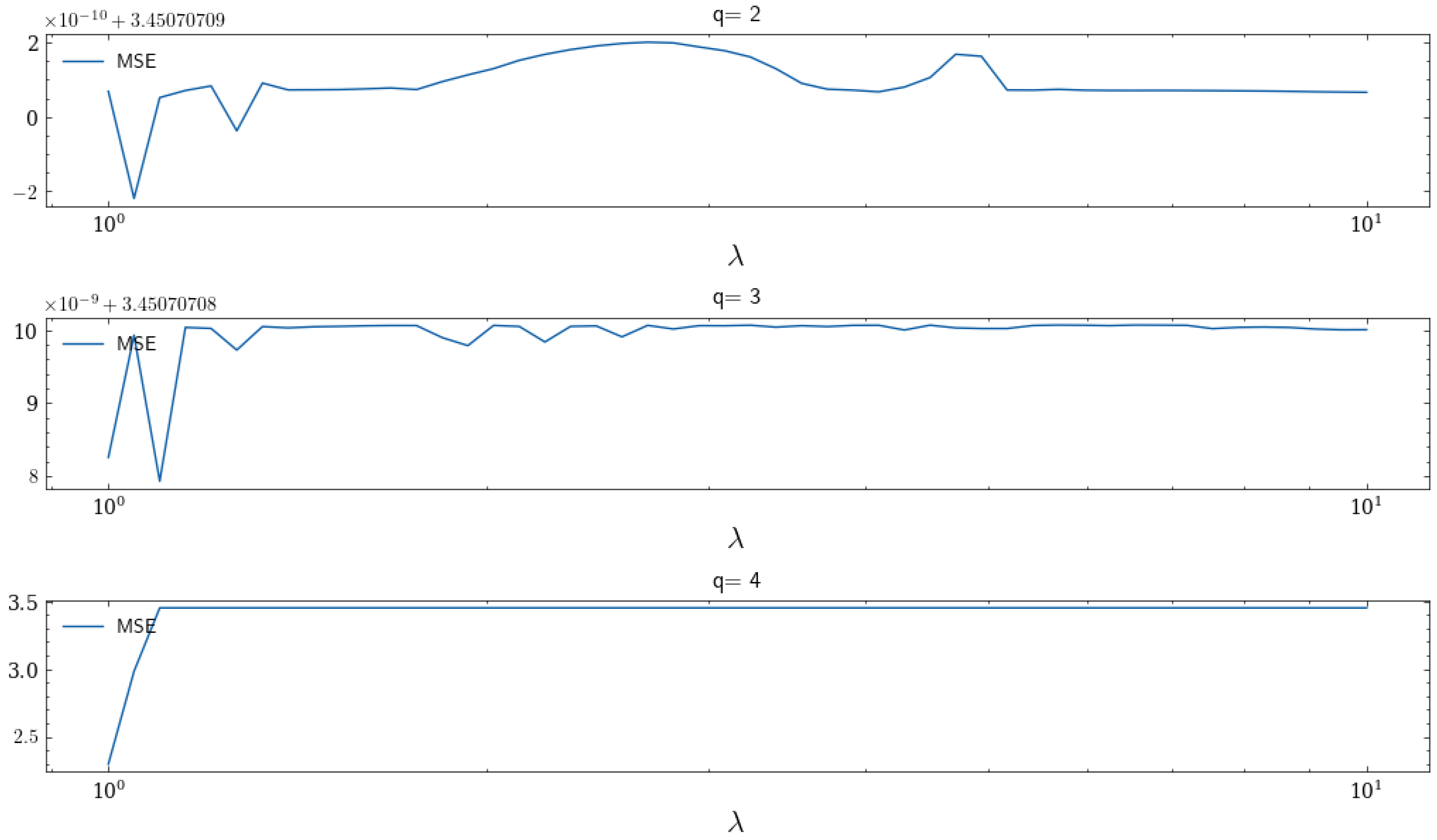
When $\alpha =\beta$, it reduces to the case of the classic Wasserstein metric. To illustrate their performance, we generate six hundred sets of samples with ${\mathbf{x}}_i^{\top }$ generated from the distribution $U(0,1)$ and $e_i$ generated from the distribution $N(0,1)$ independently and identically. The trend of MSE as $\lambda :=\frac{\alpha }{\beta }$ ranges from one to ten is presented below.

In Figure 1, we find that it is possible to achieve smaller MSE by adjusting the value of $\lambda$. Moreover, when $q=2$ and $q=3$, the value of $\lambda$ that minimizes MSE is larger than 1, which means that the shortfall–Wasserstein robust regression can achieve a better prediction effect than the Wasserstein robust regression.

Figure 1. MSE with respect to $\lambda$ for different values of q.

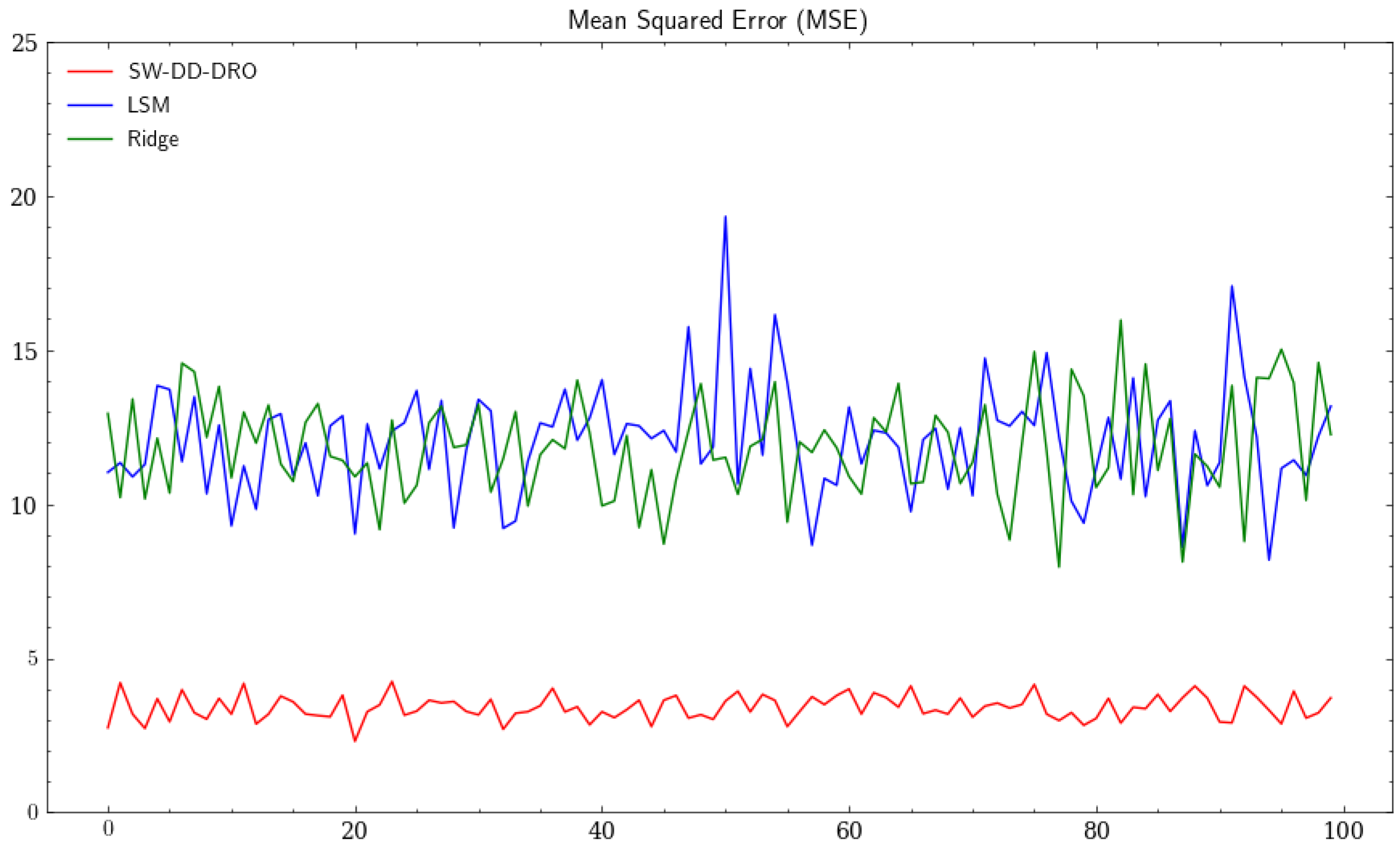
To test the robustness of our model, we further introduce some outliers and compare the performance with the least-squares regression (LSR) model and the ridge regression model. We set $\alpha =\beta$ for the shortfall–Wasserstein robust regression model and the regularization coefficient 1 for the ridge regression. We conduct one hundred times iterations, producing one hundred sets of samples each time, half of which served as the training set while the rest served as the testing set. Moreover, ten sets of outlier samples are added to the training set at each iteration. The result is presented below.

In Figure 2, the MSE under the shortfall–Wasserstein robust regression model is much smaller and less volatile than the MSE under the other two models, which means the shortfall–Wasserstein robust regression model is better in resisting the large deviations in the predictors. As a result, the result based on the shortfall–Wasserstein metric is reliable, stable, and superior to the one based on the Wasserstein metric.

Figure 2. The red, blue, and green curves represent the MSE under the SW-DD-DRO, the least-squares methods, and the ridge regression, respectively.

5.2. Portfolio Optimization

With $\mathit{\xi }$ being a random vector of returns from n different financial assets and $\mathit{\omega }$ being the allocation vector, the problem becomes a portfolio optimization problem. In this subsection, we take $l\left(X\right)={(X-c)}_{+}$ to characterize the downside risk, and the problem we are interested in is of the following form:

$$\underset{\mathit{\omega }\in \mathcal{D}}{inf}\underset{\mathbb{P}\in {\mathbb{B}}_{\epsilon }^{d_u}\left({\widehat{\mathbb{P}}}_N\right)}{sup}{\mathbb{E}}^{\mathbb{P}}{({\mathit{\omega }}^{\top }\mathit{\xi }-c)}_{+},$$

where c is a constant. By Corollary 2, with $u\left(x\right)=\alpha x_{+}-\beta x_{-},0<\alpha <\beta$, the inner maximum problem can be reformulated to the following form:

$$\frac{1}{N}\sum _{i=1}^N{({\mathit{\omega }}^{\top }{\widehat{\mathit{\xi }}}_i-c)}_{+}+\frac{\alpha }{\beta }{\parallel \mathit{\omega }\parallel }_q\epsilon .$$

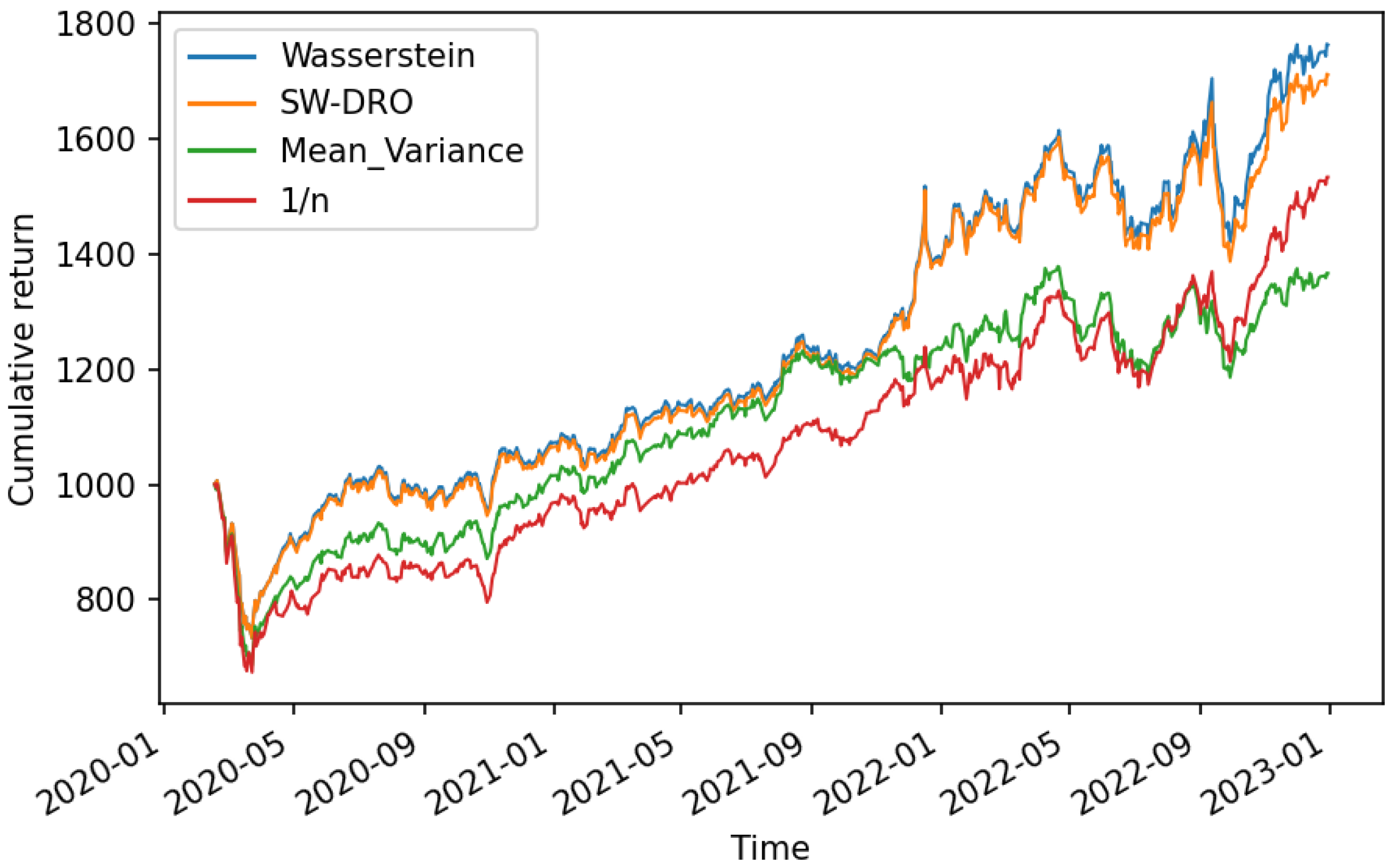
With the ambiguity set constructed by the classic Wasserstein metric, the result is the same as the form of the above formula with $\alpha =\beta$. For simulation, we choose four MSCI index assets, which are the MSCI Denmark index, the MSCI Turkey index, the MSCI Greece index, and the MSCI Norway index. We collect the daily closing prices of those indexes ranging from 1 January 2020 to 31 December 2022 from cn.investing.com. It is noteworthy that the COVID-19 outbreak began in 2020, and the distribution of assets is highly uncertain during this period. Based on those data, assume the initial asset is USD 1000 and there is no short sale. We set a 30-day time sliding window, the optimal weight is calculated based on the previous 30 days of historical data, and this result is taken as the investment decision of the next day. As the time window rolls, the cumulative return curves under different strategies are presented below.

The four curves represent the cumulative returns under the model constructed by the shortfall–Wasserstein metric with $\frac{\beta }{\alpha }=9$, the model constructed by the classic Wasserstein metric, the mean-variance model and the $\frac{1}{n}$ portfolio model, respectively. The mean-variance model, a model that aims to minimize investment variance under certain expected returns, was proposed by [24]. The $\frac{1}{n}$ portfolio model divides the money equally among each asset, and [25] found that the $\frac{1}{n}$ portfolio performs well when the overall distribution of assets is highly uncertain.

In Figure 3, we can see that the first two cumulative return curves under the robust optimization models outperform the curves under the mean-variance model and the $\frac{1}{n}$ portfolio model. Because of the similarity of the result of models under the shortfall–Wasserstein metric and the classic Wasserstein metric, the first two curves essentially behave the same. Since 2020, the global economy has been in recession due to the pandemic. In 2022, the epidemic was relatively stable and the economy slowly began to recover. During this period, the distribution of the four assets is highly uncertain. All four of these models perform well as the curves climb steadily, but the robust models take the variability into account and make better decisions, especially during the recovery period.

Figure 3. Cumulative return curves under different strategies.

In general, in regression problems, our results are more reliable and robust when the sample is contaminated; in portfolio optimization problems, when the distribution of assets is highly uncertain, our results perform significantly better. Moreover, our result can be more widely used than the result under the Wasserstein model as it is applicable for many complex forms of the function l. Even when the loss function $l(·)$ is relatively simple, our model can achieve the same or even better performance than the classic Wasserstein model by adjusting the form of the function $u(·)$.

6. Conclusions

In this paper, we propose a new DRO framework by extending the classic Wasserstein metrics to the shortfall–Wasserstein metrics. We study the tractability and reformulations of the shortfall–Wasserstein DRO problems for the loss function which is linear in the decision vector. This case of objective function includes many applications, such as regression and portfolio selection. One interesting result in the paper is that we give an equivalent characterization of the projection result to a one-dimensional ball. Based on the projection result, we show that the multi-dimensional constraint of our distributionally robust models can be reformulated as a one-dimensional one. Based on this reformulation, we established the finite sample guarantee of the DRO problem which is free from the curse of dimensionality. We present the application of our model in regression and provide simulation results to illustrate the performance of our results. In addition, we also present the real-data analysis on a portfolio selection to illustrate the performance of our new DRO model. Since this paper focuses on the linear cost function $l\left({\mathbf{w}}^{\top }\mathbf{x}\right)$, a possible future study is to consider the general loss function $l(\mathbf{w},\mathbf{x})$ and study the reformulations and tractability of the general DRO problems.

Appendix A.1. Strong Duality in Compact Spaces

To prepare for the verification, let us denote $C_S:=\{(x,y)\in S\times S,c(x,y)<+\infty \}$, ${\mathsf{\Lambda }}_{S,c,l}:=\{(\lambda ,\phi ):\lambda ⩾0,\phi \in {\mathcal{m}}_{\mathcal{U}}(S;\overline{\mathbb{R}}),\phi \left(x\right)+\lambda c(x,y)⩾l\left(y\right)forall(x,y)\in C_S\}$, and for $\forall \eta \in \mathbb{R}$, define

$$\overline{I_{\eta }}=sup\left\{\int l\left(y\right)d\pi (x,y):\pi \in \bigcup _{\nu \in \mathbb{P}\left(S\right)}\mathsf{\Pi }(\mu ,\nu ),\int cd\pi ⩽-\eta \right\},$$

$$\underline{J_{\eta }}=inf\{-\lambda \eta +\int \phi d\mu :(\lambda ,\phi )\in {\mathsf{\Lambda }}_{S,c,l}\}.$$

Proposition A1. 

Suppose S is a compact Polish space, and $l:S\to \mathbb{R}$ satisfies Assumption 4, $c(X,Y)=u\left(\right|Y-X|-{\epsilon }^{*})$, then for any $\eta \in \mathbb{R}$, $\overline{I_{\eta }}=\underline{J_{\eta }}$, and a primal optimizer ${\pi }_{\eta }^{*}$ satisfying $I\left({\pi }_{\eta }^{*}\right)=\overline{I_{\eta }}$ exists.

Proof. 

To prepare to apply the Fenchel duality theorem (see Theorem 1 in Chapter 7 of [26]), denote $X=C_b(S\times S)$ and its topological dual $X^{*}={\mathcal{M}}_b(S\times S)$, which is a consequence of the Riesz representation theorem. Next, let

$$C:=\{g(x,y)\in X:g(x,y)=\phi \left(x\right)+\lambda c(x,y)forallx,yforsome\phi \in C_b\left(S\right),\lambda ⩾0\},$$

$$D:=\left\{g\right(x,y)\in X:g(x,y)⩾l(y)foreveryx,y\}.$$

In the set C, each g is identified by the pair $(\lambda ,\phi )$

$$\phi \left(x\right)=g(x,x)-\lambda c(-{\epsilon }^{*}),\lambda =\frac{g(x,y)-g(x,x)+\lambda c(-{\epsilon }^{*})}{c(x,y)},$$

for some $x,y$ in S, $c(x,y)\ne 0$. Define functions $\mathsf{\Phi }:C\to \mathbb{R}$ and $\mathsf{\Gamma }:D\to \mathbb{R}$ as below:

$$\mathsf{\Phi }\left(g\right):=-\lambda \eta +\int \phi d\mu ,\mathsf{\Gamma }\left(g\right):=0.$$

From the definition, it is evident that the functional $\mathsf{\Phi }$ is convex and $\mathsf{\Gamma }$ is concave,

$$\underset{g\in C\cap D}{inf}\{\mathsf{\Phi }\left(g\right)-\mathsf{\Gamma }\left(g\right)\}=inf\left\{-\lambda \eta +\int \phi d\mu :\phi \left(x\right)+\lambda c(x,y)⩾l\left(y\right)forallx,yforsome\phi \in C_b\left(S\right),\lambda ⩾0\right\}.$$

The corresponding conjugate functions ${\mathsf{\Phi }}^{*}:C^{*}\to \mathbb{R}$ and ${\mathsf{\Gamma }}^{*}:D^{*}\to \mathbb{R}$ are as below:

$$C^{*}=\left\{\pi \in X^{*}:\underset{g\in C}{sup}[⟨g,\pi ⟩-\mathsf{\Phi }\left(g\right)]<+\infty \right\}=\left\{\pi \in X^{*}:\underset{g\in C}{sup}\left\{\int gd\pi -\mathsf{\Phi }\left(g\right)\right\}<+\infty \right\},$$

$$D^{*}=\left\{\pi \in X^{*}:\underset{g\in D}{inf}[⟨g,\pi ⟩-\mathsf{\Gamma }\left(g\right)]>-\infty \right\}=\left\{\pi \in X^{*}:\underset{g\in D}{inf}\int gd\pi >-\infty \right\},$$

$${\mathsf{\Phi }}^{*}\left(\pi \right)=\underset{g\in C}{sup}\left\{\int gd\pi -\mathsf{\Phi }\left(g\right)\right\},{\mathsf{\Gamma }}^{*}\left(\pi \right)=\underset{g\in D}{inf}\int gd\pi .$$

For every $\pi \in {\mathcal{M}}_b(S\times S)$,

$$\begin{array}{cc}\hfill \underset{g\in C}{sup}\left\{\int gd\pi -\mathsf{\Phi }\left(g\right)\right\}& =\underset{(\lambda ,\phi )\in R_{+}\times C_b\left(S\right)}{sup}\left\{\int \left(\phi \right(x)+\lambda c(x,y\left)\right)d\pi (x,y)-\int \phi \left(x\right)d\mu \left(x\right)+\lambda \eta \right\}\hfill \\ & =\underset{(\lambda ,\phi )\in R_{+}\times C_b\left(S\right)}{sup}\left\{\lambda \left(\int c(x,y)d\pi (x,y)+\eta \right)-\int \phi \left(x\right)(d\pi (x,y)-d\mu \left(x\right))\right\}\hfill \\ & =\left\{\begin{array}{c}0,if\int cd\pi ⩽-\eta and\pi (A\times S)=\mu \left(A\right)forallA\in \mathcal{B}\left(S\right),\hfill \\ \infty ,otherwise.\hfill \end{array}\right.\hfill \end{array}$$

Therefore,

$$C^{*}=\left\{\pi \in {\mathcal{M}}_b(S\times S):\int cd\pi ⩽-\eta ,\pi (A\times S)=\mu \left(A\right)forallA\in \mathcal{B}\left(S\right)\right\},{\mathsf{\Phi }}^{*}\left(\pi \right)=0.$$

Next, to determine $D^{*}$, we can see that if a measure $\pi \in {\mathcal{M}}_b(S\times S)$ is not non-negative, ${inf}_{g\in D}\int gd\pi =-\infty$ (for more details, see Lemma B.6 of [15]). When $\pi \in {\mathcal{M}}_b(S\times S)$ is non-negative, as l is an upper semicontinuous function that is bounded from above, we can use a monotonically decreasing sequence of continuous functions to approximate l point-by-point. As a result of the monotone convergence theorem, we have the following equality:

$$inf\left\{\int g(x,y)d\pi (x,y):g(x,y)⩾l\left(y\right)forallx,y\right\}=\int l\left(y\right)d\pi (x,y).$$

Then,

$$D^{*}=\left\{\pi \in {\mathcal{M}}_b(S\times S):\int l\left(y\right)d\pi (x,y)>-\infty \right\},{\mathsf{\Gamma }}^{*}\left(\pi \right)=\int l\left(y\right)\pi (x,y).$$

Then,

$${\mathsf{\Gamma }}^{*}\left(\pi \right)-{\mathsf{\Phi }}^{*}\left(\pi \right)=\int l\left(y\right)d\pi (x,y),$$

$$C^{*}\cap D^{*}=\left\{\pi \in \bigcup _{\nu \in \mathbb{P}\left(S\right)}\mathsf{\Pi }(\mu ,\nu ):\int cd\pi ⩽-\eta ,\int l\left(y\right)d\pi (x,y)>-\infty \right\}.$$

Then,

$$\overline{I_{\eta }}=sup\{{\mathsf{\Gamma }}^{*}\left(\pi \right)-{\mathsf{\Phi }}^{*}\left(\pi \right):\pi \in C^{*}\cap D^{*}\}.$$

Because there are some points of the relative interiors of C and D contained in the set $C\cap D$ and the epigraph of the function has a nonempty interior, further ${inf}_{g\in C\cap D}\{\mathsf{\Phi }\left(g\right)-\mathsf{\Gamma }\left(g\right)\}$ is finite, by the Fenchel’s duality theorem,

$$\underset{g\in C\cap D}{inf}\{\mathsf{\Phi }\left(g\right)-\mathsf{\Gamma }\left(g\right)\}=\underset{\pi \in C^{*}\cap D^{*}}{sup}\{{\mathsf{\Gamma }}^{*}\left(\pi \right)-{\mathsf{\Phi }}^{*}\left(\pi \right)\}=\overline{I_{\eta }}.$$

Moreover, some ${\pi }_{\eta }^{*}\in {\mathsf{\Phi }}_{\mu }$ that attain the supremum exist in the right. As $C_b\left(S\right)\subseteq {\mathcal{m}}_{\mathcal{U}}(S;\overline{\mathbb{R}})$, then

$$\underline{J_{\eta }}⩽inf\left\{-\lambda \eta +\int \phi d\mu :\phi \left(x\right)+\lambda c(x,y)⩾f\left(y\right)forallx,yforsome\phi \in C_b\left(S\right),\lambda ⩾0\right\}=\overline{I_{\eta }}.$$

Similar to the proof of weak duality, we can verify that $\overline{I_{\eta }}⩽\underline{J_{\eta }}$. Then we obtain $\overline{I_{\eta }}=\underline{J_{\eta }}$ and some ${\pi }_{\eta }^{*}$ exist such that $I\left({\pi }_{\eta }^{*}\right)=\overline{I_{\eta }}$. The proof is complete. □

Appendix A.2. Strong Duality in Non-Compact Spaces

Proposition A1 has established the strong duality in compact Polish spaces. We intend to extend the strong duality to $\mathbb{R}$, the verification is broken down into the following steps, and Proposition A2 is the first step.

For convenience, we first introduce some notations. For any $\pi \in \mathbb{P}(\mathbb{R}\times \mathbb{R})$, denote

$$S_{\pi }:=Spt\left({\pi }_X\right)\cup Spt\left({\pi }_Y\right),$$

in which $Spt\left({\pi }_X\right)$ and $Spt\left({\pi }_Y\right)$ are, respectively, referred to as the supports of marginals ${\pi }_X(·):=\pi (·\times \mathbb{R})$ and ${\pi }_Y(·):=\pi (\mathbb{R}\times ·)$. We have that the set $S_{\pi }\times S_{\pi }$ is $\sigma$-compact as every probability measure defined on a Polish space has $\sigma$-compact support; thus, in Proposition A2, $S_{\pi }\times S_{\pi }$ can be expressed as the union of an increasing sequence of compact subsets $(S_n\times S_n:n⩾1)$ [15]. Then we can apply the results of Proposition A1 via a sequential argument. For any closed subset $\mathbb{V}\subseteq \mathbb{R}$, let

$$\mathsf{\Lambda }(\mathbb{V}\times \mathbb{V}):=\{(\lambda ,\phi ):\lambda >0,\phi \in {\mathcal{m}}_{\mathcal{U}}(\mathbb{V};\overline{\mathbb{R}}),\phi \left(x\right)+\lambda c(x,y)⩾l\left(y\right)forall(x,y)\in (\mathbb{V}\times \mathbb{V})\cap C\},$$

where $C:=\left\{\right(x,y)\in \mathbb{R}\times \mathbb{R}:c(x,y)<\infty \}$ and ${\mathcal{m}}_{\mathcal{U}}(\mathbb{V};\overline{\mathbb{R}})$ denotes the set of measurable functions $\phi :(\mathbb{V},\mathcal{U}\left(\mathbb{V}\right))\to (\overline{\mathbb{R}},\mathcal{B}\left(\overline{\mathbb{R}}\right))$. With this notation, $\mathsf{\Lambda }(\mathbb{R}\times \mathbb{R})={\mathsf{\Lambda }}_{c,l}$. Furthermore, the function ${\phi }_{\lambda }\left(x\right):={sup}_{y\in S}\{l\left(y\right)-\lambda c(x,y)\}:(\mathbb{R},\mathcal{U}\left(\mathbb{R}\right)\to (\overline{\mathbb{R}},\mathcal{B}\left(\overline{\mathbb{R}}\right))$ is measurable. A more detailed explanation of this can be found in [15]. Finally, let us denote E as

$$E:=\left\{\pi \in \bigcup _{\nu \in \mathbb{P}\left(\mathbb{R}\right)}\mathsf{\Pi }(\mu ,\nu ):\int c(x,y)d\pi (x,y)<+\infty ,\int \left|l\left(y\right)\right|d\pi (x,y)<+\infty \right\}.$$

Proposition A2. 

If Assumption 4 holds and $c(X,Y)=u\left(\right|Y-X|-{\epsilon }^{*})$, then for any $\pi \in E$,

$$\underset{(\lambda ,\phi )\in \mathsf{\Lambda }(S_{\pi }\times S_{\pi })}{inf}J(\lambda ,\phi )⩽\overline{I}.$$

Proof. 

This proof is similar to [15]. We give a proof for completeness here. From the discussion above the proposition, we know that $S_{\pi }\times S_{\pi }$ is $\sigma$-compact. By the definition of $\sigma$-compactness, an increasing sequence of compact subsets of $S_n\times S_n$ exists such that $Spt\left(\pi \right)\subseteq S_{\pi }\times S_{\pi }={\cup }_{n⩾1}(S_n\times S_n)$. As $\int \left|l\right(y\left)\right|d\pi (x,y)$ and $\int c(x,y)d\pi (x,y)$ are finite, one is able to find $(S_n\times S_n,n⩾1)$ and $\eta \in (0,+\infty )$ to satisfy

$$p_n:=\pi (S_n\times S_n)⩾1-\frac{1}{n},$$

$$\int c(x,y)1_{{(S_n\times S_n)}^c}d\pi (x,y)⩽\frac{\eta }{n}(1-\frac{1}{n}),$$

$$\int \left|l\left(y\right)\right|1_{{(S_n\times S_n)}^c}d\pi (x,y)⩽\frac{1}{n},$$

where ${(S_n\times S_n)}^c:=(\mathbb{R}\times \mathbb{R})\setminus (S_n\times S_n)$. Define ${\pi }_n\in \mathbb{P}(S_n\times S_n)$ and its corresponding marginals ${\mu }_n\in \mathbb{P}\left(S_n\right)$ as below:

$${\pi }_n(·):=\frac{\pi (·\cap (S_n\times S_n))}{p_n},{\mu }_n(·):={\pi }_n(·\times S_n).$$

For every $n⩾1$, define

$$\overline{I_{\eta ,n}}:=sup\left\{\int l\left(y\right)\gamma (dx,dy):\gamma \in \underset{\nu \in \mathbb{P}\left(S_n\right)}{\cup }\mathsf{\Pi }({\mu }_n,\nu ),\int c(x,y)d\gamma (x,y)⩽-\frac{\eta }{n}\right\},$$

$$\underline{J_{\eta ,n}}:=inf\left\{-\lambda \frac{\eta }{n}+\int \phi d{\mu }_n:(\lambda ,\phi )\in \mathsf{\Lambda }(S_n\times S_n)\right\},$$

whose supports are $S_n\times S_n$. As $S_n$ is compact, from Proposition A1, we know that a ${\gamma }_{\eta ,n}^{*}\in \mathbb{P}(S_n\times S_n)$ exists, satisfying

$$\int l\left(y\right){\gamma }_{\eta ,n}^{*}(dx,dy)=\overline{I_{\eta ,n}}=\underline{J_{\eta ,n}}.$$

Construct a measure $\tilde{\pi }\in \mathbb{P}(\mathbb{R}\times \mathbb{R})$,

$$\tilde{\pi }(·)=p_n{\gamma }_{\eta ,n}^{*}(·\cap (S_n\times S_n))+\pi (·\cap {(S_n\times S_n)}^c).$$

It can be verified that $\tilde{\pi }\in \mathsf{\Pi }(\mu ,\nu )$ for some $\nu \in \mathbb{P}\left(\mathbb{R}\right)$. From the definition of $\tilde{\pi }$, we have

$$\begin{array}{cc}\hfill \tilde{\pi }(·\times \mathbb{R})& =p_n{\gamma }_{\eta ,n}^{*}((·\cap S_n)\times S_n)+\pi ((·\times \mathbb{R})\cap {(S_n\times S_n)}^c)\hfill \\ & =p_n{\mu }_n(·\cap S_n)+\pi ((·\times \mathbb{R})\cap {(S_n\times S_n)}^c)\hfill \\ & =\pi ((·\times \mathbb{R})\cap (S_n\times S_n))+\pi ((·\times \mathbb{R})\cap {(S_n\times S_n)}^c)\hfill \\ & =\pi (·\times \mathbb{R})=\mu (·),\hfill \end{array}$$

while the third equality is because ${\mu }_n(·)=\pi (·\times S_n)/p_n$, and $p_n{\mu }_n(·\cap S_n)=\pi ((·\cap \mathbb{R})\cap (S_n\times S_n))$. Furthermore,

$$\int cd\tilde{\pi }=p_n{\int }_{S_n\times S_n}cd{\gamma }_{\eta ,n}^{*}+{\int }_{{(S_n\times S_n)}^c}cd\pi ⩽-\frac{\eta }{n}(1-\frac{1}{n})+\frac{\eta }{n}(1-\frac{1}{n})=0.$$

Then, $\tilde{\pi }\in {\mathsf{\Phi }}_{\mu }$, and consequently,

$$\overline{I}⩾\int l\left(y\right)\tilde{\pi }(dx,dy)=p_n{\int }_{S_n\times S_n}ld{\gamma }_{\eta ,n}^{*}+{\int }_{{(S_n\times S_n)}^c}ld\pi .$$

Thus, we have $\overline{I}⩾p_n\overline{I_{\eta ,n}}-n^{-1}$, and as $\overline{I_{\eta ,n}}=\underline{J_{\eta ,n}}$, we have $\underline{J_{\eta ,n}}⩽{(1-\frac{1}{n})}^{-1}(\overline{I}+\frac{1}{n})$. Proposition A2 already holds when $\overline{I}=+\infty$, so we take $\overline{I}<+\infty$; for every $n⩾1$ and any $\epsilon >0$, take an $\epsilon$-optimal solution $({\lambda }_n,{\phi }_n)$ for $\underline{J_{\eta ,n}}$,

$$-{\lambda }_n\frac{\eta }{n}+\int {\phi }_{n}d{\mu }_n⩽\underline{J_{\eta ,n}}+\epsilon .$$

As $({\lambda }_n,{\phi }_n)$ belongs to $\mathsf{\Lambda }(S_n\times S_n)$, from definition, ${\phi }_n⩾{sup}_{z\in S_n}\{l\left(z\right)-{\lambda }_{n}c(x,z)\}$. Then, for every $x\in S_n$ and every n, we have

$$-{\lambda }_n\frac{\eta }{n}+\int \underset{z\in S_n}{sup}\{l\left(z\right)-{\lambda }_{n}c(x,z)\}d{\mu }_n\left(x\right)⩽\underline{J_{\eta ,n}}+\epsilon .$$

Combining the fact that ${\mu }_n(·)=\pi (·\times S_n)/p_n$, we further have

$$\overline{\underset{n\to \infty }{lim}}\left(-{\lambda }_n\frac{\eta }{n}+\int \underset{z\in S_n}{sup}\{l\left(z\right)-{\lambda }_{n}c(x,z)\}\frac{1_{s_n}\left(x\right)·1_{s_n}\left(y\right)}{p_n}d\pi (x,y)\right)⩽\overline{I}+\epsilon .$$

(A1)

Since $c(x,x)=c(-{\epsilon }^{*})>-\infty$, then $l\left(x\right)-{\lambda }_{n}c(-{\epsilon }^{*})$ is a lower bound of the integrand above on $S_n\times S_n$, and we also have $l\in L^1\left(d\mu \right)$, we obtain the following two results:

(a) From (A1) and the fact that ${\lambda }_n⩾0$, we have ${\stackrel{̲}{lim}}_{n\to \infty }{\lambda }_n,{\underline{lim}}_{n\to \infty }{\lambda }_n$ are finite, so $\{{\lambda }_n:n⩾1\}$ has convergent subsequences, which means that a subsequence $\{n_k:k⩾1\}$ exists at least such that ${\lambda }_{n_k}\to {\lambda }^{*}$ as $k\to \infty$ for some ${\lambda }^{*}\in [0,\infty )$;

(b) By Fatou’s lemma and dominated convergence theorem, we obtain

$$\begin{array}{cc}\hfill \overline{I}+\epsilon & ⩾\underset{k\to \infty }{\underline{lim}}\left(-{\lambda }_{n_k}\frac{\eta }{n_k}+\int \underset{z\in S_{n_k}}{sup}\{l\left(z\right)-{\lambda }_{n_k}c(x,z)\}\frac{1_{s_{n_k}}\left(x\right)·1_{s_{n_k}}\left(y\right)}{p_{n_k}}d\pi (x,y)\right)\hfill \\ & ⩾{\int }_{S_{\pi }\times S_{\pi }}\underset{z\in S_{\pi }}{sup}\{l\left(z\right)-{\lambda }^{*}c(x,z)\}d\pi (x,y)\hfill \\ & ={\int }_{S_{\pi }}\underset{z\in S_{\pi }}{sup}\{l\left(z\right)-{\lambda }^{*}c(x,z)\}d\mu \left(x\right).\hfill \end{array}$$

Here, these facts are used: $\frac{\eta }{n}\to 0,{\lambda }_n\to {\lambda }^{*}$ as $n\to \infty$ and $p_n\to 1,{\cup }_{n⩾1}{S}_n={\cup }_{k⩾1}{S}_{n_k}=S_{\pi }$. We also used the fact that ${\underline{lim}}_k{sup}_{z\in S_{n_k}}\{l\left(z\right)-{\lambda }_{n_k}c(x,z)\}⩾{sup}_{z\in S_{n_k}}\{l\left(z\right)-{\lambda }^{*}c(x,z)\}$ (see Lemma B.7 in Appendix B of [15]). If we let ${\phi }^{*}\left(x\right)={sup}_{z\in S_{\pi }}\{l\left(z\right)-{\lambda }^{*}c(x,z)\}$, then $({\lambda }^{*},{\phi }^{*})\in \mathsf{\Lambda }(S_{\pi }\times S_{\pi })$, and due to the arbitrariness of $\epsilon$, it follows that

$$J({\lambda }^{*},{\phi }^{*})⩽\overline{I}.$$

This completes the proof. □

Proposition A3. 

Suppose that Assumption 4 is in force, $c(X,Y)=u\left(\right|Y-X|-{\epsilon }^{*})$, then for any $\lambda ⩾0$,

$$\underset{\pi \in E}{sup}\int \{l\left(y\right)-\lambda c(x,y)\}d\pi (x,y)=\int \underset{z\in \mathbb{R}}{sup}\{l\left(z\right)-\lambda c(x,z)\}d\mu \left(x\right).$$

Proof. 

Let $g(x,y):=l\left(y\right)-\lambda c(x,y)$, for $n⩾1$ and $k⩽n^2$, define

$$A_{k,n}:=\left\{(x,y)\in \mathbb{R}\times \mathbb{R}:\frac{k-1}{n}⩽g(x,y)⩽\frac{k}{n}\right\},$$

$$B_{k,n}:=Pro{j}_1\left(A_{k,n}\right)\setminus {\cup }_{j>k}Pro{j}_1\left(A_{j,n}\right).$$

Noting that g is upper semicontinuous and the sets $A_{k,n}$ are Borel-measurable, we have that their projections $B_{k,n}$ are also Borel-measurable subsets of $\mathbb{R}$. Additionally, from the definition, the collection $(B_{k,n}:k⩽n^2)$ is disjoint. Then, due to the Jankov–von Neumann selection theorem [27], a universally measurable function ${\gamma }_k\left(x\right):Pro{j}_1\left(A_{k,n}\right)\to \mathbb{R}$ for each $k⩽n^2$ exits such that $A_{k,n}\ne \varnothing$, satisfying

$$\frac{k-1}{n}⩽g(x,{\gamma }_k\left(x\right))⩽\frac{k}{n}.$$

Next, as $B_{k,n}\subseteq Pro{j}_1\left(A_{k,n}\right)$ and $(B_{k,n}:k⩽n^2)$ is disjoint, we define ${\mathsf{\Gamma }}_n:\mathbb{R}\to \mathbb{R}$:

$${\mathsf{\Gamma }}_n\left(x\right):=\left\{\begin{array}{cc}{\gamma }_k\left(x\right),\hfill & \mathrm{if}x\in B_{k,n}\mathrm{for}\mathrm{some}k⩽n^2,\hfill \\ x,\hfill & \mathrm{otherwise}.\hfill \end{array}\right.$$

Since each ${\gamma }_k\left(x\right)$ is measurable, we have that ${\mathsf{\Gamma }}_n\left(x\right)$ is also measurable. For $\forall x\in \mathbb{R}$, if k exists such that $x\in B_{k,n}$, then $g(x,{\mathsf{\Gamma }}_k\left(x\right))=g(x,{\gamma }_k\left(x\right))⩾\frac{k-1}{n}$, and $sup\{g(x,y):g(x,y)⩽n,y\in S\}-\frac{1}{n}⩽\frac{k}{n}-\frac{1}{n}=\frac{k-1}{n}$. If such k do not exists, then $g(x,{\mathsf{\Gamma }}_k\left(x\right))=g(x,x)$ and $\left\{\right(x,y):g(x,y)⩽n,y\in S\}$ is an empty set, then we obtain

$$\begin{array}{c}\hfill sup\{g(x,y):g(x,y)⩽n,y\in \mathbb{R}\}-\frac{1}{n}⩽g(x,{\mathsf{\Gamma }}_n\left(x\right))⩽n.\end{array}$$

(A2)

Let $n\to \infty$, the we have

$$sup\{g(x,y):y\in \mathbb{R}\}⩽\underset{n\to \infty }{\underline{lim}}g(x,{\mathsf{\Gamma }}_n\left(x\right))⩽\infty .$$

Define the family of probability measures $({\pi }_n:n⩾1)$ as

$$d{\pi }_n(x,y)=d\mu \left(x\right)·d{\delta }_{{\mathsf{\Gamma }}_n\left(x\right)}\left(y\right).$$

From (A2), $g(x,y)⩽n,{\pi }_n$ almost surely; thus, $\int \left|c(x,y)\right|d{\pi }_n<+\infty$ and $\int \left|l\left(y\right)\right|d{\pi }_n<+\infty$. Moreover, since ${\pi }_n(·\times \mathbb{R})=\mu (·)$, then ${\pi }_n\in E$. Finally, since $g(x,{\mathsf{\Gamma }}_n\left(x\right))⩾l\left(x\right)-\lambda c(-{\epsilon }^{*})-1>-\infty$, by Fatou’s lemma,

$$\begin{array}{cc}\hfill \underset{n\to +\infty }{\underline{lim}}\int g(x,y)d{\pi }_n(x,y)& =\underset{n\to +\infty }{\underline{lim}}\int g(x,{\mathsf{\Gamma }}_n\left(x\right))d\mu \left(x\right)\hfill \\ & ⩾\int \underset{n\to +\infty }{\underline{lim}}g(x,{\mathsf{\Gamma }}_n\left(x\right))d\mu \left(x\right)\hfill \\ & ⩾\int \underset{y\in \mathbb{R}}{sup}g(x,y)d\mu \left(x\right).\hfill \end{array}$$

Then, ${sup}_{\pi \in E}\int gd\pi ⩾\int {sup}_{y\in \mathbb{R}}g(x,y)d\mu \left(x\right)$ holds. Since $\int gd\pi ⩽\int {sup}_{y\in \mathbb{R}}g(x,y)d\pi (x,y)$ for any $\pi \in E$, the proof is complete. □

Proof of Theorem 2. 

If $\overline{I}=\infty$, then $\overline{I}⩽\underline{J}=\infty$, the proof is complete. Consider the case that $\overline{I}<\infty$. As a result of Proposition A2, for every $\pi \in E$, we have

$$\overline{I}⩾\underset{(\lambda ,\phi )\in \mathsf{\Lambda }(S_{\pi }\times S_{\pi })}{inf}\left\{\int \phi \left(x\right)d\mu \left(x\right)\right\}⩾\underset{\lambda ⩾0}{inf}\left\{\int \underset{y\in S_{\pi }}{sup}\{l\left(y\right)-\lambda c(x,y)\}d\mu \left(x\right)\right\}.$$

(A3)

For any $\pi \in E$ and $\lambda ⩾0$, define

$$T(\lambda ,\pi ):=\int \underset{y\in S_{\pi }}{sup}\{l\left(y\right)-\lambda c(x,y)\}d\mu \left(x\right).$$

As $c(x.x)=c(-{\epsilon }^{*})$,

$$T(\lambda ,\pi )⩾\int ld\mu -\lambda c(-{\epsilon }^{*}).$$

(A4)

Since $T(\lambda ,\pi )>\overline{I}$ for every $\lambda >{\lambda }_{max}:=(\int ld\mu -\overline{I})/c(-{\epsilon }^{*})$, we restrict attention to the compact subset $[0,{\lambda }_{max}]$, from (A3), we can see

$$\overline{I}⩾\underset{\lambda \in [0,{\lambda }_{max}]}{inf}T(\lambda ,\pi ).$$

(A5)

As ${sup}_{y\in S_{\pi }}\{l\left(y\right)-\lambda c(x,y)\}$ is a lower semicontinuous function with respect to the variable $\lambda$, we can verify that $T(\lambda ,\pi )$ is lower semicontinuous in $\lambda$ as well. For any ${\lambda }_n\to \lambda$, as (A4) holds, we can apply Fatou’s lemma,

$$\begin{array}{cc}\hfill \underset{n\to +\infty }{\underline{lim}}T({\lambda }_n,\pi )& ⩾\int \underset{n}{\underline{lim}}\underset{y\in S_n}{sup}\{l\left(y\right)-{\lambda }_{n}c(x,y)\}d\mu \left(x\right)\hfill \\ & ⩾\int \underset{y\in S_n}{sup}\left\{l\right(y)-\lambda c(x,y\left)\right\}d\mu \left(x\right)=T(\lambda ,\pi ),\hfill \end{array}$$

$T(\lambda ,\pi )$ is a convex function with respect to $\lambda$ for fixed $\pi$. Additionally, for any $\alpha \in (0,1)$ and ${\pi }_1,{\pi }_2\in E$,

$$\begin{array}{cc}\hfill T(\lambda ,\alpha {\pi }_1+(1-\alpha ){\pi }_2)& =\int \underset{y\in S_{\alpha {\pi }_1+(1-\alpha ){\pi }_2}}{sup}\{l\left(y\right)-\lambda c(x,y)\}d\mu \left(x\right)\hfill \\ & ⩾\underset{i=1,2}{max}\left\{\int \underset{y\in S_{{\pi }_i}}{sup}\{l\left(y\right)-\lambda c(x,y)\}d\mu \left(x\right)\right\}\hfill \\ & ⩾\alpha T(\lambda ,{\pi }_1)+(1-\alpha )T(\lambda ,{\pi }_2),\hfill \end{array}$$

which means that $T(\lambda ,\pi )$ is concave in $\pi$ for fixed $\lambda$. By applying the minimax theorem, we can conclude

$$\underset{\pi \in E}{sup}\underset{\lambda \in [0,{\lambda }_{max}]}{inf}T(\lambda ,\pi )=\underset{\lambda \in [0,{\lambda }_{max}]}{inf}\underset{\pi \in E}{sup}T(\lambda ,\pi ).$$

In conjunction with (A5), the following is yielded:

$$\overline{I}⩾\underset{\pi \in E}{sup}\underset{\lambda \in [0,{\lambda }_{max}]}{inf}T(\lambda ,\pi )⩾\underset{\lambda \in [0,{\lambda }_{max}]}{inf}\left\{\underset{\pi \in E}{sup}\int \underset{y\in S_{\pi }}{sup}\{l\left(y\right)-\lambda c(x,y)\}d\mu \left(x\right)\right\}.$$

(A6)

Now, since $\int {sup}_{y\in S_{\pi }}\{l\left(y\right)-\lambda c(x,y)\}d\mu \left(x\right)⩾\int (l\left(y\right)-\lambda c(x,y))d\pi (x,y)$ for any $\pi \in E$, from Proposition A3, we have

$$\underset{\pi \in E}{sup}\int \underset{y\in S_{\pi }}{sup}\{l\left(y\right)-\lambda c(x,y)\}d\mu \left(x\right)=\int \underset{y\in \mathbb{R}}{sup}\{l\left(y\right)-\lambda c(x,y)\}d\mu \left(x\right)=\int {\phi }_{\lambda }\left(x\right)d\mu \left(x\right).$$

In conjunction with (A6), we further obtain

$$\overline{I}⩾\underset{\lambda \in [0,{\lambda }_{max}]}{inf}\int {\phi }_{\lambda }\left(x\right)d\mu \left(x\right)⩾\underset{\lambda ⩾0}{inf}\int {\phi }_{\lambda }\left(x\right)d\mu \left(x\right).$$

(A7)

Let $g\left(\lambda \right):=\int {\phi }_{\lambda }\left(x\right)d\mu \left(x\right)$, by Fatou’s lemma, ${\underline{lim}}_{n\to +\infty }g\left({\lambda }_n\right)⩾g\left(\lambda \right)$ as ${\lambda }_n\to \lambda ,$ then $g(·)$ is lower semicontinuous, and $g\left(\lambda \right)\to \infty$ when $\lambda \to \infty$ as $g\left(\lambda \right)⩾\int l\left(x\right)d\mu \left(x\right)-\lambda c(-{\epsilon }^{*})$ and $c(-{\epsilon }^{*})>0$. As a result, $\{\lambda :\lambda ⩾0,g(\lambda )⩽m\}$ are compact for every m. Therefore, $g(·)$ attains its infimum, i.e., we can find ${\lambda }^{*}\in [0,\infty )$ such that ${inf}_{\lambda ⩾0}\{\int {\phi }_{\lambda }\left(x\right)d\mu \left(x\right)\}=\int {\phi }_{{\lambda }^{*}}\left(x\right)d\mu \left(x\right)$. As ${\phi }_{{\lambda }^{*}}\left(x\right)+{\lambda }^{*}c(x,y)⩾l\left(y\right)$, we have $({\lambda }^{*},{\phi }_{{\lambda }^{*}})\in {\mathsf{\Lambda }}_{c,f}$; thus, $\underline{J}⩽\int {\phi }_{{\lambda }^{*}}\left(x\right)d\mu \left(x\right)$. In conjunction with (A7), we have $\overline{I}⩾\underline{J}$, then the proof of assertion(i) is complete.

Through the above verification, it is known that an optimizer of the dual problem $({\lambda }^{*},{\phi }_{{\lambda }^{*}})$ always exists. Next, if ${\pi }^{*}$ exists satisfying $\overline{I}=I\left({\pi }^{*}\right)=J({\lambda }^{*},{\phi }_{{\lambda }^{*}})$, which means it is an optimizer to the primal problem, then we have

$$\int l\left(y\right)d{\pi }^{*}(x,y)=\int {\phi }_{{\lambda }^{*}}\left(x\right)d\mu \left(x\right).$$

In addition, as ${\pi }^{*}\in {\mathsf{\Phi }}_{\mu }$ and ${\phi }_{{\lambda }^{*}}(x,y)={sup}_{y\in \mathbb{R}}\{l\left(y\right)-{\lambda }^{*}c(x,y)\}$:

$$\begin{array}{cc}\hfill \int l\left(y\right)d{\pi }^{*}(x,y)& =\int (l\left(y\right)-{\lambda }^{*}c(x,y))d{\pi }^{*}(x,y)+{\lambda }^{*}\int c(x,y)d{\pi }^{*}(x,y)\hfill \\ & ⩽\int {\phi }_{{\lambda }^{*}}(x,y)d{\pi }^{*}(x,y)+{\lambda }^{*}\int c(x,y)d{\pi }^{*}(x,y)\hfill \\ & ⩽\int {\phi }_{{\lambda }^{*}}(x,y)d{\pi }^{*}(x,y)=\int l\left(y\right)d{\pi }^{*}(x,y).\hfill \end{array}$$

Thus, we can conclude

$$l\left(y\right)-{\lambda }^{*}c(x,y)=\underset{z\in \mathbb{R}}{sup}\{l\left(z\right)-{\lambda }^{*}c(x,z)\}{\pi }^{*}a.s.,$$

(A8)

$${\lambda }^{*}\int c(x,y)d{\pi }^{*}(x,y)=0.$$

(A9)

Alternatively, if (A8) and (A9) are satisfied by any ${\pi }^{*}\in {\mathsf{\Phi }}_{\mu },({\lambda }^{*},{\phi }_{{\lambda }^{*}})\in \mathsf{\Lambda }(c,f)$,

$$\begin{array}{cc}\hfill \int l\left(y\right)d{\pi }^{*}(x,y)& =\int (l\left(y\right)-{\lambda }^{*}c(x,y))d{\pi }^{*}(x,y)+{\lambda }^{*}\int c(x,y)d{\pi }^{*}(x,y)\hfill \\ & =\int \underset{z\in \mathbb{R}}{sup}\{l\left(z\right)-{\lambda }^{*}c(x,z)\}d{\pi }^{*}(x,y)=\int {\phi }_{{\lambda }^{*}}\left(x\right)d\mu \left(x\right),\hfill \end{array}$$

which means that ${\pi }^{*}$ and $({\lambda }^{*},{\phi }_{{\lambda }^{*}})$ are optimal to the primal and dual problem. The proof of the uniqueness of the primal optimizer ${\pi }^{*}$ is similar to the proof of Theorem 1(b) in [15] and is, thus, omitted here. We then complete the proof. □