A Systematic Approach to Delay Functions

Abstract

We present a systematic introduction to a class of functions that provide fundamental solutions for autonomous linear integer-order and fractional-order delay differential equations. These functions, referred to as delay functions, are defined through power series or fractional power series, with delays incorporated into their series representations. Using this approach, we have defined delay exponential functions, delay trigonometric functions and delay fractional Mittag-Leffler functions, among others. We obtained Laplace transforms of the delay functions and demonstrated how they can be employed in finding solutions to delay differential equations. Our results, which extend and unify previous work, offer a consistent framework for defining and using delay functions.

1. Introduction

Special functions play a vital role in simplifying the analysis of many problems in mathematical physics and applied mathematics [1], especially in the solution of differential equations. For example, the exponential function and the Mittag-Leffler function [2,3] are fundamental in composing solutions for linear integer-order and linear fractional-order differential equations, respectively. Given the importance and prevalence of delay differential equations in mathematical modeling across a diverse array of disciplines, including biology [4,5], economics [4], engineering [6], pharmacokinetics [7], physics [8], population dynamics [9], and traffic modeling [4], it is natural to seek similar special functions for linear integer-order and linear fractional-order delay differential equations.

Indeed, there has been some progress in this direction, such as the Lambert W function [10] and delayed exponential functions for linear first-order delay differential equations [11,12], delay sine and cosine functions for linear second-order delay differential equations [13], and delayed Mittag-Leffler functions for fractional-order delay differential equations [14,15,16,17]. The introduction of such functions has proliferated in recent years; to date, this has been conducted in a non-uniform way, with varying notations and different types of series representations.

Certain special delay functions have been previously introduced for particular delay equations. In this work, we provide a systematic approach for obtaining representations to delay functions that provide solutions to delay differential equations. This provides a uniform representation of delay functions and it enables the identification of a large class of new delay functions that generalize special functions. First, we show how we can use the known series expansion solution of a given differential equation to create a corresponding delay function series expansion solution for a corresponding delay differential equation. In this way, we introduce a large class of previously unknown delay functions that provide solutions to delay differential equations. We then introduce a new solution method for delay differential equations by showing how solutions for arbitrary autonomous linear delay differential equations can be constructed from trial delay function series expansions. We also present the first table of Laplace transforms for delay functions, facilitating the use of Laplace transform methods in solving linear delay differential equations. Finally, we have generalized our approach using fractional power series and generalized power series to derive solutions for linear fractional-order delay differential equations and certain non-autonomous delay differential equations. This generalization is a further novel aspect of our systematic approach to delay functions as solutions of associated delay differential equations.

We hope that our approach will highlight the importance of delay functions, including those defined previously, and make them more accessible to a broader mathematics community. In general terms, delay functions are represented as truncated power series, truncated fractional power series, or truncated generalized power series, each incorporating a delay parameter $\sigma$, with the variable in the nth term of the series delayed by $n\sigma$. If the delay function is taken to be a function of a real variable, the series expansion can be truncated using a Heaviside function, which also facilitates the calculation of Laplace transform properties.

In Section 2, we define delay functions through truncated power series with delays incorporated in the series representation. Explicit definitions are given for delay exponential functions, delay trigonometric functions, delay hyperbolic trig functions, and delay hypergeometric functions. We calculated the derivatives of these functions and explored some of their basic properties. In Section 3, we define fractional delay functions through truncated fractional power series with delays incorporated in the series representation. Delay Mittag-Leffler functions and generalized delay Mittag-Leffler functions have been defined through this approach. In Section 4, we provide Laplace transform results for delay functions and fractional delay functions. In Section 5, we show how standard delay functions arise as solutions of autonomous linear integer-order delay differential equations, and in Section 6, we show how fractional delay functions arise as solutions of autonomous linear fractional-order delay differential equations. In Section 7, we introduce generalized power series delay functions and illustrate their application to a non-autonomous delay differential equation with a periodic coefficient. We provide a brief summary in Section 8.

2. Standard Delay Functions

Here, we define standard delay functions as truncated power series with the nth term delayed by $n\sigma$. The Heaviside function, which facilitates the analysis of truncated power series, is introduced first.

Definition 1.

The Heaviside function of a real variable x is defined as

$$\Theta \left(x\right)=\left\{\begin{array}{cc}0\hfill & x<0,\hfill \\ 1\hfill & x\ge 0.\hfill \end{array}\right.$$

(1)

See, for example, Lighthill [18], for further details on Heaviside and related functions.

Definition 2.

A delay function of a variable x with delay parameter σ is defined as

$$\mathrm{df}(x;\sigma )=\sum _{n=0}^{+\infty }{a}_n{(x-n\sigma )}^n\Theta \left(\frac{x}{\sigma }-n\right),\frac{x}{\sigma }\in \mathbb{R}.$$

(2)

The Heaviside function truncates the series expansion; thus, we can write

$$\mathrm{df}(x;\sigma )=\sum _{n=0}^{\lfloor \frac{x}{\sigma }\rfloor }{a}_n{(x-n\sigma )}^n,\frac{x}{\sigma }\in \mathbb{R}.$$

(3)

This explicit truncated form is preferred for defining delay functions over complex variables, $x,\sigma \in \mathbb{C}$, with $\frac{x}{\sigma }\in \mathbb{R}$. Note that if $\sigma \in {\mathbb{R}}_{>0}$, then the domain for the delay function is restricted to $x\in {\mathbb{R}}_{\ge 0}$, and conversely, if $\sigma \in {\mathbb{R}}_{<0}$, then the domain for the delay function is restricted to $x\in {\mathbb{R}}_{\le 0}$.

The definition of the delay function allows for a natural correspondence between a function and a delay function. This correspondence is noteworthy because some properties and relations of the original function have analogs in the delay function. In particular, this will allow us to correlate the solutions of certain ordinary differential equations with those of delay differential equations. In brief, for a real-valued function, $f\left(x\right)$, defined by a power series

$$f\left(x\right)=\sum _{n=0}^{+\infty }{a}_n{x}^n,x\in \mathbb{R},$$

(4)

we can define a corresponding delay function

$$\mathrm{df}(x;\sigma )=\sum _{n=0}^{+\infty }{a}_n{(x-n\sigma )}^n\Theta \left(\frac{x}{\sigma }-n\right),\frac{x}{\sigma }\in \mathbb{R},$$

(5)

which is convergent on the domain of $f\left(x\right)$. The convergence is assured by the truncation of the series in the definition of the delay function. The introduction of delay functions through infinite series expansions without the Heaviside function would typically lead to non-convergence. For example, if $f\left(x\right)$ is an analytic function with $a_n=\frac{f^{\left(n\right)}\left(0\right)}{n!}$, then ${\sum }_{n=0}^{+\infty }{a}_n{(x-n\sigma )}^n$ would fail the nth term test at $x=0,\sigma =1$; viz ${\lim }_{n\to +\infty }\frac{n^n}{n!}\to +\infty$.

Example 1.

If we consider the exponential function,

$$\exp \left(x\right)=\sum _{n=0}^{+\infty }\frac{x^n}{\Gamma (n+1)},$$

(6)

then we can define a corresponding delay function

$$\mathrm{df}(x;\sigma )=\sum _{n=0}^{+\infty }\frac{{(x-n\sigma )}^n}{\Gamma (n+1)}\Theta \left(\frac{x}{\sigma }-n\right),\frac{x}{\sigma }\in \mathbb{R}.$$

(7)

If we consider the exponential function,

$$\exp (-x)=\sum _{n=0}^{+\infty }{(-1)}^n\frac{x^n}{\Gamma (n+1)},$$

(8)

then we can define a corresponding delay function

$$\mathrm{dg}(x;\sigma )=\sum _{n=0}^{+\infty }{(-1)}^n\frac{{(x-n\sigma )}^n}{\Gamma (n+1)}\Theta \left(\frac{x}{\sigma }-n\right),\frac{x}{\sigma }\in \mathbb{R}.$$

(9)

Note that with these definitions, $\mathrm{df}(-x;-\sigma )=\mathrm{dg}(x;\sigma )$.

To avoid possible ambiguity, we define the delay exponential function below.

Definition 3.

The delay exponential function is defined as

$$\mathrm{dexp}(x;\sigma )=\sum _{n=0}^{+\infty }\frac{{(x-n\sigma )}^n}{\Gamma (n+1)}\Theta \left(\frac{x}{\sigma }-n\right),\frac{x}{\sigma }\in \mathbb{R}.$$

(10)

A delayed exponential function, similar to the above, has been previously introduced using a slightly different notation in [11,12]. It immediately follows from Definition 3 that

$$\mathrm{dexp}(\lambda x;\lambda \sigma )=\sum _{n=0}^{+\infty }\frac{{\lambda }^n{(x-n\sigma )}^n}{\Gamma (n+1)}\Theta \left(\frac{x}{\sigma }-n\right),\frac{x}{\sigma }\in \mathbb{R},\lambda \in \mathbb{C},$$

(11)

which identifies the parameter $\lambda$ as a common scale factor for x and $\sigma$.

Alternative representations of this function are also possible. For example, if $t>0$ and $0<\tau <\frac{1}{e}$, then we can use Laplace transform methods, as shown below, to write

$$\mathrm{dexp}(-t;-\tau )=\sum _{k\in \mathbb{Z}}^{+\infty }\frac{\exp \left(\frac{W_k(-\tau )}{\tau }t\right)}{1+W_k(-\tau )},$$

(12)

where $W_k\left(z\right)$ denotes the kth branch of the Lambert W function [10], which satisfies

$$W_k\left(z\right)\exp \left(W_k\left(z\right)\right)=z$$

(13)

with

$$\underset{\left|z\right|\to +\infty }{\lim }{W}_k\left(z\right)\to {\ln }_{k}z=\ln z+2\pi ik.$$

(14)

Figure 1 shows plots of the delay exponential functions $\mathrm{dexp}(x;\sigma )$ and $\mathrm{dexp}(-x;-\sigma )$ for three different delay values. For positive x and $\sigma$, the behavior is similar to the standard exponential function, with the growth slower for larger delays. For negative x and $\sigma$, the behavior is similar to the standard exponential function for very small delays, but for larger delays, the delay exponential function exhibits oscillatory behavior.

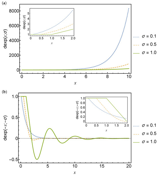
Figure 1. Plots of the delay exponential functions $\mathrm{dexp}(x;\sigma )$ (a) and $\mathrm{dexp}(-x;-\sigma )$ (b) for delays $\sigma =0.1,0.5,1.0$. The solid green line is for $\sigma =1.0$ and the dashed blue and red lines are for $\sigma =0.1$ and $\sigma =0.5$, respectively.

The following lemma shows that the derivative of the delay exponential function is proportional to the function itself but with x replaced by $x-\sigma$.

Lemma 1.

The derivative of the delay exponential function is given by

$$\frac{d}{dx}\mathrm{dexp}(\lambda x;\lambda \sigma )=\lambda \mathrm{dexp}(\lambda (x-\sigma );\lambda \sigma ),\frac{x}{\sigma }\in \mathbb{R}\setminus \left\{0\right\},\lambda \in \mathbb{C}.$$

(15)

Proof. 

We first note that the nth-generalized derivative of the Heaviside function is given by

$${\Theta }^{\left(n\right)}\left(x\right)={\delta }^{(n-1)}\left(x\right),$$

(16)

where ${\delta }^{(n-1)}\left(x\right)$ denotes the ($n-1$)th derivative of the Dirac delta generalized function $\delta \left(x\right)$. Hence, by differentiating Equation (11), term-by-term, gives

$$\begin{array}{cc}\hfill \frac{d}{dx}\mathrm{dexp}(\lambda x;\lambda \sigma )& =\sum _{n=1}^{+\infty }\frac{{\lambda }^n{(x-n\sigma )}^{n-1}}{\Gamma \left(n\right)}\Theta \left(\frac{x}{\sigma }-n\right)\hfill \\ \hfill & +\sum _{n=0}^{+\infty }\frac{{\lambda }^n{(x-n\sigma )}^n}{\Gamma (n+1)}\frac{1}{\sigma }\delta \left(\frac{x}{\sigma }-n\right)\hfill \end{array}$$

(17)

$$\begin{array}{cc}\hfill & =\lambda \sum _{n=0}^{+\infty }\frac{{\lambda }^n{((x-\sigma )-n\sigma )}^n}{\Gamma (n+1)}\Theta \left(\frac{x-\sigma }{\sigma }-n\right)\hfill \end{array}$$

(18)

$$\begin{array}{cc}\hfill & =\lambda \mathrm{dexp}\left(\lambda \right(x-\sigma );\lambda \sigma ),\hfill \end{array}$$

(19)

where the only contribution from the Dirac delta sum is when $n=0$ but this term vanishes on the domain $\frac{x}{\sigma }\in \mathbb{R}\setminus \left\{0\right\}$. □

We next focus on delay trigonometric functions and begin with the definition of the delay cosine and delay sine functions.

Definition 4.

The delay cosine function is defined as

$$\mathrm{dcos}(x;\sigma )=\sum _{n=0}^{+\infty }{(-1)}^n\frac{{(x-\left(2n\right)\sigma )}^{2n}}{\Gamma (2n+1)}\Theta \left(\frac{x}{\sigma }-2n\right),\frac{x}{\sigma }\in \mathbb{R}.$$

(20)

Definition 5.

The delay sine function is defined as

$$\mathrm{dsin}(x;\sigma )=\sum _{n=0}^{+\infty }{(-1)}^n\frac{{(x-(2n+1)\sigma )}^{2n+1}}{\Gamma (2n+2)}\Theta \left(\frac{x}{\sigma }-2n-1\right),\frac{x}{\sigma }\in \mathbb{R}.$$

(21)

The delay sine and cosine functions were previously introduced by [13] in connection with second-order delay differential equations.

It is evident from Definitions 4 and 5 that $\mathrm{dcos}(-x;-\sigma )=\mathrm{dcos}(x;\sigma )$ and $\mathrm{dsin}(-x;-\sigma )=-\mathrm{dsin}(x;\sigma )$, which mirrors the even and odd nature of the cosine and sine functions, respectively. Plots of the delay cosine and delay sine functions are shown in Figure 2 for three different delay values. These delay functions are oscillatory but not periodic for finite delays. Also, the amplitude of the oscillations increases as the delay increases.

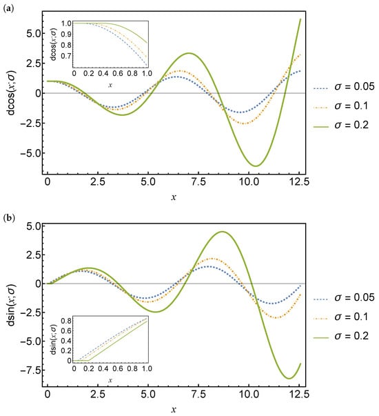
Figure 2. Plots of the delay cosine function $\mathrm{dcos}(x;\sigma )$ (a) and the delay sine function $\mathrm{dsin}(x;\sigma )$ (b) for delays $\sigma =0.05,0.1,0.2$. The solid green line is for $\sigma =0.2$ and the dashed blue and red lines are for $\sigma =0.05$ and $\sigma =0.1$, respectively.

The next lemma shows that the derivatives of the delay cosine and delay sine functions are analogous to the derivatives of their non-delay counterparts.

Lemma 2.

The derivatives of the delay cosine and delay sine functions are given by

$$\frac{d}{dx}\mathrm{dcos}(\lambda x;\lambda \sigma )=-\lambda \mathrm{dsin}(\lambda (x-\sigma );\lambda \sigma ),\frac{x}{\sigma }\in \mathbb{R}\setminus \left\{0\right\},\lambda \in \mathbb{C},$$

(22)

and

$$\frac{d}{dx}\mathrm{dsin}(\lambda x;\lambda \sigma )=\lambda \mathrm{dcos}(\lambda (x-\sigma );\lambda \sigma ),\frac{x}{\sigma }\in \mathbb{R},\lambda \in \mathbb{C},$$

(23)

respectively.

Proof. 

We verify Equation (22) by differentiating Equation (20) term-by-term, with x and $\sigma$ scaled by the parameter $\lambda$, to give

$$\begin{array}{cc}\hfill & \frac{d}{dx}\mathrm{dcos}(\lambda x;\lambda \sigma )\hfill \end{array}$$

$$\begin{array}{cc}\hfill & =\sum _{n=1}^{+\infty }{(-1)}^n\frac{{\lambda }^{2n}{(x-\left(2n\right)\sigma )}^{2n-1}}{\Gamma \left(2n\right)}\Theta \left(\frac{x}{\sigma }-2n\right)\hfill \\ \hfill & +\sum _{n=0}^{+\infty }{(-1)}^n\frac{{\lambda }^{2n}{(x-\left(2n\right)\sigma )}^{2n}}{\Gamma (2n+1)}\frac{1}{\sigma }\delta \left(\frac{x}{\sigma }-2n\right)\hfill \end{array}$$

(24)

$$\begin{array}{cc}\hfill & =-\lambda \sum _{n=0}^{+\infty }{(-1)}^n\frac{{\lambda }^{2n+1}{((x-\sigma )-(2n+1)\sigma )}^{2n+1}}{\Gamma (2n+2)}\Theta \left(\frac{x-\sigma }{\sigma }-2n-1\right)\hfill \end{array}$$

(25)

$$\begin{array}{cc}\hfill & =-\lambda \mathrm{dsin}\left(\lambda \right(x-\sigma );\lambda \sigma ),\hfill \end{array}$$

(26)

where we note that the only contribution from the Dirac delta sum is when $n=0$ but this term vanishes on the domain $\frac{x}{\sigma }\in \mathbb{R}\setminus \left\{0\right\}$. Similarly, Equation (23) follows by differentiating Equation (21) term-by-term, with x and $\sigma$ scaled by the parameter $\lambda$, to give

$$\begin{array}{cc}\hfill & \frac{d}{dx}\mathrm{dsin}(\lambda x;\lambda \sigma )\hfill \end{array}$$

$$\begin{array}{cc}\hfill & =\sum _{n=0}^{+\infty }{(-1)}^n\frac{{\lambda }^{2n+1}{(x-(2n+1)\sigma )}^{2n}}{\Gamma (2n+1)}\Theta \left(\frac{x}{\sigma }-2n-1\right)\hfill \\ \hfill & +\sum _{n=0}^{+\infty }{(-1)}^n\frac{{\lambda }^{2n+1}{(x-(2n+1)\sigma )}^{2n+1}}{\Gamma (2n+2)}\frac{1}{\sigma }\delta \left(\frac{x}{\sigma }-2n-1\right)\hfill \end{array}$$

(27)

$$\begin{array}{cc}\hfill & =\lambda \sum _{n=0}^{+\infty }{(-1)}^n\frac{{\lambda }^{2n}{((x-\sigma )-\left(2n\right)\sigma )}^{2n}}{\Gamma (2n+1)}\Theta \left(\frac{x-\sigma }{\sigma }-2n\right)\hfill \end{array}$$

(28)

$$\begin{array}{cc}\hfill & =\lambda \mathrm{dcos}\left(\lambda \right(x-\sigma );\lambda \sigma ),\hfill \end{array}$$

(29)

where we note that the Dirac delta sum vanishes for all $n\ge 0$. □

The following proposition shows that Euler’s formula $e^{ix}=\cos \left(x\right)+i\sin \left(x\right)$ can be extended to delay functions.

Proposition 1.

Euler’s formula for delay functions is given by the equation

$$\mathrm{dexp}(ix;i\sigma )=\mathrm{dcos}(x;\sigma )+i\mathrm{dsin}(x;\sigma ),\frac{x}{\sigma }\in \mathbb{R}.$$

(30)

Proof. 

Starting with Equation (11), where $\lambda =i$, we observe that

$$\begin{array}{cc}\hfill \mathrm{dexp}& (ix;i\sigma )\hfill \end{array}$$

$$\begin{array}{cc}\hfill & =\sum _{n=0}^{\lfloor \frac{x}{\sigma }\rfloor }\frac{i^n{(x-n\sigma )}^n}{\Gamma (n+1)}\hfill \end{array}$$

(31)

$$\begin{array}{cc}\hfill & =\sum _{k=0}^{\lfloor \frac{x}{2\sigma }\rfloor }\frac{i^{2k}{(x-2k\sigma )}^{2k}}{\Gamma (2k+1)}+\sum _{k=0}^{\lfloor \frac{x+\sigma }{2\sigma }\rfloor -1}\frac{i^{2k+1}{(x-(2k+1)\sigma )}^{2k+1}}{\Gamma (2k+2)}\hfill \end{array}$$

(32)

$$\begin{array}{cc}\hfill & =\sum _{k=0}^{\lfloor \frac{x}{2\sigma }\rfloor }{(-1)}^k\frac{{(x-2k\sigma )}^{2k}}{\Gamma (2k+1)}+i\sum _{k=0}^{\lfloor \frac{x+\sigma }{2\sigma }\rfloor -1}{(-1)}^k\frac{{(x-(2k+1)\sigma )}^{2k+1}}{\Gamma (2k+2)}\hfill \end{array}$$

(33)

$$\begin{array}{cc}\hfill & =\mathrm{dcos}(x;\sigma )+i\mathrm{dsin}(x;\sigma ).\hfill \end{array}$$

(34)

□

Using Proposition 1, we can obtain other identities involving delay trigonometric functions. An example of such an identity is given in the following corollary.

Corollary 1.

A relation between the delay cosine and delay sine functions is given by

$$\mathrm{dexp}(ix;i\sigma )\mathrm{dexp}(-ix;-i\sigma )={\mathrm{dcos}}^2(x;\sigma )+{\mathrm{dsin}}^2(x;\sigma ),\frac{x}{\sigma }\in \mathbb{R}.$$

(35)

Proof. 

From Proposition 1, we can write

$$\mathrm{dexp}(ix;i\sigma )\mathrm{dexp}(-ix;-i\sigma )=\left(\mathrm{dcos}(x;\sigma )-i\mathrm{dsin}(x;\sigma )\right)\left(\mathrm{dcos}(x;\sigma )+i\mathrm{dsin}(x;\sigma )\right),$$

(36)

which simplifies to yield Equation (35). □

We can also formulate the delay cosine and delay sine functions in terms of delay exponential functions in a similar manner as their non-delay counterparts.

Corollary 2.

The delay cosine and delay sine functions have a delay exponential representation given by

$$\mathrm{dcos}(x;\sigma )=\frac{1}{2}\left(\mathrm{dexp}(ix;i\sigma )+\mathrm{dexp}(-ix;-i\sigma )\right),\frac{x}{\sigma }\in \mathbb{R},$$

(37)

and

$$\mathrm{dsin}(x;\sigma )=\frac{1}{2i}\left(\mathrm{dexp}(ix;i\sigma )-\mathrm{dexp}(-ix;-i\sigma )\right),\frac{x}{\sigma }\in \mathbb{R},$$

(38)

respectively.

Proof. 

It follows from Proposition 1 that

$$\mathrm{dcos}(x;\sigma )=\mathrm{dexp}(ix;i\sigma )-i\mathrm{dsin}(x;\sigma )$$

(39)

and replacing i with $-i$ in Equation (30), we arrive at

$$i\mathrm{dsin}(x;\sigma )=\mathrm{dcos}(x;\sigma )-\mathrm{dexp}(-ix;-i\sigma ).$$

(40)

Substituting Equation (40) into Equation (39) and rearranging, we obtain Equation (37). Similarly, it follows from Proposition 1 that

$$i\mathrm{dsin}(x;\sigma )=\mathrm{dexp}(ix;i\sigma )-\mathrm{dcos}(x;\sigma )$$

(41)

and replacing i with $-i$ in Equation (30), we arrive at

$$\mathrm{dcos}(x;\sigma )=\mathrm{dexp}(-ix;-i\sigma )+i\mathrm{dsin}(x;\sigma ).$$

(42)

Substituting Equation (42) into Equation (41) and rearranging, we obtain Equation (38). □

The delay cosine and delay sine functions both have an analog delay hyperbolic function, which we define next.

Definition 6.

The delay hyperbolic cosine function is defined as

$$\mathrm{dcosh}(x;\sigma )=\sum _{n=0}^{+\infty }\frac{{(x-\left(2n\right)\sigma )}^{2n}}{\Gamma (2n+1)}\Theta \left(\frac{x}{\sigma }-2n\right),\frac{x}{\sigma }\in \mathbb{R}.$$

(43)

Definition 7.

The delay hyperbolic sine function is defined as

$$\mathrm{dsinh}(x;\sigma )=\sum _{n=0}^{+\infty }\frac{{(x-(2n+1)\sigma )}^{2n+1}}{\Gamma (2n+2)}\Theta \left(\frac{x}{\sigma }-2n-1\right),\frac{x}{\sigma }\in \mathbb{R}.$$

(44)

It is clear from the above definitions that $\mathrm{dcosh}(-x;-\sigma )=\mathrm{dcosh}(x;\sigma )$ and $\mathrm{dsinh}(-x;-\sigma )=-\mathrm{dsinh}(x;\sigma )$, mirroring the even and odd nature of the hyperbolic cosine and hyperbolic sine functions, respectively.

Plots of the delay hyperbolic cosine and delay hyperbolic sine functions are shown in Figure 3 for three different delay values.

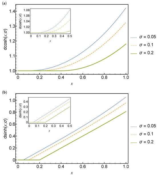
Figure 3. Plots of the delay hyperbolic cosine function $\mathrm{dcosh}(x;\sigma )$ (a) and the delay hyperbolic sine function $\mathrm{dsinh}(x;\sigma )$ (b) for delays $\sigma =0.05,0.1,0.2$. The solid green line is for $\sigma =0.2$ and the dashed blue and red lines are for $\sigma =0.05$ and $\sigma =0.1$, respectively.

The derivatives of the delay hyperbolic cosine and delay hyperbolic sine functions closely resemble the derivatives of their non-delay counterparts.

Lemma 3.

The derivative of the delay hyperbolic cosine and delay hyperbolic sine functions are given by

$$\frac{d}{dx}\mathrm{dcosh}(\lambda x;\lambda \sigma )=\lambda \mathrm{dsinh}(\lambda (x-\sigma );\lambda \sigma ),\frac{x}{\sigma }\in \mathbb{R}\setminus \left\{0\right\},\lambda \in \mathbb{C},$$

(45)

and

$$\frac{d}{dx}\mathrm{dsinh}(\lambda x;\lambda \sigma )=\lambda \mathrm{dcosh}(\lambda (x-\sigma );\lambda \sigma ),\frac{x}{\sigma }\in \mathbb{R},\lambda \in \mathbb{C},$$

(46)

respectively.

Proof. 

The method to verify Equations (45) and (46) is almost identical to that presented in Lemma 2 but with the initial removal of the ${(-1)}^n$ term from Equations (24) and (27). □

The next theorem shows that the hyperbolic identity $\exp \left(x\right)=\cosh \left(x\right)+\sinh \left(x\right)$ can be extended to delay functions.

Proposition 2.

The delay hyperbolic cosine and delay hyperbolic sine functions satisfy the equation

$$\mathrm{dexp}(x;\sigma )=\mathrm{dcosh}(x;\sigma )+\mathrm{dsinh}(x;\sigma ),\frac{x}{\sigma }\in \mathbb{R}.$$

(47)

Proof. 

Starting with Equation (10), we observe that

$$\begin{array}{cc}\hfill \mathrm{dexp}(x;\sigma )& =\sum _{n=0}^{\lfloor \frac{x}{\sigma }\rfloor }\frac{{(x-n\sigma )}^n}{\Gamma (n+1)}\hfill \end{array}$$

(48)

$$\begin{array}{cc}\hfill & =\sum _{k=0}^{\lfloor \frac{x}{2\sigma }\rfloor }\frac{{(x-2k\sigma )}^{2k}}{\Gamma (2k+1)}+\sum _{k=0}^{\lfloor \frac{x+\sigma }{2\sigma }\rfloor -1}\frac{{(x-(2k+1)\sigma )}^{2k+1}}{\Gamma (2k+2)}\hfill \end{array}$$

(49)

$$\begin{array}{cc}\hfill & =\sum _{k=0}^{\lfloor \frac{x}{2\sigma }\rfloor }\frac{{(x-2k\sigma )}^{2k}}{\Gamma (2k+1)}+\sum _{k=0}^{\lfloor \frac{x+\sigma }{2\sigma }\rfloor -1}\frac{{(x-(2k+1)\sigma )}^{2k+1}}{\Gamma (2k+2)}\hfill \end{array}$$

(50)

$$\begin{array}{cc}\hfill & =\mathrm{dcosh}(x;\sigma )+\mathrm{dsinh}(x;\sigma ).\hfill \end{array}$$

(51)

□

Using Proposition 2, we can obtain other identities involving delay hyperbolic trig functions. An example of such an identity is stated in the next corollary.

Corollary 3.

A relation between the delay hyperbolic cosine and delay hyperbolic sine functions is given by

$$\mathrm{dexp}(x;\sigma )\mathrm{dexp}(-x;-\sigma )={\mathrm{dcosh}}^2(x;\sigma )-{\mathrm{dsinh}}^2(x;\sigma ),\frac{x}{\sigma }\in \mathbb{R}.$$

(52)

Proof. 

From Proposition 2, we can write

$$\mathrm{dexp}(x;\sigma )\mathrm{dexp}(-x;-\sigma )=\left(\mathrm{dcosh}(x;\sigma )+\mathrm{dsinh}(x;\sigma )\right)\left(\mathrm{dcosh}(x;\sigma )-\mathrm{dsinh}(x;\sigma )\right),$$

(53)

which simplifies to yield Equation (52). □

We can also express the delay hyperbolic cosine and delay hyperbolic sine functions in terms of delay exponential functions.

Corollary 4.

The delay hyperbolic cosine and delay hyperbolic sine functions have a delay exponential representation given by

$$\mathrm{dcosh}(x;\sigma )=\frac{1}{2}\left(\mathrm{dexp}(x;\sigma )+\mathrm{dexp}(-x;-\sigma )\right),\frac{x}{\sigma }\in \mathbb{R},$$

(54)

and

$$\mathrm{dsinh}(x;\sigma )=\frac{1}{2}\left(\mathrm{dexp}(x;\sigma )-\mathrm{dexp}(-x;-\sigma )\right),\frac{x}{\sigma }\in \mathbb{R},$$

(55)

respectively.

Proof. 

It follows from Proposition 2 that

$$\mathrm{dcosh}(x;\sigma )=\mathrm{dexp}(x;\sigma )-\mathrm{dsinh}(x;\sigma )$$

(56)

and setting $x=-x$ and $\sigma =-\sigma$ in Equation (47), we arrive at

$$\mathrm{dsinh}(x;\sigma )=\mathrm{dcosh}(x;\sigma )-\mathrm{dexp}(-x;-\sigma ).$$

(57)

Substituting Equation (57) into Equation (56) and rearranging, we obtain Equation (54). Similarly, it follows from Proposition 2 that

$$\mathrm{dsinh}(x;\sigma )=\mathrm{dexp}(x;\sigma )-\mathrm{dcosh}(x;\sigma ),$$

(58)

and setting $x=-x$ and $\sigma =-\sigma$ in Equation (47), we arrive at

$$\mathrm{dcosh}(x;\sigma )=\mathrm{dexp}(-x;-\sigma )+\mathrm{dsinh}(x;\sigma ).$$

(59)

Substituting Equation (59) into Equation (58) and rearranging, we obtain Equation (55). □

We can use the known series expansions of the inverse hyperbolic trigonometric functions to construct corresponding series expansions for delay inverse hyperbolic trig functions. It is important to note that the delay inverse hyperbolic trig functions are not inverse functions for the delay hyperbolic trig functions. The delay inverse hyperbolic trig functions do however share some of the other properties with their non-delay counterparts. This is highlighted in the following example.

Example 2.

Starting with the series expansion for the inverse hyperbolic tangent function

$$\mathrm{arctanh}\left(x\right)=\sum _{n=0}^{+\infty }\frac{x^{2n+1}}{2n+1},\left|x\right|<1,$$

(60)

we identify the corresponding delay inverse hyperbolic tangent function

$$\mathrm{darctanh}(x;\sigma )=\sum _{n=0}^{+\infty }\frac{{(x-(2n+1)\sigma )}^{2n+1}}{2n+1}\Theta \left(\frac{x}{\sigma }-2n-1\right),\left|x\right|<1.$$

(61)

The derivative of the inverse hyperbolic tangent function is

$$\frac{d}{dx}\mathrm{arctanh}\left(x\right)=\sum _{n=0}^{+\infty }{x}^{2n},\left|x\right|<1,$$

(62)

which we recognize as the series expansion for

$$f\left(x\right)=\frac{1}{1-x^2},\left|x\right|<1.$$

(63)

The derivative of the delay inverse hyperbolic tangent function is

$$\begin{array}{cc}\hfill \frac{d}{dx}\mathrm{darctanh}(x;\sigma )& =\sum _{n=0}^{+\infty }{(x-(2n+1)\sigma )}^{2n}\Theta \left(\frac{x}{\sigma }-2n-1\right),\left|x\right|<1,\hfill \end{array}$$

(64)

$$\begin{array}{cc}\hfill & =\sum _{n=0}^{+\infty }{((x-\sigma )-2n\sigma )}^{2n}\Theta \left(\frac{x-\sigma }{\sigma }-2n\right),\left|x\right|<1,\hfill \end{array}$$

(65)

$$\begin{array}{cc}\hfill & =\mathrm{df}(x-\sigma ;\sigma ),\hfill \end{array}$$

(66)

where

$$\mathrm{df}(x;\sigma )=\sum _{n=0}^{+\infty }{(x-2n\sigma )}^{2n}\Theta \left(\frac{x}{\sigma }-2n\right),\left|x\right|<1,$$

(67)

is the corresponding delay function for $f\left(x\right)$ defined above. Thus, the derivative of the delay inverse hyperbolic tangent function is the corresponding delay function for the derivative of the standard inverse hyperbolic tangent function.

We now formulate the delay function of the hypergeometric function. We begin with a definition.

Definition 8.

The delay hypergeometric function is defined as

$${}_p{\mathrm{dF}}_q(a_1,\dots ,a_p;b_1,\dots ,b_q;x;\sigma )=\sum _{n=0}^{+\infty }\frac{{\prod }_{i=1}^p{\left(a_i\right)}^{\overline{n}}}{{\prod }_{j=1}^q{\left(b_j\right)}^{\overline{n}}}\frac{{(x-n\sigma )}^n}{\Gamma (n+1)}\Theta \left(\frac{x}{\sigma }-n\right),\frac{x}{\sigma }\in \mathbb{R}.$$

(68)

Here, ${\left(c\right)}^{\overline{n}}$ denotes the rising factorial Pochhammer symbol for $n\ge 0$, i.e. ${\left(c\right)}^{\overline{0}}=1$, ${\left(c\right)}^{\overline{1}}=c$ and ${\left(c\right)}^{\overline{n}}=c(c+1)\cdots (c+n-1)$ for $n>1$.

The next lemma presents the derivative of the delay hypergeometric function.

Lemma 4.

The derivative of the delay hypergeometric function is given by

$$\begin{array}{cc}\hfill & \frac{d}{dx}{}_p{\mathrm{dF}}_q(a_1,\dots ,a_p;b_1,\dots ,b_q;x;\sigma )\hfill \\ & =\frac{{\prod }_{i=1}^p{a}_i}{{\prod }_{j=1}^q{b}_j}{}_p{\mathrm{dF}}_q(a_1+1,\dots ,a_p+1;b_1+1,\dots ,b_q+1;x-\sigma ;\sigma ),\frac{x}{\sigma }\in \mathbb{R}\setminus \left\{0\right\}.\hfill \end{array}$$

(69)

Proof. 

Differentiating Equation (68) term-by-term gives

$$\begin{array}{cc}\hfill & \frac{d}{dx}{}_p{\mathrm{dF}}_q(a_1,\dots ,a_p;b_1,\dots ,b_q;x;\sigma )\hfill \end{array}$$

$$\begin{array}{cc}\hfill & =\sum _{n=1}^{+\infty }\frac{{\prod }_{i=1}^p{\left(a_i\right)}^{\overline{n}}}{{\prod }_{j=1}^q{\left(b_j\right)}^{\overline{n}}}\frac{{(x-n\sigma )}^{n-1}}{\Gamma \left(n\right)}\Theta \left(\frac{x}{\sigma }-n\right)\hfill \\ \hfill & +\sum _{n=0}^{+\infty }\frac{{\prod }_{i=1}^p{\left(a_i\right)}^{\overline{n}}}{{\prod }_{j=1}^q{\left(b_j\right)}^{\overline{n}}}\frac{{(x-n\sigma )}^n}{\Gamma (n+1)}\frac{1}{\sigma }\delta \left(\frac{x}{\sigma }-n\right)\hfill \end{array}$$

(70)

$$\begin{array}{cc}\hfill & =\sum _{n=0}^{+\infty }\frac{{\prod }_{i=1}^p{\left(a_i\right)}^{\overline{n+1}}}{{\prod }_{j=1}^q{\left(b_j\right)}^{\overline{n+1}}}\frac{{((x-\sigma )-n\sigma )}^n}{\Gamma (n+1)}\Theta \left(\frac{x-\sigma }{\sigma }-n\right)\hfill \end{array}$$

(71)

$$\begin{array}{cc}\hfill & =\frac{{\prod }_{i=1}^p{a}_i}{{\prod }_{j=1}^q{b}_j}\sum _{n=0}^{+\infty }\frac{{\prod }_{i=1}^p{(a_i+1)}^{\overline{n}}}{{\prod }_{j=1}^q{(b_j+1)}^{\overline{n}}}\frac{{((x-\sigma )-n\sigma )}^n}{\Gamma (n+1)}\Theta \left(\frac{x-\sigma }{\sigma }-n\right)\hfill \end{array}$$

(72)

$$\begin{array}{cc}\hfill & =\frac{{\prod }_{i=1}^p{a}_i}{{\prod }_{j=1}^q{b}_j}{}_p{\mathrm{dF}}_q(a_1+1,\dots ,a_p+1;b_1+1,\dots ,b_q+1;x-\sigma ;\sigma ),\hfill \end{array}$$

(73)

where we note that the only contribution from the Dirac delta sum is when $n=0$ but this term vanishes on the domain $\frac{x}{\sigma }\in \mathbb{R}\setminus \left\{0\right\}$. □

3. Fractional Delay Functions

Here, we define fractional delay functions based on fractional power series, which have been proven to be useful for solving fractional-order differential equations [19,20,21]. We begin with the definition of a fractional power series.

Definition 9.

The fractional power series of a real function, $f\left(t\right)$, is an infinite series of the form

$$f\left(t\right)=\sum _{n=0}^{+\infty }{a}_{\alpha ,n}{t}^{\alpha n},0<\alpha <1,t\ge 0.$$

(74)

We now expand our definition of delay functions by defining fractional delay functions, which may prove useful for solving fractional delay equations.

Definition 10.

For $0<\alpha <1$, a fractional delay function of a variable x with delay parameter σ is defined as

$${\mathrm{df}}_{\alpha }(x;\sigma )=\sum _{n=0}^{+\infty }{a}_{\alpha ,n}{(x-n\sigma )}^{\alpha n}\Theta \left(\frac{x}{\sigma }-n\right),\frac{x}{\sigma }\in \mathbb{R}.$$

(75)

Arguably, the most fundamental function in fractional calculus is the function $e_{\alpha }\left(x\right)=E_{\alpha }(-x^{\alpha })$ [3], where

$$E_{\alpha }\left(x\right)=\sum _{n=0}^{+\infty }\frac{x^n}{\Gamma (\alpha n+1)}$$

(76)

is the Mittag-Leffler function and the parameter $\alpha \in (0,1)$. The fractional power series representation of the function $e_{\alpha }\left(x\right)$ can be used as a basis to define delay fractional Mittag-Leffler functions.

Definition 11.

For $0<\alpha <1$, the delay fractional Mittag-Leffler function is defined as

$${\mathrm{dE}}_{\alpha }^{+}(x;\sigma )=\sum _{n=0}^{+\infty }\frac{{(x-n\sigma )}^{\alpha n}}{\Gamma (\alpha n+1)}\Theta \left(\frac{x}{\sigma }-n\right),\frac{x}{\sigma }\in \mathbb{R},$$

(77)

and

$${\mathrm{dE}}_{\alpha }^{-}(-x;-\sigma )=\sum _{n=0}^{+\infty }{(-1)}^n\frac{{(x-n\sigma )}^{\alpha n}}{\Gamma (\alpha n+1)}\Theta \left(\frac{x}{\sigma }-n\right),\frac{x}{\sigma }\in \mathbb{R}.$$

(78)

The delay Mittag-Leffler function, similar to Equation (77) for $x\in {\mathbb{R}}^{+}$, was introduced as a solution of a linear homogeneous [15] and a linear non-homogeneous [14,17] fractional-order delay differential equation. Note that our notation for the delay fractional Mittag-Leffler function follows the notation used for general fractional delay functions stated in Definition 10.

Plots of the delay fractional Mittag-Leffler function ${\mathrm{dE}}_{\alpha }^{-}(-x;-\sigma )$ with $\alpha =0.8,0.2$ are shown in Figure 4 for three different delay values. The delay fractional Mittag-Leffler function ${\mathrm{dE}}_{\alpha }^{-}(-x;-\sigma )$ has larger amplitude oscillations for larger delays. The oscillations are smoother for larger values of $\alpha$. Further study is needed to determine if the oscillations vanish for sufficiently small $\sigma$ and sufficiently large $\alpha ⪅1$.

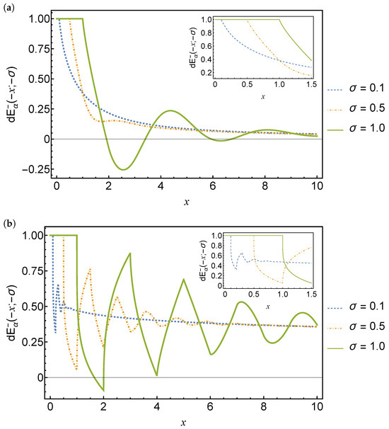
Figure 4. Plots of the delay fractional Mittag-Leffler function ${\mathrm{dE}}_{\alpha }^{-}(-x;-\sigma )$ with $\alpha =0.8$ (a) and $\alpha =0.2$ (b) for delays $\sigma =0.1,0.5,1.0$. The solid green line is for $\sigma =1.0$ and the dashed blue and red lines are for $\sigma =0.1$ and $\sigma =0.5$, respectively.

Next, we generalize the delay fractional Mittag-Leffler function given by Equation (77) via the inclusion of two additional parameters.

Definition 12.

For $0<\alpha <1$ and $\beta ,\gamma \in {\mathbb{R}}_{\ge 0}$, the generalized delay fractional Mittag-Leffler function is defined as

$${\mathrm{dE}}_{\alpha ,\beta ,\gamma }^{+}(x;\sigma )=\sum _{n=0}^{+\infty }\frac{{(x-n\sigma )}^{\alpha n+\gamma }}{\Gamma (\alpha n+\beta )}\Theta \left(\frac{x}{\sigma }-n\right),\frac{x}{\sigma }\in \mathbb{R}.$$

(79)

Interestingly, we can express the derivative of the generalized delay fractional Mittag-Leffler function, Equation (79), as a linear combination of three generalized delay fractional Mittag-Leffler functions, but with different parameters and arguments.

Lemma 5.

For $0<\alpha <1$ and $\beta ,\gamma \in {\mathbb{R}}_{\ge 0}$, the derivative of the generalized delay fractional Mittag-Leffler function is given by

$$\begin{array}{cc}\hfill \frac{d}{dx}{\mathrm{dE}}_{\alpha ,\beta ,\gamma }^{+}(x;\sigma )& =\gamma {\mathrm{dE}}_{\alpha ,\beta ,\gamma -1}^{+}(x;\sigma )\hfill \\ & +{\mathrm{dE}}_{\alpha ,\alpha +\beta -1,\alpha +\gamma -1}^{+}(x-\sigma ;\sigma )\hfill \\ & -(\beta -1){\mathrm{dE}}_{\alpha ,\alpha +\beta ,\alpha +\gamma -1}^{+}(x-\sigma ;\sigma ),\frac{x}{\sigma }\in \mathbb{R}\setminus \left\{0\right\}.\hfill \end{array}$$

(80)

Proof. 

Differentiating Equation (79) term-by-term gives

$$\begin{array}{cc}\hfill \frac{d}{dx}{\mathrm{dE}}_{\alpha ,\beta ,\gamma }^{+}(x;\sigma )& =\sum _{n=1}^{+\infty }\frac{\alpha n{(x-n\sigma )}^{\alpha n+\gamma -1}}{\Gamma (\alpha n+\beta )}\Theta \left(\frac{x}{\sigma }-n\right)\hfill \\ \hfill & +\gamma \sum _{n=0}^{+\infty }\frac{{(x-n\sigma )}^{\alpha n+\gamma -1}}{\Gamma (\alpha n+\beta )}\Theta \left(\frac{x}{\sigma }-n\right)\hfill \\ \hfill & +\sum _{n=0}^{+\infty }\frac{{(x-n\sigma )}^{\alpha n+\gamma }}{\Gamma (\alpha n+\beta )}\frac{1}{\sigma }\delta \left(\frac{x}{\sigma }-n\right)\hfill \end{array}$$

(81)

$$\begin{array}{cc}\hfill & =\sum _{n=1}^{+\infty }\frac{\alpha n{(x-n\sigma )}^{\alpha n+\gamma -1}}{\Gamma (\alpha n+\beta )}\Theta \left(\frac{x}{\sigma }-n\right)+\gamma {\mathrm{dE}}_{\alpha ,\beta ,\gamma -1}^{+}(x;\sigma ),\hfill \end{array}$$

(82)

where we note that the Dirac delta sum vanishes on the domain $\frac{x}{\sigma }\in \mathbb{R}\setminus \left\{0\right\}$, irrespective of the value of $\gamma \in {\mathbb{R}}_{\ge 0}$. We then simplify the remaining sum in Equation (82) by replacing

$$\frac{\alpha n}{\Gamma (\alpha n+\beta )}=\frac{1}{\Gamma (\alpha n+\beta -1)}-\frac{(\beta -1)}{\Gamma (\alpha n+\beta )},$$

(83)

so that

$$\begin{array}{cc}\hfill & \sum _{n=1}^{+\infty }\frac{\alpha n{(x-n\sigma )}^{\alpha n+\gamma -1}}{\Gamma (\alpha n+\beta )}\Theta \left(\frac{x}{\sigma }-n\right)\hfill \end{array}$$

$$\begin{array}{cc}\hfill & =\sum _{n=1}^{+\infty }\frac{{(x-n\sigma )}^{\alpha n+\gamma -1}}{\Gamma (\alpha n+\beta -1)}\Theta \left(\frac{x}{\sigma }-n\right)\hfill \\ \hfill & -(\beta -1)\sum _{n=1}^{+\infty }\frac{{(x-n\sigma )}^{\alpha n+\gamma -1}}{\Gamma (\alpha n+\beta )}\Theta \left(\frac{x}{\sigma }-n\right)\hfill \end{array}$$

(84)

$$\begin{array}{cc}\hfill & =\sum _{n=0}^{+\infty }\frac{{((x-\sigma )-n\sigma )}^{\alpha n+\alpha +\gamma -1}}{\Gamma (\alpha n+\alpha +\beta -1)}\Theta \left(\frac{x-\sigma }{\sigma }-n\right)\hfill \\ \hfill & -(\beta -1)\sum _{n=0}^{+\infty }\frac{{((x-\sigma )-n\sigma )}^{\alpha n+\alpha +\gamma -1}}{\Gamma (\alpha n+\alpha +\beta )}\Theta \left(\frac{x-\sigma }{\sigma }-n\right)\hfill \end{array}$$

(85)

$$\begin{array}{cc}\hfill & ={\mathrm{dE}}_{\alpha ,\alpha +\beta -1,\alpha +\gamma -1}^{+}(x-\sigma ;\sigma )\hfill \\ \hfill & -(\beta -1){\mathrm{dE}}_{\alpha ,\alpha +\beta ,\alpha +\gamma -1}^{+}(x-\sigma ;\sigma ).\hfill \end{array}$$

(86)

Substituting the results from Equation (86) into Equation (82), we obtain Equation (80). □

The following lemma provides two special cases of Lemma 5.

Lemma 6.

For $0<\alpha <1$, two derivatives of the generalized delay fractional Mittag-Leffler function with different values for β and γ are given by

$$\frac{d}{dx}{\mathrm{dE}}_{\alpha ,1,0}^{+}(x;\sigma )={\mathrm{dE}}_{\alpha ,\alpha ,\alpha -1}^{+}(x-\sigma ;\sigma ),\frac{x}{\sigma }\in \mathbb{R}\setminus \left\{0\right\},$$

(87)

and

$$\frac{d}{dx}{\mathrm{dE}}_{\alpha ,1,1}^{+}(x;\sigma )={\mathrm{dE}}_{\alpha ,1,0}^{+}(x;\sigma )+{\mathrm{dE}}_{\alpha ,\alpha ,\alpha }^{+}(x-\sigma ;\sigma ),\frac{x}{\sigma }\in \mathbb{R}\setminus \left\{0\right\}.$$

(88)

Proof. 

This follows from an application of Lemma 5 with the specified values of $\beta$ and $\gamma$. □

4. Laplace Transform Results

In this section, we derive results that enable the Laplace transform of both standard and fractional delay functions to be readily determined. These results essentially rely on finding the delay function corresponding to the given power series and then taking the Laplace transform term-by-term of the resulting sum.

4.1. Standard Delay Functions

We first consider the Laplace transform of standard delay functions.

Theorem 1.

If $f\left(t\right)$ permits a power series representation, Equation (4), with Laplace transform

$${\mathcal{L}}_t\left[f\left(t\right)\right]\left(s\right)={\int }_0^{+\infty }{e}^{-st}f\left(t\right)dt=\widehat{f}\left(s\right),s\in \mathbb{C},$$

(89)

then the Laplace transform of the corresponding delay function $\mathrm{df}(t;\tau )$ is given by

$${\mathcal{L}}_t\left[\mathrm{df}(t;\tau )\right]\left(s\right)=e^{s\tau }\widehat{f}\left(s{e}^{s\tau }\right),\tau >0,$$

(90)

and

$${\mathcal{L}}_t\left[\mathrm{df}(\lambda t;\lambda \tau )\right]\left(s\right)=\frac{1}{\lambda }{e}^{s\tau }\widehat{f}\left(\frac{s}{\lambda }{e}^{s\tau }\right),\lambda \in \mathbb{C},\tau >0.$$

(91)

Proof. 

Starting with the power series

$$f\left(t\right)=\sum _{n=0}^{+\infty }{a}_n{t}^n$$

(92)

we take the Laplace transform term-by-term with

$${\mathcal{L}}_t\left[t^n\right]\left(s\right)=\Gamma (1+n)s^{-(1+n)}$$

(93)

to obtain

$$\widehat{f}\left(s\right)=\sum _{n=0}^{+\infty }{a}_n\Gamma (1+n)s^{-(1+n)}.$$

(94)

From Equation (92), we identify the corresponding standard delay function

$$\mathrm{df}(t;\tau )=\sum _{n=0}^{+\infty }{a}_n{(t-n\tau )}^n\Theta \left(\frac{t}{\tau }-n\right),$$

(95)

and we take the Laplace transform term-by-term and use

$${\mathcal{L}}_t\left[{(t-n\tau )}^n\Theta \left(\frac{t}{\tau }-n\right)\right]\left(s\right)=\Gamma (1+n)s^{-(1+n)}{e}^{-sn\tau }$$

(96)

to write

$$\begin{array}{cc}\hfill {\mathcal{L}}_t\left[\mathrm{df}(t;\tau )\right]\left(s\right)& =\sum _{n=0}^{+\infty }{a}_n\Gamma (1+n)s^{-(1+n)}{e}^{-sn\tau }\hfill \end{array}$$

(97)

$$\begin{array}{cc}\hfill & =e^{s\tau }\sum _{n=0}^{+\infty }{a}_n\Gamma (1+n){\left(s{e}^{s\tau }\right)}^{-(1+n)}\hfill \end{array}$$

(98)

$$\begin{array}{cc}\hfill & =e^{s\tau }\widehat{f}\left(s{e}^{s\tau }\right)\hfill \end{array}$$

(99)

$$\begin{array}{cc}\hfill & =\widehat{\mathrm{d}}\mathrm{f}(s;\tau ).\hfill \end{array}$$

(100)

The second result follows in a similar manner. Starting with

$$\mathrm{df}(\lambda t;\lambda \tau )=\sum _{n=0}^{+\infty }{a}_n{\lambda }^n{(t-n\tau )}^n\Theta \left(\frac{t}{\tau }-n\right)$$

(101)

and proceeding as above, we have

$$\begin{array}{cc}\hfill {\mathcal{L}}_t\left[\mathrm{df}(\lambda t;\lambda \tau )\right]\left(s\right)& =\sum _{n=0}^{+\infty }{a}_n{\lambda }^n\Gamma (1+n)s^{-(1+n)}{e}^{-sn\tau }\hfill \end{array}$$

(102)

$$\begin{array}{cc}\hfill & =\frac{1}{\lambda }{e}^{s\tau }\sum _{n=0}^{+\infty }{a}_n\Gamma (1+n){\left(\frac{s}{\lambda }{e}^{s\tau }\right)}^{-(1+n)}\hfill \end{array}$$

(103)

$$\begin{array}{cc}\hfill & =\frac{1}{\lambda }{e}^{\frac{s}{\lambda }\lambda \tau }\sum _{n=0}^{+\infty }{a}_n\Gamma (1+n){\left(\frac{s}{\lambda }{e}^{\frac{s}{\lambda }\lambda \tau }\right)}^{-(1+n)}\hfill \end{array}$$

(104)

$$\begin{array}{cc}\hfill & =\frac{1}{\lambda }\widehat{\mathrm{d}}\mathrm{f}\left(\frac{s}{\lambda };\lambda \tau \right).\hfill \end{array}$$

(105)

□

The following example demonstrates how the previous theorem can be used to obtain the Laplace transform of a standard delay function.

Example 3.

The exponential function, defined by the power series,

$$\exp \left(t\right)=\sum _{n=0}^{+\infty }\frac{t^n}{\Gamma (n+1)}$$

(106)

has Laplace transform

$${\mathcal{L}}_t\left[\exp \left(t\right)\right]\left(s\right)=\frac{1}{s-1}.$$

(107)

It then follows from Theorem 1 that the corresponding delay exponential function has Laplace transform

$${\mathcal{L}}_t\left[\mathrm{dexp}(t;\tau )\right]\left(s\right)=e^{s\tau }\frac{1}{s{e}^{s\tau }-1}=\frac{1}{s-e^{-s\tau }}.$$

(108)

Thus, in this example, we have

$$\widehat{\mathrm{d}}\mathrm{f}(s;\tau )=\frac{1}{s-e^{-s\tau }}.$$

(109)

It then follows from Equation (105) with $\lambda =-1$ that

$${\mathcal{L}}_t\left[\mathrm{dexp}(-t;-\tau )\right]\left(s\right)=-\widehat{\mathrm{d}}\mathrm{f}(-s;-\tau )=\frac{1}{s+e^{-s\tau }}.$$

(110)

Example 4.

The representation of the delay exponential function $\mathrm{dexp}(-t;-\tau )$ in terms of Lambert W functions, Equation (12), can now be recovered by finding the inverse Laplace transform of

$${\mathcal{L}}_t\left[\mathrm{dexp}(-t;-\tau )\right]\left(s\right)=\frac{1}{s+e^{-s\tau }}=F\left(s\right),$$

(111)

using the complex inversion formula

$$f\left(t\right)=\frac{1}{2\pi i}{\int }_{\gamma -i+\infty }^{\gamma +i+\infty }{e}^{zt}F\left(z\right)dz.$$

(112)

In this formula, $\gamma \in \mathbb{R}$ is to the right of all of the singularities of $F\left(z\right)$. If $0<\tau <\frac{1}{e}$, then it is known [10] that $F\left(z\right)$ has simple poles, at $z+e^{-z\tau }=0$ given by $z^{*}=\frac{W_k(-\tau )}{\tau }$. It is a simple exercise in complex analysis to show that the Bromwich contour integral is equivalently given as the modified Bromwich contour integral

$$\frac{1}{2\pi i}{\int }_{\gamma -i+\infty }^{\gamma +i+\infty }{e}^{zt}F\left(z\right)dz=\frac{1}{2\pi i}{\int }_{\Gamma }{e}^{zt}F\left(z\right)dz,$$

(113)

where Γ is a closed path from $\gamma -iL$ to $\gamma +iL$ with $\gamma >0$ on the right side plane, completed with a circular arc of radius R on the left-hand side, in the limit $L,R\to +\infty$. The modified Bromwich contour integral can then be evaluated using the Cauchy residue theorem,

$$\begin{array}{cc}\hfill \frac{1}{2\pi i}{\int }_{\Gamma }{e}^{zt}F\left(z\right)dz& =\sum _{k\in \mathbb{Z}}\mathrm{Res}(e^{zt}F\left(z\right),z_k^{*})\hfill \end{array}$$

(114)

$$\begin{array}{cc}\hfill & =\sum _{k\in \mathbb{Z}}\frac{e^{z^{*}t}}{1-\tau e^{-z_k^{*}\tau }}\hfill \end{array}$$

(115)

$$\begin{array}{cc}\hfill & =\sum _{k\in \mathbb{Z}}\frac{e^{\frac{W_k(-\tau )}{\tau }t}}{1+W_k(-\tau )}.\hfill \end{array}$$

(116)

In Table 1, we provide a summary list of some standard delay functions and their Laplace transforms, which can be obtained via Theorem 1.

Table 1. The left-hand column lists some special delay functions with their corresponding Laplace transforms in the right-hand column.

Delay Function	Laplace Transform
delay exponential
$\mathrm{dexp}(t;\tau )={\sum }_{n=0}^{+\infty }\frac{{(t-n\tau )}^n}{\Gamma (n+1)}\Theta \left(\frac{t}{\tau }-n\right)$	$\frac{1}{s-e^{-s\tau }}$
$\mathrm{dexp}(-t;-\tau )={\sum }_{n=0}^{+\infty }{(-1)}^n\frac{{(t-n\tau )}^n}{\Gamma (n+1)}\Theta \left(\frac{t}{\tau }-n\right)$	$\frac{1}{s+e^{-s\tau }}$
delay sine
$\mathrm{dsin}(t;\tau )={\sum }_{n=0}^{+\infty }{(-1)}^n\frac{{(t-(2n+1)\tau )}^{2n+1}}{\Gamma (2n+2)}\Theta \left(\frac{t}{\tau }-2n-1\right)$	$\frac{1}{s^2{e}^{s\tau }+e^{-s\tau }}$
delay cosine
$\mathrm{dcos}(t;\tau )={\sum }_{n=0}^{+\infty }{(-1)}^n\frac{{(t-\left(2n\right)\tau )}^{2n}}{\Gamma (2n+1)}\Theta \left(\frac{t}{\tau }-2n\right)$	$\frac{s}{s^2+e^{-2s\tau }}$
delay hyperbolic sine
$\mathrm{dsinh}(t;\tau )={\sum }_{n=0}^{+\infty }\frac{{(t-(2n+1)\tau )}^{2n+1}}{\Gamma (2n+2)}\Theta \left(\frac{t}{\tau }-2n-1\right)$	$\frac{1}{s^2{e}^{s\tau }-e^{-s\tau }}$
delay hyperbolic cosine
$\mathrm{dcosh}(t;\tau )={\sum }_{n=0}^{+\infty }\frac{{(t-\left(2n\right)\tau )}^{2n}}{\Gamma (2n+1)}\Theta \left(\frac{t}{\tau }-2n\right)$	$\frac{s}{s^2-e^{-2s\tau }}$
delay fractional Mittag-Leffler
${\mathrm{dE}}_{\alpha }^{+}(t;\tau )={\sum }_{n=0}^{+\infty }\frac{{(t-n\tau )}^{\alpha n}}{\Gamma (\alpha n+1)}\Theta \left(\frac{t}{\tau }-n\right)$	$\frac{1}{s-e^{-s\tau }{s}^{1-\alpha }}$
${\mathrm{dE}}_{\alpha }^{-}(-t;-\tau )={\sum }_{n=0}^{+\infty }{(-1)}^n\frac{{(t-n\tau )}^{\alpha n}}{\Gamma (\alpha n+1)}\Theta \left(\frac{t}{\tau }-n\right)$	$\frac{1}{s+e^{-s\tau }{s}^{1-\alpha }}$
generalized delay fractional Mittag-Leffler
${\mathrm{dE}}_{\alpha ,\beta ,\gamma }^{+}(t;\tau )={\sum }_{n=0}^{+\infty }\frac{{(t-n\tau )}^{\alpha n+\gamma }}{\Gamma (\alpha n+\beta )}\Theta \left(\frac{t}{\tau }-n\right)$	$s^{-\gamma -1}{\sum }_{n=0}^{+\infty }\frac{\Gamma (\alpha n+\gamma +1)}{\Gamma (\alpha n+\beta )}{\left(e^{-s\tau }{s}^{-\alpha }\right)}^n$
${\mathrm{dE}}_{\alpha ,\beta ,\gamma }^{-}(-t;-\tau )={\sum }_{n=0}^{+\infty }{(-1)}^n\frac{{(t-n\tau )}^{\alpha n+\gamma }}{\Gamma (\alpha n+\beta )}\Theta \left(\frac{t}{\tau }-n\right)$	$s^{-\gamma -1}{\sum }_{n=0}^{+\infty }{(-1)}^n\frac{\Gamma (\alpha n+\gamma +1)}{\Gamma (\alpha n+\beta )}{\left(e^{-s\tau }{s}^{-\alpha }\right)}^n$
delay Le Roy-type
${\mathrm{dF}}_{\alpha ,\beta }^{\left(\gamma \right)}(t;\tau )={\sum }_{n=0}^{+\infty }\frac{{(t-n\tau )}^{\alpha n}}{{\left[\Gamma (\beta +\alpha n)\right]}^{\gamma }}\Theta (\frac{t}{\tau }-n)$	$s^{-1}{\sum }_{n=0}^{+\infty }\frac{\Gamma (1+\alpha n)}{{\left[\Gamma (\beta +\alpha n)\right]}^{\gamma }}{s}^{-\alpha n}{e}^{-sn\tau }$

4.2. Fractional Delay Functions

Next, we consider the Laplace transform of fractional delay functions.

Theorem 2.

If $f\left(t\right)$ permits a fractional power series representation (Definition 9) with the Laplace transform

$${\mathcal{L}}_t\left[f\left(t\right)\right]\left(s\right)={\int }_0^{+\infty }{e}^{-st}f\left(t\right)dt=\widehat{f}\left(s\right),s\in \mathbb{C},$$

(117)

then the Laplace transform of the corresponding fractional delay function ${\mathrm{df}}_{\alpha }(t;\tau )$ is given by

$${\mathcal{L}}_t\left[{\mathrm{df}}_{\alpha }(t;\tau )\right]\left(s\right)=e^{\frac{s\tau }{\alpha }}\widehat{f}\left(s{e}^{\frac{s\tau }{\alpha }}\right),\tau >0,$$

(118)

and

$${\mathcal{L}}_t\left[{\mathrm{df}}_{\alpha }(\lambda t;\lambda \tau )\right]\left(s\right)=\frac{1}{\lambda }{e}^{\frac{s\tau }{\alpha }}\widehat{f}\left(\frac{s}{\lambda }{e}^{\frac{s\tau }{\alpha }}\right),\lambda \in \mathbb{C},\tau >0.$$

(119)

Proof. 

Starting with the fractional power series

$$f\left(t\right)=\sum _{n=0}^{+\infty }{a}_{\alpha ,n}{t}^{\alpha n},$$

(120)

we take the Laplace transform term-by-term with

$${\mathcal{L}}_t\left[t^{\alpha n}\right]\left(s\right)=\Gamma (1+\alpha n)s^{-(1+\alpha n)}$$

(121)

to obtain

$$\widehat{f}\left(s\right)=\sum _{n=0}^{+\infty }{a}_{\alpha ,n}\Gamma (1+\alpha n)s^{-(1+\alpha n)}.$$

(122)

From Equation (120), we identify the corresponding fractional delay function

$${\mathrm{df}}_{\alpha }(t;\tau )=\sum _{n=0}^{+\infty }{a}_{\alpha ,n}{(t-n\tau )}^{\alpha n}\Theta \left(\frac{t}{\tau }-n\right),$$

(123)

and again, we take the Laplace transform term-by-term and use

$${\mathcal{L}}_t\left[{(t-n\tau )}^{\alpha n}\Theta \left(\frac{t}{\tau }-n\right)\right]\left(s\right)=\Gamma (1+\alpha n)e^{-sn\tau }{s}^{-(1+\alpha n)}$$

(124)

to write

$$\begin{array}{cc}\hfill {\mathcal{L}}_t\left[{\mathrm{df}}_{\alpha }(t;\tau )\right]\left(s\right)& =\sum _{n=0}^{+\infty }{a}_{\alpha ,n}\Gamma (1+\alpha n)e^{-sn\tau }{s}^{-(1+\alpha n)}\hfill \end{array}$$

(125)

$$\begin{array}{cc}\hfill & =e^{\frac{s\tau }{\alpha }}\sum _{n=0}^{+\infty }{a}_{\alpha ,n}\Gamma (1+\alpha n){\left(s{e}^{\frac{s\tau }{\alpha }}\right)}^{-(1+\alpha n)}\hfill \end{array}$$

(126)

$$\begin{array}{cc}\hfill & =e^{\frac{s\tau }{\alpha }}\widehat{f}\left(s{e}^{\frac{s\tau }{\alpha }}\right)\hfill \end{array}$$

(127)

$$\begin{array}{cc}\hfill & ={\widehat{\mathrm{d}}\mathrm{f}}_{\alpha }(s;\tau ).\hfill \end{array}$$

(128)

The second result follows in a similar manner. Starting with

$${\mathrm{df}}_{\alpha }(\lambda t;\lambda \tau )=\sum _{n=0}^{+\infty }{a}_{\alpha ,n}{\lambda }^{\alpha n}{(t-n\tau )}^{\alpha n}\Theta \left(\frac{t}{\tau }-n\right)$$

(129)

and proceeding as above, we have

$$\begin{array}{cc}\hfill {\mathcal{L}}_t\left[{\mathrm{df}}_{\alpha }(\lambda t;\lambda \tau )\right]\left(s\right)& =\sum _{n=0}^{+\infty }{a}_{\alpha ,n}{\lambda }^{\alpha n}\Gamma (1+\alpha n)e^{-sn\tau }{s}^{-(1+\alpha n)}\hfill \end{array}$$

(130)

$$\begin{array}{cc}\hfill & =\frac{1}{\lambda }{e}^{\frac{s\tau }{\alpha }}\sum _{n=0}^{+\infty }{a}_{\alpha ,n}\Gamma (1+\alpha n){\left(\frac{s}{\lambda }{e}^{\frac{s\tau }{\alpha }}\right)}^{-(1+\alpha n)}\hfill \end{array}$$

(131)

$$\begin{array}{cc}\hfill & =\frac{1}{\lambda }{e}^{\frac{s}{\lambda }\frac{\lambda \tau }{\alpha }}\sum _{n=0}^{+\infty }{a}_{\alpha ,n}\Gamma (1+\alpha n){\left(\frac{s}{\lambda }{e}^{\frac{s}{\lambda }\frac{\lambda \tau }{\alpha }}\right)}^{-(1+\alpha n)}\hfill \end{array}$$

(132)

$$\begin{array}{cc}\hfill & =\frac{1}{\lambda }{\widehat{\mathrm{d}}\mathrm{f}}_{\alpha }\left(\frac{s}{\lambda };\lambda \tau \right).\hfill \end{array}$$

(133)

□

The next example demonstrates how the previous theorem can be used to determine the Laplace transform of a fractional delay function.

Example 5.

The Le Roy-type function [22] can be modified to yield the fractional power series

$$F_{\alpha ,\beta }^{\left(\gamma \right)}\left(t\right)=\sum _{n=0}^{+\infty }\frac{t^{\alpha n}}{{\left[\Gamma (\beta +\alpha n)\right]}^{\gamma }},0<\alpha <1,\beta ,\gamma >0,$$

(134)

which has Laplace transform

$${\mathcal{L}}_t\left[F_{\alpha ,\beta }^{\left(\gamma \right)}\left(t\right)\right]\left(s\right)=s^{-1}\sum _{n=0}^{+\infty }\frac{\Gamma (1+\alpha n)}{{\left[\Gamma (\beta +\alpha n)\right]}^{\gamma }}{s}^{-\alpha n}.$$

(135)

It then follows from Theorem 2 that the corresponding delay Le Roy-type function,

$${\mathrm{dF}}_{\alpha ,\beta }^{\left(\gamma \right)}(t;\tau )=\sum _{n=0}^{+\infty }\frac{{(t-n\tau )}^{\alpha n}}{{\left[\Gamma (\beta +\alpha n)\right]}^{\gamma }}\Theta \left(\frac{t}{\tau }-n\right),0<\alpha <1,\beta ,\gamma >0,$$

(136)

has the Laplace transform

$$\begin{array}{cc}\hfill {\mathcal{L}}_t\left[{\mathrm{dF}}_{\alpha ,\beta }^{\left(\gamma \right)}(t;\tau )\right]\left(s\right)& =e^{\frac{s\tau }{\alpha }}{\left(s{e}^{\frac{s\tau }{\alpha }}\right)}^{-1}\sum _{n=0}^{+\infty }\frac{\Gamma (1+\alpha n)}{{\left[\Gamma (\beta +\alpha n)\right]}^{\gamma }}{\left(s{e}^{\frac{s\tau }{\alpha }}\right)}^{-\alpha n}\hfill \end{array}$$

(137)

$$\begin{array}{cc}\hfill & =s^{-1}\sum _{n=0}^{+\infty }\frac{\Gamma (1+\alpha n)}{{\left[\Gamma (\beta +\alpha n)\right]}^{\gamma }}{s}^{-\alpha n}{e}^{-sn\tau }.\hfill \end{array}$$

(138)

Thus, in this example, we have

$${\widehat{\mathrm{d}}\mathrm{f}}_{\alpha }(s;\tau )=s^{-1}\sum _{n=0}^{+\infty }\frac{\Gamma (1+\alpha n)}{{\left[\Gamma (\beta +\alpha n)\right]}^{\gamma }}{s}^{-\alpha n}{e}^{-sn\tau }.$$

(139)

It then follows from Equation (133) with $\lambda =2$ that

$$\begin{array}{cc}\hfill {\mathcal{L}}_t\left[{\mathrm{dF}}_{\alpha ,\beta }^{\left(\gamma \right)}(2t;2\tau )\right]\left(s\right)& =\frac{1}{2}{\widehat{\mathrm{d}}\mathrm{f}}_{\alpha }\left(\frac{s}{2};2\tau \right)\hfill \end{array}$$

(140)

$$\begin{array}{cc}\hfill & =s^{-1}\sum _{n=0}^{+\infty }\frac{\Gamma (1+\alpha n)}{{\left[\Gamma (\beta +\alpha n)\right]}^{\gamma }}{\left(\frac{s}{2}\right)}^{-\alpha n}{e}^{-sn\tau }.\hfill \end{array}$$

(141)

Note that our notation for the delay Le Roy-type function follows the notation used for general fractional delay functions stated in Definition 10.

In Table 1, we present a summary list of some fractional delay functions and their Laplace transforms that can be obtained via Theorem 2.

4.3. Extension of the Laplace Transform

Throughout this section, we restrict the time domain of the Laplace transform to non-negative real numbers. However, since delay functions vanish for all negative real numbers due to the Heaviside function, we can extend the time domain to include all real numbers. Consequently, we can consider more general integral transforms. For instance, the Laplace transform considered previously is equivalent to the bilateral Laplace transform, which we define as

$${\mathcal{B}}_t\left[f\left(t\right)\right]\left(s\right)={\int }_{-\infty }^{+\infty }{e}^{-st}f\left(t\right)dt=\widehat{\widehat{f}}\left(s\right),s\in \mathbb{C}.$$

(142)

If we make the change of variable $s=2\pi i\omega$ with $\omega \in \mathbb{R}$, then the bilateral Laplace transform is equivalent to the Fourier transform, which we define as

$${\mathcal{F}}_t\left[f\left(t\right)\right]\left(\omega \right)={\int }_{-\infty }^{+\infty }{e}^{-2\pi i\omega t}f\left(t\right)dt=\tilde{f}\left(\omega \right),\omega \in \mathbb{R}.$$

(143)

Hence, if the Laplace transform of a delay function is known, we can use this variable change to readily obtain its Fourier transform. The next example helps to elucidate this idea.

Example 6.

Recall from Equation (108) that the Laplace transform of the delay exponential function is

$${\mathcal{L}}_t\left[\mathrm{dexp}(t;\tau )\right]\left(s\right)=\frac{1}{s-e^{-s\tau }}.$$

(144)

It then follows that the Fourier transform of the delay exponential function is

$${\mathcal{F}}_t\left[\mathrm{dexp}(t;\tau )\right]\left(\omega \right)={\mathcal{L}}_t\left[\mathrm{dexp}(t;\tau )\right]\left(2\pi i\omega \right)=\frac{1}{2\pi i\omega -e^{-2\pi i\omega \tau }}.$$

(145)

5. Integer-Order Delay Differential Equations

Here, we exploit the ability of standard delay functions to solve linear integer-order delay differential equations. As a preliminary to more general results, we first consider examples of first-order differential equations with delay exponential functions in their solutions.

Example 7.

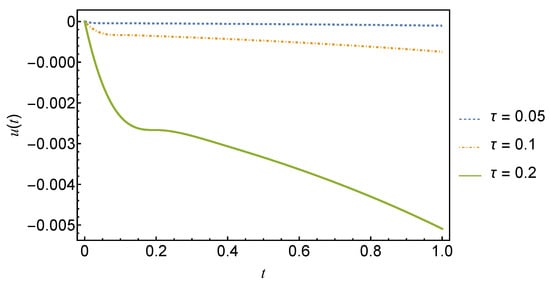
The delay differential equation

$$\frac{du\left(t\right)}{dt}=u(t-\tau ),\tau >0,$$

(146)

with initial condition

$$u\left(t\right)=\varphi \left(t\right)\mathrm{for}t\le 0,$$

(147)

has the solution

$$u\left(t\right)=\varphi (-\tau )\mathrm{dexp}(t+\tau ;\tau )+{\int }_0^{\tau }{\varphi }^{\prime }(t^{\prime }-\tau )\mathrm{dexp}(t+\tau -t^{\prime };\tau )d{t}^{\prime }.$$

(148)

To show this, we first verify that it is a solution to the equation. From Lemma 1, we have

$$\frac{d}{dt}\mathrm{dexp}(t+a;\tau )=\mathrm{dexp}(t+a-\tau ;\tau )$$

so that, given $u\left(t\right)$ in Equation (148), we have

$$\frac{du\left(t\right)}{dt}=\varphi (-\tau )\mathrm{dexp}(t;\tau )+{\int }_0^{\tau }{\varphi }^{\prime }(t^{\prime }-\tau )\mathrm{dexp}(t-t^{\prime };\tau )d{t}^{\prime }=u(t-\tau ).$$

It remains to show that the solution, Equation (148), matches the initial condition. First, we note that

$$\mathrm{dexp}(t;\tau )=\left\{\begin{array}{cc}0\hfill & t<0,\hfill \\ 1\hfill & 0\le t\le \tau ,\hfill \end{array}\right.$$

(149)

hence, $\mathrm{dexp}(t+\tau ;\tau )=1$ for $-\tau \le t\le 0$ and $\mathrm{dexp}(t+\tau -t^{\prime };\tau )=\Theta (t+\tau -t^{\prime })$ if $0\le t^{\prime }\le \tau$ and $-\tau \le t\le 0$. Thus, if $-\tau \le t\le 0$, we can rewrite Equation (148) as

$$u\left(t\right)=\varphi (-\tau )+{\int }_0^{\tau }{\varphi }^{\prime }(t^{\prime }-\tau )\Theta (t+\tau -t^{\prime })d{t}^{\prime }.$$

(150)

Clearly, the integral vanishes if $t^{\prime }>t+\tau$, so that

$$\begin{array}{cc}\hfill u\left(t\right)& =\varphi (-\tau )+{\int }_0^{t+\tau }{\varphi }^{\prime }(t^{\prime }-\tau )d{t}^{\prime }\hfill \end{array}$$

(151)

$$\begin{array}{cc}\hfill & =\varphi \left(t\right).\hfill \end{array}$$

(152)

In the special case with $\varphi \left(t\right)=1$, we recover $u\left(t\right)=\mathrm{dexp}(t+\tau ;\tau )$. The dynamics of the solution given by Equation (148) are illustrated in Figure 5 for various delays.

Figure 5. Plot of the solution, Equation (148), with $\varphi \left(t\right)=-t^2$ for delays $\tau =0.05,0.1,0.2$. The solid green line is for $\tau =0.2$ and the dashed blue and red lines are for $\tau =0.05$ and $\tau =0.1$, respectively.

We can readily construct more complicated equations that involve delay functions in their solutions. This is highlighted by the next example.

Example 8.

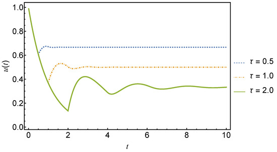
The delay differential equation

$$\frac{du\left(t\right)}{dt}=-au\left(t\right)+bu(t-\tau ),a,b\in \mathbb{R},\tau >0,$$

(153)

with the initial condition

$$u\left(t\right)=\left\{\begin{array}{cc}0\hfill & t<0,\hfill \\ 1\hfill & t=0,\hfill \end{array}\right.$$

(154)

has the solution

$$u\left(t\right)=e^{-at}\mathrm{dexp}(b{e}^{a\tau }t;b{e}^{a\tau }\tau ).$$

(155)

To show this, let $v\left(t\right)=e^{at}u\left(t\right)$, so that Equation (153) is consistent with

$$\frac{dv\left(t\right)}{dt}=b{e}^{a\tau }v(t-\tau ),$$

(156)

which has solution $\mathrm{dexp}(b{e}^{a\tau }t;b{e}^{a\tau }\tau )$, and the result then follows. The dynamics of the solution given by Equation (155) are illustrated in Figure 6 for various delays.

Figure 6. Plot of the solution, Equation (155), with $a=1.0$ and $b=1.0$ for delays $\tau =0.5,1.0,2.0$. The solid green line is for $\tau =2.0$ and the dashed blue and red lines are for $\tau =0.5$ and $\tau =1.0$, respectively.

The following theorem shows the more general utility of delay functions in representing solutions to delay differential equations.

Theorem 3.

If $f\left(x\right)$ permits a power series representation, Equation (4), with the jth derivative

$$\frac{d^j}{d{x}^j}f\left(x\right)=g\left(x\right),$$

(157)

then

$$\frac{d^j}{d{x}^j}\mathrm{df}(\lambda x;\lambda \sigma )={\lambda }^j\mathrm{dg}(\lambda (x-j\sigma );\lambda \sigma )+\sum _{k=0}^{j-1}\frac{k!a_k{\lambda }^k}{{\sigma }^{j-k}}{\delta }^{(j-1-k)}\left(\frac{x}{\sigma }-k\right),\frac{x}{\sigma }\in \mathbb{R},\lambda \in \mathbb{C},$$

(158)

where $\mathrm{df}(x;\sigma )$ is the corresponding delay function for $f\left(x\right)$, and $\mathrm{dg}(x;\sigma )$ is the corresponding delay function for $g\left(x\right)$.

Proof. 

Starting with the power series

$$f\left(x\right)=\sum _{n=0}^{+\infty }{a}_n{x}^n$$

(159)

and differentiating j times, we arrive at

$$\frac{d^j}{d{x}^j}f\left(x\right)=\sum _{n=0}^{+\infty }{a}_{n+j}{(n+1)}^{\overline{j}}{x}^n.$$

(160)

Hence, we now have

$$g\left(x\right)=\sum _{n=0}^{+\infty }{a}_{n+j}{(n+1)}^{\overline{j}}{x}^n.$$

(161)

From Equation (159), we identify the corresponding delay function

$$\mathrm{df}(x;\sigma )=\sum _{n=0}^{+\infty }{a}_n{(x-n\sigma )}^n\Theta \left(\frac{x}{\sigma }-n\right)$$

(162)

and then

$$\mathrm{df}(\lambda x;\lambda \sigma )=\sum _{n=0}^{+\infty }{a}_n{\lambda }^n{(x-n\sigma )}^n\Theta \left(\frac{x}{\sigma }-n\right).$$

(163)

Hence, differentiating Equation (163) j times, we obtain

$$\begin{array}{cc}\hfill \frac{d^j}{d{x}^j}\mathrm{df}(\lambda x;\lambda \sigma )& =\sum _{n=0}^{+\infty }{a}_{n+j}{\lambda }^{n+j}{(n+1)}^{\overline{j}}{(x-(n+j)\sigma )}^n\Theta \left(\frac{x}{\sigma }-n-j\right)\hfill \\ \hfill & +\sum _{k=0}^{j-1}\frac{k!a_k{\lambda }^k}{{\sigma }^{j-k}}{\delta }^{(j-1-k)}\left(\frac{x}{\sigma }-k\right).\hfill \end{array}$$

(164)

From Equation (161), we identify the corresponding delay function

$$\mathrm{dg}(x;\sigma )=\sum _{n=0}^{+\infty }{a}_{n+j}{(n+1)}^{\overline{j}}{(x-n\sigma )}^n\Theta \left(\frac{x}{\sigma }-n\right)$$

(165)

and then

$${\lambda }^j\mathrm{dg}(\lambda (x-j\sigma );\lambda \sigma )=\sum _{n=0}^{+\infty }{a}_{n+j}{\lambda }^{n+j}{(n+1)}^{\overline{j}}{(x-(n+j)\sigma )}^n\Theta \left(\frac{x}{\sigma }-n-j\right),$$

(166)

which matches the first sum on the right-hand side of Equation (164). □

Example 9.

Consider the logarithmic function $f\left(x\right)=\log (1+x)$ with derivative $g\left(x\right)=\frac{1}{1+x}$. Starting with the Taylor series for $f\left(x\right)$

$$\log (1+x)=\sum _{n=1}^{+\infty }{(-1)}^{n-1}\frac{x^n}{n},\left|x\right|<1,$$

(167)

we identify the corresponding delay function

$$\mathrm{df}(x;\sigma )=\sum _{n=1}^{+\infty }{(-1)}^{n-1}\frac{{(x-n\sigma )}^n}{n}\Theta \left(\frac{x}{\sigma }-n\right),\left|x\right|<1.$$

(168)

The Taylor series for $g\left(x\right)$ is

$$\frac{1}{1+x}=\sum _{n=0}^{+\infty }{(-1)}^n{x}^n,\left|x\right|<1,$$

(169)

with the corresponding delay function

$$\mathrm{dg}(x;\sigma )=\sum _{n=0}^{+\infty }{(-1)}^n{(x-n\sigma )}^n\Theta \left(\frac{x}{\sigma }-n\right),\left|x\right|<1.$$

(170)

From Theorem 3, we have

$$\begin{array}{cc}\hfill \frac{d}{dx}\mathrm{df}(x;\sigma )& =\mathrm{dg}(x-\sigma ;\sigma )+\frac{1}{\sigma }\delta \left(\frac{x}{\sigma }\right)\hfill \end{array}$$

(171)

$$\begin{array}{cc}\hfill & =\sum _{n=0}^{+\infty }{(-1)}^n\frac{{(x-\sigma -n\sigma )}^n}{n}\Theta \left(\frac{x-\sigma }{\sigma }-n\right)+\frac{1}{\sigma }\delta \left(\frac{x}{\sigma }\right),\left|x\right|<1.\hfill \end{array}$$

(172)

Corollary 5.

If $\mathrm{dy}(x;\sigma )$ is a delay function with

$$\mathrm{dy}(x;\sigma )=\sum _{n=0}^{+\infty }{a}_n{(x-n\sigma )}^n\Theta \left(\frac{x}{\sigma }-n\right),\frac{x}{\sigma }\in \mathbb{R},$$

(173)

then

$$\frac{d}{dx}\mathrm{dy}(f\left(x\right);\sigma )=f^{\prime }\left(x\right)\mathrm{dz}(f\left(x\right)-\sigma ;\sigma ),if\frac{f\left(x\right)}{\sigma }\in \mathbb{R}\setminus \left\{0\right\},$$

(174)

where $\mathrm{dz}(x;\sigma )$ is a delay function

$$\mathrm{dz}(x;\sigma )=\sum _{n=0}^{+\infty }{a}_{n+1}(n+1){(x-n\sigma )}^n\Theta \left(\frac{x}{\sigma }-n\right),\frac{x}{\sigma }\in \mathbb{R}.$$

(175)

Proof. 

This follows from an application of the chain rule and Theorem 3 with the identification

$$\frac{d}{dx}\mathrm{dy}(x;\sigma )=\mathrm{dz}(x-\sigma ;\sigma ).$$

(176)

□

Example 10.

Consider $\mathrm{dy}(x;\sigma )=\mathrm{dexp}(-x;-\sigma )$, then $a_n=\frac{{(-1)}^n}{n!}$ from which it follows that $a_{n+1}(n+1)=-a_n$ and $\mathrm{dz}(x;\sigma )=-\mathrm{dexp}(-x;-\sigma )$. Theorem 3 in this case yields

$$\frac{d}{dx}\mathrm{dexp}(-f\left(x\right);-\sigma )=-f^{\prime }\left(x\right)\left(\mathrm{dexp}(\sigma -f(x);-\sigma )\right).$$

(177)

Note that in the case of $f\left(x\right)=x$, we have

$$\frac{d}{dx}\mathrm{dexp}(-x;-\sigma )=-\mathrm{dexp}(\sigma -x;-\sigma ),$$

(178)

and in the case of $f\left(x\right)=\frac{x^2}{2}$, we have

$$\frac{d}{dx}\mathrm{dexp}\left(-\frac{x^2}{2};-\sigma \right)=-x\left(\mathrm{dexp}\left(\sigma -\frac{x^2}{2};-\sigma \right)\right).$$

(179)

It is worth comparing these results with the non-delay counterparts. We note that $\exp (-x)$ is the solution to the differential equation

$$\frac{dy\left(x\right)}{dx}=-y\left(x\right)$$

(180)

and from Equation (178), $\mathrm{dexp}(-x;-\sigma )$ is the solution to the delay differential equation

$$\frac{dy\left(x\right)}{dx}=-y(x-\sigma ).$$

(181)

We also note that $\exp \left(-\frac{x^2}{2}\right)$ is the solution to the differential equation

$$\frac{dy\left(x\right)}{dx}=-xy\left(x\right)$$

(182)

but from Equation (179), $\mathrm{dexp}\left(-\frac{x^2}{2};-\sigma \right)$ is not the solution to the delay differential equation

$$\frac{dy\left(x\right)}{dx}=-xy(x-\sigma ).$$

(183)

In the next example, we demonstrate the utility of Theorem 3 in solving first-order delay differential equations.

Example 11.

The delay differential equation

$$\frac{df\left(x\right)}{dx}+f(x-\sigma )=\frac{1}{\sigma }\delta \left(\frac{x}{\sigma }\right),\frac{x}{\sigma }\in \mathbb{R},$$

(184)

has a solution $\mathrm{dexp}(-x;-\sigma )$. This is easy to establish via the direct substitution of Definition 3 into the above equation with $\lambda =-1$. Alternatively, note that $\frac{df\left(x\right)}{dx}=f\left(x\right)$ has a solution $f\left(x\right)=\exp \left(x\right)$, and by using Theorem 3 with $g\left(x\right)=\exp \left(x\right)$ and $a_0=1$, we can write

$$\frac{d}{dx}\mathrm{dexp}(\lambda x;\lambda \sigma )=\lambda \mathrm{dexp}(\lambda (x-\sigma );\lambda \sigma )+\frac{1}{\sigma }\delta \left(\frac{x}{\sigma }\right).$$

(185)

If $\lambda =-1$ this identifies $\mathrm{dexp}(-x;-\sigma )$ as a solution to the delay differential equation, Equation (184). The solution can also be represented as a linear combination of Lambert W functions [10,23], and it can be generalized to include more general initial conditions [12] and systems of equations [11,12].

Using Theorem 3, we can solve higher-order delay differential equations, which we consider in the following example.

Example 12.

The delay differential equation

$$\frac{d^{2}f\left(x\right)}{d{x}^2}+f(x-2\sigma )=\frac{1}{{\sigma }^2}{\delta }^{\left(1\right)}\left(\frac{x}{\sigma }\right),\frac{x}{\sigma }\in \mathbb{R},$$

(186)

has a solution $\mathrm{dcos}(x;\sigma )$. This is easy to establish via direct substitution of Definition 4 into the above equation. Alternatively, note that $\frac{d^{2}f\left(x\right)}{d{x}^2}=-f\left(x\right)$ has a solution $f\left(x\right)=\cos \left(x\right)$, and by using Theorem 3 with $g\left(x\right)=-\cos \left(x\right)$, $a_0=1$, and $a_1=0$, we can write

$$\frac{d^2}{d{x}^2}\mathrm{dcos}(\lambda x;\lambda \sigma )=-{\lambda }^2\mathrm{dcos}(\lambda (x-2\sigma );\lambda \sigma )+\frac{1}{{\sigma }^2}{\delta }^{\left(1\right)}\left(\frac{x}{\sigma }\right).$$

(187)

If $\lambda =1$, this identifies $\mathrm{dcos}(x;\sigma )$ as a solution to the delay differential equation, Equation (186). We observe that $f\left(x\right)=\sin \left(x\right)$ is also a solution of $\frac{d^{2}f\left(x\right)}{d{x}^2}=-f\left(x\right)$ and by using Theorem 3 with $g\left(x\right)=-\sin \left(x\right)$, $a_0=0$, and $a_1=1$, we can write

$$\frac{d^2}{d{x}^2}\mathrm{dsin}(\lambda x;\lambda \sigma )=-{\lambda }^2\mathrm{dsin}(\lambda (x-2\sigma );\lambda \sigma )+\frac{\lambda }{\sigma }\delta \left(\frac{x}{\sigma }-1\right).$$

(188)

Interestingly, if $\lambda =1$, this identifies $\mathrm{dsin}(x;\sigma )$ as a solution of a separate delay differential equation

$$\frac{d^{2}f\left(x\right)}{d{x}^2}+f(x-2\sigma )=\frac{1}{\sigma }\delta \left(\frac{x}{\sigma }-1\right),\frac{x}{\sigma }\in \mathbb{R}.$$

(189)

The use of delay sine and cosine functions to represent solutions of systems of second-order differential delay equations with Cauchy initial conditions was explored in [13].

Corollary 6.

If $x\ne k\sigma$ with $k\in \mathbb{N}$ and $k<j$, then Equation (158) reduces to

$$\frac{d^j}{d{x}^j}\mathrm{df}(\lambda x;\lambda \sigma )={\lambda }^j\mathrm{dg}(\lambda (x-j\sigma );\lambda \sigma ),\frac{x}{\sigma }\in \mathbb{R},\lambda \in \mathbb{C}.$$

(190)

Proof. 

From Equation (158), we observe that the sum on the right-hand side vanishes for all $x\in \mathbb{R}$, except $x=k\sigma$ with $k\in \mathbb{N}$ and $k<j$. □

The next example highlights how delay function series expansions can solve specific linear delay differential equations.

Example 13.

Consider the delay differential equation

$$\frac{d^{2}y\left(x\right)}{d{x}^2}-\frac{dy(x-\sigma )}{dx}+y(x-2\sigma )=0,\frac{x}{\sigma }\in \mathbb{R}.$$

(191)

If $x\ne k\sigma$ for $k=0,1$, we can use Corollary 6 to seek a delay function series expansion solution to the form

$$y\left(x\right)=\sum _{n=0}^{+\infty }{a}_n{(x-n\sigma )}^n\Theta \left(\frac{x}{\sigma }-n\right)$$

(192)

by substituting this into the equation. It is straightforward to show that

$$y(x-2\sigma )=\sum _{n=0}^{+\infty }{a}_n{(x-(n+2)\sigma )}^n\Theta \left(\frac{x}{\sigma }-n-2\right)$$

(193)

and

$$\frac{d^{2}y\left(x\right)}{d{x}^2}=\sum _{n=0}^{+\infty }{a}_{n+2}(n+1)(n+2){(x-(n+2)\sigma )}^n\Theta \left(\frac{x}{\sigma }-n-2\right).$$

(194)

We also have

$$y(x-\sigma )=\sum _{n=0}^{+\infty }{a}_n{(x-(n+1)\sigma )}^n\Theta \left(\frac{x}{\sigma }-n-1\right)$$

(195)

and then

$$\frac{dy(x-\sigma )}{dx}=\sum _{n=0}^{+\infty }{a}_{n+1}(n+1){(x-(n+2)\sigma )}^n\Theta \left(\frac{x}{\sigma }-n-2\right).$$

(196)

We now substitute the delay series expansions from Equations (193), (194), and (196) into Equation (191) to arrive at

$$\sum _{n=0}^{+\infty }\left(a_{n+2}(n+1)(n+2)-a_{n+1}(n+1)+a_n\right){(x-(n+2)\sigma )}^n\Theta \left(\frac{x}{\sigma }-2-n\right)=0.$$

(197)

Thus, we require

$$a_{n+2}(n+1)(n+2)-a_{n+1}(n+1)+a_n=0.$$

(198)

If we choose initial conditions that are consistent with $a_0=1$ and $a_1=1$, then the recurrence relation can be solved in closed form, yielding

$$a_n=\frac{1}{3n!}\left(3\cos \left(\frac{n\pi }{3}\right)+\sqrt{3}\sin \left(\frac{n\pi }{3}\right)\right).$$

(199)

Finally, we have the solution

$$y\left(x\right)=\sum _{n=0}^{+\infty }\frac{1}{3n!}\left(3\cos \left(\frac{n\pi }{3}\right)+\sqrt{3}\sin \left(\frac{n\pi }{3}\right)\right){(x-n\sigma )}^n\Theta \left(\frac{x}{\sigma }-n\right).$$

(200)

We can generalize the example above by imposing an arbitrary initial condition.

Example 14.

The delay differential equation

$$\frac{d^{2}y\left(x\right)}{d{x}^2}-\frac{dy(x-\sigma )}{dx}+y(x-2\sigma )=0,\frac{x}{\sigma }\in \mathbb{R},$$

(201)

with initial condition

$$y\left(x\right)=\varphi \left(x\right)\mathrm{for}x\le 0,$$

(202)

has the solution

$$y\left(x\right)=\varphi (-\sigma )y_p(x+\sigma )+{\int }_0^{\sigma }{\varphi }^{\prime }(x^{\prime }-\sigma )y_p(x+\sigma -x^{\prime })d{x}^{\prime }$$

(203)

where $y_p\left(x\right)$ is the particular solution to the equation with the initial condition $y\left(x\right)=\Theta \left(x\right)$ for $x\le 0$ given by Equation (200), provided that $x\ne k\sigma$ for $k=0,1$. To show that this is a solution, let $y_p\left(x\right)=y_c\left(x\right)+y_s\left(x\right)$, where $y_c\left(x\right)$ and $y_s\left(x\right)$ are defined as

$$y_c\left(x\right)=\sum _{n=0}^{+\infty }\frac{1}{n!}\cos \left(\frac{n\pi }{3}\right){(x-n\sigma )}^n\Theta \left(\frac{x}{\sigma }-n\right)$$

(204)

and

$$y_s\left(x\right)=\sum _{n=0}^{+\infty }\frac{1}{n!}\frac{1}{\sqrt{3}}\sin \left(\frac{n\pi }{3}\right){(x-n\sigma )}^n\Theta \left(\frac{x}{\sigma }-n\right)$$

(205)

respectively. It is straightforward to show that

$$\frac{d{y}_p\left(x\right)}{dx}=y_c(x-\sigma )-y_s(x-\sigma )$$

(206)

and

$$\frac{d^2{y}_p\left(x\right)}{d{x}^2}=-2y_s(x-2\sigma )$$

(207)

so that, given $y\left(x\right)$ in Equation (203), we have

$$\begin{array}{cc}\hfill \frac{d^{2}y\left(x\right)}{d{x}^2}-\frac{dy(x-\sigma )}{dx}& =-\varphi (-\sigma )(y_c(x-\sigma )+y_s(x-\sigma ))\hfill \\ \hfill & -{\int }_0^{\sigma }{\varphi }^{\prime }(x^{\prime }-\sigma )(y_c(x-\sigma -x^{\prime })+y_s(x-\sigma -x^{\prime }))d{x}^{\prime }\hfill \end{array}$$

(208)

$$\begin{array}{cc}\hfill & =-\varphi (-\sigma )y_p(x-\sigma )-{\int }_0^{\sigma }{\varphi }^{\prime }(x^{\prime }-\sigma )y_p(x-\sigma -x^{\prime })d{x}^{\prime }\hfill \end{array}$$

(209)

$$\begin{array}{cc}\hfill & =-y(x-2\sigma ).\hfill \end{array}$$

(210)

Next, we verify that the solution, Equation (203), matches the initial condition. We note that $y_p\left(x\right)$, like $\mathrm{dexp}(x;\sigma )$, satisfies the properties

$$y_p\left(x\right)=\left\{\begin{array}{cc}0\hfill & x<0,\hfill \\ 1\hfill & 0\le x\le \sigma ,\hfill \end{array}\right.$$

(211)

hence $y_p\left(x\right)=\Theta \left(x\right)$ for $-\sigma \le x\le \sigma$. Therefore, if $-\sigma \le x\le 0$, we see that

$$\begin{array}{cc}\hfill y\left(x\right)& =\varphi (-\sigma )+{\int }_0^{\sigma }{\varphi }^{\prime }(x^{\prime }-\sigma )\Theta (x+\sigma -x^{\prime })d{x}^{\prime }\hfill \end{array}$$

(212)

$$\begin{array}{cc}\hfill & =\varphi (-\sigma )+{\int }_0^{x+\sigma }{\varphi }^{\prime }(x^{\prime }-\sigma )d{x}^{\prime }\hfill \end{array}$$

(213)

$$\begin{array}{cc}\hfill & =\varphi \left(x\right).\hfill \end{array}$$

(214)

The particular solution $y\left(x\right)=y_p\left(x\right)$ is recovered when $\varphi \left(x\right)=\Theta \left(x\right)$ for $x\le 0$.

Interestingly, the previous two examples are special cases of a more general theorem.

Theorem 4.

The mth-order linear delay differential equation of the form

$$c_m\frac{d^m}{d{x}^m}y\left(x\right)+c_{m-1}\frac{d^{m-1}}{d{x}^{m-1}}y(x-\sigma )+c_{m-2}\frac{d^{m-2}}{d{x}^{m-2}}y(x-2\sigma )+\cdots +c_{0}y(x-m\sigma )=0$$

(215)

where $c_j\in \mathbb{R}$, for all $j=0,1,\dots ,m$ has a delay series solution to the form

$$y\left(x\right)=\sum _{n=0}^{+\infty }{a}_n{(x-n\sigma )}^n\Theta \left(\frac{x}{\sigma }-n\right),\frac{x}{\sigma }\in \mathbb{R},$$

(216)

provided that $x\ne k\sigma$, for all $k=0,1,\dots ,m-1$.

Proof. 

Substituting Equation (216) into Equation (215) yields

$$\sum _{n=0}^{+\infty }\sum _{j=0}^m{c}_j{a}_{n+j}{(n+1)}^{\overline{j}}{(x-(n+m)\sigma )}^n\Theta \left(\frac{x}{\sigma }-m-n\right).$$

(217)

This requires

$$\sum _{j=0}^m{c}_j{a}_{n+j}{(n+1)}^{\overline{j}}=0,$$

(218)

which defines a linear homogeneous mth-order recurrence relation with polynomial coefficients to solve for the sequence, $a_n$. The initial terms of the sequence, $a_0,a_1,\dots ,a_{m-1}$, are defined by the initial conditions for Equation (215). □

6. Fractional-Order Delay Differential Equations

We now demonstrate the ability of fractional delay functions to solve various linear fractional-order delay differential equations. Although we focus on differential equations that involve the Caputo fractional derivative, it is possible to consider equations with alternative fractional derivatives. For readers interested in the history of fractional calculus, we refer them to the preface in the classic text on fractional differential equations by Podlubny [24].

Example 15.

For $0<\alpha <1$, the fractional-order delay differential equation

$${}^C{\mathcal{D}}_t^{\alpha }u\left(t\right)=-u(t-\tau ),\tau >0,$$

(219)

with initial condition

$$u\left(t\right)=\left\{\begin{array}{cc}0\hfill & t<0,\hfill \\ 1\hfill & t=0,\hfill \end{array}\right.$$

(220)

has the solution

$$u\left(t\right)={\mathrm{dE}}_{\alpha }^{-}(-t;-\tau )$$

(221)

where ${}^C{\mathcal{D}}_t^{\alpha }$ is a Caputo fractional derivative of order α [25],

$${}^C{\mathcal{D}}_t^{\alpha }u\left(t\right)=\frac{1}{\Gamma (1-\alpha )}{\int }_0^t\frac{u^{\prime }\left(t^{\prime }\right)}{{(t-t^{\prime })}^{\alpha }}d{t}^{\prime }.$$

(222)

To show this, we use Laplace transform methods, starting with the Laplace transform of the Caputo derivative

$${\mathcal{L}}_t\left[{}^C{\mathcal{D}}_t^{\alpha }u\left(t\right)\right]\left(s\right)=s^{\alpha }\widehat{u}\left(s\right)-s^{\alpha -1}u\left(0\right).$$

(223)

Consistent with the requirement, $u(t-\tau )=0$ if $t<\tau$, we introduce a Heaviside function on the right-hand side of the equation and take the Laplace transform using

$${\mathcal{L}}_t[u(t-\tau )\Theta (t-\tau )]\left(s\right)=e^{-s\tau }\widehat{u}\left(s\right).$$

(224)

The Laplace transform of Equation (219) then gives

$$s^{\alpha }\widehat{u}\left(s\right)-s^{\alpha -1}u\left(0\right)=-e^{-s\tau }\widehat{u}\left(s\right),$$

(225)

which we can solve for $\widehat{u}\left(s\right)$ with $u\left(0\right)=1$ to obtain

$$\widehat{u}\left(s\right)=\frac{1}{s+e^{-s\tau }{s}^{1-\alpha }}.$$

(226)

Recall from Table 1 that this is the Laplace transform of ${\mathrm{dE}}_{\alpha }^{-}(-t;-\tau )$. To show this, we can take the Laplace transform term-by-term in the definition of ${\mathrm{dE}}_{\alpha }^{-}(-t;-\tau )$ with

$${\mathcal{L}}_t\left[{(t-n\tau )}^{\alpha n}\Theta \left(\frac{t}{\tau }-n\right)\right]\left(s\right)=\Gamma (1+\alpha n)e^{-sn\tau }{s}^{-(1+\alpha n)}$$

(227)

and then sum over n using the series expansion $\frac{1}{1+x}={\sum }_{n=0}^{+\infty }{(-1)}^n{x}^n$. The solution to this example was essentially given in [26] but using different notations.

We can increase the complexity of the previous example through the addition of a function of time, $f\left(t\right)$, on the right-hand side of the equation.

Example 16.

For $0<\alpha <1$, the fractional-order delay differential equation

$${}^C{\mathcal{D}}_t^{\alpha }u\left(t\right)=-u(t-\tau )+f\left(t\right),\tau >0,$$

(228)

with initial condition

$$u\left(t\right)=\left\{\begin{array}{cc}0\hfill & t<0,\hfill \\ 1\hfill & t=0,\hfill \end{array}\right.$$

(229)

has the solution

$$u\left(t\right)={\mathrm{dE}}_{\alpha }^{-}(-t;-\tau )+{\int }_0^t{\mathrm{dE}}_{\alpha ,\alpha ,\alpha -1}^{-}(-(t-t^{\prime });-\tau )f\left(t^{\prime }\right)d{t}^{\prime }.$$

(230)

To show this, we can take a Laplace transform of the equation and solve for $\widehat{u}\left(s\right)$. We require the Laplace transform results

$${\mathcal{L}}_t\left[{\mathrm{dE}}_{\alpha }^{-}(-t;-\tau )\right]\left(s\right)=\frac{1}{s+e^{-s\tau }{s}^{1-\alpha }}$$

(231)

and

$${\mathcal{L}}_t\left[{\mathrm{dE}}_{\alpha ,\alpha ,\alpha -1}^{-}(-t;-\tau )\right]\left(s\right)=\frac{1}{s^{\alpha }+e^{-s\tau }},$$

(232)

which can be obtained from Table 1, together with the convolution rule for Laplace transforms to carry out the inverse Laplace transforms.

We can further generalize Example 15 by imposing an arbitrary initial condition.

Example 17.

For $0<\alpha <1$, the fractional-order delay differential equation

$${}^C{\mathcal{D}}_t^{\alpha }u\left(t\right)=u(t-\tau ),\tau >0,$$

(233)

with initial condition

$$u\left(t\right)=\varphi \left(t\right)\mathrm{for}t\le 0,$$

(234)

has the solution

$$u\left(t\right)=\varphi (-\tau ){\mathrm{dE}}_{\alpha }^{+}(t+\tau ;\tau )+{\int }_0^{\tau }{\varphi }^{\prime }(t^{\prime }-\tau ){\mathrm{dE}}_{\alpha }^{+}(t+\tau -t^{\prime };\tau )d{t}^{\prime }.$$

(235)

The study of fractional-order delay differential equations is a recent and rapidly growing field [14,15,16,26,27,28,29,30,31]. It is anticipated that special delay functions will facilitate the representation of solutions for these types of problems, more generally, and enable more direct comparisons with their non-delay counterparts.

7. Generalized Power Series Delay Functions

In the above, we developed definitions of delay functions based on power series expansions and fractional power series expansions. Clearly, it is possible to broaden this class of functions in many ways. Our primary focus above has been to define delay functions that could prove useful for finding solutions to delay differential equations. In the following, we consider delay functions based on an infinite series of powers of a delayed function. We refer to this class of functions as generalized power series delay functions. Our goal here has not been to be exhaustive in the identification of delay functions that can be used in solving delay differential equations, but to provide one of many possible generalizations.

Definition 13.

A generalized power series delay function of a real-valued function $h\left(x\right)$ with delay parameter σ is defined as

$$\mathrm{df}[h\left(x\right);\mu ](x;\sigma )=\sum _{n=0}^{+\infty }{a}_n{\left(\mu h(x-n\sigma )\right)}^n\Theta \left(\frac{x}{\sigma }-n\right),\frac{x}{\sigma },\mu \in \mathbb{R}.$$

(236)

Example 18.

If $\mu =-1$, $a_n=\frac{1}{\Gamma (\alpha n+1)}$ and $h\left(x\right)=x^{\alpha }$ for $0<\alpha <1$, then $\mathrm{df}[x^{\alpha };-1](x;\sigma )={\mathrm{dE}}_{\alpha }^{-}(-x;-\sigma )$. In the case that $\mu =1$, we would instead find that $\mathrm{df}[x^{\alpha };1](x;\sigma )={\mathrm{dE}}_{\alpha }^{+}(x;\sigma )$.

In previous sections, we showed that delay functions based on standard power series, and delay functions based on fractional power series, provided solutions to autonomous delay differential equations and autonomous fractional delay differential equations. In the following, we will show that we can use delay functions based on generalized power series, Equation (13), to provide solutions to certain delay differential equations with periodic coefficients.

Theorem 5.

The delay differential equation

$$\frac{dy\left(x\right)}{dx}=p\left(x\right)y(x-\sigma )+\frac{1}{\sigma }\delta \left(\frac{x}{\sigma }\right),\frac{x}{\sigma }\in \mathbb{R},$$

(237)

where $p\left(x\right)=p(x-\sigma )$ is continuous and periodic with period σ has a delay functional solution

$$y\left(x\right)=\sum _{n=0}^{+\infty }\frac{1}{n!}{\left(q(x-n\sigma )\right)}^n\Theta \left(\frac{x}{\sigma }-n\right),$$

(238)

where

$$q\left(x\right)={\int }_0^{x}p\left(s\right)ds.$$

(239)

Proof. 

Differentiating Equation (238) yields

$$\begin{array}{cc}\hfill \frac{dy\left(x\right)}{dx}& =\sum _{n=0}^{+\infty }\frac{1}{n!}np(x-n\sigma ){\left(q(x-n\sigma )\right)}^{n-1}\Theta \left(\frac{x}{\sigma }-n\right)\hfill \\ \hfill & +\sum _{n=0}^{+\infty }\frac{1}{n!}{\left(q(x-n\sigma )\right)}^n\frac{1}{\sigma }\delta \left(\frac{x}{\sigma }-n\right)\hfill \end{array}$$

(240)

$$\begin{array}{cc}\hfill & =\sum _{n=1}^{+\infty }\frac{1}{(n-1)!}p(x-n\sigma ){\left(q(x-n\sigma )\right)}^{n-1}\Theta \left(\frac{x}{\sigma }-n\right)+\frac{1}{\sigma }\delta \left(\frac{x}{\sigma }\right)\hfill \end{array}$$

(241)

$$\begin{array}{cc}\hfill & =\sum _{n=0}^{+\infty }\frac{1}{n!}p(x-\sigma -n\sigma ){\left(q(x-\sigma -n\sigma )\right)}^n\Theta \left(\frac{x-\sigma }{\sigma }-n\right)+\frac{1}{\sigma }\delta \left(\frac{x}{\sigma }\right),\hfill \end{array}$$

(242)

but since $p(x-\sigma -n\sigma )=p\left(x\right)$, this becomes

$$\begin{array}{cc}\hfill \frac{dy\left(x\right)}{dx}& =p\left(x\right)\sum _{n=0}^{+\infty }\frac{1}{n!}{\left(q(x-\sigma -n\sigma )\right)}^n\Theta \left(\frac{x-\sigma }{\sigma }-n\right)+\frac{1}{\sigma }\delta \left(\frac{x}{\sigma }\right)\hfill \end{array}$$

(243)

$$\begin{array}{cc}\hfill & =p\left(x\right)y(x-\sigma )+\frac{1}{\sigma }\delta \left(\frac{x}{\sigma }\right).\hfill \end{array}$$

(244)

□

In the corollary below, we show that if the periodic function $p\left(x\right)=p(x-\sigma )$ has a mean of zero, then the infinite sum solution, Equation (238), for Equation (237), can be simplified to a closed-form solution.

Corollary 7.

If $p\left(x\right)$ is a periodic function with period σ and a mean of zero, then the delay differential equation, Equation (5), has a closed-form solution

$$y\left(x\right)=\frac{\Gamma (1+\lfloor \frac{x}{\sigma }\rfloor ,q\left(x\right))}{\Gamma (1+\lfloor \frac{x}{\sigma }\rfloor )}{e}^{q\left(x\right)},\frac{x}{\sigma }\in \mathbb{R},$$

(245)

where $q\left(x\right)$, defined by Equation (239), is periodic with period σ, and

$$\Gamma (b,c)={\int }_c^{+\infty }{x}^{b-1}{e}^{-x}dx$$

(246)

denotes the upper incomplete gamma function.

Proof. 

We begin by showing that if $p\left(x\right)$ is periodic with period $\sigma$ and has a mean of zero, then $q\left(x\right)$, defined by Equation (239), is periodic with period $\sigma$. Note that if $p\left(x\right)$ is periodic with period $\sigma$, then from Equation (239), we can write

$$\begin{array}{cc}\hfill q\left(x\right)& ={\int }_0^{x}p(s+\sigma )ds\hfill \end{array}$$

(247)

$$\begin{array}{cc}\hfill & ={\int }_{\sigma }^{x+\sigma }p\left(r\right)dr.\hfill \end{array}$$

(248)

It then follows that

$$\begin{array}{cc}\hfill q(x-\sigma )& ={\int }_{\sigma }^{x}p\left(r\right)dr\hfill \end{array}$$

(249)

$$\begin{array}{cc}\hfill & ={\int }_0^{x}p\left(r\right)dr-{\int }_0^{\sigma }p\left(r\right)dr\hfill \end{array}$$

(250)

$$\begin{array}{cc}\hfill & =q\left(x\right)-{\int }_0^{\sigma }p\left(r\right)dr.\hfill \end{array}$$

(251)

But if $p\left(x\right)$ is periodic with period $\sigma$ and has a mean of zero, then

$${\int }_0^{\sigma }p\left(r\right)dr=0$$

(252)

so that $q\left(x\right)=q(x-\sigma )$ is periodic with period $\sigma$, and we can replace $q(x-n\sigma )$ with $q\left(x\right)$ in the solution to the delay differential equation from Theorem 5 to obtain

$$y\left(x\right)=\sum _{n=0}^{+\infty }\frac{1}{n!}{\left(q\left(x\right)\right)}^n\Theta \left(\frac{x}{\sigma }-n\right)$$

(253)

or equivalently

$$y\left(x\right)=\sum _{n=0}^{\lfloor \frac{x}{\sigma }\rfloor }\frac{1}{n!}{\left(q\left(x\right)\right)}^n,$$

(254)

which simplifies to give Equation (245) since

$$\sum _{n=0}^k\frac{x^n}{n!}=\frac{\Gamma (1+k,x)}{\Gamma (1+k)}{e}^x.$$

(255)

Note that the above result is simple to establish using Laplace transform methods. □

We demonstrate the utility of the previous theorem and corollary in the following final example.

Example 19.

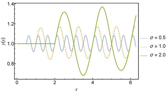
The delay differential equation

$$\frac{dy\left(x\right)}{dx}=\cos \left(\frac{2\pi x}{\sigma }\right)y(x-\sigma )+\frac{1}{\sigma }\delta \left(\frac{x}{\sigma }\right),\frac{x}{\sigma }\in \mathbb{R},$$

(256)

has the solution

$$y\left(x\right)=\sum _{n=0}^{+\infty }\frac{{\sigma }^n}{n!{\left(2\pi \right)}^n}{\sin }^n\left(\frac{2\pi x}{\sigma }\right)\Theta \left(\frac{x}{\sigma }-n\right),$$

(257)

which simplifies to the closed-form solution

$$y\left(x\right)=\frac{\Gamma (1+\lfloor \frac{x}{\sigma }\rfloor ,\frac{\sigma }{2\pi }\sin \left(\frac{2\pi x}{\sigma }\right))}{\Gamma (1+\lfloor \frac{x}{\sigma }\rfloor )}{e}^{\frac{\sigma }{2\pi }\sin \left(\frac{2\pi x}{\sigma }\right)}.$$

(258)

The dynamics of the solution given by Equation (258) are illustrated in Figure 7 for various delays.

Figure 7. Plot of the solution, Equation (258), for delays $\sigma =0.5,1.0,2.0$. The solid green line is for $\sigma =2.0$ and the dashed blue and red lines are for $\sigma =0.5$ and $\sigma =1.0$, respectively.

8. Summary

In the above, we provided a systematic approach to delay functions, defined as truncated power series or truncated fractional power series, characterized by a delay parameter $\sigma$, where the variable in the nth term of the series is delayed by $n\sigma$. Here, we concentrated on the properties of the functions over real variables. We provided their Laplace transform properties and demonstrated how the delay functions could be used to represent solutions of autonomous linear delay differential equations and autonomous linear delay fractional differential equations. Starting with the series expansion solution of an autonomous linear differential equation, we identified a corresponding delay series expansion as a solution of a corresponding autonomous linear delay differential equation. We then showed how general delay series expansions could be employed as trial solutions to construct solutions for arbitrary delay linear differential equations with constant coefficients. Finally, we considered more general delay functions based on truncated series expansions with delayed arguments in powers of general functions, $h\left(x\right)$, rather than powers of x or powers of $x^{\alpha }$.

This systematic approach to delay functions that we provide here should make them more accessible to a broader mathematics community, and bring further attention to important results that have already been made [11,12,13,14,15,16,26]. More generally, we hope that this publication will simplify modeling with delay differential equations and inspire others to extend research on novel delay functions and their properties.

References

- Abramowitz, M.; Stegun, I.A. Handbook of Mathematical Functions with Formulas, Graphs, and Mathematical Tables; NBS Applied Mathematics Series 55; National Bureau of Standards: Washington, DC, USA, 1964. [Google Scholar]
- Gorenflo, R.; Kilbas, A.A.; Mainardi, F.; Rogosin, S. Mittag-Leffler Functions, Related Topics and Applications, 2nd ed.; Springer: Berlin/Heidelberg, Germany, 2020. [Google Scholar] [CrossRef]
- Mainardi, F. Why the Mittag-Leffler function can be considered the Queen function of the fractional calculus? Entropy 2020, 22, 1359. [Google Scholar] [CrossRef] [PubMed]
- Erneux, T. Applied Delay Differential Equations; Springer: New York, NY, USA, 2009; Volume 3. [Google Scholar] [CrossRef]
- Rihan, F.A. Delay Differential Equations and Applications to Biology, 1st ed.; Springer: Singapore, 2021. [Google Scholar] [CrossRef]
- Kyrychko, Y.N.; Hogan, S.J. On the use of delay equations in engineering applications. J. Vib. Control 2010, 16, 943–960. [Google Scholar] [CrossRef]
- Yan, X.; Bauer, R.; Koch, G.; Schropp, J.; Perez Ruixo, J.J.; Krzyzanski, W. Delay differential equations based models in NONMEM. J. Pharmacokinet. Pharmacodyn. 2021, 48, 763–802. [Google Scholar] [CrossRef] [PubMed]
- Ramana Reddy, D.V.; Sen, A.; Johnston, G.L. Time delay induced death in coupled limit cycle oscillators. Phys. Rev. Lett. 1998, 80, 5109. [Google Scholar] [CrossRef]
- Beretta, E.; Kuang, Y. Geometric stability switch criteria in delay differential systems with delay dependent parameters. SIAM. J. Math. Anal. 2002, 33, 1144–1165. [Google Scholar] [CrossRef]
- Corless, R.M.; Gonnet, G.H.; Hare, D.E.G.; Jeffrey, D.J.; Knuth, D.E. On the LambertW function. Adv. Comput. Math. 1996, 5, 329–359. [Google Scholar] [CrossRef]
- Diblík, J.; Khusainov, D.Y. Reprersentation of solutions of linear discrete systems with constant coefficients and pure delay. Adv. Differ. Equ. 2006, 80825, 1–13. [Google Scholar] [CrossRef]
- Khusainov, D.Y.; Ivanov, A.F.; Shuklin, G.V. On a representation of solutions of linear delay systems. Differ. Equ. 2005, 41, 1054–1058. [Google Scholar] [CrossRef]
- Khusainov, D.Y.; Diblík, J.; Ruzickova, M.; Lukacova, J. Representation of a solution of the Cauchy problem for an oscillating system with pure delay. Nonlinear Oscil. 2008, 11, 276–285. [Google Scholar] [CrossRef]
- Li, M.; Wang, J.R. Exploring delayed Mittag-Leffler type matrix functions to study finite time stability of fractional delay differential equations. Appl. Math. Comput. 2018, 324, 254–265. [Google Scholar] [CrossRef]
- Li, M.; Wang, J.R. Finite time stability of fractional delay differential equations. Appl. Math. Lett. 2017, 64, 170–176. [Google Scholar] [CrossRef]
- Liu, L.; Dong, Q.; Li, G. Exact solutions of fractional oscillation systems with pure delay. Fract. Calc. Appl. Anal. 2022, 25, 1688–1712. [Google Scholar] [CrossRef]
- Mahmudov, N.I. Delayed perturbation of Mittag-Leffler functions and their applications to fractional linear delay differential equations. Math. Methods Appl. Sci. 2019, 42, 5489–5497. [Google Scholar] [CrossRef]
- Lighthill, M.J. Fourier Analysis and Generalised Functions; Cambridge University Press: Cambridge, UK, 1958. [Google Scholar]
- Angstmann, C.N.; Henry, B.I. Generalized fractional power series solutions for fractional differential equations. Appl. Math. Lett. 2020, 102, 106107. [Google Scholar] [CrossRef]
- El-Ajou, A.; Arqub, O.A.; Al-Zhour, Z.; Momani, S. New results on fractional power series: Theories and applications. Entropy 2013, 15, 5305–5323. [Google Scholar] [CrossRef]
- Rivero, M.; Rodríguez-Germá, L.; Trujillo, J.J. Linear fractional differential equations with variable coefficients. Appl. Math. Lett. 2008, 21, 892–897. [Google Scholar] [CrossRef][Green Version]
- Garrappa, R.; Rogosin, S.; Mainardi, F. On a generalized three-parameter Wright function of Le Roy type. Fract. Calc. Appl. Anal. 2017, 20, 1196–1215. [Google Scholar] [CrossRef]
- Pušenjak, R. Application of Lambert Functions in Control of Production Systems with Delay. Int. J. Eng. Sci. 2017, 6, 28–38. [Google Scholar] [CrossRef]
- Podlubny, I. Fractional Differential Equations: An Introduction to Fractional Derivatives, Fractional Differential Equations, to Methods of Their Solution and Some of Their Applications; Science and Engineering; Academic Press: Cambridge, MA, USA, 1999; Volume 198. [Google Scholar]
- Li, C.; Qian, D.; Chen, Y. On Riemann-Liouville and Caputo Derivatives. Discrete Dyn. Nat. Soc. 2011, 2011, 562494. [Google Scholar] [CrossRef]
- Garrappa, R.; Kaslik, E. On initial conditions for fractional delay differential equations. Commun. Nonlinear Sci. Numer. Simul. 2020, 90, 105359. [Google Scholar] [CrossRef]
- Cermák, J.; Kisela, T.; Nechvátal, L. The Lambert function method in qualitative analysis of fractional delay differential equations. Fract. Calc. Appl. Anal. 2023, 26, 1545–1565. [Google Scholar] [CrossRef]
- Jhinga, A.; Daftardar-Gejji, V. A new numerical method for solving fractional delay differential equations. J. Comput. Appl. Math. 2019, 38, 166. [Google Scholar] [CrossRef]
- Pan, R; Fan, Z. Analyses of solutions of Riemann-Liouville fractional oscillatory differential equations with pure delay. Math. Meth. Appl. Sci. 2023, 46, 10450–10464. [Google Scholar] [CrossRef]
- Polyanin, A.D.; Sorokin, V.G. Reductions and Exact Solutions of Nonlinear Wave-Type PDEs with Proportional and More Complex Delays. Mathematics 2023, 11, 516. [Google Scholar] [CrossRef]
- Singh, H. Numerical simulation for fractional delay differential equations. Int. J. Dyn. Control 2021, 9, 463–474. [Google Scholar] [CrossRef]
Disclaimer/Publisher’s Note: The statements, opinions and data contained in all publications are solely those of the individual author(s) and contributor(s) and not of MDPI and/or the editor(s). MDPI and/or the editor(s) disclaim responsibility for any injury to people or property resulting from any ideas, methods, instructions or products referred to in the content. |
© 2023 by the authors. Licensee MDPI, Basel, Switzerland. This article is an open access article distributed under the terms and conditions of the Creative Commons Attribution (CC BY) license (https://creativecommons.org/licenses/by/4.0/).