Mathematical Modeling of COVID-19 Dynamics under Two Vaccination Doses and Delay Effects

Abstract

The aim of this paper is to investigate the qualitative behavior of the COVID-19 pandemic under an initial vaccination program. We constructed a mathematical model based on a nonlinear system of delayed differential equations. The time delay represents the time that the vaccine takes to provide immune protection against SARS-CoV-2. We investigate the impact of transmission rates, vaccination, and time delay on the dynamics of the constructed system. The model was developed for the beginning of the implementation of vaccination programs to control the COVID-19 pandemic. We perform a stability analysis at the equilibrium points and show, using methods of stability analysis for delayed systems, that the system undergoes a Hopf bifurcation. The theoretical results reveal that under some conditions related to the values of the parameters and the basic reproduction number, the system approaches the disease-free equilibrium point, but if the basic reproduction number is larger than one, the system approaches endemic equilibrium and SARS-CoV-2 cannot be eradicated. Numerical examples corroborate the theoretical results and the methodology. Finally, conclusions and discussions about the results are presented.

1. Introduction

Coronavirus disease 2019 (COVID-19) is a respiratory illness caused by severe acute respiratory syndrome coronavirus 2 (SARS-CoV-2). SARS-CoV-2 moved rapidly around the world since it was first identified in Wuhan, China. The world has been suffering one of the worst pandemics in history, and how it will end is unclear at this time. Vaccination programs to control the spread of SARS-CoV-2 started at the very end of 2020 in a few countries [1,2]. Then, during 2021, more countries were able to implement vaccination programs. The vaccines worked well for the SARS-CoV-2 variants that were circulating at the beginning of the pandemic and mostly during 2021. However, in 2022, the efficacy of the vaccines has decreased due to the appearance of new SARS-CoV-2 variants and the effect of immune escape [3,4,5,6,7,8].

Many mathematical models have been used to study biological systems [9]. There are many dynamical systems connected to biology phenomena that are described by PDEs that involve dissipation actions [10,11]. In particular, some of them have been implemented for COVID-19 pandemic dynamics with spatial effects [12,13]. Some models have been used to investigate the impact of vaccines on the dynamics of the pandemic [2,14,15,16,17,18]. In addition, a few of these models have included and analyzed the effect of time delays on the pandemic dynamics [19,20,21,22,23,24,25,26]. For example, in [19], the authors proposed a model with a time delay in order to take into account the delay before an exposed individual could become infected. Other work is presented in [21], where an SEIR model with a time delay was used to study the COVID-19 pandemic. In [23], the authors presented a mathematical model based on a set of coupled delay differential equations with extensive delays, in order to estimate the incubation, recovery, and decease periods of COVID-19.

Different models have focused on different stages of the COVID-19 pandemic. Some models were used in the investigation of the period before vaccines were available [25,26,27,28,29,30,31,32,33,34]. Others focused on the beginning of vaccine availability. These models, however, are not applicable to the current situation where there are very different new SARS-CoV-2 variants and where booster vaccination programs have been implemented. For instance, factors such as variant competition, immune escape features, and cross-immunity are not present in many of the models developed at the beginning of the COVID-19 pandemic.

In this work, we design a mathematical model to study the impact of transmission rates, vaccination, and time delays on the dynamics of the COVID-19 pandemic. The model was created for the stage in which the vaccination programs were just starting. We use mathematical tools of dynamical systems and particularly from mathematical epidemiology for our aims. It has been shown that mathematical models, together with computational analysis techniques, have become important aids in testing hypotheses and analyzing the impact of different factors on infectious disease processes.

Many mathematical models that deal with infectious diseases rely on systems of differential equations to represent the dynamics of the disease at different levels, such as within-host and between hosts [16,18,35,36,37]. For some epidemic scenarios, it is suitable from a realistic viewpoint to include time delays into the models. Thus, to reflect dynamic behaviors more realistically, it is reasonable to rely on differential equations with time delays [26]. In this order of ideas, we use an SVEIR (susceptible, vaccinated, latent, infected, and recovered)-type mathematical epidemiological model to represent the dynamics of the COVID-19 pandemic for the beginning of the vaccination stage. The mathematical model developed includes the application of a vaccine that requires two doses and two mutually exclusive vaccinated subpopulations. The first subpopulation comprises individuals who have received only one dose, and the second one is those who have received two doses. The mathematical model constructed is based on a system of delay differential equations with a discrete time delay, where the inclusion of the time delay allows us to take into account that the vaccine does not provide immune protection instantaneously [22]. In addition, the model takes into account the possibility that individuals have only had one dose of the vaccine [1,15,22,38,39,40].

We begin the study of the time-delayed model by first obtaining the disease-free equilibrium point. Then, we find the basic reproduction number ${\mathcal{R}}_0$ using the next-generation matrix method [41]. Then, we find the unique endemic equilibrium point and we investigate the stability of the disease-free and the endemic equilibrium points. We also find the conditions for the system to show a Hopf bifurcation. Finally, with the appropriate choice of parameters, some numerical simulations are presented to check the effectiveness of the theoretical results obtained using nonstandard stable numerical schemes.

The organization of this paper is as follows: In Section 2 we construct and present the mathematical model. In Section 3 we study the existence and uniqueness, and positivity of the solution. The stability of the equilibrium points and the computation of the basic reproduction number ${\mathcal{R}}_0$ are presented in Section 4. In Section 5, the numerical simulations of the mathematical model are presented. Section 6 is devoted to conclusions.

2. Construction of the Mathematical Model

The study population is divided into several subpopulations. $S\left(t\right)$ denotes the population susceptible to the virus. If a susceptible individual comes into contact with an infectious individual and becomes infected, it transits to the latent population $E\left(t\right)$ as soon as the incubation period of the virus elapses and there is no transmissibility of the virus. When they can transmit the virus and show manifestations of the disease, we represent them as infectious $I\left(t\right)$, or if they infect without manifestations of the virus, we call them asymptomatic $A\left(t\right).$ With the variable $H\left(t\right)$ we denote hospitalized individuals, and in this model we assume that hospitalized individuals $H\left(t\right)$ cannot transmit the virus, assuming that conditions in hospitals are safe with respect to virus transmission. We denote with $V_1\left(t\right)$ and $V_2\left(t\right)$ the populations of susceptibles vaccinated for the first time and the individuals who are vaccinated and receive a dose for the second time, respectively. Now, with the variable $R\left(t\right)$ we denote the recovered population. We also assume that only susceptible individuals $S\left(t\right)$ are those who can be vaccinated and obviously those who have received the first dose of vaccination $V_1\left(t\right)$. This assumption may seem debatable, but in view of the risks involved in receiving vaccination while latent, infected, asymptomatic, or hospitalized, the viral load would increase in these populations and the consequences could be unfavorable on the health of the patients.

Thus, using the law of conservation of population and the law of mass action, the following equations are obtained:

• The change in $S\left(t\right)$ at time t is given by the inflow of new susceptibles $\Lambda$ and outflow of a proportion of first-dose vaccines at a rate ${\nu }_1$ of the form ${\nu }_{1}S(t-\tau ),$ the proportion infected due to the force of infection given by $\left({\beta }_{I}I\left(t\right)+{\beta }_{A}A\left(t\right)\right)S\left(t\right)$, and the proportion of deaths naturally by the death rate which is $dS\left(t\right).$ It follows that

  $$\dot{S}\left(t\right)=\mathrm{\Lambda }-dS\left(t\right)-({\beta }_{I}I\left(t\right)+{\beta }_{A}A\left(t\right))S\left(t\right)-{\nu }_{1}S(t-\tau ).$$
• The variation of $V_1\left(t\right)$ is given by the inflow of susceptibles vaccinated with the first dose ${\nu }_{1}S(t-\tau )$ and the outflow of the proportion of first-time vaccinees when there is the interaction with the force of infection ${\epsilon }_1\left({\beta }_{I}I\left(t\right)+{\beta }_{A}A\left(t\right)\right)V_1\left(t\right)$, plus the proportion of those vaccinated with the second dose ${\nu }_2{V}_1(t-\tau )$, and, in addition, those vaccinated who die naturally at a rate d. One obtains

  $${\dot{V}}_1\left(t\right)={\nu }_{1}S(t-\tau )-{ϵ}_1({\beta }_{I}I\left(t\right)+{\beta }_{A}A\left(t\right))V_1\left(t\right)-{\nu }_2{V}_1(t-\tau )-d{V}_1\left(t\right).$$
• The variation of $V_2\left(t\right)$ will consist of the entry of those vaccinated with the second dose ${\nu }_2{V}_1(t-\tau )$ and the exit of a proportion of individuals who have been given the second dose but become infected due to interaction with the force of infection ${\epsilon }_2\left({\beta }_{I}I\left(t\right)+{\beta }_{A}A\left(t\right)\right)V_2\left(t\right)$ and exit, and, also, people die naturally at a rate d. Thus, we obtain the equation

  $${\dot{V}}_2\left(t\right)={\nu }_2{V}_1(t-\tau )-{ϵ}_2({\beta }_{I}I\left(t\right)+{\beta }_{A}A\left(t\right))V_2\left(t\right)-d{V}_2\left(t\right).$$
• On the other hand, the variation of $E\left(t\right)$ is given by the inflow of new infectees which is represented by the expression

  $$\left({\beta }_{I}I\left(t\right)+{\beta }_{A}A\left(t\right)\right)\left(S\left(t\right)+{ϵ}_1{V}_1\left(t\right)+{ϵ}_2{V}_2\left(t\right)\right),$$

  while the outflow is given by individuals who transition to symptomatic or asymptomatic infectious stages in which they can transmit SARS-CoV-2 virus to others. The latent population transits to the infectious classes represented by the expression $\alpha E\left(t\right)$ and another part of latents that die naturally at a rate d. In conclusion, we obtain the equation

  $$\dot{E}\left(t\right)=({\beta }_{I}I\left(t\right)+{\beta }_{A}A\left(t\right))(S\left(t\right)+{ϵ}_1{V}_1\left(t\right)+{ϵ}_2{V}_2\left(t\right))-(d+\alpha )E\left(t\right).$$
• Variations of $I\left(t\right)$ and $A\left(t\right)$, $\dot{I}\left(t\right)$, and $\dot{A}\left(t\right)$, respectively, will first consist of individuals who are infected and initially remain in the latent stage E for a certain time with mean $\alpha$, and a proportion a of latent individuals enter the asymptomatic class $A\left(t\right)$ in a proportion $a\alpha E\left(t\right)$. The remaining proportion $(1-a)$ of latent individuals develop the symptoms of the disease and pass into the infected class $I\left(t\right)$ in a proportion of $(1-a)\alpha E\left(t\right)$. The population in the asymptomatic class $A\left(t\right)$ transits at a rate $\gamma$ to the recovered class $R\left(t\right)$, that is, the factor $\gamma A\left(t\right)$ leaves and enters $R\left(t\right)$. Similarly, infected persons I can pass into the recovered class R at a rate $\gamma$ in a proportion $\gamma I\left(t\right)$ and enter $R\left(t\right)$. Now, a part of the infected persons I can pass into the hospitalized class H at a rate h in a factor $hI\left(t\right)$. In addition, it is possible that infected $I\left(t\right)$ and asymptomatic $A\left(t\right)$ die naturally at a rate d. Thus, we obtain the equations

  $$\dot{A}\left(t\right)=a\alpha E\left(t\right)-(d+\gamma )A\left(t\right),\mathrm{and}$$

  $$\dot{I}\left(t\right)=(1-a)\alpha E\left(t\right)-(d+h+\gamma )I\left(t\right).$$
• The variations of $H\left(t\right)$ and $R\left(t\right)$, $\dot{H}\left(t\right)$, and $\dot{R}\left(t\right)$, respectively, are given by the transition to class H of class I with a factor $hI\left(t\right)$ of infected individuals who are hospitalized. The $\gamma I\left(t\right)$ and $\gamma A\left(t\right)$ arefactors of infected and asymptomatic individuals who recover enter the class R, that is, with a factor $\gamma \left(I\right(t)+A(t\left)\right)$. Persons of class H hospitalized die from the virus at a rate $\delta$, that is, they come out with a factor of $\delta H$, as well as the recovery of a percentage of those hospitalized at a rate $\rho$, that is, they enter the class R with a factor $\rho H$. In addition, it is possible that they die naturally hospitalized $H\left(t\right)$ and recovered $R\left(t\right)$ at a rate d. From all of the above, the equations are

  $$\dot{H}\left(t\right)=hI\left(t\right)-(d+\delta +\rho )H\left(t\right),\mathrm{and}$$

  $$\dot{R}\left(t\right)=\gamma (I\left(t\right)+A\left(t\right))+\rho H\left(t\right)-dR\left(t\right).$$

The flows between the interacting subpopulations can be seen in Figure 1. The above equations can be rewritten as the following system:

$$\dot{Y}\left(t\right)=f\left(t,Y\left(t\right)\right),t\in [0,\infty ),$$

(1)

where $Y\left(t\right)={\left(S\left(t\right),V_1\left(t\right),V_2\left(t\right),E\left(t\right),A\left(t\right),I\left(t\right),H\left(t\right),R\left(t\right)\right)}^T,$ and

$$f\left(t,Y\left(t\right)\right)=\left(\begin{array}{c}\Lambda -dS\left(t\right)-({\beta }_{I}I\left(t\right)+{\beta }_{A}A\left(t\right))S\left(t\right)-{\nu }_{1}S(t-\tau )\\ {\nu }_{1}S(t-\tau )-{ϵ}_1({\beta }_{I}I\left(t\right)+{\beta }_{A}A\left(t\right))V_1\left(t\right)-{\nu }_2{V}_1(t-\tau )-d{V}_1\left(t\right)\\ {\nu }_2{V}_1(t-\tau )-{ϵ}_2({\beta }_{I}I\left(t\right)+{\beta }_{A}A\left(t\right))V_2\left(t\right)-d{V}_2\left(t\right)\\ ({\beta }_{I}I\left(t\right)+{\beta }_{A}A\left(t\right))(S\left(t\right)+{ϵ}_1{V}_1\left(t\right)+{ϵ}_2{V}_2\left(t\right))-(d+\alpha )E\left(t\right)\\ a\alpha E\left(t\right)-(d+\gamma )A\left(t\right)\\ (1-a)\alpha E\left(t\right)-(d+h+\gamma )I\left(t\right)\\ hI\left(t\right)-(d+\delta +\rho )H\left(t\right)\\ \gamma \left(I\right(t)+A(t\left)\right)+\rho H\left(t\right)-dR\left(t\right)\end{array}\right),$$

where $t\in [0,\infty )$, and with initial conditions given by

$$\begin{array}{cc}\hfill & S\left(\theta \right)={\zeta }_1\left(\theta \right)>0,V_1\left(\theta \right)={\zeta }_2\left(\theta \right)>0,V_2\left(\theta \right)={\zeta }_3\left(\theta \right)\ge 0,E\left(\theta \right)={\zeta }_4\left(\theta \right)\ge 0,\hfill \\ \hfill & A\left(\theta \right)={\zeta }_5\left(\theta \right)\ge 0,I\left(\theta \right)={\zeta }_6\left(\theta \right)\ge 0,H\left(\theta \right)={\zeta }_7\left(\theta \right)\ge 0,R\left(\theta \right)={\zeta }_8\left(\theta \right)\ge 0,\hfill \end{array}$$

for $\theta \in [-\tau ,0]$ with ${\zeta }_i\left(\theta \right),i=1,\dots ,8$ continuous functions defined from the interval $[-\tau ,0]$ to ${\mathbb{R}}_{+}$ and with norm $\parallel {\zeta }_i\parallel =\underset{-\tau \le \theta \le 0}{sup}\left|{\zeta }_i\left(\theta \right)\right|,i=1,\dots ,8.$ Let $b>0$ and $\mathcal{S}=\mathcal{C}\left([-\tau ,b],{\mathbb{R}}_{+}^8\right)$ be the Banach space of continuous functions defined on the interval $[-\tau ,b]$ to ${\mathbb{R}}_{+}^8$ with the norm

$$\parallel x\parallel =\underset{-\tau \le \theta \le b}{sup}\parallel x\left(\theta \right)\parallel ,x\in \mathcal{S},$$

where $\parallel x\left(\theta \right)\parallel ={\displaystyle \sum _{i=1}^8}\left|x_i\left(\theta \right)\right|,$ [42].

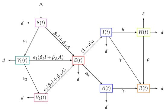
Figure 1. Flow diagram of the transit of the subpopulations over time of the model (1).

To analyze the dynamics of the solutions of system (1), we assume that

$$N\left(t\right)=S\left(t\right)+E\left(t\right)+I\left(t\right)+A\left(t\right)+H\left(t\right)+R\left(t\right)+V_1\left(t\right)+V_2\left(t\right),$$

(2)

and the initial values are given by

$$\begin{array}{cc}\hfill & S\left(0\right)=S_0>0,V_1\left(0\right)=V_{1,0}\ge 0,V_2\left(0\right)=V_{2,0}\ge 0,E\left(0\right)=E_0\ge 0,\hfill \\ \hfill & A\left(0\right)=A_0\ge 0,I\left(0\right)=I_0\ge 0,R\left(0\right)=R_0\ge 0,H\left(0\right)=H_0\ge 0;\hfill \end{array}$$

(3)

moreover,

$$\begin{array}{c}\hfill S_0={\zeta }_1\left(0\right)and{V}_{1,0}={\zeta }_2\left(0\right)\end{array}$$

(4)

satisfy the compatibility conditions.

In this model, two vaccination rates, ${\nu }_1$ and ${\nu }_2$, are considered for the populations $S\left(t\right)$ and $V_1\left(t\right)$, respectively, such that ${\nu }_2<{\nu }_1$, since the second dose has less demand than the first one. We are interested in studying the impact of vaccination rates and vaccine efficacies on the vaccination strategy [2,43,44]. For example, according to studies by Elisabeth Mahase [45], the Pfizer-BioNTech vaccine reached an effectiveness of 52% after the first dose $({\epsilon }_1=0.52)$ and 95% after the second dose $({\epsilon }_2=0.95)$. It is important to highlight that despite the plans made by health institutions regarding vaccination, there are many uncertainties present in the logistics. Therefore, here, we consider two different vaccination rates in this study.

Regarding the parameters ${\beta }_A$ and ${\beta }_I$, which represent the transmission rate between A and S and the transmission rate between I and S, respectively, we vary them due to the uncertainty of these rates. For instance, in [46], the authors concluded that asymptomatic carriers have a higher viral load and, taking into account that asymptomatic carriers may have more physical contacts, it is possible to assume that ${\beta }_A>{\beta }_I$. However, there are a variety of results for each region or country, as can be seen in [47,48,49,50,51].

3. Existence and Uniqueness of the Model Solution

Here, we prove the existence and uniqueness of the solution of the model (1). We start using the following theorem,

Theorem 1 

(Theorem 2.2. [42]). Suppose Ω is an open set in $\mathbb{R}\times \mathcal{S}$, $f:\Omega \to {\mathbb{R}}^n$ is continuous, and $f(t,\varphi )$ is Lipschitzian in ϕ, on every compact set in Ω. If $(\sigma ,\varphi )\in \Omega$, then there exists a unique solution of system (1) with initial value ϕ in σ.

To prove the existence of the solution through a point $(\sigma ,\varphi )\in [0,\infty )\times \mathcal{S}$, we consider a $b>0$ and all functions x on $[\sigma -\tau ,\sigma +b]$ which are continuous and coincide with $\varphi$ on $[\sigma -\tau ,\sigma ].$

Theorem 2.

Consider f as in (1) and suppose that Ω is an open set in $\mathbb{R}\times \mathcal{S},$ such that $f:\Omega \to {\mathbb{R}}^n$ is continuous. Let $C_0=[0,b]\times \mathcal{S}$ for every compact set in Ω. If $f(t,\varphi )$ is Lipschitzian in ϕ, then there exists a unique solution of system (1) with initial value ϕ in 0.

Proof.

In particular for $\sigma =0,$ we have that the function $f:[0,\infty )\times \mathcal{S}\to {\mathbb{R}}^8$ given by (1) is continuous and satisfies the local Lipschitz condition. Indeed, for ${\varphi }_1,{\varphi }_2\in C_0,$

$${\varphi }_1\left(t\right)={\left(S^1\left(t\right),V_1^1\left(t\right),V_2^1\left(t\right),E^1\left(t\right),A^1\left(t\right),I^1\left(t\right),H^1\left(t\right),R^1\left(t\right)\right)}^T,$$

$${\varphi }_2\left(t\right)={\left(S^2\left(t\right),V_1^2\left(t\right),V_2^2\left(t\right),E^2\left(t\right),A^2\left(t\right),I^2\left(t\right),H^2\left(t\right),R^2\left(t\right)\right)}^T,$$

and for $t\in [-\tau ,b]$, one obtains

$$\begin{array}{cc}\hfill \parallel f\left(t,{\varphi }_2\right)-f\left(t,{\varphi }_1\right)\parallel & \le M\underset{t\in [-\tau ,b]}{sup}\{\left|S^2\left(t\right)-S^1\left(t\right)\right|+\left|V_1^2\left(t\right)-V_1^1\left(t\right)\right|+\left|V_2^2\left(t\right)-V_2^1\left(t\right)\right|\hfill \\ & +\left|E^2\left(t\right)-E^1\left(t\right)\right|+\left|A^2\left(t\right)-A^1\left(t\right)\right|+\left|I^2\left(t\right)-I^1\left(t\right)\right|+\left|H^2\left(t\right)-H^1\left(t\right)\right|\hfill \\ & +\left|R^2\left(t\right)-R^1\left(t\right)\right|\}=M\parallel {\varphi }_2-{\varphi }_1\parallel ,\hfill \end{array}$$

i.e.,

$$\parallel f\left(t,{\varphi }_2\right)-f\left(t,{\varphi }_1\right)\parallel \le M\parallel {\varphi }_2-{\varphi }_1\parallel ,$$

where

$$\begin{array}{cc}\hfill M& =\underset{t\in [-\tau ,b]}{max}\{d+2{\nu }_1+2|g_1\left(t\right)|,d+2{\nu }_2+2{\epsilon }_1|g_1\left(t\right)|,d+2{\epsilon }_2\left|g_1\left(t\right)\right|,d+2\alpha ,\hfill \\ \hfill & d+2\gamma +2{\beta }_A|g_2\left(t\right)|,d+2\gamma +2h+2{\beta }_I\left|g_2\left(t\right)\right|,d+\delta +\rho +\gamma ,d\},\hfill \end{array}$$

$$g_1\left(t\right)={\beta }_I{I}^2\left(t\right)+{\beta }_A{A}^2\left(t\right)\mathrm{and}{g}_2\left(t\right)=S^1\left(t\right)+{\epsilon }_1{V}_1^1\left(t\right)+{\epsilon }_2{V}_2^1\left(t\right).$$

Then $f\left(t,Y\left(t\right)\right)$ given by (1) is local Lipschitzian. Applying Theorem 1, it follows the conclusion of the theorem. □

3.1. Positivity of Model Solutions

Since system (1) is a population model, the solutions must be positive. We reached the following result.

Theorem 3.

The model (1) with initial conditions given by (3) has positive solutions

$$\left(S\left(t\right),V_1\left(t\right),V_2\left(t\right),E\left(t\right),A\left(t\right),I\left(t\right),H\left(t\right),R\left(t\right)\right)$$

for all $t\in [0,\infty ),$ when $\tau \to 0^{+}.$

Proof.

For the proposed model, we have the following:

• $S\left(t\right)>0$, $\forall t>0$. Suppose that there exists $t_1>0$ such that $\dot{S}\left(t_1\right)\le 0$, $S\left(t_1\right)=0$ and $S\left(t\right)>0$ for all $t\in [0,t_1)$, so that

  $$\begin{array}{cc}\hfill \dot{S}\left(t_1\right)& =\Lambda -dS\left(t_1\right)-\left({\beta }_{I}I\left(t_1\right)+{\beta }_{A}A\left(t_1\right)\right)S\left(t_1\right)-{\nu }_{1}S(t_1-\tau )\hfill \\ \hfill \dot{S}\left(t_1\right)& =\Lambda -{\nu }_{1}S(t_1-\tau ),\hfill \end{array}$$

  for all $\tau >0$. Using the continuity of the solutions, it follows that $\Lambda -{\nu }_{1}S(t_1-\tau )\to \Lambda$ as $\tau \to 0,$ therefore we have a contradiction. Thus, $S\left(t\right)>0$ for all $t>0$. In the same way, it is verified that $V_1\left(t\right)>0,$$V_2\left(t\right)>0$, $\forall t>0$.
• $E\left(t\right),A\left(t\right),I\left(t\right)>0$$\forall t>0$. To show that $E\left(t\right)>0$ for all $t>0$, let us reason by contradiction. We assume that there exists $t_4>0$ such that $\dot{E}\left(t_4\right)\le 0$, $E\left(t_4\right)=0$ and $E\left(t\right)>0$ for all $t\in [0,t_4)$. Thus,

  $$\begin{array}{cc}\hfill \dot{E}\left(t_4\right)& =({\beta }_{I}I\left(t_4\right)+{\beta }_{A}A\left(t_4\right))(S\left(t_4\right)+{ϵ}_1{V}_1\left(t_4\right)+{ϵ}_2{V}_2\left(t_4\right))-(d+\alpha )E\left(t_4\right)\hfill \\ \hfill \dot{E}\left(t_4\right)& =p\left(t_4\right)g\left(t_4\right),\hfill \end{array}$$

  where $p\left(t_4\right)={\beta }_{I}I\left(t_4\right)+{\beta }_{A}A\left(t_4\right)$ and $g\left(t_4\right)=S\left(t_4\right)+{ϵ}_1{V}_1\left(t_4\right)+{ϵ}_2{V}_2\left(t_4\right)$. Now,

  (i)

  $g\left(t_4\right)>0$ because $S\left(t\right),V_1\left(t\right),V_2\left(t\right)>0$ for all $t>0.$

  (ii)

  We affirm that $p\left(t_4\right)>0$. Indeed, from (1) it follows that

  $$A\left(t\right)=A\left(0\right)e^{-(d+\gamma )t}+e^{-(d+\gamma )t}{\int }_0^{t}a\alpha e^{(d+\gamma )s}E\left(s\right)ds,$$

  (5)

  and by the continuity of A(t),

  $$A\left(t_4\right)=\underset{t\to t_4}{lim}A\left(t\right)=A\left(0\right)e^{-(d+\gamma )t_4}+e^{-(d+\gamma )t_4}{\int }_0^{t_4}a\alpha e^{(d+\gamma )s}E\left(s\right)ds>0,$$

  and for $I\left(t\right)$,

  $$I\left(t_4\right)=\underset{t\to t_4}{lim}I\left(t\right)=I\left(0\right)e^{-(d+h+\gamma )t_4}+e^{-(d+h+\gamma )t_4}{\int }_0^{t_4}(1-a)\alpha e^{(d+h+\gamma )s}E\left(s\right)ds>0.$$

  Therefore, $p\left(t_4\right)={\beta }_{I}I\left(t_4\right)+{\beta }_{A}A\left(t_4\right)>0$ and from (i) and (ii)

  $$0\ge \dot{E}\left(t_4\right)=f\left(t_4\right)g\left(t_4\right)>0,$$

  which is a contradiction. Thus $E\left(t\right)>0$ for all $t>0$, and, as a consequence, $I\left(t\right)>0$ and $A\left(t\right)>0$ for all $t>0$. In the same way, one obtains that $H\left(t\right)>0$, $R\left(t\right)>0$, $\forall t>0$.

□

Remark 1.

This proof shows the positivity of the solution of model (1) when τ approaches zero, which still keeps system (1) as a system with a time delay. The theorem affirms that there is a τ such that the positivity of the solution of system (1) is guaranteed. It does not give an interval for τ such that the positivity can be guaranteed.

3.2. Boundedness of the Solutions

Adding the equations of system (1) and using (2), one obtains that

$$\dot{N}\left(t\right)=\Lambda -dN\left(t\right)-\delta H\left(t\right)<\Lambda -dN\left(t\right),$$

and applying comparison theory for differential equations [52], it follows that

$$\begin{array}{cc}\hfill N\left(t\right)& \le N\left(0\right)e^{-dt}+{\displaystyle \frac{\Lambda }{d}}\left[1-e^{-dt}\right].\hfill \end{array}$$

In such a way,

• If $N\left(0\right)\le {\displaystyle \frac{\Lambda }{d}}$, then

  $$N\left(t\right)\le {\displaystyle \frac{\Lambda }{d}}{e}^{-dt}+{\displaystyle \frac{\Lambda }{d}}\left[1-e^{-dt}\right],i.e.,N\left(t\right)\le {\displaystyle \frac{\Lambda }{d}}.$$
• If $N\left(0\right)>{\displaystyle \frac{\Lambda }{d}}$, then

  $$N\left(t\right)<N\left(0\right)e^{-dt}+N\left(0\right)\left[1-e^{-dt}\right],i.e.,N\left(t\right)<N\left(0\right).$$

For the above reasons, if $\mathcal{K}=max\left\{{\displaystyle \frac{\Lambda }{d}},N\left(0\right)\right\}$, then we have that all the solutions of system (1) remain bounded in the region

$$\Omega =\left\{\left(S,V_1,V_2,E,A,I,H,R\right)\in {\mathbb{R}}_{+}^8|0\le S,V_1,V_2,E,A,I,H,R\le \mathcal{K}\right\},$$

which is a positively invariant set.

4. Stability Analysis

The equilibrium points of system (1) are found by considering the final steady state, i.e., the constant solutions $\dot{Y}\left(t\right)\equiv 0$. From system (1), we solve the following algebraic system:

$$\Lambda -dS-{\beta }_{I}IS-{\beta }_{A}AS-{\nu }_{1}S=0,$$

(6)

$${\nu }_{1}S-{ϵ}_1{\beta }_{I}I{V}_1-{ϵ}_1{\beta }_{A}A{V}_1-{\nu }_2{V}_1-d{V}_1=0,$$

(7)

$${\nu }_2{V}_1-{ϵ}_2{\beta }_{I}I{V}_2-{ϵ}_2{\beta }_{A}A{V}_2-d{V}_2=0,$$

(8)

$${\beta }_{I}IS+{\beta }_{A}AS+{ϵ}_1{\beta }_{I}I{V}_1+{ϵ}_1{\beta }_{A}A{V}_1+{ϵ}_2{\beta }_{I}I{V}_2+{ϵ}_2{\beta }_{A}A{V}_2-(d+\alpha )E=0,$$

(9)

$$a\alpha E-(d+\gamma )A=0,$$

(10)

$$(1-a)\alpha E-(d+h+\gamma )I=0,$$

(11)

$$hI-(d+\delta +\rho )H=0,$$

(12)

$$\gamma I+\gamma A+\rho H-dR=0.$$

(13)

4.1. Disease-Free Equilibrium Point

The disease-free point appears when the populations I, E, and A of infected, latent, and asymptomatic individuals, respectively, are $I^0=E^0=A^0=0.$ Thus, from Equation (12), $H^0=0$, and, therefore, from Equation (13), $R=0$. On the other hand, from Equation (6), since $I^0=0$ and $A^0=0$, then

$$S^0={\displaystyle \frac{\Lambda }{d+{\nu }_1}}.$$

Thus, using Equation (7), it follows that

$$V_1^0={\displaystyle \frac{{\nu }_1\Lambda }{(d+{\nu }_1)(d+{\nu }_2)}}.$$

Finally, it is deduced from Equation (8) that

$$V_2^0={\displaystyle \frac{{\nu }_2}{d}}{V}_1^0,i.e.,V_2^0={\displaystyle \frac{{\nu }_1{\nu }_2\Lambda }{d(d+{\nu }_1)(d+{\nu }_2)}}.$$

Therefore, the disease-free equilibrium is given by

$$\begin{array}{cc}\hfill L^0& =(S^0,V_1^0,V_2^0,E^0,A^0,I^0,H^0,R^0)\hfill \\ \hfill & =\left(\frac{\Lambda }{d+{\nu }_1},\frac{{\nu }_1\Lambda }{(d+{\nu }_1)(d+{\nu }_2)},\frac{{\nu }_1{\nu }_2\Lambda }{d(d+{\nu }_1)(d+{\nu }_2)},0,0,0,0,0\right).\hfill \end{array}$$

(14)

4.2. Basic Reproduction Number

To identify the potential for contagion in a disease, we use a threshold called the basic reproduction number, which is the average number of new infections produced by an infectious element when it interacts in a population of susceptibles. To determine this parameter, we use the methodology defined in [53]. Thus, we obtain the following result.

Theorem 4.

The basic reproduction number for the epidemiology model given by system (1) is

$${\mathcal{R}}_0={\displaystyle \frac{\alpha (1-a)K{\beta }_I}{(d+\alpha )(d+\gamma +h)}}+{\displaystyle \frac{\alpha aK{\beta }_A}{(d+\alpha )(d+\gamma )}},$$

(15)

where

$$K=S^0+{ϵ}_1{V}_1^0+{ϵ}_2{V}_2^0=\Lambda \left({\displaystyle \frac{d^2+({\epsilon }_1{\nu }_1+{\nu }_2)d+{\epsilon }_2{\nu }_1{\nu }_2}{d(d+{\nu }_1)(d+{\nu }_2)}}\right).$$

(16)

Proof.

The basic reproduction number associated with the model (1) is obtained by calculating the spectral radius of the matrix $F{V}^{-1}$, which is the next generation matrix (see [53]). Indeed, we construct the next-generation matrix operator associated with the model, where only the classes of the subpopulations where the disease is in progression initially and the subsystems where the secondary infections enter are considered. Thus, we have the following vectors:

$$\begin{array}{cc}\hfill & \mathcal{F}=\left[\begin{array}{c}({\beta }_{I}I\left(t\right)+{\beta }_{A}A\left(t\right))(S\left(t\right)+{ϵ}_1{V}_1\left(t\right)+{ϵ}_2{V}_2\left(t\right))\\ 0\\ 0\\ 0\end{array}\right],\hfill \end{array}$$

$$\begin{array}{cc}\hfill & \mathcal{V}=\left[\begin{array}{c}(d+\alpha )E\left(t\right)\\ -a\alpha E\left(t\right)+(d+\gamma )A\left(t\right)\\ -(1-a)\alpha E\left(t\right)+(d+h+\gamma )I\left(t\right)\\ -hI\left(t\right)+(d+\delta +\rho )H\left(t\right)\end{array}\right].\hfill \end{array}$$

Therefore, we obtain the matrices F and V as the Jacobian matrices evaluated at the disease-free point (14), which are

$$\begin{array}{ccc}\hfill & F=\left[\begin{array}{cccc}0& {\beta }_{A}K& {\beta }_{I}K& 0\\ 0& 0& 0& 0\\ 0& 0& 0& 0\\ 0& 0& 0& 0\end{array}\right],\hfill & \hfill V=\left[\begin{array}{cccc}d+\alpha & 0& 0& 0\\ -a\alpha & d+\gamma & 0& 0\\ -\left(1-a\right)\alpha & 0& d+h+\gamma & 0\\ 0& 0& -h& d+\rho +\delta \end{array}\right],\end{array}$$

where K is defined by (16). Thus, the inverse of V is

$$\begin{array}{cc}\hfill & V^{-1}=\left[\begin{array}{cccc}{\left(d+\alpha \right)}^{-1}& 0& 0& 0\\ \frac{a\alpha }{\left(d+\alpha \right)\left(d+\gamma \right)}& {\left(d+\gamma \right)}^{-1}& 0& 0\\ -\frac{\left(-1+a\right)\alpha }{\left(d+\alpha \right)\left(d+h+\gamma \right)}& 0& {\left(d+h+\gamma \right)}^{-1}& 0\\ -\frac{h\left(-1+a\right)\alpha }{\left(d+\alpha \right)\left(d+h+\gamma \right)\left(d+\rho +\delta \right)}& 0& \frac{h}{\left(d+h+\gamma \right)\left(d+\rho +\delta \right)}& {\left(d+\rho +\delta \right)}^{-1}\end{array}\right].\hfill \end{array}$$

Next, one obtains that

$$\begin{array}{cc}\hfill & F{V}^{-1}=\left[\begin{array}{cccc}\frac{{\beta }_{A}Ka\alpha }{\left(d+\alpha \right)\left(d+\gamma \right)}-\frac{{\beta }_{I}K\left(-1+a\right)\alpha }{\left(d+\alpha \right)\left(d+h+\gamma \right)}& \frac{{\beta }_{A}K}{d+\gamma }& \frac{{\beta }_{I}K}{d+h+\gamma }& 0\\ 0& 0& 0& 0\\ 0& 0& 0& 0\\ 0& 0& 0& 0\end{array}\right].\hfill \end{array}$$

The characteristic polynomial of the above matrix is

$$\begin{array}{c}\hfill P\left(\lambda \right)=\frac{\left(ad{\beta }_I-ad{\beta }_A-ah{\beta }_A+\gamma a{\beta }_I-\gamma a{\beta }_A-d{\beta }_I-\gamma {\beta }_I\right)K\alpha {\lambda }^3}{\left(\alpha +d\right)\left(d+\gamma \right)\left(d+h+\gamma \right)}+{\lambda }^4.\end{array}$$

Finally, the dominant eigenvalue is the basic reproduction number, represented by the expression

$$\begin{array}{c}\hfill {\mathcal{R}}_0={\mathcal{R}}_{I_0}+{\mathcal{R}}_{A_0},\end{array}$$

(17)

with

$$\begin{array}{c}\hfill {\mathcal{R}}_{I_0}={\displaystyle \frac{\alpha (1-a)K{\beta }_I}{(d+\alpha )(d+\gamma +h)}},{\mathcal{R}}_{A_0}={\displaystyle \frac{\alpha aK{\beta }_A}{(d+\alpha )(d+\gamma )}}.\end{array}$$

(18)

□

4.3. Endemic Equilibrium Point

The existence of the single endemic point is guaranteed by the following theorem.

Theorem 5.

If ${\mathcal{R}}_0>1,$ there is a unique positive endemic equilibrium point of system (1), given by

$$L^{*}=(S^{*},V_1^{*},V_2^{*},E^{*},A^{*},I^{*},H^{*},R^{*}),$$

(19)

where

$$\begin{array}{cc}\hfill S^{*}& ={\displaystyle \frac{\Lambda }{(d+{\nu }_1)+\theta {\mathcal{R}}_0{I}^{*}}},\hfill \\ \hfill V_1^{*}& ={\displaystyle \frac{{\nu }_1\Lambda }{\left((d+{\nu }_1)+\theta {\mathcal{R}}_0{I}^{*}\right)\left((d+{\nu }_2)+{\epsilon }_1\theta {\mathcal{R}}_0{I}^{*}\right)}},\hfill \\ \hfill V_2^{*}& ={\displaystyle \frac{{\nu }_1{\nu }_2\Lambda }{\left((d+{\nu }_1)+\theta {\mathcal{R}}_0{I}^{*}\right)\left((d+{\nu }_2)+{\epsilon }_1\theta {\mathcal{R}}_0{I}^{*}\right)\left(d+{\epsilon }_2\theta {\mathcal{R}}_0{I}^{*}\right)}},\hfill \\ \hfill E^{*}& =\left({\displaystyle \frac{d+\gamma +h}{(1-a)\alpha }}\right)I^{*}.\hfill \\ \hfill A^{*}& =\left({\displaystyle \frac{a(d+\gamma +h)}{(1-a)(d+\gamma )}}\right)I^{*},\hfill \\ \hfill I^{*}& >0,\hfill \\ \hfill H^{*}& =\left({\displaystyle \frac{h}{d+\delta +\rho }}\right)I^{*},\hfill \\ \hfill R^{*}& =\left[{\displaystyle \frac{\gamma (d+\gamma +ah)}{d(1-a)(d+\gamma )}}+{\displaystyle \frac{\rho h}{d(d+\delta +\rho )}}\right]I^{*}.\hfill \end{array}$$

Proof.

Considering the existence of the infection vectors, i.e., $A>0$, $I>0$, and $E>0$, we have from Equations (12) and (21) that

$$H=\left({\displaystyle \frac{h}{d+\delta +\rho }}\right)I,$$

(20)

$$E=\left({\displaystyle \frac{d+\gamma +h}{(1-a)\alpha }}\right)I.$$

(21)

Using (10) and (21), it can be deducedthat

$$A=\left({\displaystyle \frac{a\alpha }{d+\gamma }}\right)E=\left({\displaystyle \frac{a(d+\gamma +h)}{(1-a)(d+\gamma )}}\right)I.$$

(22)

Next, from (13) and (20)–(22), it yields that

$$R={\displaystyle \frac{\gamma }{d}}(I+A)+{\displaystyle \frac{\rho }{d}}H=\left[{\displaystyle \frac{\gamma (d+\gamma +ah)}{d(1-a)(d+\gamma )}}+{\displaystyle \frac{\rho h}{d(d+\delta +\rho )}}\right]I.$$

(23)

However,

$$\begin{array}{cc}\hfill {\beta }_{A}A+{\beta }_{I}I& ={\displaystyle \frac{a(d+\gamma +h){\beta }_A}{(1-a)(d+\gamma )}}I+{\beta }_{I}I\hfill \\ \hfill & ={\displaystyle \frac{(d+\gamma +h)(d+\alpha )}{(1-a)\alpha K}}\left[{\displaystyle \frac{\alpha aK{\beta }_A}{(d+\alpha )(d+\gamma )}}+{\displaystyle \frac{\alpha (1-a)K{\beta }_I}{(d+\alpha )(d+\gamma +h)}}\right]I,\hfill \end{array}$$

that is,

$${\beta }_{A}A+{\beta }_{I}I=\theta {\mathcal{R}}_{0}I,\mathrm{where}\theta ={\displaystyle \frac{(d+\gamma +h)(d+\alpha )}{(1-a)\alpha K}}.$$

(24)

Moreover, from Equations (6)–(8) and (24), it follows that

$$S={\displaystyle \frac{\Lambda }{(d+{\nu }_1)+\theta {\mathcal{R}}_{0}I}},$$

(25)

$$V_1={\displaystyle \frac{{\nu }_1}{(d+{\nu }_2)+{\epsilon }_1\theta {\mathcal{R}}_{0}I}}S,$$

(26)

$$V_2={\displaystyle \frac{{\nu }_2}{d+{\epsilon }_2\theta {\mathcal{R}}_{0}I}}{V}_1.$$

(27)

Next, from (6)–(13) one obtains

$$\Lambda -dN=\delta H⟺\Lambda -d\left(S+V_1+V_2+E+I+A+H+R\right)=\delta H;$$

this is

$$\Lambda -d\left(S+V_1+V_2\right)=d\left(E+I+A+H+R\right)+\delta H;$$

and using (20)–(23), we obtain

$$\Lambda -d\left(S+V_1+V_2\right)=x_{8}I,x_8=\theta K.$$

(28)

With Equations (25)–(27), it is obtained that

$$S+V_1+V_2={\displaystyle \frac{x_1{\mathcal{R}}_0^2{I}^2+x_2{\mathcal{R}}_{0}I+x_3}{x_4{\mathcal{R}}_0^3{I}^3+x_5{\mathcal{R}}_0^2{I}^2+x_6{\mathcal{R}}_{0}I+x_7}},$$

(29)

where

$$\begin{array}{cc}\hfill x_1& ={\epsilon }_1{\epsilon }_2\Lambda {\theta }^2,\hfill \\ \hfill x_2& =\left[{\nu }_1{\epsilon }_2+d{\epsilon }_1+(d+{\nu }_2){\epsilon }_2\right]\Lambda \theta ,\hfill \\ \hfill x_3& =(d+{\nu }_1)(d+{\nu }_2)\Lambda ,\hfill \\ \hfill x_4& ={\epsilon }_1{\epsilon }_2{\theta }^3,\hfill \\ \hfill x_5& =\left[{\epsilon }_1{\epsilon }_2(d+{\nu }_1)+d{\epsilon }_1+(d+{\nu }_2){\epsilon }_2\right]{\theta }^2,\hfill \\ \hfill x_6& =\left[d(d+{\nu }_2)+(d+{\nu }_1)(d{\epsilon }_1+(d+{\nu }_2){\epsilon }_2)\right]\theta ,\hfill \\ \hfill x_7& =d(d+{\nu }_1)(d+{\nu }_2),\hfill \end{array}$$

(30)

which are all positive terms. Thus, replacing relation (29) in Equation (28), we obtain for I the following expression:

$$F_1{I}^4+F_2{I}^3+F_3{I}^2+F_{4}I+F_5=0,$$

(31)

with

$$\begin{array}{cc}\hfill F_1& =x_4{x}_8{\mathcal{R}}_0^3,\hfill \\ \hfill F_2& =\left(x_5{x}_8-x_4\Lambda {\mathcal{R}}_0\right){\mathcal{R}}_0^2,\hfill \\ \hfill F_3& =\left(x_6{x}_8+\left(d{x}_1-\Lambda x_5\right){\mathcal{R}}_0\right){\mathcal{R}}_0,\hfill \\ \hfill F_4& =x_7{x}_8+(d{x}_2-\Lambda x_6){\mathcal{R}}_0,\hfill \\ \hfill F_5& =d{x}_3-\Lambda x_7,\hfill \end{array}$$

and it is verified that

$$\begin{array}{cc}\hfill F_1& ={\epsilon }_1{\epsilon }_{2}K{\theta }^4{\mathcal{R}}_0^3>0,\hfill \\ \hfill F_4& =d\left(d+{\nu }_1\right)(d+{\nu }_2)\theta K\left(1-{\mathcal{R}}_0\right)<0,\hfill \\ \hfill F_5& =d(d+{\nu }_1)(d+{\nu }_2)\Lambda -\Lambda d(d+{\nu }_1)(d+{\nu }_2)=0,\hfill \end{array}$$

provided that ${\mathcal{R}}_0>1$. This implies that Equation (31) reduces to

$$I\left(F_1{I}^3+F_2{I}^2+F_{3}I+F_4\right)=0.$$

Since we need $I>0$, the roots of the following equation must be analyzed:

$$F_1{I}^3+F_2{I}^2+F_{3}I+F_4=0.$$

(32)

Indeed, if ${\mathcal{R}}_0>1$, then $F_1>0$ and $F_4<0$. Now, if $F_2=0$ and $F_3=0$, then $I=\sqrt[3]{-{\displaystyle \frac{F_4}{F_1}}}>0$, that is, a unique point $I>0$. Now, if we assume that $F_2<0$ and $F_3>0$, then

$$x_5{x}_8-x_4\Lambda {\mathcal{R}}_0<0\mathrm{and}{x}_6{x}_8+\left(d{x}_1-\Lambda x_5\right){\mathcal{R}}_0>0,$$

thus,

$$x_5{x}_6{x}_8-x_4{x}_6\Lambda {\mathcal{R}}_0<0\mathrm{and}{x}_5{x}_6{x}_8+\left(d{x}_1{x}_5-\Lambda x_5^2\right){\mathcal{R}}_0>0.$$

Hence,

$$x_5{x}_6{x}_8-x_4{x}_6\Lambda {\mathcal{R}}_0<x_5{x}_6{x}_8+\left(d{x}_1{x}_5-\Lambda x_5^2\right){\mathcal{R}}_0⟺-x_4{x}_6\Lambda {\mathcal{R}}_0<\left(d{x}_1{x}_5-\Lambda x_5^2\right){\mathcal{R}}_0.$$

As ${\mathcal{R}}_0>1>0,$ this implies that

$$\begin{array}{cc}\hfill 0<d{x}_1{x}_5+\Lambda x_4{x}_6-\Lambda x_5^2& =-\Lambda {\theta }^4(d{\nu }_1{{\epsilon }_1}^2{{\epsilon }_2}^2+{{\nu }_1}^2{{\epsilon }_1}^2{{\epsilon }_2}^2+d{\nu }_1{{\epsilon }_1}^2{\epsilon }_2+d{\nu }_1{\epsilon }_1{{\epsilon }_2}^2+{\nu }_1{\nu }_2{\epsilon }_1{{\epsilon }_2}^2\hfill \\ & +d^2{{\epsilon }_1}^2+d^2{\epsilon }_1{\epsilon }_2+d^2{{\epsilon }_2}^2+d{\nu }_2{\epsilon }_1{\epsilon }_2+2d{\nu }_2{{\epsilon }_2}^2+{{\nu }_2}^2{{\epsilon }_2}^2)<0,\hfill \end{array}$$

which is a contradiction. Consequently we conclude that $F_2\ge 0$ or $F_3\le 0.$ Then, only the following cases occur:

• $F_1>0$, $F_2\ge 0$, $F_3\ge 0$, $F_4<0$;
• $F_1>0$, $F_2\ge 0$, $F_3\le 0$, $F_4<0$;
• $F_1>0$, $F_2\le 0$, $F_3\le 0$, $F_4<0$;

provided that ${\mathcal{R}}_0>1$. Finally, applying Descartes’ rule of signs [54] to the equation given in (32), the existence of a unique positive root $I^{*}>0$ is deduced. □

Remark 2.

For the case where ${\mathcal{R}}_0=1,$ we can see that

$$\begin{array}{cc}\hfill F_1& >0,\hfill \\ \hfill F_2& =\frac{\Lambda {\theta }^3}{d\left(d+{\nu }_1\right)\left(d+{\nu }_2\right)}(d^2{\nu }_1{{\epsilon }_1}^2{\epsilon }_2+d{{\nu }_1}^2{{\epsilon }_1}^2{\epsilon }_2+d{\nu }_1{\nu }_2{\epsilon }_1{{\epsilon }_2}^2+{{\nu }_1}^2{\nu }_2{\epsilon }_1{{\epsilon }_2}^2\hfill \\ & +d^2{\nu }_1{{\epsilon }_1}^2+d^2{\nu }_1{\epsilon }_1{\epsilon }_2+2d{\nu }_1{\nu }_2{\epsilon }_1{\epsilon }_2+d{\nu }_1{\nu }_2{{\epsilon }_2}^2+{\nu }_1{{\nu }_2}^2{{\epsilon }_2}^2+d^3{\epsilon }_1\hfill \\ & +d^3{\epsilon }_2+d^2{\nu }_2{\epsilon }_1+2d^2{\nu }_2{\epsilon }_2+d{{\nu }_2}^2{\epsilon }_2)>0,\hfill \\ \hfill F_3& =\frac{\Lambda {\theta }^2}{d\left(d+{\nu }_1\right)\left(d+{\nu }_2\right)}(d^3{\nu }_1{{\epsilon }_1}^2+d^2{{\nu }_1}^2{{\epsilon }_1}^2+d^2{\nu }_1{\nu }_2{\epsilon }_1{\epsilon }_2+d^2{\nu }_1{\nu }_2{{\epsilon }_2}^2\hfill \\ & +d{{\nu }_1}^2{\nu }_2{\epsilon }_1{\epsilon }_2+d{{\nu }_1}^2{\nu }_2{{\epsilon }_2}^2+d{\nu }_1{{\nu }_2}^2{{\epsilon }_2}^2+{{\nu }_1}^2{{\nu }_2}^2{{\epsilon }_2}^2+d^3{\nu }_1{\epsilon }_1\hfill \\ & +d^2{\nu }_1{\nu }_2{\epsilon }_1+d^2{\nu }_1{\nu }_2{\epsilon }_2+d{\nu }_1{{\nu }_2}^2{\epsilon }_2+d^4+2d^3{\nu }_2+d^2{{\nu }_2}^2)>0,\hfill \\ \hfill F_4& =0.\hfill \end{array}$$

Thus, Equation (32) reduces to

$$I\left(F_1{I}^2+F_{2}I+F_3\right)=0.$$

Therefore, the discriminant $D:=F_2^2-4F_1{F}_3$ is such that if

$$\begin{array}{cc}\hfill D& =(K^2{d}^2{{\epsilon }_1}^2{{\epsilon }_2}^2+2K^{2}d{\nu }_1{{\epsilon }_1}^2{{\epsilon }_2}^2+K^2{{\nu }_1}^2{{\epsilon }_1}^2{{\epsilon }_2}^2-2K^2{d}^2{{\epsilon }_1}^2{\epsilon }_2-2K^2{d}^2{\epsilon }_1{{\epsilon }_2}^2\hfill \\ & -2K^{2}d{\nu }_1{{\epsilon }_1}^2{\epsilon }_2-2K^{2}d{\nu }_1{\epsilon }_1{{\epsilon }_2}^2-2K^{2}d{\nu }_2{\epsilon }_1{{\epsilon }_2}^2-2K^2{\nu }_1{\nu }_2{\epsilon }_1{{\epsilon }_2}^2\hfill \\ & -2K\Lambda d{{\epsilon }_1}^2{{\epsilon }_2}^2+2K\Lambda {\nu }_1{{\epsilon }_1}^2{{\epsilon }_2}^2+K^2{d}^2{{\epsilon }_1}^2-2K^2{d}^2{\epsilon }_1{\epsilon }_2+K^2{d}^2{{\epsilon }_2}^2\hfill \\ & -2K^{2}d{\nu }_2{\epsilon }_1{\epsilon }_2+2K^{2}d{\nu }_2{{\epsilon }_2}^2+K^2{{\nu }_2}^2{{\epsilon }_2}^2+2K\Lambda d{{\epsilon }_1}^2{\epsilon }_2+2K\Lambda d{\epsilon }_1{{\epsilon }_2}^2\hfill \\ & +2K\Lambda {\nu }_2{\epsilon }_1{{\epsilon }_2}^2+{\Lambda }^2{{\epsilon }_1}^2{{\epsilon }_2}^2){\theta }^6\ge 0,\hfill \end{array}$$

then the roots of equation $F_1{I}^2+F_{2}I+F_3=0$ are negatives. Thus, the disease-free equilibrium collides with the unique endemic point when ${\mathcal{R}}_0=1.$ In fact, these equilibrium points exchange stability as ${\mathcal{R}}_0$ smoothly varies, which is a transcritical bifurcation [55,56].

Now, in the local stability analysis, the characteristic equation of system (1) must be found. In this case, it is given by

$$\begin{array}{c}\hfill det[\lambda I-J-e^{-\lambda \tau }·J_D]=0,\end{array}$$

(33)

where

$$J=\left[\begin{array}{ccccccccc}-d-({\beta }_{I}I+{\beta }_{A}A)& 0& 0& 0& -{\beta }_{A}S& -{\beta }_{I}S& 0& 0& \\ 0& -d-{ϵ}_1({\beta }_{I}I+{\beta }_{A}A)& 0& 0& -{ϵ}_1{\beta }_A{V}_1& -{ϵ}_1{\beta }_I{V}_1& 0& 0& \\ 0& 0& -d-{ϵ}_2({\beta }_{I}I+{\beta }_{A}A)& 0& -{ϵ}_2{\beta }_A{V}_2& -{ϵ}_2{\beta }_I{V}_2& 0& 0& \\ {\beta }_{I}I+{\beta }_{A}A& {ϵ}_1({\beta }_{I}I+{\beta }_{A}A)& {ϵ}_2({\beta }_{I}I+{\beta }_{A}A)& -(d+\alpha )& {\beta }_A(S+{ϵ}_1{V}_1+{ϵ}_2{V}_2)& {\beta }_I(S+{ϵ}_1{V}_1+{ϵ}_2{V}_2)& 0& 0& \\ 0& 0& 0& a\alpha & -(d+\gamma )& 0& 0& 0& \\ 0& 0& 0& (1-a)\alpha & 0& -(d+h+\gamma )& 0& 0& \\ 0& 0& 0& 0& 0& h& -(d+\delta +\rho )& 0& \\ 0& 0& 0& 0& \gamma & \gamma & \rho & -d\end{array}\right]$$

and

$$J_D=\left[\begin{array}{cccccccc}-{\nu }_1& 0& 0& 0& 0& 0& 0& 0\\ {\nu }_1& -{\nu }_2& 0& 0& 0& 0& 0& 0\\ 0& {\nu }_2& 0& 0& 0& 0& 0& 0\\ 0& 0& 0& 0& 0& 0& 0& 0\\ 0& 0& 0& 0& 0& 0& 0& 0\\ 0& 0& 0& 0& 0& 0& 0& 0\\ 0& 0& 0& 0& 0& 0& 0& 0\\ 0& 0& 0& 0& 0& 0& 0& 0\end{array}\right]·$$

Thus, the determinant is given explicitly by

$$\left|\begin{array}{cccccccc}\lambda +d+m_1+{\nu }_1{e}^{-\lambda \tau }& 0& 0& 0& {\beta }_{A}S& {\beta }_{I}S& 0& 0\\ -{\nu }_1{e}^{-\lambda \tau }& \lambda +d+{ϵ}_1{m}_1+{\nu }_2{e}^{-\lambda \tau }& 0& 0& {ϵ}_1{\beta }_A{V}_1& {ϵ}_1{\beta }_I{V}_1& 0& 0\\ 0& -{\nu }_2{e}^{-\lambda \tau }& \lambda +d+{ϵ}_2{m}_1& 0& {ϵ}_2{\beta }_A{V}_2& {ϵ}_2{\beta }_I{V}_2& 0& 0\\ -m_1& -{ϵ}_1{m}_1& -{ϵ}_2{m}_1& \lambda +(d+\alpha )& -{\beta }_A{m}_2& -{\beta }_I{m}_2& 0& 0\\ 0& 0& 0& -a\alpha & \lambda +(d+\gamma )& 0& 0& 0\\ 0& 0& 0& (a-1)\alpha & 0& \lambda +(d+h+\gamma )& 0& 0\\ 0& 0& 0& 0& 0& -h& \lambda +(d+\delta +\rho )& 0\\ 0& 0& 0& 0& -\gamma & -\gamma & -\rho & \lambda +d\end{array}\right|=0,$$

(34)

where

$$m_1={\beta }_{I}I+{\beta }_{A}A\mathrm{and}{m}_2=S+{ϵ}_1{V}_1+{ϵ}_2{V}_2.$$

(35)

4.4. Local Stability in $L^0$

The local stability at the disease-free point $L^0=(S^0,V_1^0,V_2^0,E^0,A^0,I^0,H^0,R^0)$ is obtained by evaluating the determinant (34), obtaining

$$\left({\lambda }^3+w_1{\lambda }^2+w_2\lambda +w_3\right){\left({\lambda }_1+d\right)}^2\left({\lambda }_2+d+\delta +\rho \right)\left({\lambda }_3+d+{\nu }_1{e}^{-{\lambda }_3\tau }\right)\left({\lambda }_4+d+{\nu }_2{e}^{-{\lambda }_4\tau }\right)=0,$$

(36)

with

$$\begin{array}{cc}\hfill w_1& =3d+2\gamma +h+\alpha ,\hfill \\ \hfill w_2& =(d+\gamma )(d+\gamma +h)+(d+\alpha )(d+\gamma +h)\left[1-{\displaystyle \frac{\alpha (1-a)K{\beta }_I}{(d+\alpha )(d+\gamma +h)}}\right]\hfill \\ & +(d+\alpha )(d+\gamma )\left[1-{\displaystyle \frac{\alpha aK{\beta }_A}{(d+\alpha )(d+\gamma )}}\right]\hfill \\ \hfill & =(d+\gamma )(d+\gamma +h)+(d+\alpha )(d+\gamma +h)\left[1-{\mathcal{R}}_{I_0}\right]+(d+\alpha )(d+\gamma )\left[1-{\mathcal{R}}_{A_0}\right],\hfill \\ \hfill w_3& =(d+\alpha )(d+\gamma )\left[1-\left({\displaystyle \frac{\alpha (1-a)K{\beta }_I}{(d+\alpha )(d+\gamma +h)}}+{\displaystyle \frac{\alpha aK{\beta }_A}{(d+\alpha )(d+\gamma )}}\right)\right]\hfill \\ \hfill & =(d+\alpha )(d+\gamma )\left[1-{\mathcal{R}}_0\right],\hfill \end{array}$$

(37)

and ${\mathcal{R}}_0$, ${\mathcal{R}}_{I_0}$, and ${\mathcal{R}}_{A_0}$, as in (17) and (18). Now, we analyze the following cases:

• Case $\tau =0$. Then, Equation (36) reduces to

  $$Q\left(\lambda \right){\left({\lambda }_1+d\right)}^2\left({\lambda }_2+d+\delta +\rho \right)\left({\lambda }_3+d+{\nu }_1\right)\left({\lambda }_4+d+{\nu }_2\right)=0,$$

  (38)

  where

  $$Q\left(\lambda \right)={\lambda }^3+w_1{\lambda }^2+w_2\lambda +w_3,$$

  (39)

  and $w_1,w_2$, and $w_3$, as in (37). Now, we first study the roots of the polynomial $Q\left(\lambda \right)$, making use of Descartes’ rule of signs for polynomials [54]. The following theorem shows this result:
  Theorem 6 

  Let ${\mathcal{R}}_0$ be defined by (17). If ${\mathcal{R}}_0<1,$ then the polynomial $Q\left(\lambda \right)$ given in (39) has roots with negative real part.
  Proof.

  Given ${\mathcal{R}}_0<1,$ it is clear that ${\mathcal{R}}_{I_0}<1$ and ${\mathcal{R}}_{A_0}<1$. Therefore, using (37), it follows that $w_1>0$, $w_2>0$, and $w_3>0$. Thus, whenever ${\mathcal{R}}_0<1$, all the coefficients of the equation

  $${\lambda }^3+w_1{\lambda }^2+w_2\lambda +w_3=0,$$

  (40)

  are positives. In this way, we see that there are no sign changes between the terms of (40), and, making use of Descartes’ rule of signs, we conclude that there are no positive roots. Now, if $\lambda$ is replaced by $-\lambda$ in (40), one obtains that

  $$-{\lambda }^3+w_1{\lambda }^2-w_2\lambda +w_3=0.$$

  (41)

  Then, if ${\mathcal{R}}_0<1$, Equation (41) has three sign changes between its terms, and by Descartes’ rule of signs it can be concluded that there are three negative roots of Equation (40), that is, the polynomial $Q\left(\lambda \right)$ given in (39) has roots with negative real part. □

  Thus, by Theorem 6, $Q\left(\lambda \right)$ has roots with a negative real part, and from Equation (38),

  $$\begin{array}{cc}\hfill {\lambda }_1& =-d<0,\hfill \\ \hfill {\lambda }_2& =-(d+\delta +\rho )<0,\hfill \\ \hfill {\lambda }_3& =-(d+{\nu }_1)<0,\hfill \\ \hfill {\lambda }_4& =-(d+{\nu }_2)<0.\hfill \end{array}$$

  (42)

  From the above, all the roots of $Q\left(\lambda \right)$ and ${\lambda }_1,{\lambda }_2,{\lambda }_3,$ and ${\lambda }_4$ have negative real part. Thus, we arrive at the following result:
  Theorem 7 

  Let ${\mathcal{R}}_0$ be defined by (17). If ${\mathcal{R}}_0<1,$ then the equilibrium point $L^0$ is asymptotically stable for $\tau =0.$
• Case $\tau >0$. From (36), we study the roots of the equations

  $${\lambda }_3+d+{\nu }_1{e}^{-{\lambda }_3\tau }=0\mathrm{and}{\lambda }_4+d+{\nu }_2{e}^{-{\lambda }_4\tau }=0\mathrm{para}\tau >0,$$

  (43)

  and the results are summarized in the following theorem.
  Theorem 8 

  Let ${\mathcal{R}}_0$ be as in (17) and $d<{\nu }_2\le {\nu }_1$. If ${\mathcal{R}}_0<1$, then there exists ${\tau }_1^{*}>0$ such that the equilibrium point $L^0$ given by (14) is asymptotically stable for all $\tau \in \left[0,{\tau }_1^{*}\right)$ and system (1) undergoes a Hopf bifurcation in $L^0$ when $\tau ={\tau }_1^{*}$. That is, system (1) has a periodic solution branch that bifurcates from equilibrium $L^0$ near $\tau ={\tau }_1^{*}$.
  Proof.

  For this, we use the following lemma whose proof can be found in [57].
  Lemma 1.

  Let p and q be real numbers. Then, all the roots of the equation $\lambda +p+q{e}^{-\lambda \tau }=0$ have negative real part if and only if the following conditions are satisfied:

  $$\left|q\right|\le p$$

  or

  $$\left|p\right|<qand0<\tau <{\displaystyle \frac{1}{\sqrt{q^2-p^2}}}arccos\left(-{\displaystyle \frac{p}{q}}\right).$$
  Since $d<{\nu }_2\le {\nu }_1,$ then $0<{\displaystyle \frac{1}{w_1^{*}}}\le {\displaystyle \frac{1}{w_2^{*}}},$ with

  $$w_1^{*}=\sqrt{{\nu }_1^2-d^2}and{w}_2^{*}=\sqrt{{\nu }_2^2-d^2}.$$

  (44)

  Since the arcsine function is decreasing and positive on the interval $[-1,1]$, then

  $$0\le arccos\left(-{\displaystyle \frac{d}{{\nu }_1}}\right)\le arccos\left(-{\displaystyle \frac{d}{{\nu }_2}}\right).$$

  Hence,

  $$0<{\tau }_1^{*}\le {\tau }_2^{*},$$

  where

  $${\tau }_1^{*}={\displaystyle \frac{arccos\left(-{\displaystyle \frac{d}{{\nu }_1}}\right)}{w_1^{*}}}\mathrm{and}{\tau }_2^{*}={\displaystyle \frac{arccos\left(-{\displaystyle \frac{d}{{\nu }_2}}\right)}{w_2^{*}}},$$

  (45)

  and using Lemma 1, Equations in (43) have roots with negative real part if and only if

  $$d<{\nu }_2\le {\nu }_1\mathrm{and}\tau \in \left(0,{\tau }_1^{*}\right).$$

  That is, $L^0$ is locally asymptotically stable for $\tau \in \left(0,{\tau }_1^{*}\right)$, with the above considerations. Now, if there exists a critical value ${\tau }^{*}$ such that a pair of roots of (43) cross the imaginary axis, then the delay ${\tau }^{*}$ can destabilize the equilibrium $L^0$ (Hopf bifurcation). Indeed, if the first equation in (43) has a pair of purely imaginary roots, say $\lambda =\pm i{w}_1$, separating the real and imaginary parts gives us that

  $$\begin{array}{c}d+{\nu }_{1}cos\left(w_1\tau \right)=0,\\ w_1-{\nu }_{1}sin\left(w_1\tau \right)=0.\end{array}$$

  (46)

  This yields that $cos\left(w_1\tau \right)=-{\displaystyle \frac{d}{{\nu }_1}}$ and $sin\left(w_1\tau \right)={\displaystyle \frac{w_1}{{\nu }_1}}$. Squaring the previous equations, we arrive at $w_1=\pm w_1^{*}$ as in (44), in such a way that from (46), there is a pair of pure imaginary roots of (43) when

  $${\tau }_1^j={\displaystyle \frac{arccos\left(-{\displaystyle \frac{d}{{\nu }_1}}\right)}{w_1}}+{\displaystyle \frac{2j\pi }{w_1}},j=0,1,\dots .$$

  (47)

  Let $\lambda \left(\tau \right)=v\left(\tau \right)+iw\left(\tau \right)$ be a root of (43) such that $v\left({\tau }_1^{*}\right)=0$, $w\left({\tau }_1^{*}\right)=w_1$. We need to verify that the derivative ${\displaystyle \frac{dRe\left(\lambda \right)}{d\tau }}$ is always positive in $\tau ={\tau }_1^{*}$. Indeed, when deriving the first equation of (43) with respect to $\tau$, it follows that

  $${\displaystyle \frac{d\lambda }{d\tau }}+{\nu }_1{e}^{-\lambda \tau }\left(-\tau {\displaystyle \frac{d\lambda }{d\tau }}-\lambda \right)=0.$$

  However, $i{w}_1+d+{\nu }_1{e}^{-i{w}_1\tau }=0$ implies that ${\nu }_1{e}^{-i{w}_1\tau }=-i{w}_1-d,$ and this yields that

  $${\displaystyle \frac{d\lambda }{d\tau }}+{\nu }_1{e}^{-i{w}_1\tau }\left(-\tau {\displaystyle \frac{d\lambda }{d\tau }}-i{w}_1\right)=0⟺{\displaystyle \frac{d\lambda }{d\tau }}={\displaystyle \frac{w_1^2-i{w}_{1}d}{1+\tau d+i{w}_1\tau }};$$

  finally,

  $${\displaystyle \frac{d\lambda }{d\tau }}={\displaystyle \frac{w_1^2}{{(1+\tau d)}^2+w_1^2{\tau }^2}}-i{\displaystyle \frac{d{w}_1+d^2\tau w_1+w_1^3}{{(1+\tau d)}^2+w_1^2{\tau }^2}},$$

  and we see that

  $${\left\{{\displaystyle \frac{dRe\lambda }{d\tau }}\right\}}_{\tau ={\tau }_1^{*}}={\displaystyle \frac{w_1^{{*}^2}}{{\left(1+{\tau }_1^{*}d\right)}^2+w_1^{{*}^2}{\tau }_1^{{*}^2}}}>0.$$
  □
  The local stability in the endemic point is given by the following. The characteristic equation obtained for the point

  $$L^{*}=\left(S^{*},V_1^{*},V_2^{*},E^{*},A^{*},I^{*},H^{*},R^{*}\right)$$

  is

  $$\left({\lambda }_1+d+\delta +\rho \right)\left({\lambda }_2+d\right)\left(\mathcal{P}\left(\lambda \right)+\mathcal{R}\left(\lambda \right)e^{-\lambda \tau }+\mathcal{S}\left(\lambda \right)e^{-2\lambda \tau }\right)=0,$$

  (48)

  where the roots of $\mathcal{P}\left(\lambda \right)$, $\mathcal{R}\left(\lambda \right)$, and $\mathcal{S}\left(\lambda \right)$ are determined by the following parameters:

  $$\begin{array}{cc}\hfill & g_1=a\alpha {\beta }_A{m}_1^{*}{S}^{*},g_2={\nu }_1{\epsilon }_1{g}_1,g_3={\epsilon }_2{g}_1,g_4=(1-a)\alpha {\beta }_I{m}_1^{*}{S}^{*},g_5={\nu }_1{\epsilon }_1{g}_4,\hfill \\ & g_6={\epsilon }_2{g}_4,g_7={\epsilon }_1^{2}a\alpha {\beta }_A{m}_1^{*}{V}_1^{*},g_8={\nu }_2{\displaystyle \frac{{\epsilon }_2}{{\epsilon }_1}}{g}_7,g_9={\epsilon }_1^2(1-a)\alpha {\beta }_I{m}_1^{*}{V}_1^{*},\hfill \\ & g_{10}={\nu }_2{\displaystyle \frac{{\epsilon }_2}{{\epsilon }_1}}{g}_9,g_{11}={\epsilon }_2^{2}a\alpha {\beta }_A{m}_1^{*}{V}_2^{*},\hfill \\ \hfill & g_{12}={\epsilon }_2^2(1-a)\alpha {\beta }_I{m}_1^{*}{V}_2^{*},g_{13}=-a\alpha {\beta }_A{m}_2^{*},g_{14}=-(1-a)\alpha {\beta }_I{m}_2^{*}.\hfill \\ \hfill & q_1={\nu }_1{\nu }_2(g_3+g_6),q_2=q_1(d+\gamma )+{\nu }_1{\nu }_{2}h{g}_3,q_3=g_2+g_5,\hfill \\ & q_4=q_3(2d+\gamma +{\epsilon }_2{m}_1^{*})+g_{2}h,\hfill \\ \hfill & q_5=(d+{\epsilon }_2{m}_1^{*})[q_3(d+\gamma )+g_{2}h],q_6=g_8+g_{10},q_7={\nu }_1{q}_6,\hfill \\ & q_8=q_6(2d+\gamma +m_1^{*})+g_{8}h,\hfill \\ \hfill & q_9=q_7(d+\gamma )+{\nu }_{1}h{g}_8,q_{10}=(d+m_1^{*})[q_6(d+\gamma )+g_{8}h],q_{11}=g_1+g_4,\hfill \\ \hfill & q_{12}=q_{11}(3d+\gamma +m_1^{*}({\epsilon }_1+{\epsilon }_2))+g_{1}h,q_{13}={\nu }_2{q}_{11},\hfill \\ \hfill & q_{14}=(2d+m_1^{*}({\epsilon }_1+{\epsilon }_2))[q_{11}(d+\gamma )+g_{1}h]+q_{11}(d+{\epsilon }_1{m}_1^{*})(d+{\epsilon }_2{m}_1^{*}),\hfill \\ \hfill & q_{15}=q_{13}(2d+\gamma +{\epsilon }_2{m}_1^{*})+{\nu }_{2}h{g}_1,q_{16}={\nu }_2(d+{\epsilon }_2{m}_1^{*})[q_{11}(d+\gamma )+g_{1}h],\hfill \\ \hfill & q_{17}=(d+{\epsilon }_1{m}_1^{*})(d+{\epsilon }_2{m}_1^{*})[q_{11}(d+\gamma )+g_{1}h],q_{18}=g_7+g_9,\hfill \\ \hfill & q_{19}=q_{18}(3d+\gamma +m_1^{*}(1+{\epsilon }_2))+g_{7}h,q_{20}={\nu }_1{q}_{18},\hfill \\ \hfill & q_{21}=(2d+m_1^{*}(1+{\epsilon }_2))[q_{18}(d+\gamma )+g_{7}h]+q_{18}(d+m_1^{*})(d+{\epsilon }_2{m}_1^{*}),\hfill \\ \hfill & q_{22}=q_{20}(2d+\gamma +{\epsilon }_2{m}_1^{*})+{\nu }_{1}h{g}_7,q_{23}={\nu }_1(d+{\epsilon }_2{m}_1^{*})[q_{18}(d+\gamma )+g_{7}h],\hfill \\ \hfill & q_{24}=(d+m_1^{*})(d+{\epsilon }_2{m}_1^{*})[q_{18}(d+\gamma )+g_{7}h],q_{25}=g_{11}+g_{12},\hfill \\ \hfill & q_{26}=q_{25}(3d+\gamma +m_1^{*}(1+{\epsilon }_1))+g_{11}h,q_{27}=({\nu }_1+{\nu }_2)q_{25},\hfill \\ \hfill & q_{28}=q_{25}(d+m_1^{*})(d+{\epsilon }_1{m}_1^{*})+(2d+m_1^{*}(1+{\epsilon }_1))[q_{25}(d+\gamma )+g_{11}h],\hfill \\ & q_{29}={\nu }_1{\nu }_2{q}_{25},\hfill \\ \hfill & q_{30}=q_{25}[p_2(2d+\gamma )+m_1^{*}({\nu }_1{\epsilon }_1+{\epsilon }_2)]+p_{2}h{g}_{11},q_{31}=q_{29}(d+\gamma )+{\nu }_1{\nu }_{2}h{g}_{11},\hfill \\ \hfill & q_{32}=[q_{25}(d+\gamma )+g_{11}h][d{p}_2+m_1^{*}({\nu }_1{\epsilon }_1+{\epsilon }_2)],\hfill \\ & q_{33}=(d+m_1^{*})(d+{\epsilon }_1{m}_1^{*})[q_{25}(d+\gamma )+g_{11}h].\hfill \\ \hfill & p_1=3d+m_1^{*}(1+{\epsilon }_1+{\epsilon }_2),p_2={\nu }_1+{\nu }_2,\hfill \\ & p_3=p_2(2d+{\epsilon }_2{m}_1^{*})+m_1^{*}({\nu }_1{\epsilon }_1+{\epsilon }_2),p_4={\nu }_1{\nu }_2,\hfill \\ \hfill & p_5=(d+m_1^{*})(d+{\epsilon }_1{m}_1^{*})+(d+{\epsilon }_2{m}_1^{*})(2d+m_1^{*}(1+{\epsilon }_1)),p_6=p_4(d+{\epsilon }_2{m}_1^{*}),\hfill \\ \hfill & p_7=(d+{\epsilon }_2{m}_1^{*})[d{p}_2+m_1^{*}({\nu }_1{\epsilon }_1+{\epsilon }_2)],p_8=(d+m_1^{*})(d+{\epsilon }_1{m}_1^{*})(d+{\epsilon }_2{m}_1^{*}),\hfill \\ \hfill & p_9=3d+2\gamma +h+\alpha ,p_{10}=(d+\alpha )(d+\gamma )+(d+h+\gamma )(2d+\gamma +\alpha ),\hfill \\ \hfill & p_{11}=(d+\alpha )(d+\gamma )(d+h+\gamma ).\hfill \\ \hfill & q_{34}=g_{13}+g_{14},q_{35}=q_{34}(d+\gamma +p_1)+g_{13}h,q_{36}=q_{34}{p}_2,q_{37}=q_{34}{p}_4,\hfill \\ \hfill & q_{38}=q_{34}(d{p}_2+\gamma p_2+p_3)+h{p}_2{g}_{13},q_{39}=q_{34}(d{p}_1+\gamma p_1+p_5)+h{p}_1{g}_{13},\hfill \\ \hfill & q_{40}=q_{34}(d{p}_4+\gamma p_4+p_6)+h{p}_4{g}_{13},q_{41}=q_{34}(d{p}_3+\gamma p_3+p_7)+h{p}_3{g}_{13},\hfill \\ \hfill & q_{42}=q_{34}(d{p}_5+\gamma p_5+p_8)+h{p}_5{g}_{13},q_{43}=q_{34}(d{p}_6+\gamma p_6)+h{p}_6{g}_{13},\hfill \\ \hfill & q_{44}=q_{34}(d{p}_7+\gamma p_7)+h{p}_7{g}_{13},q_{45}=q_{34}(d{p}_8+\gamma p_8)+h{p}_8{g}_{13},\hfill \\ \hfill & q_{46}=p_7+p_3{p}_9+p_2{p}_{10},q_{47}=p_8+p_{11}+p_5{p}_9+p_1{p}_{10},q_{48}=p_6{p}_9+p_4{p}_{10},\hfill \\ \hfill & q_{49}=p_7{p}_9+p_3{p}_{10}+p_2{p}_{11},q_{50}=p_8{p}_9+p_5{p}_{10}+p_1{p}_{11},q_{51}=p_6{p}_{10}+p_4{p}_{11},\hfill \\ \hfill & q_{52}=p_7{p}_{10}+p_3{p}_{11},q_{53}=p_8{p}_{10}+p_5{p}_{11},q_{54}=p_6{p}_{11},q_{55}=p_7{p}_{11},q_{56}=p_8{p}_{11},\hfill \end{array}$$

  with

  $$m_1=m_1^{*}={\beta }_I{I}^{*}+{\beta }_A{A}^{*},m_2=m_2^{*}=S^{*}+{ϵ}_1{V}_1^{*}+{ϵ}_2{V}_2^{*}.$$
  Therefore, we obtain that

  $$g_1,g_2,\dots ,g_{12}>0,q_1,q_2,\dots ,q_{33}>0,q_{46},q_{47},\dots ,q_{56}>0,p_1,p_2,\dots ,p_{11}>0$$

  and

  $$g_{13},g_{14}<0⟹q_{34},q_{35},\dots ,q_{45}<0.$$
  Otherwise,

  $$\begin{array}{cc}\hfill b_1& =p_1+p_9>0,\hfill \\ \hfill b_2& =b_{2*}+q_{34},b_{2*}=p_5+p_{10}+p_1{p}_9>0,\hfill \\ \hfill b_3& =b_{3*}+q_{35},b_{3*}=q_{11}+q_{18}+q_{25}+q_{47}>0,\hfill \\ \hfill b_4& =b_{4*}+q_{39},b_{4*}=q_{12}+q_{19}+q_{26}+q_{50}>0,\hfill \\ \hfill b_5& =b_{5*}+q_{42},b_{5*}=q_{14}+q_{21}+q_{28}+q_{53}>0,\hfill \\ \hfill b_6& =b_{6*}+q_{45},b_{6*}=q_{17}+q_{24}+q_{33}+q_{56}>0,\hfill \\ \hfill b_7& =p_2>0,\hfill \\ \hfill b_8& =p_3+p_2{p}_9>0,\hfill \\ \hfill b_9& =b_{9*}+q_{36},b_{9*}=q_{46}>0,\hfill \\ \hfill b_{10}& =b_{10*}+q_{38},b_{10*}=q_6+q_{13}+q_{20}+q_{27}+q_{49}>0.\hfill \\ \hfill b_{11}& =b_{11*}+q_{41},b_{11*}=q_4+q_8+q_{15}+q_{22}+q_{30}+q_{52},\hfill \\ \hfill b_{12}& =b_{12*}+q_{44}>0,b_{12*}=q_5+q_{10}+q_{16}+q_{23}+q_{32}+q_{55}>0,\hfill \\ \hfill b_{13}& =p_4>0,\hfill \\ \hfill b_{14}& =p_6+p_4{p}_9>0,\hfill \\ \hfill b_{15}& =b_{15*}+q_{37},b_{15*}=q_3+q_{48}>0,\hfill \\ \hfill b_{16}& =b_{16*}+q_{40},b_{16*}=q_1+q_7+q_{29}+q_{51}>0,\hfill \\ \hfill b_{17}& =b_{17*}+q_{43},b_{17*}=q_2+q_9+q_{31}+q_{54}>0.\hfill \end{array}$$

  (49)
  Finally, the expressions for $\mathcal{P},\mathcal{R},\mathcal{S}$ are given by

  $$\mathcal{P}\left(\lambda \right)={\lambda }^6+b_1{\lambda }^5+b_2{\lambda }^4+b_3{\lambda }^3+b_4{\lambda }^2+b_5\lambda +b_6,$$

  (50)

  $$\mathcal{R}\left(\lambda \right)=b_7{\lambda }^5+b_8{\lambda }^4+b_9{\lambda }^3+b_{10}{\lambda }^2+b_{11}\lambda +b_{12},$$

  (51)

  and

  $$\mathcal{S}\left(\lambda \right)=b_{13}{\lambda }^4+b_{14}{\lambda }^3+b_{15}{\lambda }^2+b_{16}\lambda +b_{17}.$$

  (52)
  The following cases are analyzed:

  −

  Case $\tau =0$. Equation (48) can be reduced to

  $$\left({\lambda }_1+d+\delta +\rho \right)\left({\lambda }_2+d\right)W\left(\lambda \right)=0,$$

  (53)

  with

  $$W\left(\lambda \right)=\mathcal{P}\left(\lambda \right)+\mathcal{R}\left(\lambda \right)+\mathcal{S}\left(\lambda \right),$$

  that is,

  $$W\left(\lambda \right)={\lambda }^6+{\alpha }_1{\lambda }^5+{\alpha }_2{\lambda }^4+{\alpha }_3{\lambda }^3+{\alpha }_4{\lambda }^2+{\alpha }_5\lambda +{\alpha }_6,$$

  (54)

  where

  $$\begin{array}{cc}\hfill {\alpha }_1& =b_1+b_7>0,\hfill \\ \hfill {\alpha }_2& =b_2+b_8+b_{13}=\left(b_{2*}+b_8+b_{13}\right)+q_{34},\hfill \\ \hfill {\alpha }_3& =b_3+b_9+b_{14}=\left(b_{3*}+b_{9*}+b_{14}\right)+q_{35}+q_{36},\hfill \\ \hfill {\alpha }_4& =b_4+b_{10}+b_{15}=\left(b_{4*}+b_{10*}+b_{15*}\right)+q_{37}+q_{38}+q_{39},\hfill \\ \hfill {\alpha }_5& =b_5+b_{11}+b_{16}=\left(b_{5*}+b_{11*}+b_{16*}\right)+q_{40}+q_{41}+q_{42},\hfill \\ \hfill {\alpha }_6& =b_6+b_{12}+b_{17}=\left(b_{6*}+b_{12*}+b_{17*}\right)+q_{43}+q_{44}+q_{45}.\hfill \end{array}$$

  (55)

  Now, first, we study the roots of the polynomial $W\left(\lambda \right)$ given by (54). Indeed, if we suppose that

  $$\begin{array}{cc}\hfill & \left(b_{2*}+b_8+b_{13}\right)+q_{34}>0,\left(b_{3*}+b_{9*}+b_{14}\right)+q_{35}+q_{36}>0,\hfill \\ \hfill & \left(b_{4*}+b_{10*}+b_{15*}\right)+q_{37}+q_{38}+q_{39}>0,\left(b_{4*}+b_{10*}+b_{15*}\right)+q_{37}+q_{38}+q_{39}>0,\hfill \\ \hfill & \left(b_{5*}+b_{11*}+b_{16*}\right)+q_{40}+q_{41}+q_{42}>0,\left(b_{6*}+b_{12*}+b_{17*}\right)+q_{43}+q_{44}+q_{45}>0,\hfill \end{array}$$

  (56)

  then the coefficients of the equation

  $${\lambda }^6+{\alpha }_1{\lambda }^5+{\alpha }_2{\lambda }^4+{\alpha }_3{\lambda }^3+{\alpha }_4{\lambda }^2+{\alpha }_5\lambda +{\alpha }_6=0$$

  (57)

  are positives. In this way, we see that there are no sign changes between the terms of (57) and, by Descartes’ rule of signs, we conclude that there are no positive roots. Now, if $\lambda$ is replaced by $-\lambda$ in (57), one obtains that

  $${\lambda }^6-{\alpha }_1{\lambda }^5+{\alpha }_2{\lambda }^4-{\alpha }_3{\lambda }^3+{\alpha }_4{\lambda }^2-{\alpha }_5\lambda +{\alpha }_6=0.$$

  (58)

  Then, Equation (58) has six sign changes between its terms and, by Descartes’ rule of signs, it is concluded that there are six negative roots of Equation (57), that is, the polynomial $W\left(\lambda \right)$ given in (54) has roots with negative real part, and, from Equation (53),

  $$\begin{array}{cc}\hfill {\lambda }_1& =-(d+\delta +\rho )<0,\hfill \\ \hfill {\lambda }_2& =-d<0.\hfill \end{array}$$

  (59)

  Therefore, the equilibrium point $L^{*}$ is asymptotically stable for $\tau =0$.

  −

  Case $\tau >0$. From (48), it is clear that (59) holds. Therefore, it is enough to study the roots of the equation

  $$\mathcal{P}\left(\lambda \right)+\mathcal{R}\left(\lambda \right)e^{-\lambda \tau }+\mathcal{S}\left(\lambda \right)e^{-2\lambda \tau }=0\mathrm{for}\tau >0,$$

  (60)

  or

  $$\mathcal{P}\left(\lambda \right)e^{\lambda \tau }+\mathcal{R}\left(\lambda \right)+\mathcal{S}\left(\lambda \right)e^{-\lambda \tau }=0\mathrm{for}\tau >0.$$

  (61)

  Suppose that Equation (61) has a pair of purely imaginary conjugate roots $iw(w>0)$. Substituting $\lambda =iw$ into (61) and separating the real and imaginary parts, one obtains that

  $$\begin{array}{cc}\hfill \left({\mathcal{P}}_I\left(w\right)-{\mathcal{S}}_I\left(w\right)\right)sin\left(w\tau \right)-\left({\mathcal{P}}_R\left(w\right)+{\mathcal{S}}_R\left(w\right)\right)cos\left(w\tau \right)& ={\mathcal{R}}_R\left(w\right),\hfill \\ \hfill -\left({\mathcal{P}}_R\left(w\right)-{\mathcal{S}}_R\left(w\right)\right)sin\left(w\tau \right)-\left({\mathcal{P}}_I\left(w\right)+{\mathcal{S}}_I\left(w\right)\right)cos\left(w\tau \right)& ={\mathcal{R}}_I\left(w\right),\hfill \end{array}$$

  (62)

  where $P_R\left(w\right),R_R\left(w\right),$ and $S_R\left(w\right)$ are the real parts of $\mathcal{P}\left(i\lambda \right),\mathcal{R}\left(i\lambda \right),$ and $\mathcal{S}\left(i\lambda \right)$, respectively, and $P_I\left(w\right),R_I\left(w\right),$ and $S_I\left(w\right)$ are the imaginary parts of $\mathcal{P}\left(i\lambda \right),\mathcal{R}\left(i\lambda \right),$ and $\mathcal{S}\left(i\lambda \right)$, respectively. Therefore, the existence of purely imaginary roots of Equation (61) is equivalent to the existence of solutions of the equations in (62). Let

  $$G\left(w\right)={\left|\mathcal{P}\left(iw\right)\right|}^2-{\left|\mathcal{S}\left(iw\right)\right|}^2={\mathcal{P}}_R^2\left(w\right)+{\mathcal{P}}_I^2\left(w\right)-{\mathcal{S}}_R^2\left(w\right)-{\mathcal{S}}_I^2\left(w\right).$$

  (63)

  If $G\ne 0$, by combining the equations in (62) appropriately, it is verified that

  $$\begin{array}{cc}\hfill sin\left(w\tau \right)& ={\displaystyle \frac{-{\mathcal{R}}_I\left(w\right)\left({\mathcal{P}}_R\left(w\right)+{\mathcal{S}}_R\left(w\right)\right)+{\mathcal{R}}_R\left(w\right)\left({\mathcal{P}}_I\left(w\right)+{\mathcal{S}}_I\left(w\right)\right)}{G\left(w\right)}},\hfill \\ \hfill cos\left(w\tau \right)& =-{\displaystyle \frac{{\mathcal{R}}_I\left(w\right)\left({\mathcal{P}}_I\left(w\right)-{\mathcal{S}}_I\left(w\right)\right)+{\mathcal{R}}_R\left(w\right)\left({\mathcal{P}}_R\left(w\right)-{\mathcal{S}}_R\left(w\right)\right)}{G\left(w\right)}}.\hfill \end{array}$$

  (64)

  Squaring both sides of the equations in (64) and adding them, we obtain that

  $$\begin{array}{cc}\hfill G^2\left(W\right)& ={\left[{\mathcal{R}}_R\left(w\right)\left({\mathcal{P}}_I\left(w\right)+{\mathcal{S}}_I\left(w\right)\right)-{\mathcal{R}}_I\left(w\right)\left({\mathcal{P}}_R\left(w\right)+{\mathcal{S}}_R\left(w\right)\right)\right]}^2\hfill \\ \hfill & +{\left[{\mathcal{R}}_R\left(w\right)\left({\mathcal{P}}_R\left(w\right)-{\mathcal{S}}_R\left(w\right)\right)+{\mathcal{R}}_I\left(w\right)\left({\mathcal{P}}_I\left(w\right)-{\mathcal{S}}_I\left(w\right)\right)\right]}^2.\hfill \end{array}$$

  (65)

  Next, let

  $$\begin{array}{cc}\hfill F\left(w\right)& =G^2\left(w\right)-{\left[{\mathcal{R}}_R\left(w\right)\left({\mathcal{P}}_I\left(w\right)+{\mathcal{S}}_I\left(w\right)\right)-{\mathcal{R}}_I\left(w\right)\left({\mathcal{P}}_R\left(w\right)+{\mathcal{S}}_R\left(w\right)\right)\right]}^2\hfill \\ \hfill & -{\left[{\mathcal{R}}_R\left(w\right)\left({\mathcal{P}}_R\left(w\right)-{\mathcal{S}}_R\left(w\right)\right)+{\mathcal{R}}_I\left(w\right)\left({\mathcal{P}}_I\left(w\right)-{\mathcal{S}}_I\left(w\right)\right)\right]}^2,\hfill \end{array}$$

  (66)

  that is,

  $$F\left(w\right)=0.$$

  (67)

  On the other hand, using (50)–(52), and $\lambda =iww>0$, we have

  $${\mathcal{P}}_R\left(w\right)=-w^6+b_2{w}^4-b_4{w}^2+b_6,{\mathcal{P}}_I\left(w\right)=b_1{w}^5-b_3{w}^3+b_{5}w,$$

  $${\mathcal{R}}_R\left(w\right)=b_8{w}^4-b_{10}{w}^2+b_{12},{\mathcal{R}}_I\left(w\right)=b_7{w}^5-b_9{w}^3+b_{11}w,$$

  and

  $${\mathcal{S}}_R\left(w\right)=b_{13}{w}^4-b_{15}{w}^2+b_{17},{\mathcal{S}}_I\left(w\right)=-b_{14}{w}^3+b_{16}w.$$

  Next, with the parameters given in (49), we obtain the following constants:

  $$\begin{array}{cc}\hfill & e_1=b_{12}-b_{13},e_2=b_{15}-b_4,e_3=b_6-b_{17},e_4=b_8{e}_1+b_{10},e_5=b_8{e}_2-b_{10}{e}_1-b_{12},\hfill \\ \hfill & e_6=b_8{e}_3+b_{12}{e}_1-b_{10}{e}_2,e_7=b_{12}{e}_2-b_{10}{e}_3,e_8=b_{12}{e}_3,e_9=b_{14}-b_3,e_{10}=b_5-b_{16},\hfill \\ \hfill & e_{11}=b_1{b}_7,e_{12}=b_7{e}_9-b_1{b}_9,e_{13}=b_7{e}_{10}+b_1{b}_{11}-b_9{e}_9,e_{14}=b_{11}{e}_9-b_9{e}_{10},e_{15}=b_{11}{e}_{10},\hfill \\ \hfill & e_{16}=e_{11}-b_8,e_{17}=e_4+e_{12},e_{18}=e_5+e_{13},e_{19}=e_6+e_{14},e_{20}=e_7+e_{15},e_{21}=-b_3-b_{14},\hfill \\ \hfill & e_{22}=b_5+b_{16},e_{23}=b_1{b}_8,e_{22}=b_5+b_{16},e_{23}=b_1{b}_8,e_{24}=b_8{e}_{21}-b_1{b}_{10},\hfill \\ \hfill & e_{25}=b_8{e}_{22}+b_1{b}_{12}-b_{10}{e}_{21},e_{26}=b_{12}{e}_{21}-b_{10}{e}_{22},e_{27}=b_{12}{e}_{22},e_{28}=b_2+b_{13},e_{29}=-b_4-b_{15},\hfill \\ \hfill & e_{30}=b_6+b_{17},e_{31}=-b_7,e_{32}=b_7+b_9,e_{33}=b_7{e}_{29}-b_9{e}_{28}-b_{11},e_{34}=b_7{e}_{30}+b_{11}{e}_{28}-b_9{e}_{29},\hfill \\ \hfill & e_{35}=b_{11}{e}_{29}-b_9{e}_{30},e_{36}=b_{11}{e}_{30},e_{37}=-e_{31},e_{38}=e_{23}-e_{32},e_{39}=e_{24}-e_{33},e_{40}=e_{25}-e_{34},\hfill \\ \hfill & e_{41}=e_{26}-e_{35},e_{42}=e_{27}-e_{36}.\hfill \end{array}$$

  $$\begin{array}{cc}\hfill & r_1=b_1^2-2b_2,r_2=b_2^2+2b_4-b_{13}^2-2b_1{b}_3,r_3=b_3^2+2b_1{b}_5+2b_{13}{b}_{15}-b_{14}^2-2b_6-2b_2{b}_4,\hfill \\ \hfill & r_4=b_4^2+2b_2{b}_6+2b_{14}{b}_{16}-b_{15}^2-2b_3{b}_5-2b_{13}{b}_{17},r_5=b_5^2+2b_{15}{b}_{17}-b_{16}^2-2b_4{b}_6,\hfill \\ \hfill & r_6=b_6^2-b_{17}^2.\hfill \end{array}$$

  $$\begin{array}{cc}\hfill & {\beta }_1=2r_1-e_{37}^2,\hfill \\ \hfill & {\beta }_2=2r_2+r_1^2-e_{16}^2-2e_{37}{e}_{38},\hfill \\ \hfill & {\beta }_3=2r_1{r}_2+2r_3-e_{38}^2-2e_{16}{e}_{17}-2e_{37}{e}_{39},\hfill \\ \hfill & {\beta }_4=r_2^2+2r_4+2r_1{r}_3-e_{17}^2-2e_{16}{e}_{18}-2e_{37}{e}_{40}-2e_{38}{e}_{39},\hfill \\ \hfill & {\beta }_5=2r_5+2r_1{r}_4+2r_2{r}_3-e_{39}^2-2e_{16}{e}_{19}-2e_{17}{e}_{18}-2e_{37}{e}_{41}-2e_{38}{e}_{40},\hfill \\ \hfill & {\beta }_6=2r_6+2r_1{r}_5+2r_2{r}_4+r_3^2-e_{18}^2-2e_{16}{e}_{20}-2e_{17}{e}_{19}-2e_{37}{e}_{42}-2e_{38}{e}_{41}-2e_{39}{e}_{40},\hfill \\ \hfill & {\beta }_7=2r_1{r}_6+2r_2{r}_5+2r_3{r}_4-e_{40}^2-2e_8{e}_{16}-2e_{17}{e}_{20}-2e_{18}{e}_{19}-2e_{38}{e}_{42}-2e_{39}{e}_{41},\hfill \\ \hfill & {\beta }_8=r_4^2+2r_2{r}_6+2r_3{r}_5-e_{19}^2-2e_8{e}_{17}-2e_{18}{e}_{20}-2e_{39}{e}_{42}-2e_{40}{e}_{41},\hfill \\ \hfill & {\beta }_9=2r_4{r}_5+2r_3{r}_6+2r_4{r}_5-e_{41}^2-2e_8{e}_{18}-2e_{19}{e}_{20}-2e_{40}{e}_{42},\hfill \\ \hfill & {\beta }_{10}=r_5^2+2r_4{r}_6-e_{20}^2-2e_8{e}_{19}-2e_{41}{e}_{42},\hfill \\ \hfill & {\beta }_{11}=2r_5{r}_6-e_{42}^2-2e_8{e}_{20},\hfill \\ \hfill & {\beta }_{12}=r_6^2-e_8^2,\hfill \end{array}$$

  (68)

  and one obtains that

  $$\begin{array}{cc}\hfill F\left(w\right)& =w^{24}+{\beta }_1{w}^{22}+{\beta }_2{w}^{20}+{\beta }_3{w}^{18}+{\beta }_4{w}^{16}+{\beta }_5{w}^{14}+{\beta }_6{w}^{12}+{\beta }_7{w}^{10}\hfill \end{array}$$

  $$\begin{array}{c}\hfill +{\beta }_8{w}^8+{\beta }_9{w}^6+{\beta }_{10}{w}^4+{\beta }_{11}{w}^2+{\beta }_{12},\end{array}$$

  (69)

  and substituting $z=w^2$ in (69), with (67), it can be concluded that

  $$\begin{array}{cc}\hfill z^{12}& +{\beta }_1{z}^{11}+{\beta }_2{z}^{10}+{\beta }_3{z}^9+{\beta }_4{z}^8+{\beta }_5{z}^7+{\beta }_6{z}^6\hfill \end{array}$$

  $$\begin{array}{c}\hfill +{\beta }_7{z}^5+{\beta }_8{z}^4+{\beta }_9{z}^3+{\beta }_{10}{z}^2+{\beta }_{11}z+{\beta }_{12}=0.\end{array}$$

  (70)

  Finally, given the ${\beta }_i$, $i=1,\dots ,12$ in (68), if

  $${\beta }_1,{\beta }_2,\cdots ,{\beta }_{12}>0,$$

  (71)

  we see that there are no sign changes between the terms of (70), and, by Descartes’ rule of signs, Equation (70) does not have positive roots, concluding, then, that the defined endemic equilibrium point in (19) is asymptotically stable for all $\tau >0$.

  On the other hand, without loss of generality, assume that Equation (70) has 12 positive roots, say $z_k$, $k=1,2,\cdots ,12$. Let $w_k=\sqrt{z_k}$, $k=1,2,\cdots ,12$. Thus, for $k=1,2,\cdots ,12$ of system (64), one can obtain the corresponding ${\tau }_k^j>0$ such that equation (61) has a pair of purely imaginary roots, $\pm i{w}_k$, given by

  $${\tau }_k^j={\displaystyle \frac{1}{w_k}}arccos\left({\displaystyle \frac{{\mathcal{R}}_I\left(w\right)\left({\mathcal{S}}_I\left(w\right)-{\mathcal{P}}_I\left(w\right)\right)+{\mathcal{R}}_R\left(w\right)\left({\mathcal{S}}_R\left(w\right)-{\mathcal{P}}_R\left(w\right)\right)}{G\left(w\right)}}\right)+{\displaystyle \frac{2j\pi }{w_k}},$$

  $j=0,1,\dots$.

  Now, consider $\lambda \left(\tau \right)=v\left(\tau \right)+iw\left(\tau \right)$ a root of (61) such that $v\left({\tau }_k^j\right)=0$, $w\left({\tau }_k^j\right)=w_k$. Deriving Equation (61) with respect to $\tau$, it follows that

  $$\begin{array}{c}\hfill {\mathcal{P}}^{\prime }\left(\lambda \right)e^{\lambda \tau }{\displaystyle \frac{d\lambda }{d\tau }}+\mathcal{P}\left(\lambda \right)e^{\lambda \tau }\left(\lambda +\tau {\displaystyle \frac{d\lambda }{d\tau }}\right)+{\mathcal{R}}^{\prime }\left(\lambda \right){\displaystyle \frac{d\lambda }{d\tau }}+{\mathcal{S}}^{\prime }\left(\lambda \right)e^{-\lambda \tau }{\displaystyle \frac{d\lambda }{d\tau }}-\mathcal{S}\left(\lambda \right)e^{-\lambda \tau }\left(\lambda +\tau {\displaystyle \frac{d\lambda }{d\tau }}\right)=0.\end{array}$$

  Thus,

  $${\displaystyle \frac{d\lambda }{d\tau }}=\frac{\lambda \left(S\left(\lambda \right)e^{-\lambda \tau }-P\left(\lambda \right)e^{\lambda \tau }\right)}{P^{\prime }\left(\lambda \right)e^{\lambda \tau }+R^{\prime }\left(\lambda \right)+S^{\prime }\left(\lambda \right)e^{-\lambda \tau }-\tau \left(S\left(\lambda \right)e^{-\lambda \tau }-P\left(\lambda \right)e^{\lambda \tau }\right)},$$

  so that

  $${\left({\displaystyle \frac{d\lambda }{d\tau }}\right)}^{-1}=\frac{{\mathcal{P}}^{\prime }\left(\lambda \right)e^{\lambda \tau }+{\mathcal{R}}^{\prime }\left(\lambda \right)+{\mathcal{S}}^{\prime }\left(\lambda \right)e^{-\lambda \tau }}{\lambda \left(\mathcal{S}\left(\lambda \right)e^{-\lambda \tau }-\mathcal{P}\left(\lambda \right)e^{\lambda \tau }\right)}-{\displaystyle \frac{\tau }{\lambda }}.$$

  We denote

  $${\tau }_0^{*}={\tau }_{k_0}^{\left(0\right)}=\underset{k\in \{1,\dots ,12\}}{min}\left\{{\tau }_k^{\left(0\right)}\right\},w_0^{*}=w_{k_0}.$$

  (72)

  After performing some algebraic manipulations (see [58]), we obtain

  $$sgn{\left\{{\displaystyle \frac{dRe\lambda }{d\tau }}\right\}}_{\tau ={\tau }_0^{*}}=sgn{\left\{Re{\left({\displaystyle \frac{d\lambda }{d\tau }}\right)}^{-1}\right\}}_{\tau ={\tau }_0^{*}}=sgn\left\{{\displaystyle \frac{F^{\prime }\left(w_0^{*}\right\}}{G\left(w_0^{*}\right)}}\right\}.$$

  For all of the above, we have the following result.
  Theorem 9..

  Consider the given conditions in (56) and (71).

  • If Equations (57) and (70) do not have positive roots, the endemic equilibrium point defined in (19) is asymptotically stable for all $\tau \ge 0$.
  • If $sgn\left\{{\displaystyle \frac{F^{\prime }\left(w_0^{*}\right)}{G\left(w_0^{*}\right)}}\right\}>0$, then the endemic equilibrium point is asymptotically stable for $\tau \in \left(0,{\tau }_0^{*}\right)$, and system (1) undergoes a Hopf bifurcation at $L^{*}$ when $\tau ={\tau }_0^{*}$; that is, system (1) has a periodic solution branch that bifurcates from equilibrium $L^{*}$ near $\tau ={\tau }_0^{*}$.

4.5. Local Stability in $L^{*}$

The local stability of the endemic point was analyzed in Theorem 9.

5. Numerical Solutions

In this section, we present some numerical results for different qualitative scenarios that allow us to obtain deeper insight of the impact of the basic reproduction number ${\mathcal{R}}_0$. These numerical results corroborate and show good agreement with the theoretical results obtained in the previous sections. We compute the numerical solutions of the nonlinear delay differential equations usingthe numerical routine dde23 from the Matlab software routine [59,60]. Unless stated, we use the values of the parameters listed in Table 1. Some of these values were reported in the scientific literature, and demographic ones are related to Colombia [61]. Regardless of the accuracy of these values, the theoretical results are corroborated.

Table 1. Symbols and average values of the parameters used in the model of (1) to carry out numerical simulations.

Parameter	Symbol	Value
Incubation period	$\alpha$	$\frac{365}{5.2}$ year ${}^{-1}$ [62,63,64]
Infection period	$\gamma$	$\frac{365}{7}$ year ${}^{-1}$ [62]
Hospitalization rate	h	$\left(\frac{0.04}{3.5}\right)\times 365$ year ${}^{-1}$ [47,62,65]
Hospitalization period	$\rho$	$\frac{365}{10.4}$ year ${}^{-1}$ [47,62,65]
Death rate (hospitalized)	$\delta$	$\left(\frac{0.103}{10.4}\right)\times 365$ year ${}^{-1}$ [66,67]
Probability of being asymptomatic	a	[0.2–0.8] [68,69]
Vaccine efficacy (first dose)	${\epsilon }_1$	0.52 [45]
Vaccine efficacy (second dose)	${\epsilon }_2$	0.95 [45]
Transmission rate between I and S	${\beta }_I$	varied
Transmission rate between A and S	${\beta }_A$	varied
Vaccination rate (first dose)	${\nu }_1$	varied
Vaccination rate (second dose)	${\nu }_2$	varied
Delay for immune protection	$\tau$	varied
Recruiting rate	$\Lambda$	649,742 year ${}^{-1}$ [61]
Death rate	d	varied (year ${}^{-1}$) [61]

For the numerical simulations we use the following initial conditions and we vary them without affecting the main qualitative outcomes:

$$S\left(0\right)=46.054.839,V_1\left(0\right)=10.500,V_2\left(0\right)=3.000,E\left(0\right)=52.005,$$

$$A\left(0\right)=35.005,I\left(0\right)=52.005H\left(0\right)=2.589,R\left(0\right)=4.160.000,$$

which were normalized with respect to the total population to delimit the behavior of the solutions, and we show the graphs of S, $V_1$, $V_2$, E, A, I, H, and R as a function of time. These simulations are presented below.

In Figure 2 and Figure 3, it can be seen that under the conditions stated in Theorem 8, system (1) approaches the disease-free equilibrium. Thus, the latent $E\left(t\right)$, infected $I\left(t\right)$, and asymptomatic $A\left(t\right)$ subpopulations decrease and approach zero when $t\to \infty$. On the other hand, the susceptible $S\left(t\right)$, vaccinated with one dose $V_1\left(t\right)$, and vaccinated with two doses $V_2\left(t\right)$ subpopulations approach values different than zero, which is an ideal public health situation.

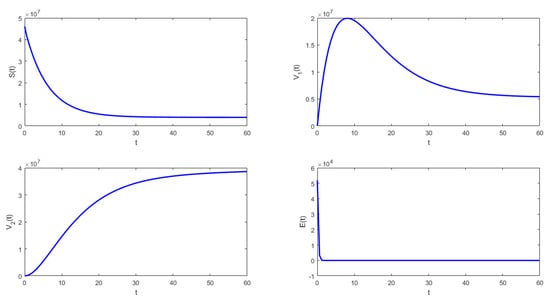
Figure 2. Numerical simulation of system (1) with the following values for the parameters: ${\beta }_I=1\times {10}^{-6}$, ${\beta }_A=1\times {10}^{-6}$, ${\nu }_1=0.15$, ${\nu }_2=0.1$, $\tau =0.1<{\tau }_1^{*}$, and ${\mathcal{R}}_0\approx 0.87<1$.

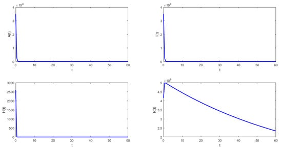
Figure 3. Numerical simulation of system (1) with the following values for the parameters: ${\beta }_I=1\times {10}^{-6}$, ${\beta }_A=1\times {10}^{-6}$, ${\nu }_1=0.15$, ${\nu }_2=0.1$, $\tau =0.1$, and ${\mathcal{R}}_0\approx 0.87<1$.

Figure 4 shows that under the conditions stated in Theorem 9, the solution of system (1) approaches the endemic equilibrium point. In this case, the latent $E\left(t\right)$, infected $I\left(t\right)$, and asymptomatic $A\left(t\right)$ subpopulations do not approach zero when $t\to \infty$. The susceptible $S\left(t\right)$, vaccinated with one dose $V_1\left(t\right)$, and vaccinated with two doses $V_2\left(t\right)$ subpopulations also approach values different than zero. This scenario is a public health concern since there are people permanently spreading SARS-CoV-2 despite the vaccination of some proportion of the susceptible population and the fact that the model assumes lifelong immunity.

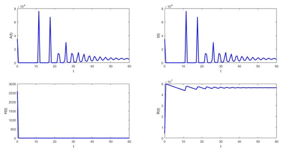
Figure 4. Numerical simulation of system (1) with the following values for the parameters: ${\beta }_I=0.16\times {10}^{-4}$, ${\beta }_A=0.16\times {10}^{-4}$, ${\nu }_1=0.15$, ${\nu }_2=0.1$, $\tau =0.1<{\tau }_1^{*}$, and ${\mathcal{R}}_0\approx 14>1$.

The following isthe last scenario that we consider when we obtain periodic solutions of system (1). Figure 5 and Figure 6 show that under the conditions stated in Theorem 9, the solution of system (1) undergoes a Hopf bifurcation where a periodic solution arises for a threshold time delay $\tau ={\tau }_1^{*}$. Figure 5 shows the susceptible $S\left(t\right)$, vaccinated with one dose $V_1\left(t\right)$, vaccinated with two doses $V_2\left(t\right)$, and latent $E\left(t\right)$ subpopulations. Note that these first three aforementioned subpopulations oscillate, as the theoretical results proved. However, notice that in order to obtain conditions such that periodic solutions arise, the time delay must satisfy Equation (45). This threshold time delay depends on parameters ${\nu }_1$ and d. One way to increase the time delay is by decreasing the proportion of first-vaccinated people, i.e., decreasing ${\nu }_1$. However, when the time delay is large there is no guarantee that the solutions of the delayed differential equation system are positive. In reality, the time delays are small since they represent the time it takes to obtain some immune protection from the vaccine. Thus, in the real world, the Hopf bifurcation scenario is unfeasible. We presented this unrealistic scenario with a large time delay in order to show that, mathematically, the system undergoes a Hopf bifurcation. Finally, Figure 5 shows the phase-space plot for three state variables ($S\left(t\right)$, $V_1\left(t\right)$, and $V_2\left(t\right)$), where the periodic behavior for these three subpopulations can be observed. These results are in good agreement with the theoretical results presented in the previous section.

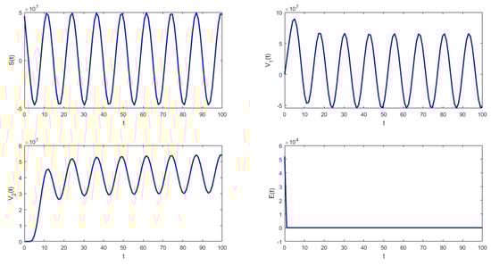
Figure 5. Numerical simulation of system (1) with the following values for the parameters: ${\beta }_I=0.02\times {10}^{-5}$, ${\beta }_A=0.02\times {10}^{-5}$, ${\nu }_1=1.5$, ${\nu }_2=2.1$, $\tau =3.1\approx {\tau }_1^{*}$, and ${\mathcal{R}}_0\approx 0.17<1$.

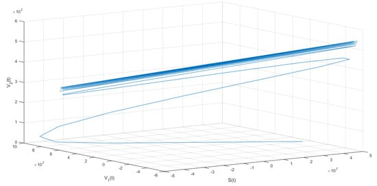
Figure 6. Numerical simulation of system (1) with the following values for the parameters: ${\beta }_I=0.02\times {10}^{-5}$, ${\beta }_A=0.02\times {10}^{-5}$, ${\nu }_1=1.5$, ${\nu }_2=2.1$, $\tau =3.1\approx {\tau }_1^{*}$, and ${\mathcal{R}}_0\approx 0.17<1$.

By analyzing the influence of various parameters in the simulations in the vaccination model, we can conclude that

• From Figure 2, it can be seen that when ${\mathcal{R}}_0<1$, that which is established in Theorem 7 is verified. In this case, the solutions tend to the equilibrium point $L^0$ defined in (14), and the behavior is stable. From a biological point of view, based on the chosen parameter values, if the susceptible population is subject to the vaccination process, growth is noted in the vaccinated subpopulations.
• In Figure 3, the validity of Theorem 9 is verified. In this case, the solutions tend to the equilibrium point $L^{*}$ and the behavior is stable.
• From Figure 4 and Figure 5, it can be seen that for the parameters established with ${\mathcal{R}}_0<1$, that which is established in Theorem 8 is verified.In this case, the solutions $S\left(t\right),V_1\left(t\right)$ and $V_2\left(t\right)$ are periodic when $\tau$ is around the threshold value ${\tau }_1^{*}$. Therefore, system (1) has a periodic solution branch that bifurcates from equilibrium $L^0$ near $\tau ={\tau }_1^{*}$.

6. Conclusions

Using mathematical tools, it is possible to obtain information about the dynamics of many infectious diseases. This mathematical approach also helps to assess the possible effects of health policies on the evolution of infectious disease processes. Mathematical models provide information that is often difficult to anticipate due to the complexity of the spread of viruses in a population.

In this work, we constructed a new COVID-19 mathematical model that includes individuals that have been vaccinated with different number of doses. The model developed is based on a system of delay differential equations and takes into account the time it takes for the vaccine to provide immune protection against SARS-CoV-2. This delay time is included in the system as a time-discrete delay in the equations of susceptible individuals and for people who have been vaccinated with one dose. First, we obtained the disease-free equilibrium point and studied the local stability analysis by computing the basic reproduction number ${\mathcal{R}}_0$. This crucial secondary parameter depends mainly on the transmission rate of SARS-CoV-2, the vaccine efficacy, and the vaccination rates for first and second dose. We found that if ${\mathcal{R}}_0<1$ and the time delays are less than some critical threshold ${\tau }^{*}$, then the disease-free equilibrium is locally stable. Thus, if public health authorities are able to reduce transmission rates and increase vaccination rates, the burden of the COVID-19 pandemic can be reduced. We also show that the model has a unique endemic equilibrium point when ${\mathcal{R}}_0>1$. We find a critical value ${\tau }^{*}$ where the disease-free equilibrium point loses stability and the time delay of the system induces the appearance of a Hopf bifurcation. Finally, with the appropriate choice of parameters, numerical simulations were presented to provide further corroboration of the theoretical results. From a real-world viewpoint, it is important to remark that periodic solutions arising from the Hopf bifurcation would not occur since the threshold value ${\tau }^{*}$ is much larger than potentially realistic values of the time delay for the vaccination against SARS-CoV-2. In addition, it is important to mention that in reality, the time delay is relatively small since it represents the time that it takes for the vaccine to start providing immunity against SARS-CoV-2. The numerical simulations of the considered scenarios here show positive solutions, but under different unrealistic conditions, such as large time delays, the solutions can be negative. In summary, we can conclude that the model provides a reasonable realistic scenario for the beginning of the COVID-19 pandemic when vaccines became available. However, similar to any mathematical model related to the full real-world situation, there are limitations. One important limitation of our model is the assumption that the vaccines as well as the natural infection provide lifelong immunity. The model for a short time period provides a good approximation regarding immunity since there is some period of full immunity. The proposed model can be adapted for other diseases where vaccine and natural infection provide lifelong immunity. Future work can be envisioned considering the loss of immunity. Additionally, different SARS-CoV-2 variants could be included as well as cross-immunity. This work could also be extended by including populations with booster doses against SARS-CoV-2. Furthermore, the inclusion of several time delays would entail a greater difficulty of solution of the mathematical model. In this article, we leave an open problem. We proved the positivity of the solution of the mathematical model when $\tau$ approaches zero, which still deals with a delayed system; however, finding an interval for the time delay such that the positivity can be guaranteed would be very interesting and challenging.

References

- Abila, D.B.; Dei-Tumi, S.D.; Humura, F.; Aja, G.N. We need to start thinking about promoting the demand, uptake, and equitable distribution of COVID-19 vaccines NOW! Public Health Pract. 2020, 1, 100063. [Google Scholar] [CrossRef]
- Moghadas, S.M.; Vilches, T.N.; Zhang, K.; Nourbakhsh, S.; Sah, P.; Fitzpatrick, M.C.; Galvani, A.P. Evaluation of COVID-19 vaccination strategies with a delayed second dose. PLoS Biol. 2021, 19, e3001211. [Google Scholar]
- Ao, D.; Lan, T.; He, X.; Liu, J.; Chen, L.; Baptista-Hon, D.T.; Zhang, K.; Wei, X. SARS-CoV-2 Omicron variant: Immune escape and vaccine development. MedComm 2022, 3, e126. [Google Scholar] [CrossRef] [PubMed]
- Bushman, M.; Kahn, R.; Taylor, B.P.; Lipsitch, M.; Hanage, W.P. Population impact of SARS-CoV-2 variants with enhanced transmissibility and/or partial immune escape. Cell 2021, 184, 6229–6242. [Google Scholar] [PubMed]
- Clemente-Suárez, V.J.; Hormeño-Holgado, A.; Jiménez, M.; Benitez-Agudelo, J.C.; Navarro-Jiménez, E.; Perez-Palencia, N.; Maestre-Serrano, R.; Laborde-Cárdenas, C.C.; Tornero-Aguilera, J.F. Dynamics of population immunity due to the herd effect in the COVID-19 pandemic. Vaccines 2020, 8, 236. [Google Scholar]
- Dyson, L.; Hill, E.M.; Moore, S.; Curran-Sebastian, J.; Tildesley, M.J.; Lythgoe, K.A.; House, T.; Pellis, L.; Keeling, M.J. Possible future waves of SARS-CoV-2 infection generated by variants of concern with a range of characteristics. Nat. Commun. 2021, 12, 5730. [Google Scholar] [CrossRef]
- Gonzalez-Parra, G.; Arenas, A.J. Nonlinear dynamics of the introduction of a new SARS-CoV-2 variant with different infectiousness. Mathematics 2021, 9, 1564. [Google Scholar] [CrossRef]
- Harvey, W.T.; Carabelli, A.M.; Jackson, B.; Gupta, R.K.; Thomson, E.C.; Harrison, E.M.; Ludden, C.; Reeve, R.; Rambaut, A.; Peacock, S.J.; et al. SARS-CoV-2 variants, spike mutations and immune escape. Nat. Rev. Microbiol. 2021, 19, 409–424. [Google Scholar] [CrossRef]
- Murray, J.D. Mathematical Biology I: An Introduction, Volume 17 of Interdisciplinary Applied Mathematics; Springer: New York, NY, USA, 2002. [Google Scholar]
- Keener, J.P. Biology in Time and Space: A Partial Differential Equation Modeling Approach; American Mathematical Society: Ann Arbor, MI, USA, 2021; Volume 50. [Google Scholar]
- Frassu, S.; Galván, R.R.; Viglialoro, G. Uniform in time L∞-estimates for an attraction-repulsion chemotaxis model with double saturation. Discret. Contin. Dyn. Syst.-B 2023, 28, 1886–1904. [Google Scholar]
- Grave, M.; Viguerie, A.; Barros, G.F.; Reali, A.; Coutinho, A.L. Assessing the spatio-temporal spread of COVID-19 via compartmental models with diffusion in Italy, USA, and Brazil. Arch. Comput. Methods Eng. 2021, 28, 4205–4223. [Google Scholar]
- Guglielmi, N.; Iacomini, E.; Viguerie, A. Delay differential equations for the spatially resolved simulation of epidemics with specific application to COVID-19. Math. Methods Appl. Sci. 2022, 45, 4752–4771. [Google Scholar] [CrossRef]
- Ayoub, H.H.; Chemaitelly, H.; Abu-Raddad, L.J. Epidemiological Impact of Novel Preventive and Therapeutic HSV-2 Vaccination in the United States: Mathematical Modeling Analyses. Vaccines 2020, 8, 366. [Google Scholar] [CrossRef] [PubMed]
- Benest, J.; Rhodes, S.; Quaife, M.; Evans, T.G.; White, R.G. Optimising Vaccine Dose in Inoculation against SARS-CoV-2, a Multi-Factor Optimisation Modelling Study to Maximise Vaccine Safety and Efficacy. Vaccines 2021, 9, 78. [Google Scholar] [CrossRef] [PubMed]
- Gozalpour, N.; Badfar, E.; Nikoofard, A. Transmission dynamics of novel coronavirus SARS-CoV-2 among healthcare workers, a case study in Iran. Nonlinear Dyn. 2021, 105, 3749–3761. [Google Scholar] [CrossRef] [PubMed]
- Martinez-Rodriguez, D.; Gonzalez-Parra, G.; Villanueva, R.J. Analysis of key factors of a SARS-CoV-2 vaccination program: A mathematical modeling approach. Epidemiologia 2021, 2, 140–161. [Google Scholar] [CrossRef]
- Yang, H.M.; Junior, L.P.L.; Castro, F.F.M.; Yang, A.C. Evaluating the impacts of relaxation and mutation in the SARS-CoV-2 on the COVID-19 epidemic based on a mathematical model: A case study of São Paulo State (Brazil). Comput. Appl. Math. 2021, 40, 272. [Google Scholar] [CrossRef]
- Babasola, O.; Kayode, O.; Peter, O.J.; Onwuegbuche, F.C.; Oguntolu, F.A. Time-delayed modelling of the COVID-19 dynamics with a convex incidence rate. Inform. Med. Unlocked 2022, 35, 101124. [Google Scholar] [CrossRef]
- Dell’Anna, L. Solvable delay model for epidemic spreading: The case of Covid-19 in Italy. Sci. Rep. 2020, 10, 15763. [Google Scholar] [CrossRef]
- Devipriya, R.; Dhamodharavadhani, S.; Selvi, S. SEIR model FOR COVID-19 Epidemic using DELAY differential equation. In Proceedings of the Journal of Physics: Conference Series, Nanchang, China, 26–28 October 2021; IOP Publishing: Bristol, UK, 2021; Volume 1767, p. 012005. [Google Scholar]
- Gonzalez-Parra, G. Analysis of delayed vaccination regimens: A mathematical modeling approach. Epidemiologia 2021, 2, 271–293. [Google Scholar] [CrossRef]
- Paul, S.; Lorin, E. Estimation of COVID-19 recovery and decease periods in Canada using delay model. Sci. Rep. 2021, 11, 23763. [Google Scholar] [CrossRef]
- Pell, B.; Johnston, M.D.; Nelson, P. A data-validated temporary immunity model of COVID-19 spread in Michigan. Math. Biosci. Eng. 2022, 19, 10122–10142. [Google Scholar] [CrossRef]
- Shayak, B.; Sharma, M.M.; Gaur, M.; Mishra, A.K. Impact of reproduction number on multiwave spreading dynamics of COVID-19 with temporary immunity: A mathematical model. Int. J. Infect. Dis. 2021, 104, 649–654. [Google Scholar] [CrossRef]
- Shayak, B.; Sharma, M.M.; Rand, R.H.; Singh, A.; Misra, A. A Delay differential equation model for the spread of COVID-19. Int. J. Eng. Res. Appl. 2020, 10, 1–13. [Google Scholar]
- Benlloch, J.M.; Cortés, J.C.; Martínez-Rodríguez, D.; Julián, R.S.; Villanueva, R.J. Effect of the early use of antivirals on the COVID-19 pandemic. A computational network modeling approach. Chaos Solitons Fractals 2020, 140, 110168. [Google Scholar] [CrossRef] [PubMed]
- Bhadauria, A.S.; Pathak, R.; Chaudhary, M. A SIQ mathematical model on COVID-19 investigating the lockdown effect. Infect. Dis. Model. 2021, 6, 244–257. [Google Scholar] [CrossRef]
- Dobrovolny, H.M. Modeling the role of asymptomatics in infection spread with application to SARS-CoV-2. PLoS ONE 2020, 15, e0236976. [Google Scholar] [CrossRef]
- Hamou, A.A.; Rasul, R.R.; Hammouch, Z.; Özdemir, N. Analysis and dynamics of a mathematical model to predict unreported cases of COVID-19 epidemic in Morocco. Comput. Appl. Math. 2022, 41, 289. [Google Scholar] [CrossRef]
- González-Parra, G.; Díaz-Rodríguez, M.; Arenas, A.J. Mathematical modeling to study the impact of immigration on the dynamics of the COVID-19 pandemic: A case study for Venezuela. Spat. Spatio-Temporal Epidemiol. 2022, 43, 100532. [Google Scholar] [CrossRef] [PubMed]
- Mahrouf, M.; Boukhouima, A.; Zine, H.; Lotfi, E.M.; Torres, D.F.; Yousfi, N. Modeling and forecasting of COVID-19 spreading by delayed stochastic differential equations. Axioms 2021, 10, 18. [Google Scholar] [CrossRef]
- Pham, H. On estimating the number of deaths related to Covid-19. Mathematics 2020, 8, 655. [Google Scholar] [CrossRef]
- Pinter, G.; Felde, I.; Mosavi, A.; Ghamisi, P.; Gloaguen, R. COVID-19 pandemic prediction for Hungary; a hybrid machine learning approach. Mathematics 2020, 8, 890. [Google Scholar] [CrossRef]
- Dobrovolny, H.M. Quantifying the effect of remdesivir in rhesus macaques infected with SARS-CoV-2. Virology 2020, 550, 61–69. [Google Scholar] [CrossRef]
- Fain, B.; Dobrovolny, H.M. Initial Inoculum and the Severity of COVID-19: A Mathematical Modeling Study of the Dose-Response of SARS-CoV-2 Infections. Epidemiologia 2020, 1, 5–15. [Google Scholar] [CrossRef]
- Ghosh, I. Within host dynamics of SARS-CoV-2 in humans: Modeling immune responses and antiviral treatments. SN Comput. Sci. 2021, 2, 482. [Google Scholar] [CrossRef] [PubMed]
- Dinleyici, E.C.; Borrow, R.; Safadi, M.A.P.; van Damme, P.; Munoz, F.M. Vaccines and routine immunization strategies during the COVID-19 pandemic. Hum. Vaccines Immunother. 2021, 17, 400–407. [Google Scholar] [CrossRef]
- Haque, A.; Pant, A.B. Efforts at COVID-19 Vaccine Development: Challenges and Successes. Vaccines 2020, 8, 739. [Google Scholar] [CrossRef] [PubMed]
- Hodgson, S.H.; Mansatta, K.; Mallett, G.; Harris, V.; Emary, K.R.; Pollard, A.J. What defines an efficacious COVID-19 vaccine? A review of the challenges assessing the clinical efficacy of vaccines against SARS-CoV-2. Lancet Infect. Dis. 2021, 21, e26–e35. [Google Scholar] [CrossRef]
- Van den Driessche, P.; Watmough, J. Further Notes on the Basic Reproduction Number; Springer: Berlin/Heidelberg, Germany, 2008; pp. 159–178. [Google Scholar]
- Hale, J.K. Theory of Functional Differential Equations, 2nd ed.; Applied Mathematical Sciences 3; Springer: Berlin/Heidelberg, Germany, 1977. [Google Scholar]
- Nelson, R. COVID-19 disrupts vaccine delivery. Lancet Infect. Dis. 2020, 20, 546. [Google Scholar] [CrossRef]
- Weintraub, R.L.; Subramanian, L.; Karlage, A.; Ahmad, I.; Rosenberg, J. COVID-19 Vaccine To Vaccination: Why Leaders Must Invest In Delivery Strategies Now: Analysis describe lessons learned from past pandemics and vaccine campaigns about the path to successful vaccine delivery for COVID-19. Health Aff. 2021, 40, 33–41. [Google Scholar] [CrossRef]
- Mahase, E. COVID-19: Pfizer vaccine efficacy was 52% after first dose and 95% after second dose, paper shows. BMJ 2020, 371, m4826. [Google Scholar] [CrossRef]
- Hasanoglu, I.; Korukluoglu, G.; Asilturk, D.; Cosgun, Y.; Kalem, A.K.; Altas, A.B.; Kayaaslan, B.; Eser, F.; Kuzucu, E.A.; Guner, R. Higher viral loads in asymptomatic COVID-19 patients might be the invisible part of the iceberg. Infection 2021, 49, 117–126. [Google Scholar] [CrossRef] [PubMed]
- Ferguson, N.; Laydon, D.; Nedjati Gilani, G.; Imai, N.; Ainslie, K.; Baguelin, M.; Bhatia, S.; Boonyasiri, A.; Cucunuba Perez, Z.; Cuomo-Dannenburg, G.; et al. Report 9: Impact of non-pharmaceutical interventions (NPIs) to reduce COVID19 mortality and healthcare demand. Imp. Coll. Lond. 2020, 10, 491–497. [Google Scholar]
- Kinoshita, R.; Anzai, A.; Jung, S.m.; Linton, N.M.; Miyama, T.; Kobayashi, T.; Hayashi, K.; Suzuki, A.; Yang, Y.; Akhmetzhanov, A.R.; et al. Containment, Contact Tracing and Asymptomatic Transmission of Novel Coronavirus Disease (COVID-19): A Modelling Study. J. Clin. Med. 2020, 9, 3125. [Google Scholar] [CrossRef] [PubMed]
- Chen, Y.; Wang, A.; Yi, B.; Ding, K.; Wang, H.; Wang, J.; Xu, G. The epidemiological characteristics of infection in close contacts of COVID-19 in Ningbo city. Chin. J. Epidemiol. 2020, 41, 668–672. [Google Scholar]
- Mc Evoy, D.; McAloon, C.G.; Collins, A.B.; Hunt, K.; Butler, F.; Byrne, A.W.; Casey, M.; Barber, A.; Griffin, J.M.; Lane, E.A.; et al. The relative infectiousness of asymptomatic SARS-CoV-2 infected persons compared with symptomatic individuals: A rapid scoping review. medRxiv 2020. [Google Scholar] [CrossRef]
- Zhao, H.J.; Lu, X.X.; Deng, Y.B.; Tang, Y.J.; Lu, J.C. COVID-19: Asymptomatic carrier transmission is an underestimated problem. Epidemiol. Infect. 2020, 148, 1–7. [Google Scholar] [CrossRef]
- Fred Brauer, J.A.N. The Qualitative Theory of Ordinary Differential Equations: An Introduction; Dover Publications: Garden City, NY, USA, 1989. [Google Scholar]
- Van den Driessche, P.; Watmough, J. Reproduction numbers and sub-threshold endemic equilibria for compartmental models of disease transmission. Math. Biosci. 2002, 180, 29–48. [Google Scholar] [CrossRef]
- Wang, X. A Simple Proof of Descartes’s Rule of Signs. Am. Math. Mon. 2004, 111, 525. [Google Scholar] [CrossRef]
- Karaaslanlı, C.Ç. Bifurcation Analysis and Its Applications; INTECH Open Access Publisher: London, UK, 2012. [Google Scholar]
- Krauskopf, B.; Sieber, J. Bifurcation analysis of systems with delays: Methods and their use in applications. In Controlling Delayed Dynamics; Springer: Berlin/Heidelberg, Germany, 2023; pp. 195–245. [Google Scholar]
- Bernard, S. Cell Population Dynamics—Lecture Notes; University Lyon Publishing: Lyon, France, 2021. [Google Scholar]
- Huang, Q.; Ma, Z. On stability of some transcendental equation. Ann. Diff. Eqs 1990, 6, 21–31. [Google Scholar]
- Shampine, L.F.; Thompson, S. Solving ddes in matlab. Appl. Numer. Math. 2001, 37, 441–458. [Google Scholar] [CrossRef]
- Shampine, L.F.; Thompson, S. Numerical solution of delay differential equations. In Delay Differential Equations; Springer: Berlin/Heidelberg, Germany, 2009; pp. 1–27. [Google Scholar]
- The World Bank. 2021. Available online: https://data.worldbank.org/ (accessed on 1 March 2022).
- Li, Q.; Guan, X.; Wu, P.; Wang, X.; Zhou, L.; Tong, Y.; Ren, R.; Leung, K.S.; Lau, E.H.; Wong, J.Y.; et al. Early transmission dynamics in Wuhan, China, of novel coronavirus–infected pneumonia. N. Engl. J. Med. 2020, 382, 1199–1207. [Google Scholar] [CrossRef] [PubMed]
- IHME COVID-19 Forecasting Team. Modeling COVID-19 scenarios for the United States. Nat. Med. 2021, 27, 94–105. [Google Scholar] [CrossRef] [PubMed]
- Lauer, S.A.; Grantz, K.H.; Bi, Q.; Jones, F.K.; Zheng, Q.; Meredith, H.R.; Azman, A.S.; Reich, N.G.; Lessler, J. The incubation period of coronavirus disease 2019 (COVID-19) from publicly reported confirmed cases: Estimation and application. Ann. Intern. Med. 2020, 172, 577–582. [Google Scholar] [CrossRef] [PubMed]
- Hoseinpour Dehkordi, A.; Alizadeh, M.; Derakhshan, P.; Babazadeh, P.; Jahandideh, A. Understanding epidemic data and statistics: A case study of COVID-19. J. Med Virol. 2020, 92, 868–882. [Google Scholar] [CrossRef] [PubMed]
- Quah, P.; Li, A.; Phua, J. Mortality rates of patients with COVID-19 in the intensive care unit: A systematic review of the emerging literature. Crit. Care 2020, 24, 1–4. [Google Scholar] [CrossRef]
- Paltiel, A.D.; Schwartz, J.L.; Zheng, A.; Walensky, R.P. Clinical outcomes of a COVID-19 vaccine: Implementation over efficacy: Study examines how definitions and thresholds of vaccine efficacy, coupled with different levels of implementation effectiveness and background epidemic severity, translate into outcomes. Health Aff. 2021, 40, 42–52. [Google Scholar]
- Centers for Disease Control and Prevention. 2020. Available online: https://www.cdc.gov/coronavirus/2019-nCoV/index.html (accessed on 1 March 2022).
- Oran, D.P.; Topol, E.J. Prevalence of Asymptomatic SARS-CoV-2 Infection: A Narrative Review. Ann. Intern. Med. 2020, 173, 362–367. [Google Scholar] [CrossRef]
Disclaimer/Publisher’s Note: The statements, opinions and data contained in all publications are solely those of the individual author(s) and contributor(s) and not of MDPI and/or the editor(s). MDPI and/or the editor(s) disclaim responsibility for any injury to people or property resulting from any ideas, methods, instructions or products referred to in the content. |
© 2023 by the authors. Licensee MDPI, Basel, Switzerland. This article is an open access article distributed under the terms and conditions of the Creative Commons Attribution (CC BY) license (https://creativecommons.org/licenses/by/4.0/).