Abstract
Solid oxide technology has gained importance due to its higher efficiencies compared to other current hydrogen technologies. The reversible mode allows working with both technologies (SOEC-SOFC), which makes it very attractive for mixed operations, both storage and generation, increasing its usage and therefore the viability of the technology implementation. To improve the performance of reversible stacks, developing adequate control strategies is of great importance. In order to design these strategies, suitable models are needed. These control-oriented models should be simple for an efficient controller design, but also they should include all phenomena that can be affected by the control law. This article introduces a control-oriented modeling of a reversible solid oxide stack (rSOS) for the implementation of control strategies considering thermal and degradation effects. The model is validated with experimental data of a 1.5 kW laboratory prototype, analyzing both polarization curves and dynamic responses to different current profiles and compositions. An error of less than 3% between the model and experimental responses has been obtained, demonstrating the validity of the proposed control-oriented model. The proposed model allows performing new and deeper analysis of the role of reversible solid oxide cells in 24/7 generation plants with renewable energy sources.
Keywords:
reversible solid oxide cells (rSOC); mathematical modeling; control-oriented modeling; thermal safety; hydrogen; stack degradation; experimental rSOC; solid oxide fuel cells; solid oxide electrolyzer MSC:
80-10
1. Introduction
The global need for decarbonization has led to a growing interest in the production and use of green hydrogen in an efficient, scalable and economical way. After a major role in the study of solid oxide cells at the beginning of the century, the reversible mode of operation has recently appeared as an alternative for combining power generation and chemical energy storage, increasing the possible usage times respect to only one mode of operation. Actually, two main types of solid oxide cell typologies, i.e., tubular and planar, are widely commercialized, but planar cells have attracted interest for stack construction due to their better performance instead of lower resistance [1]. The electrolyte of the reversible solid oxide stacks (rSOS) is commonly made of Yttria-stabilized zirconia (YSZ), and its operating temperature is about 700–900 °C [2]. More specifically, for electolyte-supported cells, the range of temperatures is 900–950 °C, and for electrode-supported cells, the range is 700–800 °C. Solid oxide technology has greater advantages than others, since due to the higher operation temperature, they consume less electricity thanks to the greater conversion efficiency led by the thermodynamical advantages. The energy needed for electrolysis decreases as the temperature increases; thus, SOECs (Solid Oxide Electrolyzers) can operate at a thermoneutral voltage in which the theoretical conversion efficiency of electricity to fuel is 100%. The operating temperature range is 700–950 °C. Up to now, rSOS is the only single system that can operate bi-directionally (electrolysis and power generation) and does not require the separation of power-to-gas (P2G) and gas-to-power (G2P) components [3].
Proper dynamics are important for model-based control. These control-oriented models should include the main phenomena affected by the control actions, but they should be sufficiently simple for an efficient controller design. Even though the modeling of rSOC can be completed designing multi-dimensional 2D and 3D models, this type of model requires an excessive computational load for control purposes. Instead, 1D or 0D (lumped) models are usually implemented [1]. Among the control-oriented models used for other hydrogen technologies, Pukrushpan et al. [4], Bao et al. [5] or Solsona et al. [6] presented their candidate models for proton exchange membrane (PEM) fuel cells. For solid oxide systems, different models have been developed [7,8], mainly considering fuel cell operation mode, while the works of reversible operation of SOC technology are more scarce. In addition, there is interest in the reversible operation for energy storage and usage routes for grid and demand balancing, and so the control-oriented models such as the one presented here become essential when designing reversible systems.
In the literature, there are different works that have tried to identify dynamics of reversible solid oxide cells but did not focus on control aspects. Motylinski et al. [9] presented an rSOC dynamic model to perform grid power balancing, focusing on the compatibility with wind profiles. The authors presented a cell model focused on the energy balance and its adaptation to a reduced electrical model. The model was scaled to a greater number of cells to satisfy the requirements of the electrical network. Liu et al. [10] studied strategies for the thermal safety analysis for the mode-switching process of a reversible solid oxide cell system. The authors used a simplified computational model of the rSOC system and a finite element method 1D model of the stack to determine the temperature distribution of the cell along the direction of the gas flow during the process. Frank et al. [11] introduced a model based on cascading one-sided stirred-tank reactors in order to obtain a 1D resolution in the flow direction. The models were designed to perform an analysis of the stack efficiency. Finally, orienting to embedded applications such as real-time simulations or online diagnostics, Ma et al. [12] proposed a multi-physical modeling of a 2D reversible tubular solid oxide cell. The authors introduced an iterative algorithm necessary to execute their non-linear model, avoiding possible solver stability issues.
An alternative approach is modeling the rSOC behavior as two separate systems (SOFC-SOEC). An example of this approach can be found in [13], where a two-stack model is used to analyze the energy balances and the oxygen purity. Unfortunately, the results were not validated experimentally. The same modeling technique was used by Hauck et al. [14] which used a model composed of two stacks with the aim of carrying out a thermodynamic analysis. The authors used empirical results found in the work of Kazempoor et al. [15] to check the simulations and find the influence of cell geometry and inlet gas composition in the thermodynamic behavior. Ni et al. [16] introduced a model focused on concentration losses to analyze their influence on the final response of reversible cells. Luo et al. [17] used a detailed model of a tubular cell to analyze the rSOC penetration and dynamic operation stability in a distributed system coupling wind generators, combustion engine and lithium-ion batteries. Finally, Botta et al. [18] introduced the importance of the thermal control strategies for rSOC. The study was carried out with decoupled models, which are both based in an SOFC template available in Modelica. The control strategies were validated through simulations. This work was one of the first studies dealing with the effects of controllers in rSOC.
Degradation is a crucial effect on stacks, since it determines the increase in power losses that the stack will experience throughout its useful life. Stack degradation is a vast field, ranging from materials analysis [19] to data science [20], with the goal of finding common behavior across different cells. The state of the art of degradation studies of reversible solid oxide systems has been recently presented by Yang et al. [21] and Khan et al. [22]. Among others, Zhang et al. [23] carried out a study on the degradation of solid oxide cells, concluding that the degradation is a more significant issue when operating in electrolysis mode. Knibbe et al. [24] studied the degradation of Ni-YSZ solid oxide electrolysis cells operated at high current densities, attributing the stack ohmic degradation to the increased polarization drop across the oxygen electrode. In a long-term analysis, Tietz et al. [25] performed a 9000-h study of an anode-supported solid oxide cell with a current density of 1 A/cm2 obtaining a certain degradation rate. Similarly, Blum et al. [26] obtained the degradation rates of two stacks with 20,000 and 50,000 h of operation. Focusing on modeling degradation effects, some studies such as [27,28,29] can be found, but the models are complex 2D or 3D models mainly focusing on the different types of degradation that are not suitable for control design purposes. The objective of this work will be to introduce the degradations in a simple and linear way, considering the long degradation studies found in the literature. For this purpose, the recent degradation works of Naeini et al. [30,31] have been taken as reference.
Finally, the modeling of rSOC including the dynamics of the agents to perform the balance of plant (BoP) as pumps, heat exchangers (HE), bypass valves, compressors, etc. are not widely studied in the rSOC literature. Some authors such as [11,32] explain the use of BoP agents, but they do not perform an explicit modeling; probably, they consider it unnecessary for their analysis, since the BoP is not always required for all the technology modeling analysis. However, in the present work, we consider it essential to study and understand the control strategies. Among those using solid oxide systems, Akikur et al. [33] performed simulations of rSOC systems in steady state presenting 0D BoP agents models, which include compressors and heat exchangers. Considering other approaches, Mottaghizadeh et al. [34] presented a BoP 0D model to carry out a feasibility study of building a system for energy storage based on rSOCs using hydrocarbon fuels. Going further, a model considering elements for the balance of plant of a PEM stack was introduced in [35]. However, this model only considers the agents necessarily for the fuel cell operation.
The purpose of this article is to develop a reliable control model of a reversible solid oxide stack prototype and present control aspects related to the regulation of voltage and temperature. The main contributions can be summarized as:
- Development of a practical control-oriented model for a reversible solid oxide stack prototype considering a linear degradation model.
- Validation of the proposed model with experimental data under different scenarios and the introduction of an offline algorithm to identify the unknown model parameters.
- Present the mathematical structure and the main considerations of the balance of plant agents and the controllers implemented for the optimal functioning of the system.
- Analyze the thermal effects of the controlled plant under different conditions.
In Section 2, an introduction of the laboratory stack description and the guidelines for developing the control-oriented model are presented. In Section 3, the balance of plant agents and its considerations are introduced. Section 4 describes the final model structure and proposed control strategy aimed to regulate the voltage and temperature of the stack. Then, the experiments, the model validation and the stack behavior analysis are given in Section 5. Finally, some conclusions are drawn in Section 7.
2. Mathematical Model
The prototype under study is shown in Figure 1, and a schematic illustration of the involved flows is shown in Figure 2. The anode-supported 30-cell stack with Ni-YSZ interconnections and the furnace are established as the main parts of the prototype. The balance of plant (BoP) agents are two heat exchangers (air–air and fuel–fuel), a boiler and a condenser. In Figure 2, the green tubes symbolize the inflows and its directions, whereas the red ones symbolize the outflows. Through a bypass valve, it is possible to introduce a certain amount of cooling air into the stack, while the necessary heat can be supplied through the oven to maintain the thermal balance of the plant.
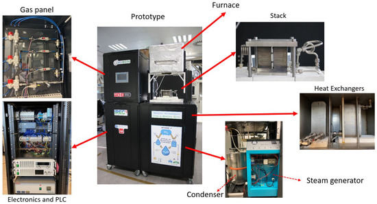
Figure 1.
Reversible solid oxide stack and the BoP agents implemented at IREC laboratory.
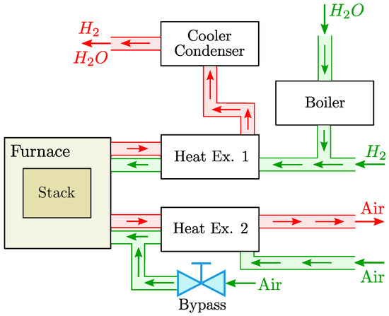
Figure 2.
A schematic illustration of the IREC solid oxide station operation including the balance of plant agents. The red channels denote the outlet flows, while the green channels denote the inlet ones.
The modeling of the system can be divided into three main submodels: the fluid dynamics (both in the manifolds and within the stack), the electrochemical (containing degradation) and the thermodynamic ones.
2.1. Fluid Dynamics: Manifolds Mass Flow
The dynamics of the manifolds is an important part of the model, determining both the inlet mass flow of the air channel, from the inlet manifold outlet mass flow, and the pressure inside the air channel, from the pressure of the outlet manifold, necessary to calculate the partial pressures of the gases. A manifold detailed analysis can be found in Pukrushpan et al. [4,35]. The manifold behavior is directly related to the mass conservation principle:
where m is the mass of the gas in the manifold volume and , are the input and output mass flow rates of the manifold, respectively. If the temperature is constant, the pressure manifold dynamics can be described by:
being the air gas constant, V the manifold volume and T the temperature.
The air inlet of the system is represented by the inlet manifold. From a certain inlet air flow, the inlet manifold will establish a certain air flow at its outlet, which will be the cathode air inlet, which is characterized by a resultant pressure and temperature. This outlet air flow can be linearized as a function of the inlet manifold valve constant as:
being the cathode pressure and the inlet manifold pressure given by:
being the inlet manifold volume and the air specific heat ratio. On the other hand, the dynamics of pressure of cathode outlet manifold is modeled in similar way:
where is the cathode mass flow, is the outlet manifold volume and the output air mass flow from the outlet manifold obtained from the relationship:
where is the outlet manifold constant and is the atmospheric pressure.
2.2. Fluid Dynamics: Stack Mass Flow
The mass flow model encompasses both the mass transport dynamics and the mass flow dynamics as well as the gas temperature ones, defining the partial pressures of each gas that will take place in the electrochemical model. The mass flow model will describe the dynamics of O2 and N2 in the air channel and those of H2O and H2 in the fuel channel, obtaining their respective partial pressures.
Assuming an ideal gas behavior, the partial pressures of the gas can be computed as:
where R is the universal gas constant. denotes the volumes of the anode () or the cathode (). The mass balance of each gas is computed as:
where , and are the inlet, reacted and outlet mass flows of the gas, respectively. Taking the number of cells (), the molar mass () and the Faraday constant (F), the reacted mass flow is given by
Notice that only H2O and O2 react. Finally, the input mass flow of each gas is computed as:
where and denote the mass fraction, being the ratio between the mass of each gas and the total mass of the mixture. The compositions of air and fuel will have a certain amount of each element. The mass fraction will be obtained from the molar fractions () used for the experiments. In the case of study, air is considered 21% of O2 and 79% of N2, while the fuel will be characterized by some percentages () of H2 and H2O. Finally, the output flows of the anode and cathode are calculated as:
being , experimental constants of the cathode and anode, respectively.
2.3. Electrochemical Model
The presented model describes the electrochemistry of the reaction and the polarization voltages. It is divided in four parts: Nernst voltage (), ohmic losses (), activation losses () and concentration losses (). The previous voltages define the operating voltage of the cell:
The signs of the previous equation can be modified depending on the operation mode. If operating in SOFC mode, the applied current is positive and the cell voltage is given by Equation (13), with . When operating in SOEC mode, the current is negative, and therefore:
Once the voltage of the cell is obtained, the voltage of the overall stack results:
being the number of cells.
2.3.1. Nernst Voltage
The Nernst equation describe the reversible cell voltage and its voltage variations as a function of gas compositions:
being , and the respective gas pressures, R the universal gas constant and the exponent representing the stoichiometric coefficient of the electrochemical reaction for oxygen. The term denotes the ideal or reversible voltage, which can be expressed as:
being the change in Gibbs free energy at standard temperature and pressure with pure reactants.
2.3.2. Ohmic Losses
Ohmic losses are difficult to model, as they depend on multiple phenomena. In particular, ohmic losses vary with the stack degradation. However, the resistive losses of the electrodes and the flow of the electrolyte ions are proportional to the current density, and usually, the area specific resistance (ASR), which denotes the resistance per cm2, can be used to model the ohmic voltage losses as:
being the current density in . Since ASR can be modeled, approximated, or identified, there is more than one way to define this parameter. However, working with stacks, the resistance that models the ohmic losses is the intrinsic resistance of each layer/material that constitutes the stack (electrolyte, electrodes, metal mesh between cells, metal inter-connectors, endplates) and the contact resistance between each layer:
Due to different orders of magnitude between the agents, the previous expression can be simplified to:
being the electrolyte thickness and the contact resistance. The variable corresponds to the electrolyte ionic conductivity which changes with temperature according to the Arrhenius equation:
where is the ionic conductivity pre-exponential factor and is the electrolyte activation energy [36].
2.3.3. Activation Losses
Activation losses occur at the electrode/electrolyte interface. They are caused by the steps of each electrochemical reaction, which has an associated activation energy, corresponding to the minimum energy required for a reaction to occur. The difference between activation energies and reaction rates govern the voltage losses in the electrode. The relation between the activation over-potential () and the current density is usually represented by the Butler–Volmer equation [37]:
The previous equation defines the kinetic losses associated with charge transfer reactions at each electrode–electrolyte interface. The parameter is the charge transfer coefficient and is related to the oxidation rate. The exchange current density () for the anode and cathode, respectively, can be determined based on [38] as:
being the total exchange current density .
Although some authors have presented that in low-density and high-density currents, the Butler–Volmer equation can be simplified to Tafel equations, these equations are only acceptable for a certain current range, since other quantities present too much error [39]. In the literature, the expression [40]:
is widely adopted and for this reason will be used in the proposed model.
2.3.4. Concentration Losses
Concentration losses are determined by changes in the concentration of the reactants at the electrode surfaces. Specifically, the reactions take place at certain locations on the electrode, which is called the Triple-Phase Boundary (TPB). TPB areas are the regions where the measured atmosphere, the metal catalyst and the electrolyte coexist [41]. The concentration losses can be expressed as a function of the partial pressures of the gases at the TPB as:
In order to obtain the cathode (ca) and anode (an) TPB partial pressures, Fick’s law can be applied, obtaining in the anode:
and in the cathode:
being , the thickness of the anode and cathode, the atmospheric pressure in bar, and the effective molecular diffusion coefficient of each gas. The previous coefficient considers molecular () and Knudsen () diffusion coefficients and is a function of the electrode porosity and tortuosity , and it can be expressed by the Bosanquet formula [42]:
The values of the effective molecular diffusion coefficients used for the studied stack are introduced in Table A1, Appendix A. A detailed description of these coefficients can be found on [39,43,44,45].
2.4. Thermodynamics
The stack temperature is essential for the electrochemical performance due to its influence on the partial pressures of the gases and on the kinetics of the charge transfer reactions. Therefore, in order to determine the amount of heat consumed or produced by the stack during operation, a thermal balance must be included. The heat produced or consumed Q will be determined by the difference between the total and the stack energies as:
being the electrical demand, the enthalpy reaction change and the thermal energy, where T can be computed as:
being the thermal mass of the stack and:
where denotes the stack heat, denotes the oven heat losses, denotes the gas convection losses and denotes the enviromental losses. For a single cell:
so therefore, for the stack formed by cells, and by taking as the hydrogen lowest heating value, the previous equation can be reformulated for the stack as:
The difference in temperature of the gases participating in the operation of the stack with an input or operation temperature different from that of the stack operation produces an alteration in the thermal balance through the introduction of convection losses. The convection heat of the gas, , is given by the Newton’s law of cooling,
being:
where is the stack temperature, is the temperature of the gas, is the specific heat of the gas and is its mass flow rate.
The non-adiabatic behavior of the stack oven walls supposes that part of the heat is lost to the environment, which can be modeled as a function of the temperature difference inside and outside the oven as:
being the surface of the oven, the heat transfer coefficient and the ambient temperature.
2.5. Stack Degradation: A Linear Approach
As the stack degradation is a much slower phenomenon than the ones involved in the control strategies, it is not necessary a highly detailed description in control-oriented models. Analyzing the existing literature focused on degradation from a mathematical modeling point of view, the works of Naeini et al. [30,31] can be taken as a reference. They developed a mathematical model of long-term degradation based on different databases of solid oxide cells degradation founded on the literature. The model aimed to predict long-term solid oxide cells performance under different operating conditions, including nickel coarsening and oxidation, anode pore size changes, degradation of anode and electrolyte conductivity, and sulfur poisoning. The previously mentioned effects can be included in a simplified function based on a degradation rate over time.
Therefore, the simplest way to express the evolution of stack degradation can be by the general expression:
where can be linear, exponential, etc. In this work for simplicity, it is considered that the degradation of the stack follows a linear relationship of degradation with respect to time as follows:
considering the cell degradation rate, describing the certain percentage of degradation that the stack will suffer after certain hours of operation. The union of Equations (19) and (42) defines the final expression used.
The degradation rate can be set according to the degradation experiments found in the literature. For example, in long-term analysis, Tietz et al. [25] performed a 9000 h study of an anode-supported solid oxide cell with a current density of 1 A/cm2 obtaining a voltage degradation rate of 3.8%/kh. Blum et al. presented in [26] a resume of degradation tests in two stacks operated continuously at 700 °C furnace temperature at a current density of 0.5 A/cm2 obtaining for 21,126 h a mean voltage degradation of 0.17%/kh in a smaller stack, while a larger stack presented with 50,691 h of operation and a voltage degradation of 0.8%/kh. In the durability study of a twenty-cell stack of Wonsyld et al. [46], low degradation rates of 1.44 m/cm2 per cycle in electrolysis and 0.10 m/cm2 per cycle in fuel cell mode were founded. A low degradation rate between 760 and 790 °C can also be concluded. Finally, Mai et al. [47], for a 1kW stack similar to the one studied here, obtained a degradation in terms of power of 1.6%/kh.
3. Balance of Plant Agents
The balance of plant (BoP) agents has been selected with the aim of optimizing the heat management, mainly by integrating two heat exchangers to pre-heat the inlet gases with the exhaust ones. BoP agents are important for the correct functioning of the stack and also for a high stack efficiency. The power considerations and modeling of the BoP for the laboratory rSOS shown in Figure 1 and Figure 2 are presented next.
3.1. Heat Exchangers
One of the most widely used methods to model heat exchangers (HE) is the method [48]. This method describes the relationship between the number of heat transfer units (NTU) and the effectiveness () of the heat exchanger for different flow modes, which has the form [33]:
being and the hot and cold fluid temperatures, respectively. Following the scheme in Figure 2, the fuel–fuel heat exchanger is block indicated as Heat Ex. 1, whereas the air–air heat exchanger is indicated as Heat Ex. 2. Note that the fuel HE receives the H2O from the boiler at water evaporation temperature and the rest of the gases, H2 and N2 (if contains), at ambient temperature. The resultant heating power can be formulated as:
being the heat capacity rate.
3.2. Boiler
The main function of the boiler is to convert water into steam. Once the vapor has reached the gaseous state, it is added to the hydrogen, and the composition is fed to the anode. For a certain water mass flow entering the boiler, the necessary boiler heating power to achieve the set-point temperature can be defined as:
where denotes the specific heat of the liquid and steam states, and is the initial temperature. and are the enthalpy and temperature of vaporization at standard pressure, respectively.
3.3. Condenser
The condenser is usually placed at the output of the stack receiving the output mass flow of H2 and H2O. Depending on the mode of operation, the output composition will have a certain percentage of each component. The main function of the condenser is to condense and accumulate the output H2O before the hydrogen is sent to the atmosphere through the extractor, ensuring a correct expulsion of the gases. Similar to the heat exchangers, the condenser can be also modeled by the method [48].
4. Control-Oriented Model and Control Definition
The differential equations given in Section 2 and Section 3 can be gathered in order to obtain a non-linear state-space model as:
where the set of control inputs are:
being the current density and and the control set-points of the oven and the bypass valve, respectively. The signal y corresponds to the vector of system output given by:
being the output mass flow of the air channel, the input mass flow of the outlet manifold and , the stack voltage and temperature. Finally, x is the vector of states given by:
corresponding to the masses of H2, H2O, N2, O2, the inlet and outlet manifolds pressures and the stack temperature, respectively.
Controllers for Thermal Safety
To achieve good performance and avoid potential damage and degradation, the stack temperature must be kept within a certain security limits. However, the solution does not go through an increase in flow rates to avoid undesired low or high temperatures, since it would mean an efficiency reduction. For this reason, control strategies for regulating the stack temperature and maintaining the efficiency are important.
The heating control of the furnace will be mainly important in the SOEC mode due to the endothermicity of the process when operated below the thermoneutral voltage. The controller is defined as:
where , , and are the reference and stack temperatures and the proportional and integral constants, respectively. The cooling controller actuates an air bypass valve to regulate the amount of cold air supplied. Contrary to oven control, the refrigeration control will be mainly important in the SOFC mode due to the exothermicity of the process. The controller is of the form:
Note that there must exist a coordination between controllers in order to not affect each other, producing unnecessary power losses.
5. Results and Analysis
In this section, we presented the parameter estimation of the proposed model for the laboratory testing prototype shown in Figure 1 and the corresponding experimental validation. The signals and readings of the sensors are processed in an external PC. A power source is programmed for the operation in SOEC mode, whereas for the operation in SOFC mode, an electronic load is used. The operating modes designed under security protocols are set using PLCs.
5.1. Parameter Estimation
The model proposed in Section 2 and Section 3 contains two sets of parameters. The first set includes parameters that can be measured or theoretically determined according to the system dimensions and components. This set of parameters is listed in Table A1 along with the values corresponding to the prototype implemented at IREC Laboratory. The second set of parameters cannot be theoretically determined or measured, and they need to be found by estimation from the experimental data. This set of parameters is gathered in the following vector:
and they are listed in Table A2. These parameters were estimated by solving the following numerical optimization problem:
where ) is the simulation response obtained from the proposed model and is the experimental response obtained from the prototype. As this is a non-linear optimization problem, the parameter range was limited by and . Different tests were performed to ensure that the responses did not correspond to local minima. The final obtained error corresponds to the difference between the voltage obtained and the experimental one, which is what minimizes the norm, corresponding to 3%. In the following sections, the model parameters have been identified using the algorithm described in this section and listed in Table A2.
5.2. Polarization Curves
Polarization curves are common stack characterization graphs, showing the relationship between cell voltage and current (iV curves). In order to validate the model through different experiments, the polarization curves of the electrolyzer mode operation, the fuel cell operation and the reversible mode operation will be performed under different conditions.
For the SOEC mode, a constant inlet flow rate of H2 was set. The fuel was characterized by 70% of H2O and 30% of H2. Figure 3a compares the experimental and model results. It can be observed that results predicted by the proposed model were quite close to the experimental values.
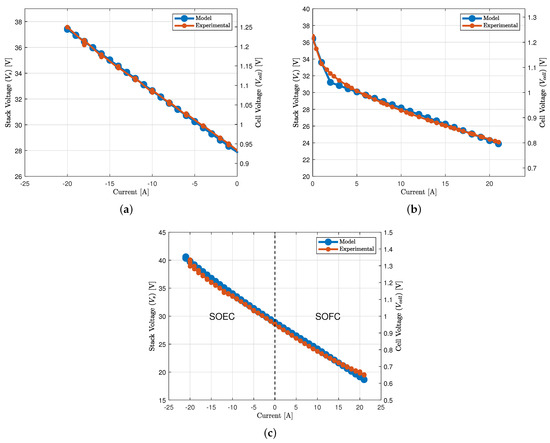
Figure 3.
Polarization curves. (a) Electrolysis mode polarization curve keeping a constant fuel composition with a ratio of 70% of H2O and 30% of H2. (b) Fuel cell mode polarization curve keeping a constant fuel composition with a ratio of 100% of H2. (c) Reversible mode polarization curve keeping a constant fuel composition with a ratio of 50% of H2O and 50% of H2.
For the SOFC mode, the fuel was characterized by 100% of H2, and a constant air flow rate of 37.5 L/min was set. The comparison between the simulation and experimental results is shown in Figure 3b. As in the SOEC case, the model provided a satisfactory estimation.
Once the SOFC and SOEC polarization curves were made, the last experiment performed was the reversible operation. For this experiment, the fuel composition was kept constant with a ratio of 50% of H2O and 50% of H2. Figure 3c shows the polarization curve under those conditions, where a smooth transition from SOEC (first applied mode) to SOFC can be observed. In fact, the controller automatically switches between load and power supply to perform this reversible operation. The iV curves are similar at all times, even at the time of switching from SOEC to SOFC mode.
5.3. Dynamic Response
In order to observe the dynamic response of the system, a profile operating first in SOEC mode and later in SOFC mode was chosen. The experiments had a duration of 4.2 h (≈15,000 s), which is a longer time compared to that necessary for the polarization curves. In SOEC mode, the input fuel composition used was 90% H2O and 10% H2, while for SOFC operation, the composition was 100% H2. Figure 4a compares the experimental and the model results. The orange lines show the experimental response to the introduced profile, while the discontinuous green lines show the response of the model presented to the same current profile. The model response is cleaner than the experimental results. Except at the moment of reversibility, around 2 h (7200s), where there is a change in the composition in OCV to go from SOEC to SOFC mode and the error is higher, the response is practically the same, with a total error of 3%. This error has been obtained after performing the minimization presented in Section 5.1. A total amount of 1.5 m3 of H2 was produced during the SOEC phase of the profile, while 0.9 m3 of H2 was consumed in the fuel cell mode. Figure 4b presents a comparison of the temperatures in the furnace. The model response shows the sensitivity of the model but also the effectiveness of the controllers, introducing a fairly fast correction response. The magnitude of the temperature variations is not remarkable, since the maximum deviation between the experimental and the simulated is ≈0.09% for the SOEC mode and ≈0.07% for the SOFC mode. Notice that the sensitivity of the temperature sensor is not high enough to detect less than 1 °C of variation.
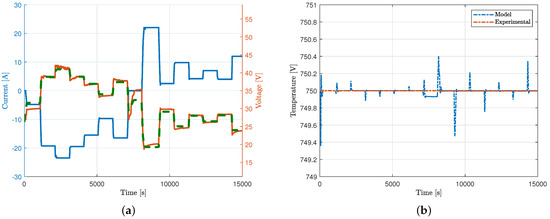
Figure 4.
Dynamic response. (a) Superposition of model (green) and experimental (orange) responses. Current in blue, the experimental voltage in orange and the model response in green. (b) Stack furnace temperature comparison.
5.4. Thermal Effects Analysis
Once the model is validated, a more detailed analysis of the thermal effects under the action of the controllers with different temperatures can be carried out. Figure 5a shows the influence of temperature on the system. The lines show the evolution of the voltage with a constant composition ratio of 50% of H2O and 50% of H2 and fixed mass flow rates (10 L/min) at different temperatures, between 650 and 950 °C. Analyzing the results in Figure 5a, the impact of temperature on the stack voltage, and therefore also on the power, can affect its performance. It can be noted that thermal effects are more marked during electrolysis than during fuel cell operation. In addition, it can be seen that lower voltages, and therefore higher yields, are obtained with higher temperatures.
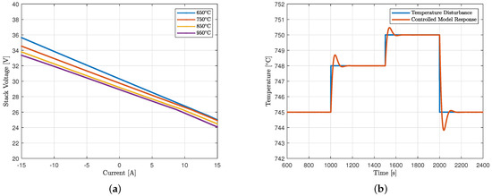
Figure 5.
Thermal analysis. (a) Temperature effects on the controlled reversible stack. (b) Temperature disturbances on the controlled reversible stack.
The capability of the temperature control for tracking set-point changes is analyzed in Figure 5b. To carry out this analysis, a constant current is maintained in electrolysis mode (where the greatest effect of temperature has been seen in Figure 5a) of −0.15 A/cm2, and disturbances with a range of 5 °C are introduced. It can be seen that the controllers are able to rapidly adjust the temperature to the new set-points. This is completed by injecting heat through the oven (t = 1000 s and t = 1500 s) when the set-points increase and also by switching off the heating and increasing the air-flow for cooling injected through the bypass valve when the set-point decrease (t = 2000 s).
6. Discussion
Although studies on reversible oxide cells have increased in recent years, the subject continues to have many parts of study to analyze, from materials, designs, efficiencies or controls. For the realization of model-based controls, control-oriented models containing the main dynamics of the system but fast enough to implement control strategies in real time are important. In the reversible mode, these models are not very abundant, since many of the existing dynamic models are multi-dimensional with a higher degree of complexity. In addition, some of the existing models or controls have not been verified experimentally. In this article, a mathematical modeling of a real stack of 30 cells has been presented, comparing the experimental and simulation responses. In addition, the necessary thermal control strategies are presented to maintain an efficient energy balance during long operations of this type of technology. Therefore, this article allows to present a control-oriented model of a real laboratory stack for possible studies of this type of technology in long-term operation.
7. Conclusions
Reversible solid oxide stacks have emerged as an important research topic due to the benefits and potential of this type of technology for the hydrogen-based energy transition. However, experimentally validated control-oriented models are not widely available so far. This article has introduced a complete model of a 30-cell stack, including the necessary BoP agents and controllers to ensure a proper operation. A linear degradation model is included in order to evaluate future long-term analysis. Four independent tests were carried out in order to characterize the reversible stack prototype. The predefined model parameters of the stack were introduced, while the unknown were estimated through a parameter identification algorithm. The mismatch between the experimental and model results has been around 3%, demonstrating the validity of the proposed model. This article has shown that some of the main challenges for the roll-out of the hydrogen technologies and their integration with renewable energy sources can be predicted and elucidated quickly and reliably by the proposed model.
Author Contributions
Conceptualization, H.d.P.G., M.T. and L.B.; methodology, H.d.P.G., M.T. and L.B.; software, H.d.P.G. and F.D.B.; validation, H.d.P.G., M.T., L.B. and F.D.B.; formal analysis, H.d.P.G., M.T. and L.B.; investigation, H.d.P.G. and F.D.B.; resources, H.d.P.G., M.T. and L.B.; data curation, M.T. and L.B.; writing—original draft preparation, H.d.P.G.; writing—review and editing, M.T., L.B., F.D.B., L.T. and J.L.D.-G.; visualization, H.d.P.G. and F.D.B.; supervision, L.T. and J.L.D.-G.; project administration, L.T., J.L.D.-G. and A.T.; funding acquisition, L.T., J.L.D.-G. and A.T. All authors have read and agreed to the published version of the manuscript.
Funding
The research leading to these results has received financial support from the Research and Universities Department of Catalonia Government under FI2022 program with grant agreement 2022-FI_B-00930 and from the Hy-FV project with grant agreement n°ACE014/20/000048.
Institutional Review Board Statement
Not applicable.
Informed Consent Statement
Not applicable.
Data Availability Statement
Not applicable.
Conflicts of Interest
The authors declare no conflict of interest.
Appendix A

Table A1.
Defined Parameters.
Table A1.
Defined Parameters.
| Estimated Parameter | Symbol | Value | Units |
|---|---|---|---|
| Stack Area | 63 | cm2 | |
| Stack Mass | 5.5 | kg | |
| Faraday Constant | F | 96,487 | C/mol |
| Number of Cells | 30 | - | |
| Oven Power | 2.75 | kW | |
| Oven Losses Constant | 0.7 | ||
| Universal Gas Constant | R | ||
| Air Gas Constant | |||
| H2 Molar Mass | g/mol | ||
| H2O Molar Mass | g/mol | ||
| O2 Molar Mass | g/mol | ||
| N2 Molar Mass | g/mol | ||
| Inlet Manifold Valve Constant | |||
| Outlet Manifold Valve Constant | |||
| Anode Valve Constant | |||
| Cathode Valve Constant | |||
| Electrolyte Thickness (8YSZ) | 10 | ||
| O2 Effective Diffusion Coefficient | |||
| H2O Effective Diffusion Coefficient | |||
| H2 Effective Diffusion Coefficient | |||
| Hydrogen Lowest Heating Value | 246,870 | ||
| Ionic Conductivity Pre-exponential Factor | 466 | s | |
| Electrolyte Activation Energy | J/mol |
Table A2.
Estimated Parameters.
Table A2.
Estimated Parameters.
| Estimated Parameter | Symbol | Value | Units |
|---|---|---|---|
| Cathode Phenomenological Coefficient | |||
| Anode Phenomenological Coefficient | |||
| Cathode Activation Energy | J/mol | ||
| Anode Activation Energy | J/mol | ||
| Contact Resistance | 0.3 |
References
- Marra, D.; Pianese, C.; Polverino, P.; Sorrentino, M. Models for Solid Oxide Fuel Cell Systems: Exploitation of Models Hierarchy for Industrial Design of Control and Diagnosis Strategies; Springer: Berlin/Heidelberg, Germany, 2016. [Google Scholar]
- Gómez, S.Y.; Hotza, D. Current developments in reversible solid oxide fuel cells. Renew. Sustain. Energy Rev. 2016, 61, 155–174. [Google Scholar] [CrossRef]
- Subotić, V.; Thaller, T.; Königshofer, B.; Menzler, N.H.; Bucher, E.; Egger, A.; Hochenauer, C. Performance assessment of industrial-sized solid oxide cells operated in a reversible mode: Detailed numerical and experimental study. Int. J. Hydrog. Energy 2020, 45, 29166–29185. [Google Scholar] [CrossRef]
- Pukrushpan, J.T.; Peng, H.; Stefanopoulou, A.G. Control-oriented modeling and analysis for automotive fuel cell systems. J. Dyn. Sys. Meas. Control 2004, 126, 14–25. [Google Scholar] [CrossRef]
- Bao, C.; Ouyang, M.; Yi, B. Modeling and control of air stream and hydrogen flow with recirculation in a PEM fuel cell system—I. Control-oriented modeling. Int. J. Hydrog. Energy 2006, 31, 1879–1896. [Google Scholar] [CrossRef]
- Solsona, M.; Kunusch, C.; Ocampo-Martinez, C. Control-oriented model of a membrane humidifier for fuel cell applications. Energy Convers. Manag. 2017, 137, 121–129. [Google Scholar] [CrossRef]
- Zhang, X.; Li, J.; Li, G.; Feng, Z. Development of a control-oriented model for the solid oxide fuel cell. J. Power Sources 2006, 160, 258–267. [Google Scholar] [CrossRef]
- Xing, Y.; Costa-Castello, R.; Na, J.; Renaudineau, H. Control-oriented modelling and analysis of a solid oxide fuel cell system. Int. J. Hydrog. Energy 2020, 45, 20659–20672. [Google Scholar] [CrossRef]
- Motylinski, K.; Kupecki, J.; Numan, B.; Hajimolana, Y.S.; Venkataraman, V. Dynamic modelling of reversible solid oxide cells for grid stabilization applications. Energy Convers. Manag. 2021, 228, 113674. [Google Scholar] [CrossRef]
- Liu, G.; Zhao, W.; Li, Z.; Xia, Z.; Jiang, C.; Kupecki, J.; Pang, S.; Deng, Z.; Li, X. Modeling and control-oriented thermal safety analysis for mode switching process of reversible solid oxide cell system. Energy Convers. Manag. 2022, 255, 115318. [Google Scholar] [CrossRef]
- Frank, M.; Deja, R.; Peters, R.; Blum, L.; Stolten, D. Bypassing renewable variability with a reversible solid oxide cell plant. Appl. Energy 2018, 217, 101–112. [Google Scholar] [CrossRef]
- Ma, R.; Gao, F.; Breaz, E.; Huangfu, Y.; Briois, P. Multidimensional reversible solid oxide fuel cell modeling for embedded applications. IEEE Trans. Energy Convers. 2017, 33, 692–701. [Google Scholar] [CrossRef]
- Iora, P.; Chiesa, P. High efficiency process for the production of pure oxygen based on solid oxide fuel cell–solid oxide electrolyzer technology. J. Power Sources 2009, 190, 408–416. [Google Scholar] [CrossRef]
- Hauck, M.; Herrmann, S.; Spliethoff, H. Simulation of a reversible SOFC with Aspen Plus. Int. J. Hydrog. Energy 2017, 42, 10329–10340. [Google Scholar] [CrossRef]
- Kazempoor, P.; Braun, R. Model validation and performance analysis of regenerative solid oxide cells for energy storage applications: Reversible operation. Int. J. Hydrog. Energy 2014, 39, 5955–5971. [Google Scholar] [CrossRef]
- Ni, M.; Leung, M.K.; Leung, D.Y. A modeling study on concentration overpotentials of a reversible solid oxide fuel cell. J. Power Sources 2006, 163, 460–466. [Google Scholar] [CrossRef]
- Luo, Y.; Shi, Y.; Zheng, Y.; Cai, N. Reversible solid oxide fuel cell for natural gas/renewable hybrid power generation systems. J. Power Sources 2017, 340, 60–70. [Google Scholar] [CrossRef]
- Botta, G.; Romeo, M.; Fernandes, A.; Trabucchi, S.; Aravind, P. Dynamic modeling of reversible solid oxide cell stack and control strategy development. Energy Convers. Manag. 2019, 185, 636–653. [Google Scholar] [CrossRef]
- Zhu, J.; Lin, Z. Degradations of the electrochemical performance of solid oxide fuel cell induced by material microstructure evolutions. Appl. Energy 2018, 231, 22–28. [Google Scholar] [CrossRef]
- Naeini, M.; Cotton, J.S.; Adams II, T.A. Data-Driven Modeling of Long-Term Performance Degradation in Solid Oxide Electrolyzer Cell System. In Computer Aided Chemical Engineering; Elsevier: Amsterdam, The Netherlands, 2022; Volume 49, pp. 847–852. [Google Scholar]
- Yang, C.; Guo, R.; Jing, X.; Li, P.; Yuan, J.; Wu, Y. Degradation mechanism and modeling study on reversible solid oxide cell in dual-mode—A review. Int. J. Hydrog. Energy 2022, 47, 37895–37928. [Google Scholar] [CrossRef]
- Khan, M.; Xu, X.; Knibbe, R.; Zhu, Z. Air electrodes and related degradation mechanisms in solid oxide electrolysis and reversible solid oxide cells. Renew. Sustain. Energy Rev. 2021, 143, 110918. [Google Scholar] [CrossRef]
- Zhang, X.; O’Brien, J.E.; O’Brien, R.C.; Housley, G.K. Durability evaluation of reversible solid oxide cells. J. Power Sources 2013, 242, 566–574. [Google Scholar] [CrossRef]
- Knibbe, R.; Traulsen, M.L.; Hauch, A.; Ebbesen, S.D.; Mogensen, M. Solid oxide electrolysis cells: Degradation at high current densities. J. Electrochem. Soc. 2010, 157, B1209. [Google Scholar] [CrossRef]
- Tietz, F.; Sebold, D.; Brisse, A.; Schefold, J. Degradation phenomena in a solid oxide electrolysis cell after 9000 h of operation. J. Power Sources 2013, 223, 129–135. [Google Scholar] [CrossRef]
- Blum, L.; Batfalsky, P.; De Haart, L.; Malzbender, J.; Menzler, N.H.; Peters, R.; Quadakkers, W.J.; Remmel, J.; Tietz, F.; Stolten, D. Overview on the Jülich SOFC development status. ECS Trans. 2013, 57, 23. [Google Scholar] [CrossRef]
- Gazzarri, J.; Kesler, O. Short-stack modeling of degradation in solid oxide fuel cells: Part I. Contact degradation. J. Power Sources 2008, 176, 138–154. [Google Scholar] [CrossRef]
- Navasa, M.; Graves, C.; Chatzichristodoulou, C.; Skafte, T.L.; Sundén, B.; Frandsen, H.L. A three dimensional multiphysics model of a solid oxide electrochemical cell: A tool for understanding degradation. Int. J. Hydrog. Energy 2018, 43, 11913–11931. [Google Scholar] [CrossRef]
- Rizvandi, O.B.; Miao, X.Y.; Frandsen, H.L. Multiscale modeling of degradation of full solid oxide fuel cell stacks. Int. J. Hydrog. Energy 2021, 46, 27709–27730. [Google Scholar] [CrossRef]
- Naeini, M.; Lai, H.; Cotton, J.S.; Adams, T.A. A Mathematical Model for Prediction of Long-Term Degradation Effects in Solid Oxide Fuel Cells. Ind. Eng. Chem. Res. 2021, 60, 1326–1340. [Google Scholar] [CrossRef]
- Naeini, M.; Cotton, J.S.; Adams, T.A. An eco-technoeconomic analysis of hydrogen production using solid oxide electrolysis cells that accounts for long-term degradation. Front. Energy Res. 2022, 10, 1015465. [Google Scholar] [CrossRef]
- Saarinen, V.; Pennanen, J.; Kotisaari, M.; Thomann, O.; Himanen, O.; Iorio, S.D.; Hanoux, P.; Aicart, J.; Couturier, K.; Sun, X.; et al. Design, manufacturing, and operation of movable 2× 10 kW size rSOC system. Fuel Cells 2021, 21, 477–487. [Google Scholar] [CrossRef]
- Akikur, R.; Saidur, R.; Ping, H.; Ullah, K. Performance analysis of a co-generation system using solar energy and SOFC technology. Energy Convers. Manag. 2014, 79, 415–430. [Google Scholar] [CrossRef]
- Mottaghizadeh, P.; Santhanam, S.; Heddrich, M.P.; Friedrich, K.A.; Rinaldi, F. Process modeling of a reversible solid oxide cell (r-SOC) energy storage system utilizing commercially available SOC reactor. Energy Convers. Manag. 2017, 142, 477–493. [Google Scholar] [CrossRef]
- Pukrushpan, J.T.; Stefanopoulou, A.G.; Peng, H. Control of Fuel Cell Power Systems: Principles, Modeling, Analysis and Feedback Design; Springer Science & Business Media: Berlin/Heidelberg, Germany, 2004. [Google Scholar]
- Weber, A.; Ivers-Tiffée, E. Materials and concepts for solid oxide fuel cells (SOFCs) in stationary and mobile applications. J. Power Sources 2004, 127, 273–283. [Google Scholar] [CrossRef]
- Noren, D.; Hoffman, M.A. Clarifying the Butler–Volmer equation and related approximations for calculating activation losses in solid oxide fuel cell models. J. Power Sources 2005, 152, 175–181. [Google Scholar] [CrossRef]
- Costamagna, P.; Honegger, K. Modeling of solid oxide heat exchanger integrated stacks and simulation at high fuel utilization. J. Electrochem. Soc. 1998, 145, 3995. [Google Scholar] [CrossRef]
- Chan, S.; Khor, K.; Xia, Z. A complete polarization model of a solid oxide fuel cell and its sensitivity to the change of cell component thickness. J. Power Sources 2001, 93, 130–140. [Google Scholar] [CrossRef]
- Wendel, C.H.; Gao, Z.; Barnett, S.A.; Braun, R.J. Modeling and experimental performance of an intermediate temperature reversible solid oxide cell for high-efficiency, distributed-scale electrical energy storage. J. Power Sources 2015, 283, 329–342. [Google Scholar] [CrossRef]
- Fukunaga, H.; Ihara, M.; Sakaki, K.; Yamada, K. The relationship between overpotential and the three phase boundary length. Solid State Ionics 1996, 86, 1179–1185. [Google Scholar] [CrossRef]
- Li, G.; Xiao, G.; Guan, C.; Hong, C.; Yuan, B.; Li, T.; Wang, J.Q. Assessment of thermodynamic performance of a 20 kW high-temperature electrolysis system using advanced exergy analysis. Fuel Cells 2021, 21, 550–565. [Google Scholar] [CrossRef]
- Hernández-Pacheco, E.; Singh, D.; Hutton, P.N.; Patel, N.; Mann, M.D. A macro-level model for determining the performance characteristics of solid oxide fuel cells. J. Power Sources 2004, 138, 174–186. [Google Scholar] [CrossRef]
- Bird, R.B. Transport phenomena. Appl. Mech. Rev. 2002, 55, R1–R4. [Google Scholar] [CrossRef]
- Bernadet, L.; Gousseau, G.; Chatroux, A.; Laurencin, J.; Mauvy, F.; Reytier, M. Influence of pressure on solid oxide electrolysis cells investigated by experimental and modeling approach. Int. J. Hydrog. Energy 2015, 40, 12918–12928. [Google Scholar] [CrossRef]
- Wonsyld, K.; Bech, L.; Nielsen, J.U.; Pedersen, C.F. Operational robustness studies of solid oxide electrolysis stacks. J. Energy Power Eng. 2015, 9, 128–140. [Google Scholar] [CrossRef]
- Mai, A.; Iwanschitz, B.; Schuler, J.A.; Denzler, R.; Nerlich, V.; Schuler, A. Hexis’ SOFC System Galileo 1000 N–Lab and Field Test Experiences. ECS Trans. 2013, 57, 73. [Google Scholar] [CrossRef]
- Yin, J.; Jensen, M.K. Analytic model for transient heat exchanger response. Int. J. Heat Mass Transf. 2003, 46, 3255–3264. [Google Scholar] [CrossRef]


Disclaimer/Publisher’s Note: The statements, opinions and data contained in all publications are solely those of the individual author(s) and contributor(s) and not of MDPI and/or the editor(s). MDPI and/or the editor(s) disclaim responsibility for any injury to people or property resulting from any ideas, methods, instructions or products referred to in the content. |
© 2023 by the authors. Licensee MDPI, Basel, Switzerland. This article is an open access article distributed under the terms and conditions of the Creative Commons Attribution (CC BY) license (https://creativecommons.org/licenses/by/4.0/).