Generalized Pandemic Model with COVID-19 for Early-Stage Infection Forecasting

Abstract

In this paper, we tackle the problem of forecasting future pandemics by training models with a COVID-19 time series. We tested this approach by producing one model and using it to forecast a non-trained time series; however, we limited this paper to the eight states with the highest population density in Mexico. We propose a generalized pandemic forecasting framework that transforms the time series into a dataset via three different transformations using random forest and backward transformations. Additionally, we tested the impact of the horizon and dataset window sizes for the training phase. A Wilcoxon test showed that the best transformation technique statistically outperformed the other two transformations with 100% certainty. The best transformation included the accumulated efforts of the other two plus a normalization that helped rescale the non-trained time series, improving the sMAPE from the value of 25.48 attained for the second-best transformation to 13.53. The figures in the experimentation section show promising results regarding the possibility of forecasting the early stages of future pandemics with trained data from the COVID-19 time series.

1. Introduction

In recent years, the world has been struck with COVID-19, which has shown diverse impacts, including social, economic, psychological, academic, and environmental impacts, among others. Besides environmental impacts, most of them have been negative, and it would have been useful if we could have forecast the number of infected people in an attempt to prevent those infections and waves by implementing restriction policies [1,2].

As stated previously, different countries took different measures, and the population followed them with different levels of rigorousness. Hence, each country must produce its own models and forecasts. However, at the beginning of the pandemic, we did not have any previous information, or we had too little data to produce a reliable forecast [3], which could help us predict the numbers of infections or deaths.

Therefore, researchers tried to use mathematical models to simulate the spreading and forecast infections [2,4,5]. Nonetheless, mathematical models have certain limitations, like the incapability of modeling non-monotonous dynamic behavior with constant coefficients [4], which requires time-dependent coefficients that need more data.

Epidemiological models, like SEIR, were the first approach to forecast the COVID-19 pandemic; in [6], He et al. used a SEIR model to analyze China’s confirmed cases and control measures. The authors produced a forecast with a horizon of 350 days ahead using 33 days of data while considering four different scenarios with variable control measures, presenting several suggestions as a result of the simulation while also using Markov chains and Monte Carlo analysis.

In [4], Aguilar et al. proposed an extension of the susceptible–infected–removed (SIR) model, including the recovered and deaths components (SEIRD). Their main contribution was to describe the spread of COVID-19 in Mexico using a diffusional model that considered that the more populated states must present major mobility.

Darti et al. in [7] proposed a deterministic Richards model to forecast the cumulative COVID-19 cases. The model showed good results with enough data to calculate the required parameters. The models required 81, 97, and 107 days of data, with a forecasting horizon of 10 days.

Later, in 2022, Drews et al. [8] investigated a susceptible–infected–removed (SIR) model, an ensemble model, and a Holt–Winters (HW) model while studying the impact of parameters like the training data subsets and time windows. Additionally, they judged that including temperature and humidity would only work in the most complex models, which would only increase uncertainty in the most common models. The results showed that, for most tests, the HW model outperformed the SIR model. Nonetheless, the ensemble SIR-based model outperformed both the individual SIR and HW models.

The following provides a small review of research related to the forecasting and machine learning techniques applied to COVID-19 in several countries.

One of the first studies from 2020, by Kamley in [9], proposed using data mining techniques like support vector machines, backpropagation neural networks, and decision trees to classify the risk of infection in seven countries.

Fard et al. [10] compared the performance of different approaches, like autoregressive integrated moving average (ARIMA), long short-term memory (LSTM), artificial neural networks (ANNs), the multi-layer perceptron (MLP), and the adaptive neuro-fuzzy inference system (ANFIS). They reported that the ANN and LSTM produced the best results. In contrast, the ANFIS, ARIMA, and MLP showed the highest MAPE values.

In [11], Dairi et al. compared hybrid approaches, which mainly included deep-learning and simple machine learning methods. They selected infection time series from Brazil, France, India, Mexico, Russia, Saudi Arabia, and the US. The time series were transformed into datasets by applying fixed-length sliding windows. The results showed that the deep-learning models outperformed logistic regression and support vector regression.

In [12], Chandra et al. tested recurrent neural networks with three types of long short-term memory (LSTM). They reconstructed their time series into windows with sizes equal to six, considering that Takens’ theorem states that the transformation of series into subseries can reproduce important features of the original data. The results showed that an encoder–decoder version of LSTM produced the best results.

In [13], Masum et al. compared a mathematical, epidemic, statistical, and three deep-learning models. The results showed that one of the deep-learning models produced the lowest error. Additionally, the authors stated that mathematical models strongly relied on assumptions.

Finally, Pavlyutin et al. [14] compared the capabilities of mathematical (exponential regression) methods and machine learning methods (long short-term memory and convolutional neural networks) in forecasting two or more weeks of infection. This research showed that mathematical methods were suited to predict up to two weeks of infection, while machine learning techniques reached up to four weeks of forecasting infections.

This paper uses two standards as comparison methods: ETS and ARIMA [15]. Additionally, our proposal contains a random forest approach. Therefore, we include a brief introduction to these methods.

Simple exponential smoothing was proposed in the late 1950s by Brown, Holt, and Winters in [16,17,18], respectively. It is a statistical method that has evolved in several variants. The variant selection depends on the tendency and seasonal components. Additionally, the exponential smoothing (ETS) proposed by Hyndman [19] is an automated forecasting method that identifies the specific tendency and seasonal model that works best, and it was a baseline method used in M4 (Makridakis competition) in [15].

The Autoregressive Integrated Moving Averages (ARIMA) is a method that depends on the autocorrelation among the time series data; currently, it is widely used in forecasting [20,21,22]. Its process consists of identifying the suitable model for a specific time series depending on its parameter combinations (P, Q, and D), which are autoregressive, moving average, and differentiation, respectively; furthermore, they are selected considering the Akaike’s Information Criterion (AIC), corrected AIC (AICc), and Bayesian Information Criterion (BIC). Hyndman [23] proposed using ARIMA as a statistical standard benchmark in M4 competition [15].

The random forest method is a machine learning-based algorithm [24,25] used for classification and regression tasks. It uses several decision trees that work together to reach a final result, work fine in high dimensionality datasets, and have been used in time series forecasting [26,27,28,29] via the segmentation of the observations in variable time windows.

These last papers show that machine learning methods tend to outperform epidemiologic models; therefore, we propose a pandemic generalized random forest-based framework (PGRFF) https://bit.ly/3XtYhUX (accessed on 30 June 2023). This framework aims to create a random forest model that can produce accurate forecastings for new pandemics in their beginnings (small-sized time series) for different cities, states, or countries. However, in this paper, we limit the study to training the model with the Mexican infection time series and test it with eight Mexican states with the highest population density. The remainder of this paper is organized as follows: Section 2 shows the data extraction process. In Section 3, we explain three transformations from the original time series to datasets using four different window sizes ($ws$). Section 4 contains the structure of the transformed series’ forecasting models and the transformation of the forecastings to their original form. Section 5 contains the configuration and structure of the experimentation. In Section 6, we show the results of the models with the three proposed transformations, three forecasting horizon sizes, and four $ws$. Section 7 briefly discusses the results. Finally, Section 8 highlights the conclusions of this paper.

2. Data Extraction and Time Series Production

We downloaded the original data from the Consejo Nacional de Humanidades Ciencias y Tecnologias (CONAHCYT) official website, which is the governmental public institution responsible for establishing the science and technology policies in Mexico [30]. Here, the data have structures similar to a time series where each row corresponds to a different state; the data start on 26 February 2020 and end on 20 June 2023, containing 32 states plus the cumulative infection data for the whole country.

In this project, we implemented a web mining script in R version 3.6.1, to extract the latest data, as shown in Figure 1.

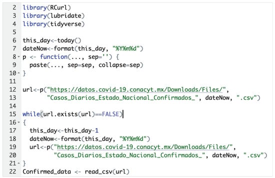
Figure 1. Code to read the data from the official website.

However, this dataset contains the daily reported COVID-19 infections, which is unstable due to the frequency of reporting cases in Mexico, as shown in Figure 2.

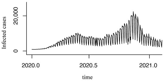
Figure 2. Unstable original time series.

Therefore, we made several tests to identify a minimum size rolling moving average (RMA) that showed a uniform behavior. Finally, we found that seven days of RMA were needed to smooth the time series, as it was also proposed in [14,31], as shown in Equation (1) and Figure 3.

$$tsRM{A}_t=\frac{{\sum }_{i=0}^{6}t{s}_{t+i}}{7}$$

(1)

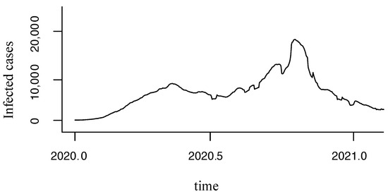
Figure 3. Time series after applying RMA of seven days.

As a general idea, the data extraction methodology can be visualized in Figure 4. The complete dataset is filtered and segmented for the summarized time series (by country) in eight states (federal entities), taking into account the highest population density reported on INEGI’s website with the Population and Housing Census 2020 [32]. The selected states are shown in Figure 5: Ciudad de México, Estado de México, Morelos, Tlaxcala, Aguascalientes, Querétaro, Guanajuato, and Puebla.

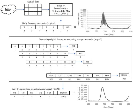
Figure 4. Data extraction methodology.

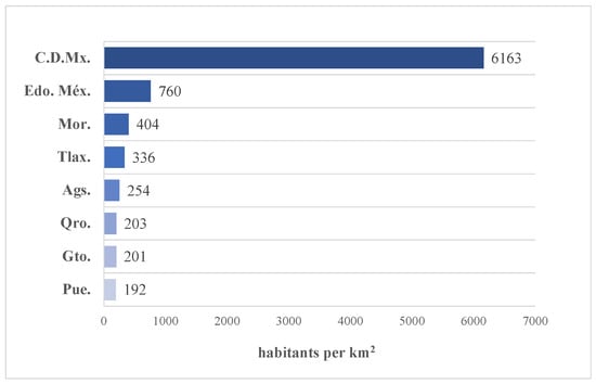
Figure 5. States with the highest population density in Mexico.

3. Dataset Transformation

In previous works [3], we noticed that forecasting techniques struggle when working with small-sized time series; hence, this paper aims to produce a model that can forecast with limited data. Therefore, we decided to transform the $tsRMA$ to a dataset by extracting time windows of size ($ws$) and reorganizing each time window in a dataset row plus one day ahead. Additionally, we try two other transformations for the time series before converting it to a dataset. Finally, we randomly chose 70% of the rows for training and the remainder 30% for testing; see Figure 6.

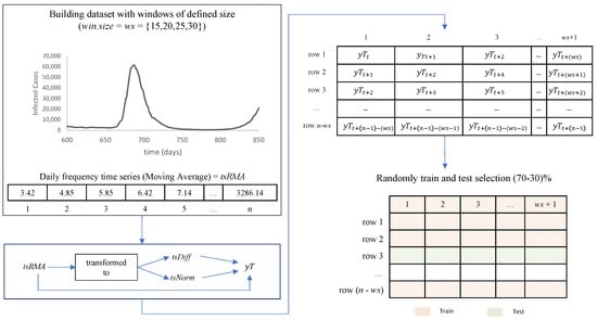
Figure 6. Data transformation methodology.

Here, $tsDiff$ is a differentiated series obtained by extracting the difference between two consecutive values from $tsRMA$ trying to extract the behavior of the time series and not exactly its values (see Equation (2) and Figure 7).

$$tsDif{f}_t=tsRM{A}_{t+1}-tsRM{A}_t$$

(2)

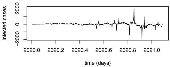
Figure 7. $tsDiff$ time series.

Finally, $tsNorm$ is a normalized transformation that initially normalizes the $tsRMA$ series and then uses a differentiation; the normalization technique is the traditional z-score (see Equations (3) and (4)).

$$\begin{array}{ccc}\hfill nor{m}_t& =& \hfill \frac{tsRM{A}_t-\mu }{\tau }\hfill \end{array}$$

(3)

$$\begin{array}{ccc}\hfill tsNor{m}_t& =& \hfill nor{m}_{t+1}-nor{m}_t\hfill \end{array}$$

(4)

where $\mu$ is the mean of $tsRMA$ series, and $\tau$ is the standard deviation of $tsRMA$.

4. Forecasting Model

In this section, we train a random forest with the training section of the dataset to produce a regression model that can predict one day ahead.

However, this problem requires more than just one day ahead. Therefore, to reach a larger horizon (h), let us say $h=7$, we need to iteratively execute the regression model by shifting the test row to the left and including the newly predicted data in the last column. Figure 8 shows the general methodology of our framework (PGRFF). In this section, we train a random forest with the training section of the dataset to produce a regression model that can predict one day ahead.

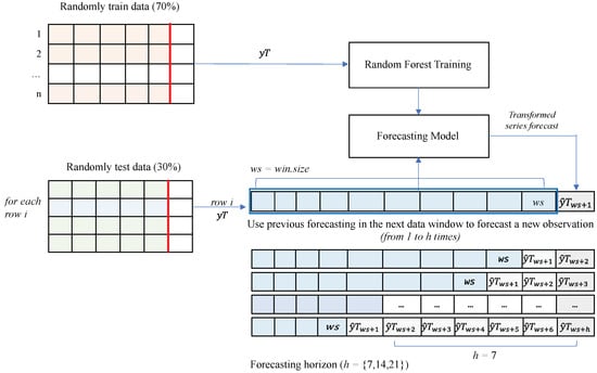
Figure 8. Pandemic random forest-based framework (PRFF).

Once we obtained the forecastings, we evaluated their performance with the symmetric mean average percentage error (sMAPE) as recommended instead of MAPE [33]. However, if $yT$ comes from $tsDiff$ or $tsNorm$, we require to return the values to their original form as the number of infections, see Equations (5) and (6). On the other hand, if $yT$ comes from $tsRMA$, then $\widehat{y}=\widehat{y}T$.

$$\begin{array}{ccc}\hfill \widehat{y}{U}_{t+1}& =& \hfill tsRM{A}_t+\widehat{y}{T}_{t+1}\hfill \end{array}$$

(5)

$$\begin{array}{ccc}\hfill \widehat{y}{U}_{t+k}& =& \hfill \widehat{y}{U}_{t+k-1}+\widehat{y}{T}_{t+k}2\le k\le h\hfill \end{array}$$

(6)

where $\widehat{y}{U}_{t+k}$ is the undifferentiated forecasting at time $t+k$, and $\widehat{y}{U}_{t+1}$ is the first forecasted value. Figure 9 graphically shows the process of Equations (5) and (6).

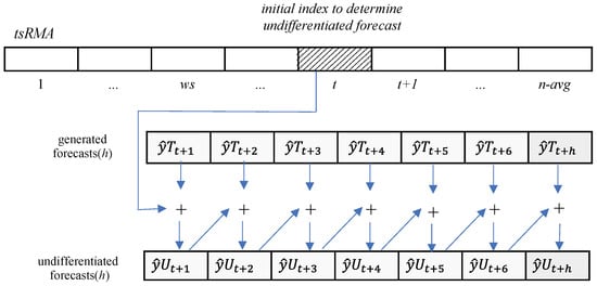
Figure 9. Undifferentiate $\widehat{y}T$ to $\widehat{y}U$.

It is important to highlight that if the original transformed series $yT$ is $tsDiff$, then $\widehat{y}=\widehat{y}U$. On the other hand, if $yT$ is $tsNorm$, we will be further required to denormalize $\widehat{y}U$ to calculate its sMAPE, as shown in Equation (7).

$${\widehat{y}}_{t+k}=(y_{t+k}+\widehat{y}{U}_{t+k})\ast \tau +\mu 1\le k\le h$$

(7)

where $\widehat{y}{U}_{t+k}$ is the forecasting using $tsNorm$ as $yT$ in time ($t+k$), $\mu$ and $\tau$ are the mean and standard deviation of the original $tsRMA$ series, and $\widehat{y}{U}_{t+1}$ is the first forecasted value.

Once we obtain ${\widehat{y}}_{t+k}|1\le k\le h$, which is the forecasting from ($t+1$) to ($t+h$), we can compare the forecasting with the actual data by calculating the sMAPE, as shown in Figure 10.

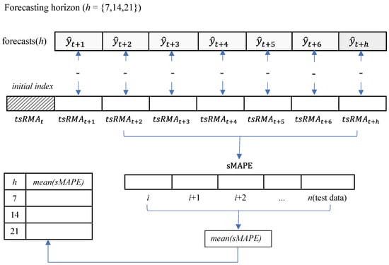
Figure 10. Procedure to calculate the sMAPE, using forecasts undifferentiated.

5. Experimentation Configuration

The experimentation was carried out in an M2 Pro Macbook Pro with 16GB of RAM and 512 GB of SSD running macOS Ventura 13.4.1. Additionally, we use the R framework for the whole process from web mining, forecasting, and graphics production to sMAPE calculation. We produced four forecasting models for windows sizes of 15, 20, 25, and 30 using the $randomForest$ function from the “randomforest” package version 4.6-14 in R version 3.6.1; each model created 500 decision trees.

For the computational experimentation, we use eight time series for the eight Mexican states plus one additional for the whole country.

The final experimentation is according to the parameters in Table 1. Here, PRFF is the pandemic random forest-based framework that trains and forecasts using the same time series. In contrast, PGRFF is a generalized version that trains with the whole country’s time series and forecasts for other time series.

Table 1. Experimental scheme to generate forecast models with the global time series and its application in time series by states.

# $exp$	TS Used	TS Transformation	Forecasting Model
1	Country	tsRMA	PRFF
2	States	tsRMA	PGRFF from exp #1
3	Country	tsDiff	PRFF
4	States	tsDiff	PGRFF from exp #3
5	Country	tsNorm	PRFF
6	States	tsNorm	PGRFF from exp #5

In this experimentation, we focused on developing a model that can be used for little data and trained with the complete time series of the whole country as in $exp$ 2, 4, and 6. To this end, we produced a random forest model for the whole country and tested it with eight Mexican states; we called it a pandemic generalized random forest-based framework (PGRFF). Additionally, we tested the impact on forecasting the dataset window size and horizon size.

6. Results

This section presents the six experiments’ results in Table 1.

Figure 11 shows the best forecasting with PRFF ($exp$ 1) and PGRFF (best state of $exp$ 2). In contrast, Figure 12 shows the worst forecasts with the PRFF model ($exp$ 1) and PGRFF (worst state of $exp$ 2), which is the state of Tlax. Here, we can see that the forecast from Figure 12b) starts high above the actual time series. This behavior occurs because of the high values of the training time series in experiment 1 (country time series). Additionally, the resulting forecast is absolute and is not adjusted to the series in any way.

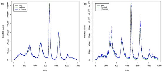
Figure 11. The best forecasting with h = 7 and $ws$ = 15 using $tsRMA$ transformation: (a) time series of whole country from $exp$ 1 and (b) time series of C.D.Mx for $exp$ 2.

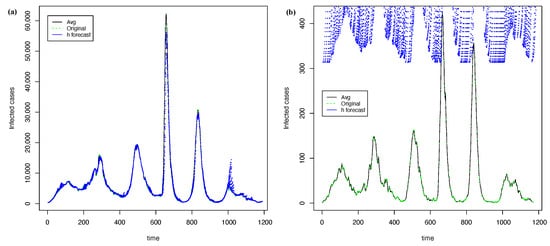
Figure 12. The worst forecasting with h = 21 and $ws$ = 30 using $tsRMA$ transformation: (a) time series of whole country from $exp$ 1 and (b) time series of Tlax for $exp$ 2.

Additionally, in experiment 2, Figure 13 shows the forecasting measure error with h = (7, 14, and 21) from experiment 1. As stated before, the best-performing country was C.D.Mx. In these figures, as a rule of thumb, the larger the horizon (h), the larger the sMAPE. Furthermore, this experiment benefits from small $ws$ values. The best configuration for this experimentation using h = 7 and $ws$ = 15 produced an sMAPE of 156.48.

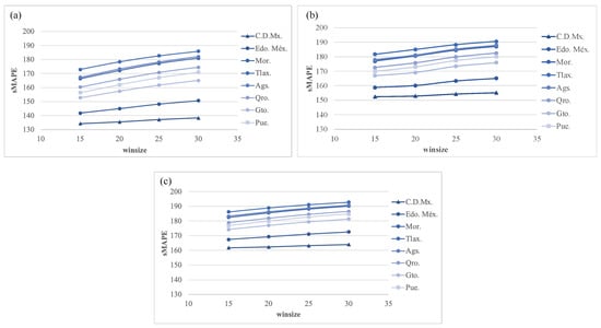
Figure 13. Experiment 2. The best forecasting: sMAPE error using $tsRMA$ transformation for (a) h = 7; (b) h = 14; and (c) h = 21.

Figure 14 shows the best forecasts with PRFF ($exp$ 3) and PGRFF (best state of $exp$ 4). In contrast, Figure 15 shows the worst forecasts with the PRFF ($exp$ 3) and PGRFF (worst state of $exp$ 4), which is the state of Tlax. Here, we can see that the forecasts move straight upward in Figure 15b. This behavior also corresponds to training with the high values of the training time series in experiment 3. However, as $tsDiff$ requires an adjustment to fix the forecast to the original time series, such adjustment notoriously improves over $tsRMA$ transformation in Figure 12b; however, it still has plenty of room for improvement.

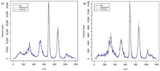
Figure 14. The best forecasting with h = 7 and $ws$ = 15 using $tsDiff$ transformation: (a) time series of whole country from $exp$ 3 (b) time series of C.D.Mx. from $exp$ 4.

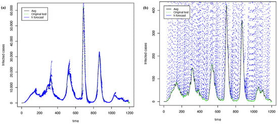
Figure 15. The worst forecasting with h = 21 and $ws$ = 25 using $tsDiff$ transformation: (a) time series of whole country from $exp$ 3 and (b) time series of Tlax from $exp$ 4.

Figure 16 shows the results of experiment 4 with h = (7, 14, and 21) using PGRFF trained from experiment 3 via $tsDiff$ transformation. In this experiment, as well as in $exp$ 2, the best sMAPE was produced with h = 7. However, regarding $ws$, the best configuration was $ws$ = 15, while the worst was $ws$ = 25 instead of 30, as presented in $exp$ 2. The best configuration for this experimentation using h = 7 and $ws$ = 15 produced a sMAPE = 25.48.

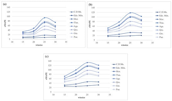
Figure 16. Experiment 4. The best forecasting: sMAPE error using $tsDiff$ transformation for (a) h = 7; (b) h = 14; and (c) h = 21.

Figure 17 shows the best forecasts with PRFF ($exp$ 5) and PGRFF (best state of $exp$ 6). In contrast, Figure 18 shows the worst forecasts presented with PRFF ($exp$ 5) and PGRFF (worst state of $exp$ 6), the state of Tlax. Although the behavior in Figure 18a is worse than Figure 15 and Figure 12a, the performance in Figure 12b visually improves dramatically with $tsNorm$. Therefore, we sacrificed performance in the training time-series $exp$ 5 but improved the robustness of the model for the rest of the states $exp$ 6, which was our main goal.

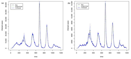
Figure 17. The best forecasting with h = 7 and $ws$ = 25 using $tsNorm$ transformation: (a) time series of whole country from $exp$ 5 and (b) time series of C.D.Mx. from $exp$ 6.

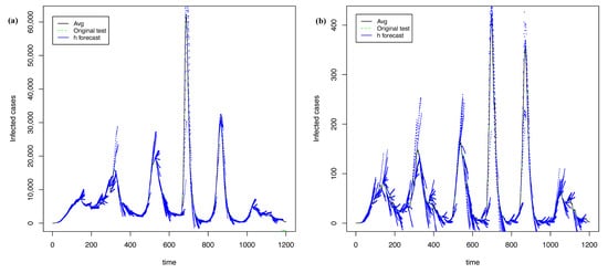
Figure 18. The worst forecasting with h = 21 and $ws$ = 20 using $tsNorm$ transformation: (a) time series of whole country from $exp$ 5 and (b) time series of Tlax from $exp$ 6.

In experiment 6, Figure 19 shows the forecasting measure error with h = (7, 14, and 21) using a PGRFF from experiment 5, transformed using $tsNorm$. In this experiment, as well as in $exp$ 2 and 4, the best sMAPE was produced with h = 7. However, there was a notable change in the behavior of the sMAPE regarding the $ws$; here, the best sMAPE results are obtained with $ws$ = 25, increasing the sMAPE with higher and lower $ws$ values. The best configuration for this experimentation using h = 7 and $ws$ = 25 produced an sMAPE of 13.58.

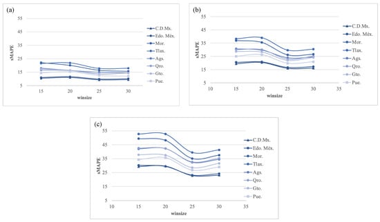
Figure 19. Experiment 6. The best forecasting: sMAPE error using $tsNorm$ transformation for (a) h = 7; (b) h = 14; and (c) h = 21.

Finally, we make a Wilcoxon nonparametric test confirming that $tsNorm$ outperforms statistically to $tsDiff$ and $tsRMA$, with a p_value of 0.012 equivalent to a 98.8% certainty. The test only reached 98.8% because of the limited number of states used.

Comparison with Standard Methods

We carried out two additional experiments to compare the performance of PGRFF against two standards for comparison methods, particularly ETS and ARIMA. As the main objective for this paper is to create a model that can forecast future pandemics in their early stages, for the first additional experiment, we test ETS, ARIMA, and PGRFF with the eight Mexican states and their first one hundred infection days. It is important to note that ETS and ARIMA train with the time series of the eight states, while PGRFF uses a forecasting model trained with the time series of the whole country, $exp$ 6, to forecast the time series of the eight states.

ETS and ARIMA were carried out using functions $auto.arima$ [23] and $ets$ [34] from package “forecast” version 8.16 in R. Figure 20 shows the cumulative sMAPE of ETS, ARIMA, and PGRFF for horizons 7, 14, 21, 28, and 35. Here, we can see that for horizons 7, 14, and 21, ARIMA has the lowest sMAPE, while PGRFF has the highest sMAPE. However, for horizons 28 and 35, PGRFF has the lowest sMAPE, while ETS has the highest sMAPE. Therefore, PGRFF performs better than the standards for comparison methods when forecasting longer horizons.

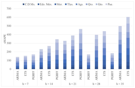
Figure 20. ETS, ARIMA, and PGRFF cumulative sMAPEs comparing.

We use a Wilcoxon nonparametric test to compare ETS, ARIMA, and PGRFF; see Table 2. Here, we can see that the first column contains the horizon size; the second column shows the testing methods where we highlight in red the winning method if there is one; finally, the third and fourth columns show the p_value and percentage of certainty, respectively. However, if the testing methods do not have a significant difference (NSD), we show it in the p_value column.

Table 2. Wilcoxon test for ETS, ARIMA, and PGRFF for one-hundred-day time series.

h	Testing Methods	p_Value	Percentage of Certainty
	ETS vs. ARIMA	0.012	98.8%
7	ETS vs. PGRFF	NSD
	ARIMA vs. PGRFF	NSD
	ETS vs. ARIMA	0.012	98.8%
14	ETS vs. PGRFF	0.05	95%
	ARIMA vs. PGRFF	0.012	98.8%
	ETS vs. ARIMA	0.017	98.3%
21	ETS vs. PGRFF	NSD
	ARIMA vs. PGRFF	0.012	98.8%
	ETS vs. ARIMA	0.025	97.5%
28	ETS vs. PGRFF	0.012	98.8%
	ARIMA vs. PGRFF	0.012	98.8%
	ETS vs. ARIMA	0.012	98.8%
35	ETS vs. PGRFF	0.012	98.8%
	ARIMA vs. PGRFF	0.012	98.8%

Therefore, as we stated before, ARIMA generally produced the best statistical results for horizons 7, 14, and 21. However, for horizons 28 and 35, PGRFF outperformed ETS and ARIMA. It is important to highlight that PGRFF could obtain a more significant percentage of certainty if more time series were used, given its lower sMAPE values.

Furthermore, Figure 21 shows the behavior of ETS, ARIMA, and PGRFF for C.D. Mx with $h=21$ in the first peak of the time series at about 300 days. Here, we can see that ETS and ARIMA produce similar to straight forecastings, while PGRFF produces forecastings with curves that are more similar to the actual time series; however, this behavior is not shown in the sMAPE presented in Table 2.

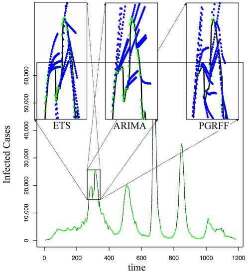
Figure 21. Forecasting C.D.Mx. with h = 21, comparing ETS, ARIMA, and PGRFF.

In the second additional experimentation, we use a complete time series; ETS and ARIMA are executed similarly to the previous experiment; however, instead of using PGRFF, we use PRFF, which generates a model for each of the eight states.

Figure 22 shows the cumulative sMAPE for h = 7, 14, 21, 28, and 35 produced with ETS, ARIMA, and PRFF. The Wilcoxon test for this experimentation showed a p_value of 0.012 in favor of PRFF versus both (ETS and ARIMA), meaning a 98.8% certainty for all horizons.

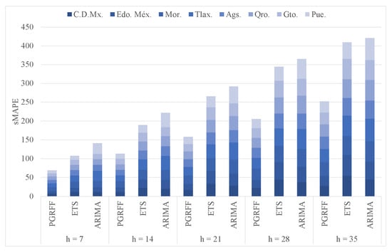
Figure 22. ETS, ARIMA, and PRFF cumulative sMAPEs comparison with the whole infection time series.

7. Discussion

Figure 23 shows that the C.D.Mx. and Tlax. states presented the best and worst sMAPE errors in $exp$ 2, 4, and 6. Here, we can see that the best-performing transformation is $tsNorm$ in the best and worst configurations of the best and worst time series.

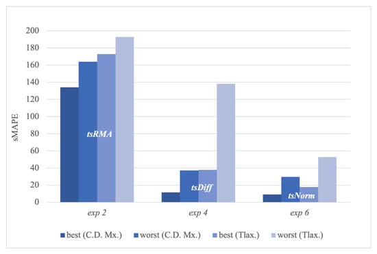
Figure 23. Best and worst sMAPE for C.D.Mx. and Tlax with $tsRMA$, $tsDiff$, and $tsNorm$ transformations.

We proposed the $tsNorm$ transformation to minimize the impact of training a regression model with high-valued time series by normalizing the data. Additionally, the differentiation is also used in $tsNorm$ as a way to fix the starting point of the forecasting near the last-known values of the original time series, avoiding the errors presented in Figure 12b).

We believed the forecastings would fit better for larger $population$ $densities$. However, $exp$ 2, 4, and 6 worked best for states with larger $populations$. Figure 24 compares the $population$ $density$ and $population$ of the eight selected states. It is important to highlight that C.D.Mx. has the best forecasting; however, Edo.Méx is very close to it and can be visualized in Figure 13, Figure 16 and Figure 19.

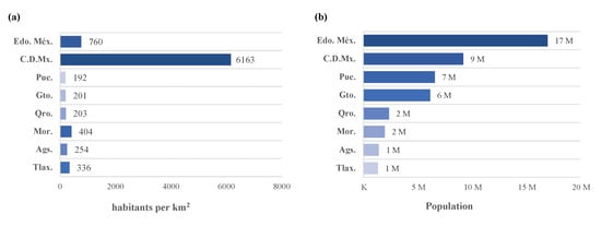
Figure 24. The eight selected states viewed by (a) population density and (b) population.

It is important to highlight that in new pandemics, classical forecastings can only use the current number of observations, and one of the main deficiencies of these methods is that they perform poorly with short time series [3,35].

With this knowledge in mind, we propose PGRFF, which learns from a complete pandemic time series and creates a generalized model that can be used for future pandemics, particularly useful when forecasting pandemic peaks. Additionally, our nongeneralized approach (PRFF) produced better sMAPEs than ETS and ARIMA, showing promising performance even without a pre-trained model; however, we do not consider PRFF as our main contribution because it will lack peak information to forecast such essential moments correctly.

8. Conclusions

This paper proposes a pandemic generalized random forest-based framework PGRFF, which uses current data to produce models to forecast future pandemics. Additionally, we tested three different transformation techniques to produce different forecasting models for COVID-19 time series. We approach this problem considering a limited-sized pandemic time series to produce datasets with small time window observations. Therefore, we develop a model with current pandemic data on COVID-19 from a specific country that can forecast pandemic time series from different states within the country.

As we can see in the experimentation section, the model trained with the $tsNorm$ visually and statistically produced better results than the other two transformation techniques. Additionally, we performed two non-parametric Wilcoxon tests, one between $tsNorm$ and $tsDiff$ and the other between $tsNorm$ and $tsRMA$. These tests statistically proved with a 98.8% certainty that $tsNorm$ outperformed $tsDiff$ and $tsRMA$ with a p-value of 0.012.

When comparing PGRFF with ETS and ARIMA, we found that for larger horizons, PGRFF statistically outperformed ETS and ARIMA, proving that our proposal is better than the standard methods for comparison. Furthermore, we visually showed that PGRFF performed better than ETS and ARIMA in the first peak of the COVID-19 time series because it has information regarding the behavior of the peaks from the country time series, information that ETS and ARIMA could not have.

Contrary to what we believed at the beginning of the experimentation, the forecasts produce better results when the studied states have their population similar to the time series used as training instead of their population density. In future work, we will consider using an intermediate state as training to decrease the differences among the populations of the different states with respect to the training series. We would also like to use larger datasets from other countries while testing artificial neural networks as a regression technique.

Finally, we showed that by preprocessing Mexico’s COVID-19 time series, we could create one model that can be useful to forecast the pandemic time series of other states within the country. We consider this experiment relevant because we can use this approach to produce a trained model to forecast possible future pandemics in their early stages.

References

- Abdalla, S.; Bakhshwin, D.; Shirbeeny, W.; Bakhshwin, A.; Bahabri, F.; Bakhshwin, A.; Alsaggaf, S.M. Successive waves of COVID-19: Confinement effects on virus-prevalence with a mathematical model. Eur. J. Med. Res. 2021, 26, 128. [Google Scholar] [CrossRef] [PubMed]
- Cherednik, I. Modeling the Waves of COVID-19. Acta Biotheor. 2022, 70, 8. [Google Scholar] [CrossRef] [PubMed]
- Cruz-Nájera, M.A.; Treviño-Berrones, M.G.; Ponce-Flores, M.P.; Terán-Villanueva, J.D.; Castán-Rocha, J.A.; Ibarra-Martínez, S.; Santiago, A.; Laria-Menchaca, J. Short Time Series Forecasting: Recommended Methods and Techniques. Symmetry 2022, 14, 1231. [Google Scholar] [CrossRef]
- Aguilar-Madera, C.G.; Espinosa-Paredes, G.; Herrera-Hernández, E.C.; Briones Carrillo, J.A.; Valente Flores-Cano, J.; Matías-Pérez, V. The spreading of COVID-19 in Mexico: A diffusional approach. Results Phys. 2021, 27, 104555. [Google Scholar] [CrossRef]
- El Aferni, A.; Guettari, M.; Tajouri, T. Mathematical model of Boltzmann’s sigmoidal equation applicable to the spreading of the coronavirus (COVID-19) waves. Environ. Sci. Pollut. Res. 2021, 28, 40400–40408. [Google Scholar] [CrossRef]
- He, S.; Tang, S.; Rong, L. A discrete stochastic model of the COVID-19 outbreak: Forecast and control. Math. Biosci. Eng. 2020, 17, 2792–2804. [Google Scholar] [CrossRef]
- Darti, I.; Suryanto, A.; Panigoro, H.S.; Susanto, H. Forecasting COVID-19 Epidemic in Spain and Italy Using A Generalized Richards Model with Quantified Uncertainty. Commun. Biomath. Sci. 2020, 3, 90–100. [Google Scholar] [CrossRef]
- Drews, M.; Kumar, P.; Singh, R.K.; De La Sen, M.; Singh, S.S.; Pandey, A.K.; Kumar, M.; Rani, M.; Srivastava, P.K. Model-based ensembles: Lessons learned from retrospective analysis of COVID-19 infection forecasts across 10 countries. Sci. Total Environ. 2022, 806, 150639. [Google Scholar] [CrossRef]
- Kamley, S. Comparative Study of Various Data Mining Techniques Towards Analysis and Prediction of Global COVID-19 Dataset. In Machine Learning for Healthcare Applications; Mohanty, S.N., Nalinipriya, G., Jena, O.P., Sarkar, A., Eds.; Wiley Online Library: Hoboken, NJ, USA, 2021. [Google Scholar] [CrossRef]
- Fard, S.G.; Rahimi, H.M.; Motie, P.; Minabi, M.A.; Taheri, M.; Nateghinia, S. Application of machine learning in the prediction of COVID-19 daily new cases: A scoping review. Heliyon 2021, 7, e08143. [Google Scholar] [CrossRef]
- Dairi, A.; Harrou, F.; Zeroual, A.; Hittawe, M.M.; Sun, Y. Comparative study of machine learning methods for COVID-19 transmission forecasting. J. Biomed. Inform. 2021, 118, 103791. [Google Scholar] [CrossRef]
- Chandra, R.; Jain, A.; Chauhan, D.S. Deep learning via LSTM models for COVID-19 infection forecasting in India. PLoS ONE 2022, 17, 1–28. [Google Scholar] [CrossRef]
- Masum, M.; Masud, M.A.; Adnan, M.I.; Shahriar, H.; Kim, S. Comparative study of a mathematical epidemic model, statistical modeling, and deep learning for COVID-19 forecasting and management. Socio-Econ. Plan. Sci. 2022, 80, 101249. [Google Scholar] [CrossRef]
- Pavlyutin, M.; Samoyavcheva, M.; Kochkarov, R.; Pleshakova, E.; Korchagin, S.; Gataullin, T.; Nikitin, P.; Hidirova, M. COVID-19 Spread Forecasting, Mathematical Methods vs. Machine Learning, Moscow Case. Mathematics 2022, 10, 195. [Google Scholar] [CrossRef]
- Makridakis, S.; Spiliotis, E.; Assimakopoulos, V. The M4 Competition: 100,000 time series and 61 forecasting methods. Int. J. Forecast. 2020, 36, 54–74. [Google Scholar] [CrossRef]
- Brown, R.G. Statistical Forecasting for Inventory Control; McGraw-Hill: New York, NY, USA, 1959; p. 1959. [Google Scholar]
- Holt, C.C. Forecasting seasonals and trends by exponentially weighted moving averages. Int. J. Forecast. 2004, 20, 5–10. [Google Scholar] [CrossRef]
- Winters, P.R. Forecasting Sales by Expoentially Weighted Moving Averages. In Lecture Notes in Economics and Mathematical Systems; Springer: Berlin/Heidelberg, Germany, 1960; Volume 132, pp. 324–342. [Google Scholar] [CrossRef]
- Hyndman, R.J.; Koehler, A.B.; Snyder, R.D.; Grose, S. A state space framework for automatic forecasting using exponential smoothing methods. Int. J. Forecast. 2002, 18, 439–454. [Google Scholar] [CrossRef]
- Ospina, R.; Gondim, J.A.; Leiva, V.; Castro, C. An Overview of Forecast Analysis with ARIMA Models during the COVID-19 Pandemic: Methodology and Case Study in Brazil. Mathematics 2023, 11, 3069. [Google Scholar] [CrossRef]
- Kaur, J.; Parmar, K.S.; Singh, S. Autoregressive models in environmental forecasting time series: A theoretical and application review. Environ. Sci. Pollut. Res. 2023, 30, 19617–19641. [Google Scholar] [CrossRef]
- Rahman, M.S.; Chowdhury, A.H.; Amrin, M. Accuracy comparison of ARIMA and XGBoost forecasting models in predicting the incidence of COVID-19 in Bangladesh. PLoS Glob. Public Health 2022, 2, e0000495. [Google Scholar] [CrossRef]
- Hyndman, R.J.; Khandakar, Y. Automatic time series forecasting: The forecast package for R. J. Stat. Softw. 2008, 27, 1–22. [Google Scholar] [CrossRef]
- Ho, T.K. Random decision forests. In Proceedings of the 3rd International Conference on Document Analysis and Recognition, Montreal, QC, Canada, 14–16 August 1995; Volume 1, pp. 278–282. [Google Scholar] [CrossRef]
- Breiman, L. Random Forests. Mach. Learn. 2001, 45, 5–32. [Google Scholar] [CrossRef]
- Vaughan, L.; Zhang, M.; Gu, H.; Rose, J.B.; Naughton, C.C.; Medema, G.; Allan, V.; Roiko, A.; Blackall, L.; Zamyadi, A. An exploration of challenges associated with machine learning for time series forecasting of COVID-19 community spread using wastewater-based epidemiological data. Sci. Total Environ. 2023, 858, 159748. [Google Scholar] [CrossRef] [PubMed]
- Castán-Lascorz, M.A.; Jiménez-Herrera, P.; Troncoso, A.; Asencio-Cortés, G. A new hybrid method for predicting univariate and multivariate time series based on pattern forecasting. Inf. Sci. 2022, 586, 611–627. [Google Scholar] [CrossRef]
- Chumachenko, D.; Meniailov, I.; Bazilevych, K.; Chumachenko, T.; Yakovlev, S. Investigation of Statistical Machine Learning Models for COVID-19 Epidemic Process Simulation: Random Forest, K-Nearest Neighbors, Gradient Boosting. Computation 2022, 10, 86. [Google Scholar] [CrossRef]
- Masini, R.P.; Medeiros, M.C.; Mendes, E.F. Machine learning advances for time series forecasting. J. Econ. Surv. 2023, 37, 76–111. [Google Scholar] [CrossRef]
- CONAHCYT. COVID-19 Tablero México-CONACYT-CentroGeo-GeoInt-DataLab. Available online: https://datos.COVID-19.conacyt.mx/#DownZCSV (accessed on 5 January 2023).
- Srivastava, S.R.; Meena, Y.K.; Singh, G. Forecasting on COVID-19 infection waves using a rough set filter driven moving average models. Appl. Soft Comput. 2022, 131, 109750. [Google Scholar] [CrossRef]
- Gobierno de México, I. Cuéntame de México/Densidad de población. 2022. Available online: https://cuentame.inegi.org.mx/poblacion/densidad.aspx?tema=P (accessed on 4 August 2022).
- Hyndman, R.J.; Koehler, A.B. Another look at measures of forecast accuracy. Int. J. Forecast. 2006, 22, 679–688. [Google Scholar] [CrossRef]
- Hyndman, P.R.; Koehler, P.A.; Ord, P.K.; Snyder, A.P.R. Forecasting with Exponential Smoothing; Springer: Berlin/Heidelberg, Germany, 2008; pp. 1–356. [Google Scholar]
- Palivonaite, R.; Lukoseviciute, K.; Ragulskis, M. Short-term time series algebraic forecasting with mixed smoothing. Neurocomputing 2016, 171, 854–865. [Google Scholar] [CrossRef]
Disclaimer/Publisher’s Note: The statements, opinions and data contained in all publications are solely those of the individual author(s) and contributor(s) and not of MDPI and/or the editor(s). MDPI and/or the editor(s) disclaim responsibility for any injury to people or property resulting from any ideas, methods, instructions or products referred to in the content. |
© 2023 by the authors. Licensee MDPI, Basel, Switzerland. This article is an open access article distributed under the terms and conditions of the Creative Commons Attribution (CC BY) license (https://creativecommons.org/licenses/by/4.0/).