Distributionally Robust Reinsurance with Glue Value-at-Risk and Expected Value Premium

Abstract

In this paper, we explore a distributionally robust reinsurance problem that incorporates the concepts of Glue Value-at-Risk and the expected value premium principle. The problem focuses on stop-loss reinsurance contracts with known mean and variance of the loss. The optimization problem can be formulated as a minimax problem, where the inner problem involves maximizing over all distributions with the same mean and variance. It is demonstrated that the inner problem can be represented as maximizing either over three-point distributions under some mild condition or over four-point distributions otherwise. Additionally, analytical solutions are provided for determining the optimal deductible and optimal values.

1. Introduction

Reinsurance has played a crucial role in facilitating the transfer of risks from insurers to reinsurers. The optimization of reinsurance strategies has been the subject of extensive research, with significant contributions made by [1,2]. Since then, numerous extensions and advancements have been proposed in this field.

Some researchers have devoted their attention to identifying the most favorable reinsurance contract through the examination of multiple criteria. These criteria encompass minimizing regulatory capital and mitigating the insurer’s risk exposure with respect to specific risk measures. The first proposal of the optimal reinsurance problem for VaR and CVaR risk measures was put forward by [3]. They analyzed the class of stop-loss policies based on the expected value premium principle. Ref. [4] expanded the scope of optimal reinsurance selection to a broader set. Additionally, Refs. [5,6,7] have investigated various approaches and models to determine the optimal reinsurance contract in accordance with the selected risk measure. For a comprehensive overview of optimal reinsurance design with a focus on risk measures, we highly recommend consulting the survey paper [8].

Given the practical difficulties in obtaining the precise distribution of losses, a widely adopted approach to tackle model uncertainty is the utilization of a moment-based uncertainty set. This approach entails considering distributions that adhere to particular moment constraints. An example of this is seen in [9], where optimal reinsurance incorporating stop-loss contracts was examined while accounting for incomplete information regarding the loss distribution. In a similar vein, Ref. [10] examined model uncertainty in the insurance context by maximizing over a finite set of probability measures. In the research conducted in [11], the investigation of VaR-based and CVaR-based reinsurance took place, while taking into account model uncertainty related to stop-loss reinsurance contracts. The authors successfully provided an analytical solution to the reinsurance problem. Moreover, in the study conducted in [12], a distributionally robust reinsurance problem incorporating expectiles was examined, and the optimization problem was numerically solved.

In this paper, we investigate a reinsurance problem incorporating the risk measure Glue Value-at-Risk (GlueVaR) under the framework of distributional robustness. GlueVaR, initially introduced in [13] as a function with four parameters, enables the customization of risk measures to specific contexts by adjusting these parameters. The practical aspects of tail-subadditivity were analyzed by the authors of [14], who also examined the subadditivity and tail-subadditivity of risk aggregation. In a recent study, Ref. [15] examined the optimal reinsurance problem using a novel combination of risk measures and derived closed-form solutions for optimal reinsurance policies. They also explored the application of VaR and GlueVaR as specific instances of risk management. However, it is important to note that their analysis assumed knowledge of the risk distribution. In our research, we possess partial knowledge about the distribution of losses, specifically, regarding the mean and variance. The primary contribution of this paper is to establish that the worst-case distribution falls within the category of three-point or four-point distributions, thereby transforming the infinite-dimensional inner problem into a finite-dimensional one. As a result, we obtain closed-form solutions for the optimal deductible and optimal value. Our findings build upon the conclusions presented in [11], thus extending their implications.

The remaining sections of this paper are structured as follows. Section 2 presents the definition and properties of GlueVaR and formulates our distributionally robust reinsurance problem as a minmax problem. In Section 3, we address the distributionally robust reinsurance problem by identifying the optimal deductibles and optimal values. Section 4 provides an in-depth discussion on the optimal solution, and concludes the paper with closing remarks. Some detailed proofs can be found in the Appendix A and Appendix B.

2. Preliminaries

2.1. Risk Measures

A risk measure is a mathematical function that assigns a non-negative real number to a specific level of risk. Within the financial and insurance sectors, two commonly utilized risk measures are Value-at-Risk (VaR) and Conditional Value-at-Risk (CVaR). For a deeper understanding of CVaR, please consult the discussion provided in [16].

For a random variable X, VaR is defined in two versions: left-continuous VaR (${\mathrm{VaR}}^{-}$) and right-continuous VaR (VaR). They are defined as

$${\mathrm{VaR}}_{\alpha }^{-}\left(X\right)=inf\{t\in \mathbb{R}\mid \mathbb{P}(X⩽t)⩾\alpha \},\alpha \in (0,1],$$

and

$${\mathrm{VaR}}_{\alpha }\left(X\right)=inf\{t\in \mathbb{R}\mid \mathbb{P}(X⩽t)>\alpha \},\alpha \in [0,1),$$

respectively. Specifically, let ${\mathrm{VaR}}_0^{-}\left(X\right)={\mathrm{VaR}}_0\left(X\right)$ and ${\mathrm{VaR}}_1\left(X\right)={\mathrm{VaR}}_1^{-}\left(X\right)$. Both of these measures serve as a scientific foundation for determining the initial capital required by a company to withstand risks. However, it should be noted that ${\mathrm{VaR}}^{-}$ and VaR do not satisfy subadditivity, and they cannot accurately calculate extreme risks.

CVaR, also known as expected shortfall, satisfies the property of subadditivity, which was defined as

$${\mathrm{CVaR}}_{\alpha }\left(X\right)=\frac{1}{1-\alpha }{\int }_{\alpha }^1{\mathrm{VaR}}_u^{-}\left(X\right)\mathrm{d}u,\alpha \in [0,1),{\mathrm{CVaR}}_1\left(X\right)={\mathrm{VaR}}_1^{-}\left(X\right),$$

provided the integral exists. Ref. [17] proposed ${\mathrm{RVaR}}_{\alpha ,\beta }$ at levels $0<\alpha <\beta ⩽1$, as follows:

$${\mathrm{RVaR}}_{\alpha ,\beta }\left(X\right)=\frac{1}{\beta -\alpha }{\int }_{\alpha }^{\beta }{\mathrm{VaR}}_u\left(X\right)\mathrm{d}u.$$

RVaR includes right-continuous VaR and CVaR as its limiting cases, and the two versions of VaR do not impact the values of RVaR and CVaR.

Moving on to another perspective, Ref. [18] defines a family of risk measures using the concept of a distortion function. A distortion function is an non-decreasing function $g:[0,1]\to [0,1]$ such that $g\left(0\right)=0$ and $g\left(1\right)=1$. The corresponding distortion risk measure, denoted as ${\rho }_g[·]$, is defined as follows:

$${\rho }_g\left[X\right]={\int }_0^{\infty }g\left(\overline{F}\left(t\right)\right)\mathrm{d}t-{\int }_{-\infty }^0[1-g\left(\overline{F}\left(t\right)\right)]\mathrm{d}t$$

where $\overline{F}\left(t\right)$ is the survival function of X. For a more comprehensive understanding of distortion risk measures, see [19,20].

Ref. [13] introduced GlueVaR, denoted by ${\mathrm{GlueVaR}}_{\alpha ,\beta }^{r_1,r_2}\left(X\right)$, which utilizes a distortion function defined as follows:

$$g_{\alpha ,\beta }^{r_1,r_2}\left(x\right):=\left\{\begin{array}{cc}\frac{r_1}{1-\beta }x,\hfill & \mathrm{if}0⩽x<1-\beta ,\hfill \\ r_1+\frac{r_2-r_1}{\beta -\alpha }[x-(1-\beta )],\hfill & \mathrm{if}1-\beta ⩽x<1-\alpha ,\hfill \\ 1,\hfill & \mathrm{if}1-\alpha ⩽x⩽1,\hfill \end{array}\right.$$

where $\alpha ,\beta \in [0,1]$ such that $\alpha ⩽\beta ,r_1\in [0,1]$ and $r_2\in [r_1,1]$. By [13], GlueVaR can be expressed as

$${\mathrm{GlueVaR}}_{\alpha ,\beta }^{r_1,r_2}={\omega }_1{\mathrm{CVaR}}_{\beta }\left(X\right)+{\omega }_2{\mathrm{CVaR}}_{\alpha }\left(X\right)+{\omega }_3{\mathrm{VaR}}_{\alpha }\left(X\right),$$

(1)

where

$$\left\{\begin{array}{c}{\omega }_1=r_1-\frac{(r_2-r_1)(1-\beta )}{\beta -\alpha },\hfill \\ {\omega }_2=\frac{r_2-r_1}{\beta -\alpha }(1-\alpha ),\hfill \\ {\omega }_3=1-{\omega }_1-{\omega }_2=1-r_2.\hfill \end{array}\right.$$

The GlueVaR family can exhibit great flexibility by imposing appropriate conditions on $r_1$ and $r_2$. For instance, risk managers may choose parameters such that ${\mathrm{VaR}}_{\alpha }\left(X\right)⩽{\mathrm{GlueVaR}}_{\alpha ,\beta }^{r_1,r_2}\left(X\right)⩽{\mathrm{CVaR}}_{\alpha }\left(X\right)$. This implies that GlueVaR has the potential to address the limitation of VaR’s tendency to underestimate risks. On the contrary, unlike CVaR, GlueVaR is not overly conservative. Additionally, it is important to note that GlueVaR encompasses (right-continuous) Value-at-Risk (VaR), Conditional Value-at-Risk (CVaR), and Range Value-at-Risk (RVaR) as specific cases. The corresponding distortion functions for these measures are $g_{\alpha ,\alpha }^{0,0}\left(x\right)$, $g_{\alpha ,\alpha }^{1,1}\left(x\right)$, and $g_{\alpha ,\beta }^{0,1}\left(x\right)$, respectively. The graphs of these distortion functions are clearly illustrated in Figure 1.

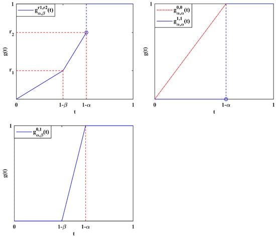
Figure 1. The distortion function of ${\mathrm{GlueVaR}}_{\alpha ,\beta }^{r_1,r_2}$, ${\mathrm{VaR}}_{\alpha }$, ${\mathrm{CVaR}}_{\alpha }$, and ${\mathrm{RVaR}}_{\alpha ,\beta }$: $g_{\alpha ,\beta }^{r_1,r_2}\left(t\right)$, $g_{\alpha ,\alpha }^{0,0}\left(t\right)$, $g_{\alpha ,\alpha }^{1,1}\left(t\right)$, and $g_{\alpha ,\beta }^{0,1}\left(t\right)$.

2.2. Distributionally Robust Reinsurance with GlueVaR

Suppose we have a non-negative ground-up loss, denoted as X, defined on an atomless probability space $(\mathsf{\Omega },\mathcal{F},\mathbb{P})$. The insurer has the option to transfer a portion of the loss, denoted as $I\left(X\right)$, to a reinsurer in exchange for a reinsurance premium, denoted as $\pi \left(I\right(X\left)\right)$. A stop-loss reinsurance contract is defined as $I\left(X\right)={(X-d)}_{+}$, where $d\in [0,\infty ]$ is referred to as the deductible. When $d=0$, the identity function $I\left(X\right)$ is equal to X, which signifies that stop-loss reinsurance defaults to full reinsurance. Conversely, if $d=+\infty$, $I\left(X\right)$ equals 0, indicating that no reinsurance is purchased. In a stop-loss reinsurance arrangement, the total retained loss for the insurer can be expressed as $X-I\left(X\right)+\pi \left(I\left(X\right)\right)=X\wedge d+(1+\theta )\mathbb{E}\left[{(X-d)}_{+}\right]$. Here, $\theta$ denotes a loading factor.

Given a pair of non-negative mean and standard deviation, denoted as $(\mu ,\sigma )$, we define the uncertainty set $\mathcal{F}(\mu ,\sigma )$ as follows:

$$\mathcal{F}(\mu ,\sigma )=\left\{F\mathrm{is}\mathrm{a}\mathrm{cdf}\mathrm{on}[0,\infty ):{\int }_0^{\infty }xdF\left(x\right)=\mu ,{\int }_0^{\infty }{x}^{2}dF\left(x\right)={\mu }^2+{\sigma }^2\right\}.$$

The distributionally robust reinsurance problem based on the risk measure $\rho (·)$ is defined as

$$\underset{d⩾0}{min}\underset{F\in \mathcal{F}(\mu ,\sigma )}{sup}\rho \left(X_F\wedge d+(1+\theta )\mathbb{E}\left[{(X_F-d)}_{+}\right]\right),$$

(2)

where $X_F$ is the loss with distribution function F. An optimal solution to (2) is called an optimal deductible, denoted by $d^{*}$. A distribution that solves

$${\rho }^{\uparrow }\left(d\right):=\underset{F\in \mathcal{F}(\mu ,\sigma )}{sup}\rho \{X_F\wedge d+(1+\theta )\mathbb{E}\left[{(X_F-d)}_{+}\right]\},$$

is referred to as a worst-case distribution, and ${\rho }^{\uparrow }\left(d\right)$ is called the worst-case value corresponding to a given d. In other words, we have ${\rho }^{\uparrow }\left(d^{*}\right)={min}_{d⩾0}{\rho }^{\uparrow }\left(d\right)$.

The distributionally robust reinsurance with $\rho =\mathrm{VaR}$ and $\rho =\mathrm{CVaR}$ has been studied by [11], and when $\rho$ is an expectile-based risk measure, it was studied by [12]. Since GlueVaR can incorporate more information about agents’ attitudes towards risk, we consider the distributionally robust reinsurance problem with GlueVaR. By utilizing the translation invariance of GlueVaR, model (2) can be reduced to

$$\underset{d⩾0}{min}\underset{F\in \mathcal{F}(\mu ,\sigma )}{sup}\{{\mathrm{GlueVaR}}_c(X_F\wedge d)+(1+\theta )\mathbb{E}\left[{(X_F-d)}_{+}\right]\},$$

(3)

where ${\mathrm{GlueVaR}}_c:={\mathrm{GlueVaR}}_{\alpha ,\beta }^{r_1,r_2}$ with $0⩽\alpha ⩽\beta ⩽1$ and $0⩽r_1⩽r_2⩽1$.

From the expression in Equation (1), $\alpha$ and $\beta$ represent the levels of riskiness in GlueVaR. The larger the values of $\alpha$ and $\beta$, the more risk the insurer will transfer to the reinsurer. Conversely, if $\alpha$ and $\beta$ are small enough, the insurer will assume all the risk, aligning with the following proposition.

Proposition 1. 

For $d⩾0$, if the following conditions hold

$$\begin{array}{c}\hfill (1-\alpha )(1+\theta )⩾1,(1-\beta )(1+\theta )⩾r_1,\end{array}$$

(4)

then the optimal deductible for problem (3) is $d^{*}=\infty$.

Proof. 

To demonstrate that $h_c(X_F,d):={\mathrm{GlueVaR}}_c(X_F\wedge d)+(1+\theta )\mathbb{E}\left[{(X_F-d)}_{+}\right]$ is decreasing in $d⩾0$, which implies that ${sup}_{F\in \mathcal{F}(\mu ,\sigma )}{h}_c(X_F,d)$ is decreasing in $d⩾0$, we can use Equations (1) and (3) to obtain the following expression:

$$\begin{array}{cc}\hfill h_c(X_F,d)& ={\omega }_1{\mathrm{CVaR}}_{\beta }(X_F\wedge d)+{\omega }_2{\mathrm{CVaR}}_{\alpha }(X_F\wedge d)+{\omega }_3{\mathrm{VaR}}_{\alpha }(X_F\wedge d)+(1+\theta )\mathbb{E}\left[{(X_F-d)}_{+}\right]\hfill \\ \hfill & =\left(\frac{r_1}{1-\beta }-\frac{r_2-r_1}{\beta -\alpha }\right){\int }_{\beta }^1{\mathrm{VaR}}_u(X_F\wedge d)\mathrm{d}u+\frac{r_2-r_1}{\beta -\alpha }{\int }_{\alpha }^1{\mathrm{VaR}}_u(X_F\wedge d)\mathrm{d}u\hfill \\ \hfill & +(1-r_2){\mathrm{VaR}}_{\alpha }(X_F\wedge d)+(1+\theta )\mathbb{E}\left[{(X_F-d)}_{+}\right].\hfill \end{array}$$

Next, let us consider the following three cases:

(i)

If $d⩽{\mathrm{VaR}}_{\alpha }\left(X\right)$, we have $h_c(X_F,d)=d+(1+\theta )\mathbb{E}\left[{(X_F-d)}_{+}\right]$. Taking the derivative with respect to d, we have

$$h_c^{\prime }(X_F,d)=1-(1+\theta )\overline{F}\left(d\right),$$

From this, we can observe that $h_c^{\prime }(X_F,d)⩽0$. This implies that $h_c(X_F,d)$ is decreasing for $d⩽F^{-1}\left(\frac{\theta }{1+\theta }\right)$, and $h_c(X_F,d)$ is increasing for $d⩾F^{-1}\left(\frac{\theta }{1+\theta }\right)$. Since $(1-\alpha )(1+\theta )⩾1$, it follows that $F^{-1}\left(\frac{\theta }{1+\theta }\right)⩾{\mathrm{VaR}}_{\alpha }\left(X\right)$. Consequently, $h_c(X_F,d)$ is decreasing in $d\in [0,{\mathrm{VaR}}_{\alpha }\left(X\right)]$.

(ii)

If ${\mathrm{VaR}}_{\alpha }\left(X\right)<d⩽{\mathrm{VaR}}_{\beta }\left(X\right)$, which implies $\alpha ⩽F\left(d\right)⩽\beta$, we have

$$\begin{array}{c}\hfill h_c(X_F,d)=d{r}_1+\frac{r_2-r_1}{\beta -\alpha }\left(\beta d-\alpha {\mathrm{VaR}}_{\alpha }\left(X\right)-{\int }_{{\mathrm{VaR}}_{\alpha }}^{d}F\left(t\right)\mathrm{d}t\right),\\ \hfill +(1-r_2){\mathrm{VaR}}_{\alpha }\left(X\right)+(1+\theta )\mathbb{E}\left[{(X_F-d)}_{+}\right].\end{array}$$

Thus, the derivative with respect to d is

$$h_c^{\prime }(X_F,d)=\left(1+\theta -\frac{r_2-r_1}{\beta -\alpha }\right)F\left(d\right)-\left[(1+\theta )-r_1-\frac{(r_2-r_1)\beta }{\beta -\alpha }\right].$$

We will demonstrate that $h_c(X_F,d)$ is decreasing in d by considering the following three subcases.

Subcase 1: $1+\theta >(r_2-r_1)/(\beta -\alpha )$.

In this subcase, $h_c(X_F,d)$ is decreasing for $d⩾0$ if and only if $F\left(d\right)⩽H\left(c\right)$, where

$$H\left(c\right):=\frac{(1+\theta )-r_1-\frac{(r_2-r_1)\beta }{\beta -\alpha }}{1+\theta -\frac{r_2-r_1}{\beta -\alpha }}.$$

By Condition (4), we have $(1-\beta )(1+\theta )⩾r_1/r_2⩾r_1$ and $H\left(c\right)⩾\beta$. Consequently, we can conclude that $F\left(d\right)⩽H\left(c\right)$.

Subcase 2: $1+\theta <(r_2-r_1)/(\beta -\alpha )$.

In this subcase, $h_c(X_F,d)$ is decreasing in $d⩾0$ if and only if $F\left(d\right)⩾H\left(c\right)$. By utilizing condition (4), we can verify that $F\left(d\right)⩾\alpha ⩾H\left(c\right)$.

Subcase 3: $1+\theta =(r_2-r_1)/(\beta -\alpha )$.

In this subcase, we have

$$h_c^{\prime }(X_F,d)=r_1+\frac{(r_2-r_1)\beta }{\beta -\alpha }-(1+\theta )=r_1-(1-\beta )(1+\theta )⩽0.$$

(iii)

If $d⩾{\mathrm{VaR}}_{\beta }\left(X\right)$, then

$$\begin{array}{cc}\hfill h_c(X_F,d)& =\frac{r_1}{1-\beta }d-\frac{r_1}{1-\beta }{\int }_{F^{-1}\left(\beta \right)}^{d}F\left(t\right)\mathrm{d}t+(1+\theta ){\int }_d^{+\infty }\overline{F}\left(t\right)\mathrm{d}t\hfill \\ \hfill & +\frac{r_2-r_1}{\beta -\alpha }{\int }_{\alpha }^{\beta }{\mathrm{VaR}}_u\left(X\right)\mathrm{d}u-\frac{r_1}{1-\beta }\beta F^{-1}\left(\beta \right)+(1-r_2){\mathrm{VaR}}_{\alpha }\left(X\right).\hfill \end{array}$$

From this, we can observe that $h_c^{\prime }(X_F,d)=\left(\frac{r_1}{1-\beta }-(1+\theta )\right)\overline{F}\left(d\right)⩽0$. Therefore, $h_c(X_F,d)$ is decreasing for $d\in [{\mathrm{VaR}}_{\beta }\left(X\right),+\infty )$.

Combining the above three cases, we conclude that $h_c(X_F,d)$ is decreasing for $d⩾0$. □

Noting that ${\mathrm{RVaR}}_{\alpha ,\beta }={\mathrm{GlueVaR}}_{\alpha ,\beta }^{0,1}$, we can derive the following corollary as an immediate consequence of Proposition 1.

Corollary 1. 

If $(1-\alpha )(1+\theta )⩾1$, then the optimal deductible of problem (2) with $\rho ={\mathrm{RVaR}}_{\alpha ,\beta }$ is $d^{*}=\infty$.

3. Main Results

As indicated by Proposition 1, the optimal deductible under certain moderate conditions is $d^{*}=\infty$ for the case where $(1-\alpha )(1+\theta )⩾1$, implying a scenario with no reinsurance purchase. However, practical instances often present $\alpha$ values near 1 and relatively minor $\theta$ values. This makes the condition $(1-\alpha )(1+\theta )>1$ rarely satisfied. Consequently, our primary focus in this section is on cases where $(1-\alpha )(1+\theta )⩽1$.

Moving forward, we employ a methodological approach in examining the issue. In Section 3.1, we transform problem (3) into a finite-dimensional and more computationally amenable problem. Subsequently, in Section 3.2, we deduce the worst-case scenario for problem (5). Lastly, within Section 3.2, we present the optimal deductible for the optimization problem represented by (3).

3.1. The Problem Formulation

We first consider the inner problem of (3), which is defined as follows:

$$h_c^{\uparrow }(X_F,d):=\underset{F\in \mathcal{F}(\mu ,\sigma )}{sup}\{{\mathrm{GlueVaR}}_c(X_F\wedge d)+(1+\theta )\mathbb{E}\left[{(X_F-d)}_{+}\right]\}.$$

(5)

We demonstrate that under mild conditions, if $(1-\alpha )r_1⩽(1-\beta )r_2$, the worst-case distribution of the problem (5) can be restricted to the class of three-point distributions ${\mathcal{F}}_3(\mu ,\sigma )$. Conversely, when $(1-\alpha )r_1⩾(1-\beta )r_2$, the worst-case distribution of problem (5) can be confined to the class of four-point distributions ${\mathcal{F}}_4(\mu ,\sigma )$.

We first present the following two lemmas, which will be utilized in the proof of the subsequent propositions.

Lemma 1. 

For $d⩾0$ and ${\sigma }_1<{\sigma }_2$, let $F=(x_1,\alpha ;x-2,p;x_3,1-\alpha -p)\in {\mathcal{F}}_3(\mu ,{\sigma }_1)$ be a distribution with $x_1<x_2⩽d<x_3$. Suppose $(1-\alpha )r_1⩽(1-\beta )r_2$. Then there exists $F^{*}\in {\mathcal{F}}_3(\mu ,{\sigma }_2)$ such that

$$h_c(X_{F^{*}},d)⩾h_c(X_F,d),0⩽\alpha ⩽\beta ⩽1,0⩽r_1⩽r_2⩽1.$$

Similar to the proof of Lemma 1, we can obtain the following Lemma.

Lemma 2. 

For $d⩾0,{\sigma }_1<{\sigma }_2$, let $F=(x_1,\alpha ;x_2,\beta -\alpha ;x_3,p_3;x_4,p_4)\in {\mathcal{F}}_4(\mu ,{\sigma }_1)$ with $0⩽x_1<x_2<x_3⩽d<x_4$ and $p_3+p_4=1-\beta$. There exists $F^{*}\in {\mathcal{F}}_4(\mu ,{\sigma }_2)$ such that

$$h_c(X_{F^{*}},d)⩾h_c(X_F,d),0⩽\alpha ⩽\beta ⩽1,0⩽r_1⩽r_2⩽1.$$

The next proposition states that if $(1-\alpha )r_1⩽(1-\beta )r_2$, then the worst-case distribution of optimization problem (5) can be limited to the set of three-point distributions ${\mathcal{F}}_3(\mu ,\sigma )$.

Proposition 2. 

Suppose $d⩾0$ and $(1-\alpha )r_1⩽(1-\beta )r_2$. The optimization problem (5) is equivalent to

$$\begin{array}{c}\hfill \underset{F\in {\mathcal{F}}_3(\mu ,\sigma )}{sup}\{{\mathrm{GlueVaR}}_c(X_F\wedge d)+(1+\theta )\mathbb{E}\left[{(X_F-d)}_{+}\right]\}.\end{array}$$

(6)

Proof. 

It suffices to show that for each $F\in \mathcal{F}(\mu ,\sigma )$, there exists a distribution $\tilde{F}\in {\mathcal{F}}_3(\mu ,\sigma )$ such that $h_c(X_{\tilde{F}},d)⩾h_c(X_F,d)$. One can verify that

$$\begin{array}{c}\hfill h_c(X,d)=\left\{\begin{array}{cc}{\mathrm{GlueVaR}}_c(X\wedge d)+(1+\theta )\mathbb{E}\left[{(X-d)}_{+}\right],\hfill & \mathrm{if}d⩾{\mathrm{VaR}}_{\alpha }\left(X\right),\hfill \\ d+(1+\theta )\mathbb{E}\left[{(X-d)}_{+}\right],\hfill & \mathrm{if}d<{\mathrm{VaR}}_{\alpha }\left(X\right).\hfill \end{array}\right.\end{array}$$

To construct $\tilde{F}$, we consider the following three cases.

(i)

If ${\mathrm{VaR}}_{\beta }\left(X\right)⩽d$, let $U\sim U[0,1]$ be a uniform random variable such that U and X are comonotonic. Let $A_1=\{U⩽\alpha \}$, $A_2=\{U>\alpha ,X⩽d\},A_3=\{X>d\}$. Denote ${\mathbb{E}}^F[X\mid A_i]$ by $x_i$ for $i=1,2,3$. Define a discrete random variable

$$\begin{array}{c}\hfill \tilde{X}\left(\omega \right)=\left\{\begin{array}{cc}{x}_1,\hfill & \mathrm{if}\omega \in A_1,\hfill \\ x_2,\hfill & \mathrm{if}\omega \in A_2,\hfill \\ x_3,\hfill & \mathrm{if}\omega \in A_3.\hfill \end{array}\right.\end{array}$$

(7)

We state that $\mathbb{E}\left[\tilde{X}\right]=\mu ,\mathrm{Var}\left(\tilde{X}\right)⩽{\sigma }^2$ and $h_c({\tilde{X}}_{\tilde{F}},d)⩾h_c(X_F,d)$. Indeed, $\mathbb{E}\left[\tilde{X}\right]=\mu =\mathbb{E}\left[X\right]$ obviously holds. Using Hölder’s inequality, we obtain that

$$\mathbb{E}\left[{\tilde{X}}^2\right]=\sum _{i=1}^3\frac{1}{P\left(A_i\right)}{\left({\int }_{A_i}x\mathrm{d}P\left(\omega \right)\right)}^2⩽\sum _{i=1}^3{\int }_{A_i}{x}^2\mathrm{d}P\left(\omega \right)=\mathbb{E}\left[X^2\right].$$

Hence, $\mathrm{Var}\left(\tilde{X}\right)⩽\mathrm{Var}\left(X\right)={\sigma }^2$. By the definition of $\tilde{X}$ as in (7), we obtain

$${\mathrm{GlueVaR}}_c(\tilde{X}\wedge d)-{\mathrm{GlueVaR}}_c(X\wedge d)=\frac{r_2-r_1}{\beta -\alpha }{J}_1-\frac{r_1}{1-\beta }{J}_2+(1-r_2)J_3$$

with

$$J_1=(\beta -\alpha )x_2-{\int }_{\alpha }^{\beta }{\mathrm{VaR}}_u\left(X\right)\mathrm{d}u,J_2={\int }_{\beta }^{F\left(d\right)}{\mathrm{VaR}}_u\left(X\right)\mathrm{d}u-(F\left(d\right)-\beta )x_2,$$

and $J_3=x_2-{\mathrm{VaR}}_{\alpha }\left(X\right)$. By (7), $x_2=\mathbb{E}[X\mid A_2]⩾\mathbb{E}[X\mid A_2^1]=\frac{1}{\beta -\alpha }{\int }_{\alpha }^{\beta }{\mathrm{VaR}}_u\left(X\right)\mathrm{d}u$, where $A_2^1=\{\alpha <U⩽\beta \}$. Consequently, $J_1⩾0$. In a similar manner, we can confirm that $J_2⩾0$ and $J_3⩾0$. Noting that $(1-\alpha )r_1⩽(1-\beta )r_2$ implies $\frac{r_2-r_1}{\beta -\alpha }⩾\frac{r_1}{1-\beta }$, we conclude that

$$\begin{array}{cc}\hfill & {\mathrm{GlueVaR}}_c(\tilde{X}\wedge d)-{\mathrm{GlueVaR}}_c(X\wedge d)\hfill \\ \hfill & ⩾\frac{r_1}{1-\beta }(J_1-J_2)+(1-r_2)J_3\hfill \\ \hfill & =\frac{r_1}{1-\beta }\left[x_2(F\left(d\right)-\alpha )-{\int }_{\alpha }^{F\left(d\right)}{\mathrm{VaR}}_u\left(X\right)\mathrm{d}u\right]+(1-r_2)(x_2-{\mathrm{VaR}}_{\alpha }\left(X\right))\hfill \\ \hfill & =(1-r_2)(x_2-{\mathrm{VaR}}_{\alpha }\left(X\right))⩾0.\hfill \end{array}$$

The second equality holds because $x_2=\mathbb{E}\left[X\right|A_2]=\frac{1}{F\left(d\right)-\alpha }{\int }_{\alpha }^{F\left(d\right)}{\mathrm{VaR}}_u\left(X\right)\mathrm{d}u$. Combining with $\mathbb{E}\left[{(\tilde{X}-d)}_{+}\right]=\left(\mathbb{E}[X\mid A_3]-d\right)\mathbb{P}\left(A_3\right)={\int }_d^{\infty }(x-d)\mathrm{d}F\left(x\right)=\mathbb{E}\left[{(X-d)}_{+}\right],$ the result $h_c({\tilde{X}}_{\tilde{F}},d)⩾h_c(X_F,d)$ follows. If $\mathrm{Var}\left(\tilde{X}\right)={\sigma }^2$, then $\tilde{F}\in {\mathcal{F}}_3(\mu ,\sigma )$, and $h_c({\tilde{X}}_{\tilde{F}},d)⩾h_c(X_F,d)$. If $\mathrm{Var}\left({\tilde{X}}_{\tilde{F}}\right)<{\sigma }^2$, by Lemma 1, there exists a three-point distribution $F^{*}\in {\mathcal{F}}_3(\mu ,\sigma )$ such that $h_c(d,X_{\widetilde{F^{*}}})⩾h_c({\tilde{X}}_{\tilde{F}},d)⩾h_c(X_F,d)$.

(ii)

If ${\mathrm{VaR}}_{\alpha }\left(X\right)⩽d<{\mathrm{VaR}}_{\beta }\left(X\right)$, let $A_1=\{U⩽\alpha \},A_2=\{U>\alpha ,X⩽d\},A_3^1=\{X>d,U⩽\beta \},A_3^2=\{U>\beta \}$, and $A_3=A_3^1\cup A_3^2=\{X>d\}$. Denote ${\mathbb{E}}^F[X\mid A_i]$ by $x_i,i=1,2,3$. Define a discrete random variable $\tilde{X}\left(\omega \right)$ as in Equation (7). Similar to the proof of (i), it is easy to show $\mathbb{E}\left[\tilde{X}\right]=\mu$, $\mathrm{Var}\left(\tilde{X}\right)⩽{\sigma }^2$, and

$$\begin{array}{cc}\hfill & {\mathrm{GlueVaR}}_c(\tilde{X}\wedge d)-{\mathrm{GlueVaR}}_c(X\wedge d)\hfill \\ \hfill & =\frac{r_2-r_1}{\beta -\alpha }\left[x_2(F\left(d\right)-\alpha )-{\int }_{\alpha }^{F\left(d\right)}{\mathrm{VaR}}_u\left(X\right)\mathrm{d}u\right]+(1-r_2)(x_2-{\mathrm{VaR}}_{\alpha }\left(X\right))\hfill \\ \hfill & =(1-r_2)(x_2-{\mathrm{VaR}}_{\alpha }\left(X\right))⩾0,\hfill \end{array}$$

where the inequality follows from $x_2⩾{\mathrm{VaR}}_{\alpha }\left(X\right)$. Noting that $\mathbb{E}\left[{(\tilde{X}-d)}_{+}\right]=\mathbb{E}\left[{(X-d)}_{+}\right]$, the result $h_c({\tilde{X}}_{\tilde{F}},d)⩾h_c(X_F,d)$ follows. If $\mathrm{Var}\left(\tilde{X}\right)={\sigma }^2$, then $\tilde{F}\in {\mathcal{F}}_3(\mu ,\sigma )$, and $h_c({\tilde{X}}_{\tilde{F}},d)⩾h_c(X_F,d)$. If $\mathrm{Var}\left(\tilde{X}\right)<{\sigma }^2$, by Lemma 1, there exists a three-point distribution $F^{*}\in {\mathcal{F}}_3(\mu ,\sigma )$ such $h_c(X_{\widetilde{F^{*}}},d)⩾h_c({\tilde{X}}_{\tilde{F}},d)⩾h_c(X_F,d)$. Then, the result follows.

(iii)

If ${\mathrm{VaR}}_{\alpha }\left(X\right)>d$, define a two-point random variable

$$\begin{array}{c}\hfill \tilde{X}\left(\omega \right)=\left\{\begin{array}{cc}\mathbb{E}[X\mid X⩽d]=x_1,\hfill & \mathrm{if}X⩽d,\hfill \\ \mathbb{E}[X\mid X>d]=x_2,\hfill & \mathrm{if}X>d.\hfill \end{array}\right.\end{array}$$

(8)

Similar to case (i), we have $\mathbb{E}\left(\tilde{X}\right)=\mu ,\mathrm{Var}\left(\tilde{X}\right)⩽{\sigma }^2$ and $h_c({\tilde{X}}_{\tilde{F}},d)⩾h_c(X_F,d)$. For $\epsilon \in [0,x_1/(1-p)]$, define

$$\begin{array}{c}\hfill X_{\epsilon }=\left\{\begin{array}{cc}{x}_1-\epsilon (1-p),\hfill & \mathrm{if}X⩽d,\hfill \\ x_2+\epsilon p,\hfill & \mathrm{if}X>d,\hfill \end{array}\right.\end{array}$$

where $p:=\mathbb{P}(X⩽d)\in [0,\alpha ]$. Note that $\mathbb{E}\left[X_{\epsilon }\right]=\mu$, $\mathrm{Var}\left(X_{\epsilon }\right)$ is continuous and increasing in $\epsilon ⩾0$. Next, we consider the following two subcases.

(iii.a)

If there exists an $\epsilon \in [0,x_1/(1-p)]$ such that $\mathrm{Var}\left(X_{\epsilon }\right)={\sigma }^2$, then the distribution of $X_{\epsilon }$ is the desired two-point distribution.

(iii.b)

Otherwise, we have $\mathrm{Var}\left(X_{{\epsilon }_0}\right)<{\sigma }^2$ with ${\epsilon }_0:=x_1/(1-p)$. In this case, for $q\in [0,1-p]$, we define

$$X^q=(0,p;d,q;y,1-p-q)$$

(9)

with $y:=(\mu -dq)/(1-p-q)>d$. Then $X^0$ and $X_{{\epsilon }_0}$ have the same distribution and $\mathbb{E}{X}^q=\mu ,h_c(d,X^q)⩾h_c(d,X_{{\epsilon }_0})$. Noting that the variance $\mathrm{Var}\left(X^q\right)$ is continuous in $q\in [0,1-p]$ and ${lim}_{q\to 1-p}\mathrm{Var}\left(X^q\right)=\infty$, there exists an $q^{*}\in [0,1-p]$ such that $\mathrm{Var}\left(X^{q^{*}}\right)={\sigma }^2$. Then the distribution of $X^{q^{*}}$ is the desired distribution $F^{*}$.

□

Since ${\mathrm{GlueVaR}}_{\alpha ,\beta }^{0,1}\left(X\right)={\mathrm{RVaR}}_{\alpha ,\beta }\left(X\right)$, we derive the following results for $\mathrm{RVaR}$ from the proof of Proposition 2. These results generalize Proposition 1 in [11].

Corollary 2. 

For $d⩾0$, we have

$$\underset{F\in \mathcal{F}(\mu ,\sigma )}{sup}\{\mathrm{RVaR}(X_F\wedge d)+(1+\theta )\mathbb{E}\left[{(X_F-d)}_{+}\right]\}=\underset{F\in {\mathcal{F}}_3(\mu ,\sigma )}{sup}\{\mathrm{RVaR}(X_F\wedge d)+(1+\theta )\mathbb{E}\left[{(X_F-d)}_{+}\right]\}$$

From the proof of Proposition 2, we can obtain the explicit form of the worst-case distributions. Specifically, we have the following result as a corollary of Proposition 2.

Corollary 3. 

For $d⩾0$, if $(1-\alpha )r_1⩽(1-\beta )r_2$, the worst-case distribution $F=(x_1,p_1;x_2,p_2;x_3,p_3)\in {\mathcal{F}}_3(\mu ,\sigma )$ of problem (5) must be in the following two sets:

$${\mathcal{F}}_2^{\wedge }(\mu ,\sigma ;d):=\{(x_1,p_1;x_2,p_2)\in \mathcal{F}(\mu ,\sigma ):p_1⩽\alpha ,x_1⩽d<x_2\},$$

$${\mathcal{F}}_3^{\wedge }(\mu ,\sigma ;d):=\{(x_1,\alpha ;x_2,p_2;x_3,p_3)\in \mathcal{F}(\mu ,\sigma ):x_1⩽x_2⩽d⩽x_3\}.$$

Proof. 

In the proof of Proposition 2 case (iii.b), for the $X^{q^{*}}$ founded in the proof, we consider the following three cases.

(i)

If $q^{*}>\beta -p$, then ${\mathrm{VaR}}_{\beta }\left(X^{q^{*}}\right)=d$. By applying case (i) of the proof of Proposition 2, we obtain a three-point distribution in ${\mathcal{F}}_3^{\wedge }(\mu ,\sigma ;d)$.

(ii)

If $\alpha -p<q^{*}⩽\beta -p$, then ${\mathrm{VaR}}_{\alpha }\left(X^{q^{*}}\right)=d$ if $p⩽\alpha$, ${\mathrm{VaR}}_{\alpha }\left(X^{q^{*}}\right)=0$ if $p>\alpha$, and ${\mathrm{VaR}}_{\beta }\left(X^{q^{*}}\right)=y>d$. In this case, by applying case (ii) of the proof of Proposition 2, we obtain a three-point distribution in ${\mathcal{F}}_3^{\wedge }(\mu ,\sigma ;d)$.

(iii)

If $q^{*}⩽\alpha -p$, then ${\mathrm{VaR}}_{\alpha }\left(X^{q^{*}}\right)=y>d$. In this case, we can apply case (iii) of the proof of Proposition 2. Specifically, we obtain a random variable $X^{q_1}$ defined by (9) with $q_1+p_1>q^{*}+p$. By iterating this process, we can obtain a distribution in case (i), (ii), or case (iii.a) of the proof of Proposition 2, such that the objective function $h_c(X,d)$ is not less than that of the original one.

□

The proposition below asserts that if $(1-\alpha )r_1⩾(1-\beta )r_2$, then the worst-case distribution of optimization problem (5) can be limited to the set of four-point distributions ${\mathcal{F}}_4(\mu ,\sigma )$.

Proposition 3. 

For $d⩾0$, we assume that $(1-\alpha )r_1⩾(1-\beta )r_2$. The optimization problem (5) can be equivalently represented as follows:

$$\begin{array}{c}\hfill \underset{F\in {\mathcal{F}}_4(\mu ,\sigma )}{sup}\{{\mathrm{GlueVaR}}_c(X_F\wedge d)+(1+\theta )\mathbb{E}\left[{(X_F-d)}_{+}\right]\}.\end{array}$$

(10)

Proof. 

To prove this, it is sufficient to demonstrate that for every $F\in \mathcal{F}(\mu ,\sigma )$, there exists a distribution $\tilde{F}\in {\mathcal{F}}_4(\mu ,\sigma )$ such that $h_c(d,X_{\tilde{F}})⩾h_c(d,X_F)$. We can derive the following expression:

$$\begin{array}{c}\hfill h_c(X,d)=\left\{\begin{array}{cc}{\mathrm{GlueVaR}}_c(X\wedge d)+(1+\theta )\mathbb{E}\left[{(X-d)}_{+}\right],\hfill & \mathrm{if}d⩾{\mathrm{VaR}}_{\alpha }\left(X\right)\hfill \\ d+(1+\theta )\mathbb{E}\left[{(X-d)}_{+}\right],\hfill & \mathrm{if}d<{\mathrm{VaR}}_{\alpha }\left(X\right).\hfill \end{array}\right.\end{array}$$

To construct $\tilde{F}$, we consider the following three cases.

(i)

If ${\mathrm{VaR}}_{\beta }\left(X\right)⩽d$, let $U\sim U[0,1]$ be a uniform random variable that is comonotonic with X. Define the events $A_1=\{U⩽\alpha \}$, $A_2=\{\alpha <U⩽\beta \}$, $A_3=\{U>\beta ,X⩽d\}$, and $A_4=\{X>d\}$. Denote ${\mathbb{E}}^F[X\mid A_i]$ by $x_i$ for $i=1,2,3,4$. We define a discrete random variable as follows:

$$\begin{array}{c}\hfill \tilde{X}\left(\omega \right)=\left\{\begin{array}{cc}{x}_1,\hfill & \mathrm{if}\omega \in A_1,\hfill \\ x_2,\hfill & \mathrm{if}\omega \in A_2,\hfill \\ x_3,\hfill & \mathrm{if}\omega \in A_3,\hfill \\ x_4,\hfill & \mathrm{if}\omega \in A_4.\hfill \end{array}\right.\end{array}$$

(11)

It can be stated that $\mathbb{E}\left[\tilde{X}\right]=\mu$, $\mathrm{Var}\left(\tilde{X}\right)⩽{\sigma }^2$, and $h_c({\tilde{X}}_{\tilde{F}},d)⩾h_c(X_F,d)$. By applying the Hölder inequality, we obtain that

$$\mathbb{E}\left[{\tilde{X}}^2\right]=\sum _{i=1}^4\frac{1}{P\left(A_i\right)}{\left({\int }_{A_i}x\mathrm{d}F\left(x\right)\right)}^2⩽\sum _{i=1}^4{\int }_{A_i}{x}^2\mathrm{d}F\left(x\right)=\mathbb{E}\left[X^2\right].$$

Thus, $\mathrm{Var}\left(\tilde{X}\right)⩽\mathrm{Var}\left(X\right)={\sigma }^2$. From the definition of $\tilde{X}$, it follows that

$$\begin{array}{cc}\hfill & {\mathrm{GlueVaR}}_c(\tilde{X}\wedge d)-{\mathrm{GlueVaR}}_c(X\wedge d)\hfill \\ \hfill & =\frac{r_1}{1-\beta }\left[(F\left(d\right)-\beta )x_3-{\int }_{\beta }^{F\left(d\right)}{\mathrm{VaR}}_u\left(X\right)\mathrm{d}u\right]+\frac{r_2-r_1}{\beta -\alpha }\left[(\beta -\alpha )x_2-{\int }_{\alpha }^{\beta }{\mathrm{VaR}}_u\left(X\right)\mathrm{d}u\right]\hfill \\ \hfill & +(1-r_2)(x_2-{\mathrm{VaR}}_{\alpha }\left(X\right))⩾0.\hfill \end{array}$$

Since

$$\mathbb{E}\left[{(\tilde{X}-d)}_{+}\right]=\left(x_4-d\right)\mathbb{P}\left(A_4\right)={\int }_d^{+\infty }(x-d)dF\left(x\right)=\mathbb{E}\left[{(X-d)}_{+}\right],$$

it follows that $h_c({\tilde{X}}_{\tilde{F}},d)⩾h_c(X_F,d)$.

If $\mathrm{Var}\left(\tilde{X}\right)={\sigma }^2$, then $\tilde{F}\in {\mathcal{F}}_4(\mu ,\sigma )$, and $h_c({\tilde{X}}_{\tilde{F}},d)⩾h_c(X_F,d)$. If ${\mathrm{Var}}^{\tilde{F}}\left(\tilde{X}\right)<{\sigma }^2$, by Lemma 2, there exists a four-point distribution $F^{*}\in {\mathcal{F}}_4(\mu ,\sigma )$ such that $\mathbb{E}\left[{(X_{F^{*}}-d)}_{+}\right]=\mathbb{E}\left[{(X_{\tilde{F}}-d)}_{+}\right]=\mathbb{E}\left[{(X_F-d)}_{+}\right]$ and ${\mathrm{GlueVaR}}_c(X_{F^{*}}\wedge d)⩾{\mathrm{GlueVaR}}_c(X_{\tilde{F}}\wedge d)⩾{\mathrm{GlueVaR}}_c(X_F\wedge d)$. Thus, we have $h_c(X_{\widetilde{F^{*}}},d)⩾h_c({\tilde{X}}_{\tilde{F}},d)⩾h_c(X_F,d)$.

(ii)

If ${\mathrm{VaR}}_{\alpha }\left(X\right)⩽d<{\mathrm{VaR}}_{\beta }\left(X\right)$, let $U\sim U[0,1]$ be comonotonic with X. Let $A_1=\{U⩽\alpha \},A_2=\{\alpha <U,X⩽d\},A_3=\{X>d\}$. Denote $\mathbb{E}\left[X_F\right|A_i]$ by $x_i$ for $i=1,2,3$. Define a discrete random variable $\tilde{X}\left(\omega \right)$ as in (7), and we can determine that $h_c({\tilde{X}}_{\tilde{F}},d)⩾h_c(X_F,d)$.

If $\mathrm{Var}\left(\tilde{X}\right)={\sigma }^2$, then $\tilde{F}\in S_3(\mu ,\sigma )$, and $h_c({\tilde{X}}_{\tilde{F}},d)⩾h_c(X_F,d)$. If $\mathrm{Var}\left({\tilde{X}}_{\tilde{F}}\right)<{\sigma }^2$, by Corollary 2, there exists a three-point distribution $F^{*}\in {\mathcal{F}}_3(\mu ,\sigma )$ such that $h_c(X_{\widetilde{F^{*}}},d)⩾h_c({\tilde{X}}_{\tilde{F}},d)⩾h_c(X_F,d)$.

(iii)

If $d<{\mathrm{VaR}}_{\alpha }\left(X\right)$, the proof is similar to the proof of (iii) in Proposition 2, so we omit it here.

□

3.2. Worst-Case Value

In this subsection, we first present the worst-case value of problem (5) when $(1-\alpha )r_1⩽(1-\beta )r_2$. Subsequently, we derive the worst-case value for $(1-\alpha )r_1⩾(1-\beta )r_2$ as a corollary.

Corollary 3 implies that when $(1-\alpha )r_1⩽(1-\beta )r_2$, we have

$$\begin{array}{cc}\hfill & h^{\uparrow }\left(d\right):=\underset{F\in \mathcal{F}(\mu ,\sigma )}{sup}{h}_c(X_F,d)=max\left\{\underset{F\in {\mathcal{F}}_2^{\wedge }(\mu ,\sigma ;d)}{sup}{h}_c(X_F,d),\underset{F\in {\mathcal{F}}_3^{\wedge }(\mu ,\sigma ;d)}{sup}{h}_c(X_F,d)\right\}.\hfill \end{array}$$

Define ${\mathcal{F}}_3^{\wedge }(\mu ,\sigma ):=\{(x_1,\alpha ;x_2,p_2;x_3,p_3)\in \mathcal{F}(\mu ,\sigma ):x_1⩽x_2⩽x_3\}$. Then, ${\mathcal{F}}_3^{\wedge }(\mu ,\sigma ;d)\subseteq {\mathcal{F}}_3^{\wedge }(\mu ,\sigma )\subseteq {\mathcal{F}}_3(\mu ,\sigma )$, and we can express the supremum as follows:

$$\begin{array}{c}\hfill h_c^{\uparrow }\left(d\right)=max\left\{\underset{F\in {\mathcal{F}}_2^{\wedge }(\mu ,\sigma ;d)}{sup}{h}_c(X_F,d),\underset{F\in {\mathcal{F}}_3^{\wedge }(\mu ,\sigma )}{sup}{h}_c(X_F,d)\right\}.\end{array}$$

(12)

Next, we demonstrate that ${sup}_{F\in {\mathcal{F}}_3^{\wedge }(\mu ,\sigma )}{h}_c(X_F,d)$ is increasing with respect to $\sigma$. This implies that the uncertainty set ${\mathcal{F}}_3^{\wedge }(\mu ,\sigma )$ can be substituted with the following set:

$${\mathcal{F}}_3^{⩽}(\mu ,\sigma ):=\{F\in {\mathcal{F}}_3^{\wedge }(\mu ,{\sigma }_0),{\sigma }_0⩽\sigma \}.$$

Specifically, we can state the following result.

Lemma 3. 

For $d⩾0,\mu ⩾0$, and $\sigma >0$, if $(1-\alpha )r_1⩽(1-\beta )r_2$, we have

$$\begin{array}{c}\hfill h_c^{\uparrow }\left(d\right)=max\left\{\underset{F\in {\mathcal{F}}_2^{\wedge }(\mu ,\sigma ;d)}{sup}{h}_c(X_F,d),\underset{F\in {\mathcal{F}}_3^{★}(\mu ,\sigma ;d)}{sup}{h}_c(X_F,d)\right\},\end{array}$$

(13)

where ${\mathcal{F}}_3^{★}(\mu ,\sigma ;d)$ is any uncertainty set satisfying

$${\mathcal{F}}_3^{\wedge }(\mu ,\sigma ;d)\subseteq {\mathcal{F}}_3^{★}(\mu ,\sigma ;d)\subseteq {\mathcal{F}}_3^{⩽}(\mu ,\sigma ).$$

In the following theorem, we provide the worst-case value for problem (5) under the conditions $(1-\alpha )(1+\theta )⩽1$ and $(1-\alpha )r_1⩽(1-\beta )r_2$.

Theorem 1. 

Let $d⩾0$, for $(1-\alpha )(1+\theta )⩽1$ and $(1-\alpha )r_1⩽(1-\beta )r_2$.

(i)

If $\alpha <{\sigma }^2/({\mu }^2+{\sigma }^2)$, then the worst-case value of problem (5) is

$$h_c^{\uparrow }\left(d\right)=\frac{\mu }{1-\alpha }\wedge d+(1+\theta )(1-\alpha ){\left(\frac{\mu }{1-\alpha }-d\right)}_{+}.$$

(14)

(ii)

If $\alpha ⩾{\sigma }^2/({\mu }^2+{\sigma }^2)$, then the worst-case value of problem (5) is

$$h_c^{\uparrow }\left(d\right)=\left\{\begin{array}{cccc}\hfill & d+(1+\theta )\mu \left(1-\frac{\mu d}{{\mu }^2+{\sigma }^2}\right),\hfill & \hfill & ford⩽d_1,\hfill \\ \hfill & d+\frac{1+\theta }{2}\left[\mu -d+\sqrt{{\sigma }^2+{(\mu -d)}^2}\right],\hfill & \hfill & for{d}_1⩽d⩽d_2,\hfill \\ \hfill & d+(1+\theta )(1-\alpha )\left(\mu -d+\sigma \sqrt{\frac{\alpha }{1-\alpha }}\right),\hfill & \hfill & for{d}_2⩽d⩽d_3,\hfill \\ \hfill & \mu +\sigma \sqrt{\frac{\alpha }{1-\alpha }},\hfill & \hfill & otherwise,\hfill \end{array}\right.$$

(15)

where

$$d_1=\frac{{\mu }^2+{\sigma }^2}{2\mu },d_2=\mu -\sigma \frac{1-2\alpha }{2\sqrt{\alpha (1-\alpha )}},d_3=\mu +\sigma \sqrt{\frac{\alpha }{1-\alpha }}.$$

(16)

Since ${\mathrm{VaR}}_{\alpha }\left(X\right)={\mathrm{GlueVaR}}_{\alpha ,\alpha }^{0,0}$ and ${\mathrm{CVaR}}_{\alpha }\left(X\right)={\mathrm{GlueVaR}}_{\alpha ,\alpha }^{1,1}$, we can derive the following corollary from Theorem 1.

Corollary 4. 

(Mao and Hu, 2022) For $d⩾0,\alpha \in (0,1)$, the worst case value of the following two optimization problems

$$\begin{array}{cc}\hfill & {\mathrm{VaR}}_{\alpha }^{\uparrow }:=\underset{F\in \mathcal{F}(\mu ,\sigma )}{sup}{\mathrm{VaR}}_{\alpha }\{X_F\wedge d+(1+\theta )\mathbb{E}\left[{(X_F-d)}_{+}\right]\}\hfill \\ \hfill & {\mathrm{CVaR}}_{\alpha }^{\uparrow }:=\underset{F\in \mathcal{F}(\mu ,\sigma )}{sup}{\mathrm{CVaR}}_{\alpha }\{X_F\wedge d+(1+\theta )\mathbb{E}\left[{(X_F-d)}_{+}\right]\}\hfill \end{array}$$

equal (14) for $\alpha <{\sigma }^2/({\mu }^2+{\sigma }^2)$, and equal (15) for $\alpha ⩾{\sigma }^2/({\mu }^2+{\sigma }^2)$.

For $\xi \in [0,1]$, let us define the following functions:

$$\begin{array}{cc}\hfill L_1(\xi ,d)& :=\frac{\mu }{1-\xi }\wedge d+(1+\theta )(1-\xi ){\left(\frac{\mu }{1-\xi }-d\right)}_{+},\hfill \\ \hfill L_2\left(d\right)& :=d+(1+\theta )\mu \left(1-\frac{\mu d}{{\mu }^2+{\sigma }^2}\right),\hfill \\ \hfill L_3\left(d\right)& :=d+\frac{1+\theta }{2}\left[\mu -d+\sqrt{{\sigma }^2+{(\mu -d)}^2}\right],\hfill \\ \hfill L_4(\xi ,d)& :=d+(1+\theta )(1-\xi )\left(\mu -d+\sigma \sqrt{\frac{\xi }{1-\xi }}\right),\hfill \\ \hfill L_5(\xi ,d)& :=\mu +\sigma \sqrt{\frac{\xi }{1-\xi }},\hfill \end{array}$$

Next, we define the constants:

$$d_2^{\prime }=\mu -\sigma \frac{1-2\beta }{2\sqrt{\beta (1-\beta )}},d_3^{\prime }=\mu +\sigma \sqrt{\frac{\beta }{1-\beta }}.$$

(17)

It can be shown that $d_2⩽d_2^{\prime }$ and $d_3⩽d_3^{\prime }$. Additionally,

$$\left\{\begin{array}{cccc}\hfill & d_2^{\prime }⩽d_3,\hfill & \hfill & \mathrm{for}2\beta -1⩽\sqrt{\alpha },\hfill \\ \hfill & d_2^{\prime }⩾d_3,\hfill & \hfill & \mathrm{for}2\beta -1⩾\sqrt{\alpha }.\hfill \end{array}\right.$$

Since $(1-\alpha )r_1⩾(1-\beta )r_2$, we can show that ${\omega }_i\in [0,1]$ for $i=1,2,3$. Then, we have

$$h_c^{\uparrow }\left(d\right)={\omega }_1{\mathrm{CVaR}}_{\beta }^{\uparrow }\left(d\right)+{\omega }_2{\mathrm{CVaR}}_{\alpha }^{\uparrow }\left(d\right)+{\omega }_3{\mathrm{VaR}}_{\alpha }^{\uparrow }\left(d\right).$$

According to Corollary 4, we have ${\mathrm{VaR}}_{\alpha }^{\uparrow }\left(d\right)={\mathrm{CVaR}}_{\alpha }^{\uparrow }\left(d\right)$. Therefore, we rewrite the above equation as

$$h_c^{\uparrow }\left(d\right)={\omega }_1{\mathrm{CVaR}}_{\beta }^{\uparrow }\left(d\right)+(1-{\omega }_1){\mathrm{CVaR}}_{\alpha }^{\uparrow }\left(d\right).$$

(18)

Theorem 2. 

For $d⩾0$, under the conditions $(1-\alpha )(1+\theta )⩽1$ and $(1-\alpha )r_1⩾(1-\beta )r_2$, we have

(i)

If $\beta <{\sigma }^2/({\mu }^2+{\sigma }^2)$, the worst-case value of problem (5) is given by

$$h_c^{\uparrow }\left(d\right)={\omega }_1{L}_1(\beta ,d)+(1-{\omega }_1)L_1(\alpha ,d).$$

(ii)

If $\alpha <{\sigma }^2/({\mu }^2+{\sigma }^2)$ and $\beta ⩾{\sigma }^2/({\mu }^2+{\sigma }^2)$, we have

$$h_c^{\uparrow }\left(d\right)=\left\{\begin{array}{cccc}\hfill & {\omega }_1{L}_2\left(d\right)+(1-{\omega }_1)L_1(\alpha ,d),\hfill & \hfill & \mathit{for}d⩽d_1,\hfill \\ \hfill & {\omega }_1{L}_3\left(d\right)+(1-{\omega }_1)L_1(\alpha ,d),\hfill & \hfill & \mathit{for}{d}_1⩽d⩽d_2^{\prime },\hfill \\ \hfill & {\omega }_1{L}_4(\beta ,d)+(1-{\omega }_1)L_1(\alpha ,d),\hfill & \hfill & \mathit{for}{d}_2^{\prime }⩽d⩽d_3^{\prime },\hfill \\ \hfill & {\omega }_1{L}_5(\beta ,d)+(1-{\omega }_1)L_1(\alpha ,d),\hfill & \hfill & otherwise.\hfill \end{array}\right.$$

(iii)

If $\alpha \wedge \beta ⩾{\sigma }^2/({\mu }^2+{\sigma }^2)$ and $2\beta -1⩽\sqrt{\alpha }$, the worst-case value of problem (5) is given by

$$h_c^{\uparrow }\left(d\right)=\left\{\begin{array}{cccc}\hfill & L_2\left(d\right),\hfill & \hfill & \mathit{for}d⩽d_1,\hfill \\ \hfill & L_3\left(d\right),\hfill & \hfill & \mathit{for}{d}_1⩽d⩽d_2,\hfill \\ \hfill & {\omega }_1{L}_3\left(d\right)+(1-{\omega }_1)L_4(\alpha ,d),\hfill & \hfill & \mathit{for}{d}_2⩽d⩽d_2^{\prime },\hfill \\ \hfill & {\omega }_1{L}_4(\beta ,d)+(1-{\omega }_1)L_4(\alpha ,d),\hfill & \hfill & \mathit{for}{d}_2^{\prime }⩽d⩽d_3,\hfill \\ \hfill & {\omega }_1{L}_4(\beta ,d)+(1-{\omega }_1)L_5(\alpha ,d),\hfill & \hfill & \mathit{for}{d}_3⩽d⩽d_3^{\prime },\hfill \\ \hfill & {\omega }_1{L}_5(\beta ,d)+(1-{\omega }_1)L_5(\alpha ,d),\hfill & \hfill & otherwise.\hfill \end{array}\right.$$

(iv)

If $\alpha \wedge \beta ⩾{\sigma }^2/({\mu }^2+{\sigma }^2)$ and $2\beta -1⩾\sqrt{\alpha }$, then

$$h_c^{\uparrow }\left(d\right)=\left\{\begin{array}{cccc}\hfill & L_2\left(d\right),\hfill & \hfill & \mathit{for}d⩽d_1,\hfill \\ \hfill & L_3\left(d\right),\hfill & \hfill & \mathit{for}{d}_1⩽d⩽d_2,\hfill \\ \hfill & {\omega }_1{L}_3\left(d\right)+(1-{\omega }_1)L_4(\alpha ,d),\hfill & \hfill & \mathit{for}{d}_2⩽d⩽d_3,\hfill \\ \hfill & {\omega }_1{L}_3\left(d\right)+(1-{\omega }_1)L_5(\alpha ,d),\hfill & \hfill & \mathit{for}{d}_3⩽d⩽d_2^{\prime },\hfill \\ \hfill & {\omega }_1{L}_4(\beta ,d)+(1-{\omega }_1)L_5(\alpha ,d),\hfill & \hfill & \mathit{for}{d}_2^{\prime }⩽d⩽d_3^{\prime },\hfill \\ \hfill & {\omega }_1{L}_5(\beta ,d)+(1-{\omega }_1)L_5(\alpha ,d),\hfill & \hfill & otherwise,\hfill \end{array}\right.$$

where $d_1,d_2,d_3$ are defined in (16) and $d_2^{\prime },d_3^{\prime }$ are defined in (17).

3.3. Optimal Deductible

In this subsection, we provide the explicit solutions for the optimization problems (3) and (5). From Proposition 1, we know that the worst-case value ${\mathrm{GlueVaR}}_c^{\uparrow }\left(d\right)$ is decreasing in d, and the optimal deductible is $d^{*}=\infty$. Based on this, we can state the following theorem.

Theorem 3. 

If $(1-\alpha )(1+\theta )⩾1$ and $(1-\beta )(1+\theta )⩾r_1$, then an optimal deductible of the optimization problem (3) is $d^{*}=\infty$, and the optimal value is given by

$$h_c^{\uparrow }\left(d^{*}\right)=\left\{\begin{array}{cccc}\hfill & \frac{\mu }{1-\alpha },\hfill & \hfill & \mathit{for}\alpha <\frac{{\sigma }^2}{{\mu }^2+{\sigma }^2},\hfill \\ \hfill & \mu +\sigma \sqrt{\frac{\alpha }{1-\alpha }},\hfill & \hfill & \mathit{for}\alpha ⩾\frac{{\sigma }^2}{{\mu }^2+{\sigma }^2}.\hfill \end{array}\right.$$

(19)

Proof. 

By Proposition 1, the optimal deductible of the optimization problem is $d^{*}=\infty$. Therefore, based on Proposition 2, we obtain the optimal value given by (19). □

When $(1-\alpha )(1+\theta )⩽1$, regardless of whether $(1-\alpha )r_1⩽(1-\beta )r_2$ or not, the optimal deductibles are the same, and the optimal values are equal. Specifically, we have the following theorem.

Theorem 4. 

If $(1-\alpha )(1+\theta )⩽1$, then the optimal deductible for the optimization problem (3) is given by

$$d^{*}=\left\{\begin{array}{cccc}\hfill & 0,\hfill & \hfill & \mathit{for}\theta ⩽\frac{{\sigma }^2}{{\mu }^2},\hfill \\ \hfill & \mu -\sigma \frac{1-\theta }{2\sqrt{\theta }},\hfill & \hfill & \mathit{for}\theta >\frac{{\sigma }^2}{{\mu }^2},\hfill \end{array}\right.$$

(20)

and the optimal value is given by

$$h_c^{\uparrow }\left(d^{*}\right)=\left\{\begin{array}{cccc}\hfill & (1+\theta )\mu ,\hfill & \hfill & \mathit{for}\theta ⩽\frac{{\sigma }^2}{{\mu }^2},\hfill \\ \hfill & \mu +\sigma \sqrt{\theta },\hfill & \hfill & \mathit{for}\theta >\frac{{\sigma }^2}{{\mu }^2}.\hfill \end{array}\right.$$

(21)

Proof. 

For $(1-\alpha )(1+\theta )⩽1$ and $(1-\alpha )r_1⩽(1-\beta )r_2$, according to Corollary 4, the worst-case value of the problem for ${\mathrm{GlueVaR}}_{\alpha ,\beta }^{r_1,r_2}$ is exactly the same as that of ${\mathrm{CVaR}}_{\alpha }$ and ${\mathrm{VaR}}_{\alpha }$. Therefore, the optimal deductible remains the same in both cases. Referring to Theorem 1 of [11], the optimal deductible is given by (20), and the optimal value is given by (21).

For $(1-\alpha )(1+\theta )⩽1$ and $(1-\alpha )r_1⩾(1-\beta )r_2$, we consider the following cases.

(i)

For $\beta <{\sigma }^2/({\mu }^2+{\sigma }^2)$, we have

$$h_c^{\uparrow }\left(d\right)={\omega }_1{L}_1(\beta ,d)+(1-{\omega }_1)L_1(\alpha ,d),$$

which is increasing and continuous in d for $d⩾0$. Therefore, the optimal deductible is $d^{*}=0$, and the optimal value is as follows:

$$\begin{array}{cc}\hfill h_c^{\uparrow }\left(d^{*}\right)& ={\omega }_1{L}_1(\beta ,0)+(1-{\omega }_1)L_1(\alpha ,0)\hfill \\ \hfill & ={\omega }_1(1+\theta )(1-\beta )\frac{\mu }{1-\beta }+(1-{\omega }_1)(1+\theta )(1-\alpha )\frac{\mu }{1-\alpha }\hfill \\ \hfill & =(1+\theta )\mu .\hfill \end{array}$$

(ii)

If $\alpha <{\sigma }^2/({\mu }^2+{\sigma }^2),\beta ⩾{\sigma }^2/({\mu }^2+{\sigma }^2)$, we have

$$h_c^{\uparrow }\left(d\right)=\left\{\begin{array}{cccc}\hfill & {\omega }_1{L}_2\left(d\right)+(1-{\omega }_1)L_1(\alpha ,d),\hfill & \hfill & \mathrm{for}0⩽d⩽d_1,\hfill \\ \hfill & {\omega }_1{L}_3\left(d\right)+(1-{\omega }_1)L_1(\alpha ,d),\hfill & \hfill & \mathrm{for}{d}_1⩽d⩽d_2^{\prime },\hfill \\ \hfill & {\omega }_1{L}_4(\beta ,d)+(1-{\omega }_1)L_1(\alpha ,d),\hfill & \hfill & \mathrm{for}{d}_2^{\prime }⩽d⩽d_3^{\prime },\hfill \\ \hfill & {\omega }_1{L}_5(\beta ,d)+(1-{\omega }_1)L_1(\alpha ,d),\hfill & \hfill & otherwise.\hfill \end{array}\right.$$

Thus, the derivative with respect to d is

$$\frac{\partial h_c^{\uparrow }\left(d\right)}{\partial d}=\left\{\begin{array}{cccc}\hfill & {\omega }_1\left(1-(1+\theta )\frac{{\mu }^2}{{\mu }^2+{\sigma }^2}\right)+(1-{\omega }_1)L_1^{\prime }(\alpha ,d),\hfill & \hfill & \mathrm{for}0⩽d⩽d_1,\hfill \\ \hfill & {\omega }_1(1-(1+\theta )C_{\mu ,\sigma }\left(d\right))+(1-{\omega }_1)L_1^{\prime }(\alpha ,d),\hfill & \hfill & \mathrm{for}{d}_1⩽d⩽d_2^{\prime },\hfill \\ \hfill & {\omega }_1(1-(1+\theta )(1-\beta ))+(1-{\omega }_1)L_1^{\prime }(\alpha ,d),\hfill & \hfill & \mathrm{for}{d}_2^{\prime }⩽d⩽d_3^{\prime },\hfill \\ \hfill & (1-{\omega }_1)L_1^{\prime }(\alpha ,d),\hfill & \hfill & otherwise,\hfill \end{array}\right.$$

where $C_{\mu ,\sigma }\left(d\right)=\frac{1}{2}+\frac{\mu -d}{2\sqrt{{\sigma }^2+{(\mu -d)}^2}}$ and $L_1^{\prime }(\alpha ,d)=(1-(1+\theta )(1-\alpha ))I_{(0<d⩽\frac{\mu }{1-\alpha })}⩾0$. Since $(1-\alpha )(1+\theta )⩽1$ and $\alpha <{\sigma }^2/({\mu }^2+{\sigma }^2)$, we can derive the inequality $(1+\theta ){\mu }^2/({\mu }^2+{\sigma }^2)⩽1$. This can also be expressed equivalently as $\theta ⩽{\sigma }^2/{\mu }^2$. Then, we can prove that $\frac{\partial h_c^{\uparrow }\left(d\right)}{\partial d}⩾0$ for all $d>0$. This implies that $d^{*}=0$, and $h_c^{\uparrow }\left(d^{*}\right)=(1+\theta )\mu$.

(iii)

If $\alpha ⩾{\sigma }^2/({\mu }^2+{\sigma }^2)$ and $2\beta -1⩽\sqrt{\alpha }$, then we can conclude that $d_2^{\prime }⩽d_3$, and the expression for $h_c^{\uparrow }\left(d\right)$ is as follows:

$$h_c^{\uparrow }\left(d\right)=\left\{\begin{array}{cccc}\hfill & L_2\left(d\right),\hfill & \hfill & \mathrm{for}d⩽d_1,\hfill \\ \hfill & L_3\left(d\right),\hfill & \hfill & \mathrm{for}{d}_1⩽d⩽d_2,\hfill \\ \hfill & {\omega }_1{L}_3\left(d\right)+(1-{\omega }_1)L_4(\alpha ,d),\hfill & \hfill & \mathrm{for}{d}_2⩽d⩽d_2^{\prime },\hfill \\ \hfill & {\omega }_1{L}_4(\beta ,d)+(1-{\omega }_1)L_4(\alpha ,d),\hfill & \hfill & \mathrm{for}{d}_2^{\prime }⩽d⩽d_3,\hfill \\ \hfill & {\omega }_1{L}_4(\beta ,d)+(1-{\omega }_1)L_5(\alpha ,d),\hfill & \hfill & \mathrm{for}{d}_3⩽d⩽d_3^{\prime },\hfill \\ \hfill & {\omega }_1{L}_5(\beta ,d)+(1-{\omega }_1)L_5(\alpha ,d),\hfill & \hfill & otherwise.\hfill \end{array}\right.$$

Then, the derivative with respect to d is given by

$$\frac{\partial h_c^{\uparrow }\left(d\right)}{\partial d}=\left\{\begin{array}{cccc}\hfill & 1-(1+\theta )\frac{{\mu }^2}{{\mu }^2+{\sigma }^2},\hfill & \hfill & \mathrm{if}0<d⩽d_1,\hfill \\ \hfill & 1-(1+\theta )\left(\frac{1}{2}+\frac{\mu -d}{2\sqrt{{\sigma }^2+{(\mu -d)}^2}}\right),\hfill & \hfill & \mathrm{if}{d}_1⩽d⩽d_2,\hfill \\ \hfill & {\omega }_1\left(1-(1+\theta )\left(\frac{1}{2}+\frac{\mu -d}{2\sqrt{{\sigma }^2+{(\mu -d)}^2}}\right)\right)\hfill \\ \hfill & +(1-{\omega }_1)(1-(1+\theta )(1-\alpha )),\hfill & \hfill & \mathrm{if}{d}_2⩽d⩽d_2^{\prime },\hfill \\ \hfill & {\omega }_1(1-(1+\theta )(1-\beta ))+(1-{\omega }_1)(1-(1+\theta )(1-\alpha )),\hfill & \hfill & \mathrm{if}{d}_2^{\prime }⩽d⩽d_3,\hfill \\ \hfill & {\omega }_1(1-(1+\theta )(1-\beta )),\hfill & \hfill & \mathrm{if}{d}_3⩽d⩽d_3^{\prime },\hfill \\ \hfill & 0,\hfill & \hfill & otherwise.\hfill \end{array}\right.$$

One can observe that $h\left(d\right)$ is continuous for $d>0$; we will now consider the two subcases.

(iii.1)

If $(1+\theta ){\mu }^2/({\mu }^2+{\sigma }^2)⩽1$, which is equivalent to $\theta ⩽{\sigma }^2/{\mu }^2$, then we have $\frac{\partial h_c^{\uparrow }\left(d\right)}{\partial d}⩾0$ for all $d⩾0$. Therefore, the optimal deductible is $d^{*}=0$, and $h_c^{\uparrow }\left(d^{*}\right)=(1+\theta )\mu$.

(iii.2)

If $(1+\theta ){\mu }^2/({\mu }^2+{\sigma }^2)>1$, or equivalently $\theta >{\sigma }^2/{\mu }^2$, we see that the second-order differentiation of $h_c^{\uparrow }\left(d\right)$ with respect to d is

$$\frac{{\partial }^2{h}_c^{\uparrow }\left(d\right)}{\partial d^2}=\frac{1+\theta }{2\sqrt{{\sigma }^2+{(\mu -d)}^2}}\left(1-\frac{{(\mu -d)}^2}{{\sigma }^2+{(\mu -d)}^2}\right)>0$$

Noting that

$$\underset{d\to d_1+}{lim}\frac{\partial h_c^{\uparrow }\left(d\right)}{\partial d}=1-(1+\theta ){\mu }^2/({\mu }^2+{\sigma }^2)<0,\underset{d\to d_2-}{lim}\frac{\partial h_c^{\uparrow }\left(d\right)}{\partial d}=1-(1+\theta )(1-\alpha )⩾0,$$

with $d\in [d_1,d_2]$. Then, in the interval $(d_1,d_2]$, there exists a unique $\widehat{d}$ such that $\frac{\partial h_c^{\uparrow }\left(d\right)}{\partial d}{|}_{d=\widehat{d}}=0$. Furthermore, we have that $\frac{\partial h_c^{\uparrow }\left(d\right)}{\partial d}⩽0$ for $d⩽d_1$, and $\frac{\partial h_c^{\uparrow }\left(d\right)}{\partial d}⩾0$ for $d⩾d_2$. Consequently, $h_c^{\uparrow }\left(d\right)$ initially decreases for $d\in (0,\widehat{d}]$ and then increases for $d\in [\widehat{d},\infty )$. Therefore, the minimum value of $h_c^{\uparrow }\left(d\right)$ is attained at $\widehat{d}$. Solving the equation $\frac{\partial h_c^{\uparrow }\left(d\right)}{\partial d}=0$, we can determine the value of $\widehat{d}$, and

$$d^{*}=\widehat{d}=\mu -\sigma \frac{1-\theta }{2\sqrt{\theta }},h_c^{\uparrow }\left(d^{*}\right)=\mu +\sigma \sqrt{\theta }.$$

(iv)

If $\alpha ⩾{\sigma }^2/({\mu }^2+{\sigma }^2)$ and $2\beta -1⩾\sqrt{\alpha }$, the proof is similar to case (iii), with the same optimal deductible and optimal value.

Combining the above four cases, we have $(1-\alpha )(1+\theta )⩽1$, an optimal deductible of the optimization problem (3) is (20), and the optimal value is (21). □

4. Conclusions

In this paper, we examine a distributionally robust reinsurance problem with the risk measure, GlueVaR (Generalized Value-at-Risk), under model uncertainty. As demonstrated in the main results, the parameters $\theta$ and $(\alpha ,\beta ,r_1,r_2)$ significantly impact the optimal reinsurance design. If $\theta$ is sufficiently large such that $(1-\alpha )(1+\theta )>1$ and $(1-\beta )(1+\theta )⩾r_1$, then the insurer will not transfer any risk to the reinsurer. A smaller value of $\theta$ leads to a lower optimal deductible. The parameters $\alpha$ and $\beta$ represent the levels of GlueVaR used to measure riskiness. Higher values of $\alpha$ and $\beta$ indicate that the insurer transfers more risk to the reinsurer. This observation aligns with the results stated in Proposition 1 and Theorem 4. The values of $r_1$ and $r_2$ determine the weights of ${\mathrm{CVaR}}_{\beta }$, ${\mathrm{CVaR}}_{\alpha }$, and ${\mathrm{VaR}}_{\alpha }$. When $(1-\alpha )(1+\theta )>1$ and $r_1<(1+\theta )(1-\beta )$, the optimal deductible is infinite ($d^{*}=\infty$). This means that the insurer will not purchase reinsurance. When $(1-\alpha )(1+\theta )⩽1$, regardless of whether $r_1<(1+\theta )(1-\beta )$ holds or not, the optimal deductible is zero ($d^{*}=0$) when $\theta ⩽{\sigma }^2/{\mu }^2$.

By demonstrating that the worst-case distribution must fall within the set of four-point distributions or three-point distributions, we have effectively transformed the infinite-dimensional minimax problem into a finite-dimensional optimization problem. This reduction allows us to solve the problem in a tractable manner. We have provided closed-form optimal deductibles and optimal values for the distributionally robust reinsurance problem with GlueVaR. Our result generalizes the result in [11], although our proof differs from that in [11].

References

- Borch, K. An attempt to determine the optimum amount of stop loss reinsurance. In Proceedings of the Transactions of the 16th International Congress of Actuaries I; 1960; pp. 597–610. [Google Scholar]
- Arrow, K.J. Uncertainty and the welfare economics of medical care. Am. Econ. Rev. 1963, 53, 941–973. [Google Scholar]
- Cai, J.; Tan, K.S. Optimal retention for a stop-loss reinsurance under the VaR and CTE risk measures. ASTIN Bullet. 2007, 37, 93–112. [Google Scholar] [CrossRef]
- Chi, Y.; Tan, K.S. Optimal reinsurance under VaR and CVaR risk measures: A simplified approach. ASTIN Bullet. 2011, 41, 487–509. [Google Scholar]
- Cui, W.; Yang, J.; Wu, L. Optimal reinsurance minimizing the distortion risk measure under general reinsurance premium principles. Insur. Math. Econ. 2013, 53, 74–85. [Google Scholar] [CrossRef]
- Cheung, K.C.; Sung, K.C.J.; Yam, S.C.P.; Yung, S.P. Optimal reinsurance under general law-invariant risk measures. Scand. Actuar. J. 2014, 72–91. [Google Scholar] [CrossRef]
- Cai, J.; Lemieux, C.; Liu, F. Optimal reinsurance from the perspectives of both an insurer and a reinsurer. ASTIN Bullet. 2016, 46, 815–849. [Google Scholar] [CrossRef]
- Cai, J.; Chi, Y. Optimal reinsurance designs based on risk measures: A review. Stat. Theor. Relat. Field. 2020, 4, 1–13. [Google Scholar] [CrossRef]
- Hu, X.; Yang, H.; Zhang, L. Optimal retention for a stop-loss reinsurance with incomplete information. Insur. Math. Econ. 2015, 65, 15–21. [Google Scholar] [CrossRef]
- Asimit, A.V.; Bignozzi, V.; Cheung, K.C.; Hu, J.; Kim, E.S. Robust and pareto optimality of insurance contracts. Eur. J. Oper. Res. 2017, 262, 720–732. [Google Scholar] [CrossRef]
- Liu, H.; Mao, T. Distributionally robust reinsurance with Value-at-Risk and Conditional Value-at-Risk. Insur. Math. Econ. 2022, 107, 393–417. [Google Scholar] [CrossRef]
- Xie, X.; Liu, H.; Mao, T.; Zhu, X.B. Distributionally robust reinsurance with expectile. ASTIN Bullet. 2023, 53, 129–148. [Google Scholar] [CrossRef]
- Belles-Sampera, J.; Guillén, M.; Santolino, M. Beyond Value-at-Risk: GlueVaR Distortion Risk Measures. Risk. Anal. 2014, 34, 121–134. [Google Scholar] [CrossRef] [PubMed]
- Belles-Sampera, J.; Guillén, M.; Santolino, M. The use of flexible quantile-based measures in risk assessment. Commun. Stat. Theor. M. 2016, 45, 1670–1681. [Google Scholar] [CrossRef]
- Zhu, D.; Yin, C. Optimal reinsurance policy under a new distortion risk measure. Commun. Stat. Theory Methods 2023, 52, 4151–4164. [Google Scholar] [CrossRef]
- Wang, R.; Zitikis, R. An axiomatic foundation for the expected shortfall. Manag. Sci. 2020, 67, 1413–1429. [Google Scholar] [CrossRef]
- Cont, R.; Deguest, R.; Scandolo, G. Robustness and sensitivity analysis of risk measurement procedures. Quant. Financ. 2010, 10, 593–606. [Google Scholar] [CrossRef]
- Wang, S. Premium calculation by transforming the layer premium density. ASTIN Bullet. 1996, 26, 71–92. [Google Scholar] [CrossRef]
- Denuit, M.; Dhaene, J.; Goovaerts, M.J.; Kaas, R. Actuarial Theory for Dependent Risks: Measures, Orders and Models; John Wiley & Sons: Ltd.: London, UK, 2005. [Google Scholar]
- Dhaene, J.; Vanduffel, S.; Goovaerts, M.J.; Kaas, R.; Tang, Q.; Vyncke, D. Risk measures and comonotonicity: A review. Stoch. Model. 2006, 22, 573–606. [Google Scholar] [CrossRef]
Disclaimer/Publisher’s Note: The statements, opinions and data contained in all publications are solely those of the individual author(s) and contributor(s) and not of MDPI and/or the editor(s). MDPI and/or the editor(s) disclaim responsibility for any injury to people or property resulting from any ideas, methods, instructions or products referred to in the content. |
© 2023 by the authors. Licensee MDPI, Basel, Switzerland. This article is an open access article distributed under the terms and conditions of the Creative Commons Attribution (CC BY) license (https://creativecommons.org/licenses/by/4.0/).