Endpoint Geodesic Formulas on Graßmannians Applied to Interpolation Problems

Abstract

Simple closed formulas for endpoint geodesics on Graßmann manifolds are presented. In addition to realizing the shortest distance between two points, geodesics are also essential tools to generate more sophisticated curves that solve higher order interpolation problems on manifolds. This will be illustrated with the geometric de Casteljau construction offering an excellent alternative to the variational approach which gives rise to Riemannian polynomials and splines.

1. Introduction

The results in this paper were motivated by the difficulty in obtaining explicit solutions of the Euler-Lagrange equations associated to certain variational problems on Riemannian manifolds. Geometric cubic polynomials (also called Riemannian polynomials) appeared in this context as natural generalizations of Euclidean cubic polynomials to the smooth manifold setting. They are smooth curves required to minimize the intrinsic acceleration among all curves on the manifold that join two given points with prescribed velocities at those points. This problem, first formulated and studied in [1], later caught a considerable amount of interest. Without being exhaustive, we mention [2,3,4], and references therein. The Euler-Lagrange equations for the variational problem that gives rise to those curves are highly nonlinear and only in some trivial examples can be solved explicitly. In spite of great efforts mainly made by Noakes and collaborators, to overcome such difficulties, they are still the main drawback of the variational approach.

The classical de Casteljau algorithm [5] is a geometric construction to produce cubic Euclidean polynomials and splines based on successive linear interpolation. As an alternative method to the variational approach to obtain splines on manifolds, construction has been generalized to Riemannian manifolds in a very natural manner, simply replacing straight line segments in Euclidean space by their corresponding length-minimizing curve segments, namely segments of geodesics; we refer for instance to [6,7,8,9]. Whereas in the Euclidean case the curves generated by this approach coincide with those obtained by the variational approach, the same does not happen for non-flat spaces. In the more recent work [9], however, the authors were able to make some adjustments in the de Casteljau construction to obtain curves closer to the Riemannian polynomials. The main relevance of our alternative approach is that it generates curves that can be expressed in closed form as long as one has available simple explicit formulas for the geodesic that joins two given points.

In this paper, we concentrate on interpolation on Graßmann manifolds (or Graßmannians). These manifolds model the space of subspaces of a fixed dimension within a larger vector space, and for that reason can be used to represent and analyze, e.g., subspaces defined by certain image features in image processing. More generally, Graßmannians find applications, for instance, in computer vision tasks such as image and video analysis, object recognition, and motion estimation. In medical imaging, Graßmannians are used as well to capture and analyze deformations in anatomical structures. See, for instance [10,11], and references therein.

Our first objective is to find simple formulas for the geodesic in a Graßmannian that joins two given points. They will then be used to implement the de Casteljau algorithm on these manifolds. An explicit formula that was derived in [12] involves computing matrix exponentials and logarithms and is, for that reason computationally expensive. Here, we will present much simpler formulas, where essentially only constant, linear and quadratic functions of the given points are involved, together with some scalar trigonometric functions.

The organization of the paper is as follows. After setting notations and recalling the necessary background respectively in Section 2 and Section 3, Section 4 starts with two different but diffeomorphic faithful matrix representations of Graßmannians. It also includes results that are at least partially well-known, however, a detailed description in text books is still missing. We therefore present them for the reader’s convenience to make this paper sufficiently self contained, and nevertheless refer to the unpublished lecture notes [13,14]. In Section 5, simple closed formulas for endpoint geodesics in the Graßmannian ${\mathbf{Gr}}_{n,k}$ are derived, first using rotations and then via reflections. The formulas for projective space $\mathbb{R}{\mathbb{P}}^{n-1}\cong {\mathbf{Gr}}_{n,1}$ can be more easily obtained from endpoint geodesic formulas for the unit sphere. So, such formulas are derived first for the sphere in Section 6 and then applied to projective space in Section 7. Nevertheless, the presented formulas for ${\mathbf{Gr}}_{n,k}$ specialize to those of projective spaces by just setting $k=1$, as well. Finally, in Section 8 we recall the de Casteljau algorithm for geodesically complete manifolds, and write explicit expressions for cubic polynomials in the orthogonal group ${\mathbf{O}}_n$ and in the Graßmannian ${\mathbf{Gr}}_{n,k}$ in order to compare them. Our last result gives evidence that the representation of Graßmannians by reflections is a totally geodesic submanifold of the orthogonal group. In particular, this means that the de Casteljau algorithm on ${\mathbf{O}}_n$ induces already the procedure on ${\mathbf{Gr}}_{n,k}$ by restriction, if the input data was appropriately chosen.

2. Notations

Our notations are fairly standard. In this paper, Lie groups are denoted by capital letters, $G,H,K$, etc., and are assumed to be subgroups of the general linear group of real $(n\times n)$-matrices ${\mathbf{GL}}_n$, i.e., linear Lie groups, exclusively identified here by their defining matrix representations. When referring to particular cases, we use their classical notation, as in the following list:

$$\begin{array}{cc}\hfill {\mathbf{GL}}_n& :=\{X\in {\mathbb{R}}^{n\times n}\mid detX\ne 0\},\hfill \\ \hfill {\mathbf{O}}_n& :=\{X\in {\mathbf{GL}}_n\mid X{X}^{\top }=I_n,detX\in \{\pm 1\}\},\hfill \\ \hfill {\mathbf{SO}}_n& :=\{X\in {\mathbf{O}}_n\mid detX=1\},\hfill \\ \hfill \mathbf{S}({\mathbf{O}}_k\times {\mathbf{O}}_{n-k})& :=\{X\in ({\mathbf{O}}_k\times {\mathbf{O}}_{n-k})\subset {\mathbf{O}}_n\mid detX=1\}\subset {\mathbf{SO}}_n.\hfill \end{array}$$

(1)

Real vector spaces are denoted by capital letters, e.g., V. If they are subspaces of a given Lie algebra, say $\mathfrak{g}$, we also use fractured letters, e.g., $\mathfrak{p}$. A specific subspace of ${\mathbb{R}}^{n\times n}$ is in particular

$${\mathrm{Sym}}_n:=\{X\in {\mathbb{R}}^{n\times n}\mid X=X^{\top }\}.$$

(2)

Correspondingly, the Lie theoretic operators $\mathrm{ad}$ and Ad are defined as usual, i.e., for any element X in the Lie algebra $\mathfrak{g}$, and any g in the linear Lie group G having $\mathfrak{g}$ as its Lie algebra,

$$\begin{array}{cc}\hfill {\mathrm{ad}}_X:\mathfrak{g}& \to \mathfrak{g},Y\mapsto {\mathrm{ad}}_X\left(Y\right):=[X,Y]=XY-YX,\hfill \\ \hfill {Ad}_g:\mathfrak{g}& \to \mathfrak{g},Y\mapsto {Ad}_g\left(Y\right):=gY{g}^{-1}.\hfill \end{array}$$

(3)

For convenience, we may interchangeably use two different notations, ${\mathrm{e}}^A$ and $exp\left(A\right)$, for the matrix exponential of $A\in \mathfrak{g}$.

The Euclidean (Frobenius) inner product is denoted by $⟨X,Y⟩=\mathrm{tr}\left(X{Y}^{\top }\right)$, for any $X,Y\in {\mathfrak{gl}}_n\cong {\mathbb{R}}^{n\times n}$. Here, $\mathrm{tr}$ denotes the matrix trace and ${(·)}^{\top }$ denotes the matrix transpose.

3. Background and Settings

Lie Groups, Their Actions, Associated Homogeneous Spaces, Naturally Reductive Spaces

We review some important facts about Lie groups and homogeneous manifolds, with particular emphasis on naturally reductive spaces to guarantee the existence of geodesics that join two given points. We refer to [15,16] for more details.

Let M be a smooth manifold on which a Lie group G acts transitively through the (left) action $\varphi :G\times M\to M$. That is, if e denotes the identity element in G, then

$$\varphi \left(g,\varphi (h,m)\right)=\varphi (gh,m),\mathrm{and}\varphi (e,m)=m,$$

(4)

for all $g,h\in G$, and all $m\in M$. With these properties, M becomes a homogeneous space. We denote by ${\varphi }_g$ the diffeomorphism $m\mapsto {\varphi }_g\left(m\right):=\varphi (g,m)$ on M. If $m_0$ is a point in M, then $K_{m_0}:=\{g\in G\mid {\varphi }_g\left(m_0\right)=m_0\}$ is a closed subgroup of G called the isotropy subgroup (or stabilizer) of $m_0$, and any two isotropy subgroups are conjugate. To simplify notations, if there is no possibility of confusion, we denote an isotropy subgroup simply by K. M can be regarded as the quotient $G/K$ since the mapping $gK\mapsto m={\varphi }_g\left(m_0\right)$ is a diffeomorphism of $G/K$ onto M. The canonical projection $\rho :G\to G/K$ is given by $g\mapsto {\varphi }_g\left(m_0\right)$.

We now specialize to some particular homogeneous spaces, starting with the notion of reductive space.

Definition 1. 

$M=G/K$ is said to be a reductive space if there exists an ${Ad}_K$-invariant subspace $\mathfrak{p}$ of the Lie algebra $\mathfrak{g}$ of G that is complementary to the Lie algebra $\mathfrak{k}$ of K in $\mathfrak{g}$.

According to this definition, the following holds for a reductive space:

$$\mathfrak{g}=\mathfrak{k}\oplus \mathfrak{p},[\mathfrak{k},\mathfrak{k}]\subset \mathfrak{k},[\mathfrak{k},\mathfrak{p}]\subset \mathfrak{p}.$$

(5)

Moreover, the canonical projection $\rho$ of G on M and its differential at $e\in G$, ${\left(\mathrm{d}\rho \right)}_e:T_{e}G=\mathfrak{g}\to T_{m_0}M$, have the following properties:

• $\rho :G\to G/K=M$ is a submersion, such that ${\left(\mathrm{d}\rho \right)}_e{|}_{\mathfrak{p}}:\mathfrak{p}\to T_{m_0}M$ is a linear isomorphism and ${\left(\mathrm{d}\rho \right)}_e\left(\mathfrak{k}\right)=\left\{0\right\}\subset T_{m_0}M$;
• ${\left(\mathrm{d}\rho \right)}_e$ induces a one-to-one correspondence between ${Ad}_K$-invariant inner products on $\mathfrak{p}$ and G-invariant metrics on M.

• A reductive space is not necessary geodesically complete. In order to deal with the endpoint geodesic problem we consider another subclass, namely, the set of so-called naturally reductive homogeneous space.

Definition 2. 

A naturally reductive homogeneous space is a reductive space $M=G/K$ such that, for all $X,Y,Z\in \mathfrak{p}$,

$$⟨{[X,Y]}_{\mathfrak{p}},Z⟩=⟨{[Y,Z]}_{\mathfrak{p}},X⟩,$$

(6)

where $⟨,⟩$ is the inner product on $\mathfrak{p}$ associated to the G-invariant metric on M, and ${[,]}_{\mathfrak{p}}$ denotes the $\mathfrak{p}$-component of the Lie bracket $[,]$ in $\mathfrak{g}$.

Definition 3. 

A smooth curve $t\mapsto g\left(t\right)$ on G is said to be horizontal if $g^{-1}\left(t\right)\dot{g}\left(t\right)\in \mathfrak{p}$, where $\dot{g}\left(t\right)$ denotes the velocity vector and $\mathfrak{p}$ is the vector space in (5). A smooth curve $t\mapsto g\left(t\right)$ on G is called a horizontal lift of a curve $t\mapsto m\left(t\right)$ in the naturally reductive homogeneous space $M=G/K$ if it is horizontal and projects onto $m\left(t\right)$, i.e., $\rho \left(g\left(t\right)\right):={\varphi }_{g\left(t\right)}\left(m_0\right)=m\left(t\right)$.

The following proposition gives an explicit formula for the geodesic in a naturally reductive homogeneous space that starts at a point with a prescribed velocity.

Proposition 1. 

Let $M=G/K$ be a naturally reductive homogeneous space. The geodesic $\gamma :\mathbb{R}\to M$, starting at $m=\varphi (g,m_0)\in M$ with initial velocity $v_m\in T_{m}M$, is defined for all $t\in \mathbb{R}$ by

$$\gamma \left(t\right)=\varphi \left(gexp\left(tX\right),m_0\right)\mathit{with}X:={\left(\mathrm{d}\rho \right)}_{\mathrm{e}}^{-1}{\left(\mathrm{d}{\varphi }_g\right)}_{m_0}^{-1}{v}_m\in \mathfrak{p}.$$

(7)

Proof. 

See for instance, [15] (p. 313), or [16] (p. 708.)    □

Remark 1. 

For $m_0$ being the isotropy point, $\varphi \left(gexp\left(tX\right),m_0\right)=\rho \left(gexp\left(tX\right)\right)$. Thus, the geodesic (7) is indeed the projection on M of the horizontal geodesic $\overline{\gamma }$ in G defined by $\overline{\gamma }\left(t\right)=gexp\left(tX\right)$. As $m=\varphi (g,m_0)$ and ϕ is an action, γ, given by (7), can be rewritten in terms of the initial point as

$$\gamma \left(t\right)=\varphi \left(gexp\left(tX\right)g^{-1},m\right)=\varphi \left(exp\left(tY\right),m\right),\mathit{with}Y=gX{g}^{-1}.$$

(8)

In the following two sections, in particular in Section 5.2, we exploit properties of an even more structured subclass of naturally reductive homogeneous spaces, namely so-called symmetric spaces. We refer to [17,18] for a thorough introduction. Those properties of symmetric spaces that we actually use will be explained in more detail below. Examples of symmetric paces, and therefore of naturally reductive spaces as well, are, for instance, ${\mathbf{O}}_n$, ${\mathbf{SO}}_n$, Graßmannians, projective spaces and spheres, the only cases that will be considered in this paper.

4. Graßmannians

The ${\mathbf{O}}_n$-based, or alternatively ${\mathbf{SO}}_n$-based, coset descriptions (group models) of the real Graßmannian ${\mathbf{Gr}}_{n,k}$ are well-known, see [19], to be

$${\mathbf{Gr}}_{n,k}{\cong }_{{\mathbf{O}}_n}{\mathbf{O}}_n/({\mathbf{O}}_k\times {\mathbf{O}}_{n-k}){\cong }_{{\mathbf{SO}}_n}{\mathbf{SO}}_n/\mathbf{S}({\mathbf{O}}_k\times {\mathbf{O}}_{n-k}).$$

(9)

The smooth manifold ${\mathbf{Gr}}_{n,k}$ is defined as the set of all proper k-dimensional subspaces of an n-dimensional Euclidean space, the latter as usual identified with ${\mathbb{R}}^n$. The orthogonal groups ${\mathbf{O}}_n$ and ${\mathbf{SO}}_n$ act transitively on ${\mathbf{Gr}}_{n,k}$. The “denominators” ${\mathbf{O}}_k\times {\mathbf{O}}_{n-k}$ (or $\mathbf{S}({\mathbf{O}}_k\times {\mathbf{O}}_{n-k})$) then denote the stabilizer subgroups, respectively, of an arbitrary k-dimensional subspace. To derive simple formulas for endpoint geodesics in ${\mathbf{Gr}}_{n,k}$, we aim to have an explicit description of ${\mathbf{Gr}}_{n,k}$ in terms of matrices, preferably realized as elements of an isometrically embedded submanifold of some Euclidean vector space or even as an isometrically embedded submanifold of ${\mathbf{O}}_n$. Eventually, the first submanifold is the set of rank-k orthogonal projection operators, the second is the set of matrices in ${\mathbf{O}}_n\cap {\mathrm{Sym}}_n$ with trace equal to $n-2k$.

Ultimately, we end up with two isometric matrix models of the (abstract) Graßmannian ${\mathbf{Gr}}_{n,k}$. The first one we call projection model, the second one we call reflection model, see [13].

Two Faithful Representations for the Graßmannian ${\mathbf{Gr}}_{n,k}$

We start with the projection model of the Graßmannian ${\mathbf{Gr}}_{n,k}$, considered as Riemannian submanifold

$${\mathbf{Gr}}_{n,k}^{\mathrm{proj}}:=\{P\in {\mathrm{Sym}}_n\mid P^2=P,\mathrm{rank}P=k\}$$

(10)

That is, points on ${\mathbf{Gr}}_{n,k}$ are identified by rank-k orthogonal projection operators and ${\mathrm{Sym}}_n$ is endowed with Euclidean inner product, namely the Frobenius inner product. Standard results from differential geometry and Lie theory ensure that ${\mathbf{Gr}}_{n,k}^{\mathrm{proj}}$ and ${\mathbf{Gr}}_{n,k}$ are diffeomorphic. In particular, the “matrix manifold” ${\mathbf{Gr}}_{n,k}^{\mathrm{proj}}$ is a smooth and compact submanifold of ${\mathrm{Sym}}_n$, being an orbit of the orthogonal groups ${\mathbf{O}}_n$ and ${\mathbf{SO}}_n$, by a smooth group action, i.e., conjugation. In this setting, everything is formulated somehow in standard matrix language.

We recall formulas for tangent and normal spaces and some of their geometric interpretations, many of them well-known, sometimes scattered over the literature, but we refer to [12,20] and references therein for more details.

$$\begin{array}{cc}\hfill T_P{\mathbf{Gr}}_{n,k}^{\mathrm{proj}}& =\{S\in {\mathrm{Sym}}_n\mid S\in [{\mathfrak{so}}_n,P]\}=\{{\mathrm{ad}}_P^2\left(S\right)\mid S\in {\mathrm{Sym}}_n\}\hfill \\ \hfill & =\{S\in {\mathrm{Sym}}_n\mid S=PS+SP\}=\{{\mathrm{ad}}_P(\Omega )\mid \Omega \in {\mathfrak{so}}_n,\Omega =P\Omega +\Omega P\},\hfill \end{array}$$

(11)

$$\begin{array}{cc}\hfill N_P{\mathbf{Gr}}_{n,k}^{\mathrm{proj}}& =\{S-{\mathrm{ad}}_P^2\left(S\right)\mid S\in {\mathrm{Sym}}_n\}.\hfill \end{array}$$

(12)

The content of the following lemma will be particularly useful in the last section.

Lemma 1. 

If $P\in {\mathbf{Gr}}_{n,k}^{\mathrm{proj}}$ and $\Omega \in {\mathfrak{gl}}_n$ satisfies $\Omega P+P\Omega =\Omega$, then for all $j\in \mathbb{N}$,

$$\begin{array}{cc}\hfill {\Omega }^{2j-1}(I_n-2P)& =-(I_n-2P){\Omega }^{2j-1},\hfill \\ \hfill {\Omega }^{2j}(I_n-2P)& =(I_n-2P){\Omega }^{2j},\hfill \end{array}$$

(13)

and, consequently,

$${\mathrm{e}}^{2\Omega }(I_n-2P)={\mathrm{e}}^{\Omega }(I_n-2P){\mathrm{e}}^{-\Omega }.$$

(14)

Proof. 

Expanding the series and comparing powers proves the result.    □

We also define the orthogonal projection of a symmetric matrix $S\in {\mathrm{Sym}}_n$ into the tangent space of the Graßmannian at P by

$$\begin{array}{cc}\hfill {\pi }_P^{\tan }:{\mathrm{Sym}}_n& \to T_P{\mathbf{Gr}}_{n,k}^{\mathrm{proj}},\hfill \\ \hfill S& \mapsto {\mathrm{ad}}_P^2\left(S\right)=[P,[P,S]]=PS+SP-2PSP.\hfill \end{array}$$

(15)

In similar fashion, the normal space $N_P{\mathbf{Gr}}_{n,k}^{\mathrm{proj}}$ is defined by

$$\begin{array}{cc}\hfill {\pi }_P^{\mathrm{nor}}:{\mathrm{Sym}}_n& \to N_P{\mathbf{Gr}}_{n,k}^{\mathrm{proj}},\hfill \\ \hfill S& \mapsto (id-{\pi }_P^{\tan })S=(id-{\mathrm{ad}}_P^2)S.\hfill \end{array}$$

(16)

The reflection operator at the normal space we define as

$$\begin{array}{cc}\hfill {\mathcal{R}}_P:{\mathrm{Sym}}_n& \to {\mathrm{Sym}}_n,\hfill \\ \hfill S& \mapsto \left(id-2{\pi }_P^{\tan }\right)S=S-2{\mathrm{ad}}_P^2\left(S\right).\hfill \end{array}$$

(17)

Remark 2. 

Note that, since $P\in {\mathbf{Gr}}_{n,k}^{\mathrm{proj}}$,

$$\begin{array}{cc}\hfill {\mathcal{R}}_P\left(S\right)& =S-2[P,[P,S\left]\right]\hfill \\ & =S-2(P^{2}S+S{P}^2-2PSP)\hfill \\ & =(I-2P)S(I-2P),\hfill \end{array}$$

(18)

That is,

$${\mathcal{R}}_P={Ad}_{I-2P}.$$

(19)

Additionally,

$${\mathcal{R}}_P\left({\mathbf{Gr}}_{n,k}^{\mathrm{proj}}\right)={\mathbf{Gr}}_{n,k}^{\mathrm{proj}}\mathit{and}{\mathcal{R}}_P\left(P\right)=P,$$

(20)

$$\begin{array}{cc}\hfill {\mathcal{R}}_P{|}_{T_P{\mathbf{Gr}}_{n,k}^{\mathrm{proj}}}& =-id,\hfill \\ \hfill {\mathcal{R}}_P{|}_{N_P{\mathbf{Gr}}_{n,k}^{\mathrm{proj}}}& =+id,\hfill \end{array}$$

(21)

so, in particular, ${\mathcal{R}}_P$ is a symmetry of ${\mathbf{Gr}}_{n,k}^{\mathrm{proj}}$.

The second model of ${\mathbf{Gr}}_{n,k}$, the reflection model, now comes by identifying uniquely a projection operator $P\in {\mathbf{Gr}}_{n,k}^{\mathrm{proj}}$ with a (generalized) reflection

$$P⟷I-2P,$$

(22)

That is,

$${\mathbf{Gr}}_{n,k}^{\mathrm{refl}}:=\left\{R\in {\mathbf{O}}_n\mid R=I-2P,P\in {\mathbf{Gr}}_{n,k}^{\mathrm{proj}}\right\}\subset {\mathbf{O}}_n\cap {\mathrm{Sym}}_n.$$

(23)

The following properties are easily verified,

$$I-2P\in {\mathbf{Gr}}_{n,k}^{\mathrm{refl}}⟹{(I-2P)}^2=I,$$

(24)

in particular, $I-2P={(I-2P)}^{\top }={(I-2P)}^{-1}$ is an involution. It depends only on k, i.e., on $det(I-2P)={(-1)}^k$, whether $I-2P$ lies in the connected component of the identity, i.e., in the subgroup ${\mathbf{SO}}_n$ or instead in the second connected component ${\mathbf{O}}_n\setminus {\mathbf{SO}}_n$. In this model, ${\mathbf{Gr}}_{n,k}$ is considered as a Riemannian submanifold of one of the two components of ${\mathbf{O}}_n\subset {\mathbb{R}}^{n\times n}$, equipped with Killing form (i.e., scaled Frobenius inner product as Riemannian metric). Now, by construction, the abstract Graßmannian ${\mathbf{Gr}}_{n,k}$ (with $n>2$, to ignore trivial cases), considered as the homogeneous space ${\mathbf{O}}_n/({\mathbf{O}}_k\times {\mathbf{O}}_{n-k})\cong {\mathbf{SO}}_n/\mathbf{S}({\mathbf{O}}_k\times {\mathbf{O}}_{n-k})$ endowed with metric induced by the scaled Killing form is isometric to both of our two models ${\mathbf{Gr}}_{n,k}^{\mathrm{proj}}$ and ${\mathbf{Gr}}_{n,k}^{\mathrm{refl}}$. Formally, one might feel tempted to write

$${\mathbf{Gr}}_{n,k}^{\mathrm{refl}}=I-2{\mathbf{Gr}}_{n,k}^{\mathrm{proj}}.$$

(25)

The formulas for tangent and normal spaces for ${\mathbf{Gr}}_{n,k}^{\mathrm{refl}}$, as well as for projections and reflections, are then straightforward. For the sake of completeness, we next list those formulas omitting a detailed derivation. Consider arbitrary $Z\in {\mathbf{Gr}}_{n,k}^{\mathrm{refl}}$.

$$\begin{array}{cc}\hfill T_Z{\mathbf{Gr}}_{n,k}^{\mathrm{refl}}& =\{S\in {\mathrm{Sym}}_n\mid ZS+SZ=0\}\hfill \\ \hfill & =\left\{\frac{1}{4}{\mathrm{ad}}_Z^2\left(S\right)\mid S\in {\mathrm{Sym}}_n\right\}\hfill \\ \hfill & =\{{\mathrm{ad}}_Z(\Omega )\mid \Omega \in {\mathfrak{so}}_n,Z\Omega +\Omega Z=0\},\hfill \end{array}$$

(26)

$$\begin{array}{cc}\hfill N_Z{\mathbf{Gr}}_{n,k}^{\mathrm{refl}}& =\left\{S-\frac{1}{4}{\mathrm{ad}}_Z^2\left(S\right)\mid S\in {\mathrm{Sym}}_n\right\},\hfill \end{array}$$

(27)

$$\begin{array}{c}\hfill \begin{array}{cc}\hfill {\pi }_Z^{\tan }:{\mathrm{Sym}}_n& \to T_Z{\mathbf{Gr}}_{n,k}^{\mathrm{refl}},\hfill \\ \hfill S& \mapsto \frac{1}{4}{\mathrm{ad}}_Z^2\left(S\right)=\frac{1}{2}(S-ZSZ),\hfill \end{array}\end{array}$$

(28)

$$\begin{array}{cc}\hfill {\pi }_Z^{\mathrm{nor}}:{\mathrm{Sym}}_n& \to N_Z{\mathbf{Gr}}_{n,k}^{\mathrm{refl}},\hfill \\ \hfill S& \mapsto (id-{\pi }_Z^{\tan })S=\frac{1}{2}(S+ZSZ),\hfill \end{array}$$

(29)

$$\begin{array}{cc}\hfill {\mathcal{R}}_Z:{\mathrm{Sym}}_n& \to {\mathrm{Sym}}_n,\hfill \\ \hfill S& \mapsto \left(id-2{\pi }_Z^{\tan }\right)S=ZSZ.\hfill \end{array}$$

(30)

Clearly, for $Z=I-2P$ one has ${\mathcal{R}}_Z={\mathcal{R}}_P$, where ${\mathcal{R}}_P$ was defined by (17).

Remark 3. 

In numerics, ${\mathbf{Gr}}_{n,k}^{\mathrm{refl}}$ could be preferable to ${\mathbf{Gr}}_{n,k}^{\mathrm{proj}}$, because the embedding space is slightly smaller, as  $dim{\mathbf{O}}_n=\left(\genfrac{}{}{0pt}{}{n}{2}\right)<\left(\genfrac{}{}{0pt}{}{n+1}{2}\right)=dim{\mathrm{Sym}}_n$, but this fact we ignore.

Remark 4. 

Because Graßmannians are also symmetric spaces, according to [18] there is a multiplication available.

For any $P,Q\in {\mathbf{Gr}}_{n,k}^{\mathrm{proj}}$ the multiplication map for the reflection model is

$$\begin{array}{cc}\hfill {\mu }^{{\mathbf{Gr}}_{n,k}^{\mathrm{refl}}}:{\mathbf{Gr}}_{n,k}^{\mathrm{refl}}\times {\mathbf{Gr}}_{n,k}^{\mathrm{refl}}& \to {\mathbf{Gr}}_{n,k}^{\mathrm{refl}},\hfill \\ \hfill (I-2P,I-2Q)& \mapsto {\mu }^{{\mathbf{Gr}}_{n,k}^{\mathrm{refl}}}(I-2P,I-2Q)=(I-2P)(I-2Q)(I-2P)\hfill \\ \hfill & =\left(id-\frac{1}{2}{\mathrm{ad}}_{I-2P}^2\right)(I-2Q).\hfill \end{array}$$

(31)

The corresponding multiplication formula for ${\mathbf{Gr}}_{n,k}^{\mathrm{proj}}$ in terms of the projections $P,Q$, is as

$$\begin{array}{cc}\hfill {\mu }^{{\mathbf{Gr}}_{n,k}^{\mathrm{proj}}}:{\mathbf{Gr}}_{n,k}^{\mathrm{proj}}\times {\mathbf{Gr}}_{n,k}^{\mathrm{proj}}& \to {\mathbf{Gr}}_{n,k}^{\mathrm{proj}},\hfill \\ \hfill (P,Q)& \mapsto {\mu }^{{\mathbf{Gr}}_{n,k}^{\mathrm{proj}}}(P,Q)={\mathcal{R}}_P\left(Q\right)=Q-2{\mathrm{ad}}_P^2\left(Q\right)\hfill \\ \hfill & =Q-2[P,[P,Q\left]\right]=Q-2(PQ+QP-2PQP).\hfill \end{array}$$

(32)

5. Endpoint Geodesics for Graßmannians

We are interested in closed formulas specifying a minimal geodesic, that connect an arbitrary point $P\in {\mathbf{Gr}}_{n,k}$ with another point $Q\in {\mathbf{Gr}}_{n,k}$, given purely in terms of these points. For this objective it is important to recall the concept of cut locus [21]. In case of ${\mathbf{Gr}}_{n,k}$ the recent treatment [22] gives a nice overview and also points to some incomplete results from the past, see also the references therein. The cut locus of a given $P\in {\mathbf{Gr}}_{n,k}$ is easily seen to be the subset ${\mathrm{Cut}}_P\subset {\mathbf{Gr}}_{n,k}$ consisting exactly of those points $Q\in {\mathbf{Gr}}_{n,k}$ which fulfill $\mathrm{dist}(P,Q)=\pi /2$. A nice interpretation is in terms of the k principal angles between the associated subspaces of P and Q.

Remark 5. 

From now on we will always assume $k\le n-k$. Such an assumption does not cause any restriction, as it is well-known that ${\mathbf{Gr}}_{n,k}$ and ${\mathbf{Gr}}_{n,n-k}$ are diffeomorphic, most easily seen by recognizing the one-to-one correspondence between any k-dimensional subspace of ${\mathbb{R}}^n$ and its associated $(n-k)$-dimensional complementary counterpart.

5.1. Closed Formulas for Endpoint Geodesics in Graßmannians, via Rotations

Geodesics on ${\mathbf{Gr}}_{n,k}^{\mathrm{proj}}$ starting at P with initial velocity $V\in T_P{\mathbf{Gr}}_{n,k}^{\mathrm{proj}}$ are of the form

$$\gamma \left(t\right)={\mathrm{e}}^{tB}P{\mathrm{e}}^{-tB},\mathrm{with}B=[V,P].$$

(33)

We also know, from [12], that the geodesic satisfying $\gamma \left(0\right)=P$, $\gamma \left(1\right)=Q$ is given by

$$\gamma \left(t\right)={\mathrm{e}}^{tB}P{\mathrm{e}}^{-tB},\mathrm{where}{\mathrm{e}}^{2B}=(I_n-2Q)(I_n-2P).$$

(34)

The formula was generalized in [23] for symmetric spaces and named endpoint geodesic formula.

To find the geodesic that joins P with Q using the previous formula, requires to compute the matrix logarithm to get B and the matrix exponential to get $\gamma \left(t\right)$. However, these operations are very computationally expensive.

Our objective is to overcome the complexity of computing those matrix functions. For that, we find simple closed formulas for B, V, ${\mathrm{e}}^B$, ${\mathrm{e}}^{tB}$, and finally for the corresponding geodesic that reaches a point Q at $t=1$, where only constant, linear and quadratic functions in the data points P and Q, and scalar trigonometric functions are involved. However, first we need some preparation.

Points in the Stiefel manifold,

$${\mathbf{St}}_{n,k}:=\{p\in {\mathbb{R}}^{n\times k}|p^{\top }p=I_k\},$$

(35)

can be projected to ${\mathbf{Gr}}_{n,k}^{\mathrm{proj}}$, via $p\mapsto P=p{p}^{\top }$, and this fact will be used here.

Consider $P,Q\in {\mathbf{Gr}}_{n,k}^{\mathrm{proj}}$, $k\le n-k$ with $Q=q{q}^{\top }$ and $P=p{p}^{\top }$ with appropriately chosen $p,q\in {\mathbf{St}}_{n,k}$. We moreover assume that $P\notin {\mathrm{Cut}}_{\mathrm{Q}}$. By the transitive action of ${\mathbf{O}}_n$ on ${\mathbf{Gr}}_{n,k}$ there exists a $\theta \in {\mathbf{O}}_n$ such that

$$P=\theta \left[\begin{array}{cc}{I}_k& 0\\ 0& 0\end{array}\right]{\theta }^{\top }=\theta \left[\begin{array}{c}{I}_k\\ 0\end{array}\right]\left[\begin{array}{cc}{I}_k& 0\end{array}\right]{\theta }^{\top }.$$

(36)

Up to a basis change $U\in {\mathbf{O}}_k,$ a “Stiefel representative” p for the projection $P=p{p}^{\top }$ can be fixed by setting

$$p=\theta \left[\begin{array}{c}{I}_k\\ 0\end{array}\right]U=\theta \left[\begin{array}{cc}U& 0\\ 0& V\end{array}\right]\left[\begin{array}{c}{I}_k\\ 0\end{array}\right]\in {\mathbf{St}}_{n,k},V\in {\mathbb{R}}^{(n-k)\times (n-k)}\mathrm{arbitrary}.$$

(37)

By the assumptions there is a unique minimal geodesic

$$\gamma :\mathbb{R}\to {\mathbf{Gr}}_{n,k}^{\mathrm{proj}},t\mapsto {\mathrm{e}}^{tB}P{\mathrm{e}}^{-tB}\mathrm{with}\gamma \left(0\right)=P\mathrm{and}\gamma \left(1\right)={\mathrm{e}}^{B}P{\mathrm{e}}^{-B}=Q,B\in {\mathfrak{so}}_n.$$

(38)

We will fix q as well by setting $q={\mathrm{e}}^{B}p$. We compute

$$q={\mathrm{e}}^{B}p=\theta {\theta }^{\top }{\mathrm{e}}^B\theta \left[\begin{array}{c}{I}_k\\ 0\end{array}\right]U=\theta {\mathrm{e}}^{{\theta }^{\top }B\theta }\left[\begin{array}{c}{I}_k\\ 0\end{array}\right]U.$$

(39)

The orthogonal $\theta$ can be further specified by requiring

$$\begin{array}{cc}\hfill {\theta }^{\top }B\theta & =\left[\begin{array}{cc}0& \mathsf{\Psi }\\ -{\mathsf{\Psi }}^{\top }& 0\end{array}\right]=\left[\begin{array}{cc}0& U\Sigma V^{\top }\\ -V{\Sigma }^{\top }U& 0\end{array}\right]\hfill \\ \hfill & =\left[\begin{array}{cc}U& 0\\ 0& V\end{array}\right]\left[\begin{array}{cc}0& \Sigma \\ -{\Sigma }^{\top }& 0\end{array}\right]\left[\begin{array}{cc}{U}^{\top }& 0\\ 0& V^{\top }\end{array}\right].\hfill \end{array}$$

(40)

Here, we have restricted the above $U,V$ from (37) by considering a singular value decomposition of ${\mathbb{R}}^{k\times (n-k)}\ni \mathsf{\Psi }=U\Sigma V^{\top }$, with $U\in {\mathbf{O}}_k$, $V\in {\mathbf{O}}_{n-k}$. By the assumption $k\le n-k$ we have $\Sigma =\left[\begin{array}{cc}\Phi & 0\end{array}\right]$ with $\Phi =\mathrm{diag}({\phi }_1,\dots ,{\phi }_k)⪰0$. We now compute

$$\begin{array}{cc}\hfill {\mathrm{e}}^{{\theta }^{\top }B\theta }& =\left[\begin{array}{cc}U& 0\\ 0& V\end{array}\right]\left[\begin{array}{ccc}cos\Phi & sin\Phi & 0\\ -sin\Phi & cos\Phi & 0\\ 0& 0& I_{n-2k}\end{array}\right]\left[\begin{array}{cc}{U}^{\top }& 0\\ 0& V^{\top }\end{array}\right].\hfill \end{array}$$

(41)

Inserting (41) into (39) gives

$$\begin{array}{cc}\hfill q& =\theta \left[\begin{array}{cc}U& 0\\ 0& V\end{array}\right]\left[\begin{array}{ccc}cos\Phi & sin\Phi & 0\\ -sin\Phi & cos\Phi & 0\\ 0& 0& I_{n-2k}\end{array}\right]\left[\begin{array}{c}{I}_k\\ 0\\ 0\end{array}\right]=\theta \left[\begin{array}{cc}U& 0\\ 0& V\end{array}\right]\left[\begin{array}{c}cos\Phi \\ -sin\Phi \\ 0\end{array}\right]\hfill \\ \hfill & =\theta \left[\begin{array}{c}{I}_k\\ 0\\ 0\end{array}\right]Ucos\Phi -\theta \left[\begin{array}{cc}U& 0\\ 0& V\end{array}\right]\left[\begin{array}{c}0\\ I_k\\ 0\end{array}\right]sin\Phi \hfill \\ \hfill & ⟺\hfill \\ \hfill \theta \left[\begin{array}{cc}U& 0\\ 0& V\end{array}\right]\left[\begin{array}{c}0\\ I_k\\ 0\end{array}\right]sin\Phi & =pcos\Phi -q.\hfill \end{array}$$

(42)

From (42) we also see immediately that

$$p^{\top }q=q^{\top }p=cos\Phi .$$

(43)

Theorem 1. 

For the geodesic that joins $P=p{p}^{\top }$ with $Q=q{q}^{\top }$, we have

$${\mathrm{e}}^B=I_n-p\frac{I_k}{I_k+p^{\top }q}{p}^{\top }-q\frac{I_k}{I_k+p^{\top }q}{q}^{\top }+q\frac{I_k+2p^{\top }q}{I_k+p^{\top }q}{p}^{\top }-p\frac{I_k}{I_k+p^{\top }q}{q}^{\top }.$$

(44)

Proof. 

This formula is a consequence of identities (41) and (42). Indeed,

$$\begin{array}{cc}\hfill {\mathrm{e}}^B& =\theta \left[\begin{array}{cc}U& 0\\ 0& V\end{array}\right]\left[\begin{array}{ccc}cos\Phi & sin\Phi & 0\\ -sin\Phi & cos\Phi & 0\\ 0& 0& I_{n-2k}\end{array}\right]\left[\begin{array}{cc}{U}^{\top }& 0\\ 0& V^{\top }\end{array}\right]{\theta }^{\top }\hfill \\ \hfill & =\theta \left[\begin{array}{cc}U& 0\\ 0& V\end{array}\right]\left(\left[\begin{array}{c}{I}_k\\ 0\\ 0\end{array}\right]cos\Phi \left[\begin{array}{ccc}{I}_k& 0& 0\end{array}\right]-\left[\begin{array}{c}0\\ I_k\\ 0\end{array}\right]sin\Phi \left[\begin{array}{ccc}{I}_k& 0& 0\end{array}\right]+\left[\begin{array}{c}{I}_k\\ 0\\ 0\end{array}\right]sin\Phi \left[\begin{array}{ccc}0& I_k& 0\end{array}\right]\right.\hfill \\ \hfill & +\left.I_n-\left[\begin{array}{c}{I}_k\\ 0\\ 0\end{array}\right]\left[\begin{array}{ccc}{I}_k& 0& 0\end{array}\right]-\left[\begin{array}{c}0\\ I_k\\ 0\end{array}\right](I_k-cos\Phi )\left[\begin{array}{ccc}0& I_k& 0\end{array}\right]\right)\left[\begin{array}{cc}{U}^{\top }& 0\\ 0& V^{\top }\end{array}\right]{\theta }^{\top }\hfill \\ \hfill & =\theta \left[\begin{array}{cc}U& 0\\ 0& V\end{array}\right]\left(\left[\begin{array}{c}{I}_k\\ 0\\ 0\end{array}\right]cos\Phi \left[\begin{array}{ccc}{I}_k& 0& 0\end{array}\right]-\left[\begin{array}{c}0\\ I_k\\ 0\end{array}\right]sin\Phi \left[\begin{array}{ccc}{I}_k& 0& 0\end{array}\right]+\left[\begin{array}{c}{I}_k\\ 0\\ 0\end{array}\right]sin\Phi \left[\begin{array}{ccc}0& I_k& 0\end{array}\right]\right.\hfill \\ \hfill & +\left.I_n-\left[\begin{array}{c}{I}_k\\ 0\\ 0\end{array}\right]\left[\begin{array}{ccc}{I}_k& 0& 0\end{array}\right]-\left[\begin{array}{c}0\\ I_k\\ 0\end{array}\right]{sin}^2\Phi {(I_k+cos\Phi )}^{-1}\left[\begin{array}{ccc}0& I_k& 0\end{array}\right]\right)\left[\begin{array}{cc}{U}^{\top }& 0\\ 0& V^{\top }\end{array}\right]{\theta }^{\top }\hfill \\ & =pcos\Phi p^{\top }-(pcos\Phi -q)p^{\top }+p(cos\Phi p^{\top }-q^{\top })\hfill \\ \hfill & +I_n-p{p}^{\top }-(pcos\Phi -q){(I_k+cos\Phi )}^{-1}(cos\Phi p^{\top }-q^{\top })\hfill \\ \hfill & =I_n-p{(I_k+cos\Phi )}^{-1}{p}^{\top }-q{(I_k+cos\Phi )}^{-1}{q}^{\top }\hfill \\ \hfill & -p{(I_k+cos\Phi )}^{-1}{q}^{\top }+q{(I_k+cos\Phi )}^{-1}(I_k+2cos\Phi )p^{\top }.\hfill \end{array}$$

(45)

Exploiting (43) proves the statement.   □

Remark 6. 

Note that $p^{\top }q=q^{\top }p\succ 0$ by the assumption that all principal angles ${\phi }_i$, $i=1,\dots ,k$ lie in the half open intervall $[0,\pi /2)$. The “formal” matrix quotient of diagonal matrices

$$\frac{I_k}{I_k+p^{\top }q}:={(I_k+cos\Phi )}^{-1}:=\mathrm{diag}\left(\frac{1}{1+cos{\phi }_1},\dots ,\frac{1}{1+cos{\phi }_k}\right)$$

(46)

is well defined and therefore makes sense.

In addition, note that in our context the diagonal $(k\times k)$-matrix $sin\Phi$ might be not invertible, as for its k diagonal entries, i.e., the sines of the principal angles, we have ${\phi }_i\in [0,\pi /2)$. However, the formal matrix quotient $\frac{\Phi }{sin\Phi }$ still makes sense as for $x\in \mathbb{R}$ one has $\underset{x\to 0}{lim}\frac{x}{sinx}=1$.

Corollary 1. 

$$B=q\frac{\Phi }{sin\Phi }{p}^{\top }-p\frac{\Phi }{sin\Phi }{q}^{\top }.$$

(47)

Proof. 

We compute, using the definitions of p and q, i.e., (37) and (42),

$$\begin{array}{cc}\hfill q\frac{\Phi }{sin\Phi }{p}^{\top }-p\frac{\Phi }{sin\Phi }{q}^{\top }& =\left(\theta \left[\begin{array}{c}{I}_k\\ 0\\ 0\end{array}\right]Ucos\Phi -\theta \left[\begin{array}{cc}U& 0\\ 0& V\end{array}\right]\left[\begin{array}{c}0\\ I_k\\ 0\end{array}\right]sin\Phi \right)\frac{\Phi }{sin\Phi }\left[\begin{array}{ccc}0& I_k& 0\end{array}\right]\left[\begin{array}{cc}{U}^{\top }& 0\\ 0& V^{\top }\end{array}\right]{\theta }^{\top }\hfill \\ \hfill & -{\left(\left(\theta \left[\begin{array}{c}{I}_k\\ 0\\ 0\end{array}\right]Ucos\Phi -\theta \left[\begin{array}{cc}U& 0\\ 0& V\end{array}\right]\left[\begin{array}{c}0\\ I_k\\ 0\end{array}\right]sin\Phi \right)\frac{\Phi }{sin\Phi }\left[\begin{array}{ccc}0& I_k& 0\end{array}\right]\left[\begin{array}{cc}{U}^{\top }& 0\\ 0& V^{\top }\end{array}\right]{\theta }^{\top }\right)}^{\top }\hfill \\ \hfill & =\theta \left[\begin{array}{cc}U& 0\\ 0& V\end{array}\right]\left[\begin{array}{ccc}0& \Phi & 0\\ -\Phi & 0& 0\\ 0& 0& 0\end{array}\right]\left[\begin{array}{cc}{U}^{\top }& 0\\ 0& V^{\top }\end{array}\right]{\theta }^{\top }.\hfill \end{array}$$

(48)

Note that the map $(0,\pi /2)\to S^1$ defined by ${\phi }_i\mapsto \left[\begin{array}{cc}cos{\phi }_i& sin{\phi }_i\\ -sin{\phi }_i& cos{\phi }_i\end{array}\right]$ for all principal angles ${\phi }_i$ is a diffeomorphism onto its image. This is correct for all $i=1,\dots ,k$, being inferred from the assumption $Q\notin {\mathrm{Cut}}_P$. Now, taking the matrix exponential in (48) and comparing with the first equality in (45) proves the statement.   □

Corollary 2. 

$$V=p\frac{\Phi }{sin\Phi }{q}^{\top }+q\frac{\Phi }{sin\Phi }{p}^{\top }-p\frac{2\Phi cos\Phi }{sin\Phi }{p}^{\top }.$$

(49)

Proof. 

This follows immediately from $V=[B,P]$ inserting formula (47).   □

Corollary 3. 

$${\mathrm{e}}^{tB}=I_n-p\frac{I_k-cos\left(t\Phi \right)}{{sin}^2\Phi }{p}^{\top }-q\frac{I_k-cos\left(t\Phi \right)}{{sin}^2\Phi }{q}^{\top }+p\frac{cos\Phi -cos\left((1-t)\Phi \right)}{{sin}^2\Phi }{q}^{\top }+q\frac{cos\Phi -cos\left((1+t)\Phi \right)}{{sin}^2\Phi }{p}^{\top }.$$

(50)

Proof. 

We compute

$$\begin{array}{cc}\hfill {\mathrm{e}}^{tB}& =\theta \left[\begin{array}{cc}U& 0\\ 0& V\end{array}\right]\left[\begin{array}{ccc}cos\left(t\Phi \right)& sin\left(t\Phi \right)& 0\\ -sin\left(t\Phi \right)& cos\left(t\Phi \right)& 0\\ 0& 0& I_{n-k}\end{array}\right]\left[\begin{array}{cc}{U}^{\top }& 0\\ 0& V^{\top }\end{array}\right]{\theta }^{\top }\hfill \\ \hfill & =\theta \left[\begin{array}{cc}U& 0\\ 0& V\end{array}\right](\left[\begin{array}{c}{I}_k\\ 0\\ 0\end{array}\right]cos\left(t\Phi \right)\left[\begin{array}{ccc}{I}_k& 0& 0\end{array}\right]-\left[\begin{array}{c}0\\ I_k\\ 0\end{array}\right]sin\left(t\Phi \right)\left[\begin{array}{ccc}{I}_k& 0& 0\end{array}\right]+\left[\begin{array}{c}{I}_k\\ 0\\ 0\end{array}\right]sin\left(t\Phi \right)\left[\begin{array}{ccc}0& I_k& 0\end{array}\right]\hfill \\ \hfill & +I_n-\left[\begin{array}{c}{I}_k\\ 0\\ 0\end{array}\right]\left[\begin{array}{ccc}{I}_k& 0& 0\end{array}\right]-\left[\begin{array}{c}0\\ I_k\\ 0\end{array}\right]\left(I_k-cos\left(t\Phi \right)\right)\left[\begin{array}{ccc}0& I_k& 0\end{array}\right])\left[\begin{array}{cc}{U}^{\top }& 0\\ 0& V^{\top }\end{array}\right]{\theta }^{\top }\hfill \\ \hfill & =pcos\left(t\Phi \right)p^{\top }-(pcos\Phi -q)\frac{sin\left(t\Phi \right)}{sin\Phi }{p}^{\top }+p\frac{sin\left(t\Phi \right)}{sin\Phi }(cos\Phi p^{\top }-q^{\top })\hfill \\ \hfill & +I_n-p{p}^{\top }-(pcos\Phi -q)\frac{{sin}^2\left(t\Phi \right)}{(I_k+cos\left(t\Phi \right)){sin}^2\Phi }(cos\Phi p^{\top }-q^{\top })\hfill \\ \hfill & =I_n+p\left(cos\left(t\Phi \right)-I_k-\frac{{cos}^2\Phi {sin}^2\left(t\Phi \right)}{(I_k+cos\left(t\Phi \right)){sin}^2\Phi }\right)p^{\top }-q\left(\frac{{sin}^2\left(t\Phi \right)}{(I_k+cos\left(t\Phi \right)){sin}^2\Phi }\right)q^{\top }\hfill \\ \hfill & +p\left(-\frac{sin\left(t\Phi \right)}{sin\Phi }+\frac{(I_k-cos\left(t\Phi \right))cos\Phi }{{sin}^2\Phi }\right)q^{\top }+q\left(\frac{sin\left(t\Phi \right)}{sin\Phi }+\frac{(I_k-cos\left(t\Phi \right))cos\Phi }{{sin}^2\Phi }\right)p^{\top }\hfill \\ \hfill & =I_n-p\frac{I_k-cos\left(t\Phi \right)}{{sin}^2\Phi }{p}^{\top }-q\frac{I_k-cos\left(t\Phi \right)}{{sin}^2\Phi }{q}^{\top }+p\frac{cos\Phi -cos\left((1-t)\Phi \right)}{{sin}^2\Phi }{q}^{\top }+q\frac{cos\Phi -cos\left((1+t)\Phi \right)}{{sin}^2\Phi }{p}^{\top },\hfill \end{array}$$

(51)

thus verifying the claim.

Here, we used at several instances trigonometric identities (e.g., addition theorems) and the fact that for any real t we have the scalar limit $\underset{\phi \to 0}{lim}\frac{sin\left(t\phi \right)}{sin\phi }=t$. The latter is in particular important to notice, as the diagonal matrix $sin\Phi$ is not necessarily invertible.   □

Corollary 4. 

$$\gamma \left(t\right)=p\frac{{sin}^2\left((1-t)\Phi \right)}{{sin}^2\left(\Phi \right)}{p}^{\top }+q\frac{{sin}^2\left(t\Phi \right)}{{sin}^2\left(\Phi \right)}{q}^{\top }+p\frac{sin\left((1-t)\Phi \right)sin\left(t\Phi \right)}{{sin}^2\Phi }{q}^{\top }+q\frac{sin\left((1-t)\Phi \right)sin\left(t\Phi \right)}{{sin}^2\Phi }{p}^{\top }.$$

(52)

Proof. 

This is a straightforward but clumsy computation. First postmultiply ${\mathrm{e}}^{tB}$ by P exploiting $p^{\top }P=p^{\top }p{p}^{\top }=p^{\top }$ and $q^{\top }P=cos\Phi p^{\top }$, secondly, postmultiply ${\mathrm{e}}^{tB}P$ with its own transpose, because $\gamma \left(t\right)={\mathrm{e}}^{tB}P{\mathrm{e}}^{-tB}$ must hold; the result will follow.    □

Remark 7. 

One possible strategy to obtain $cos\Phi$ from P and Q is to compute the nonzero singular values of $(I-P)Q$ or $(I-Q)P$, as they are equal to the sines of the nonzero principal angles between the subspaces associated to P and Q, see, e.g., Thm. 4.37 in [24].

Remark 8. 

Sometimes, in applications, Stiefel representatives p and q with $p{p}^{\top }=P$ and $q{q}^{\top }=Q$ are already given. If this is not the case a possible strategy to compute p out of $P\in {\mathbf{Gr}}_{n,k}^{\mathrm{proj}}$ by a finite number of steps is as follows. Partition $P=\left[\begin{array}{cc}A& B^{\top }\\ B& C\end{array}\right]$ into appropriate subblocks, where obviously $A^2+B^{\top }B=A$ must hold. We look only to the case where $A^{-1}$ exists. Consider the (unique) Cholesky decomposition $A^{-1}=L{L}^{\top }$. Then $p=\left[\begin{array}{c}A\\ B\end{array}\right]L=\left[\begin{array}{c}{L}^{-\top }\\ BL\end{array}\right]$ serves the purpose.

5.2. Closed Formulas for Endpoint Geodesics in Graßmannians, via Reflections

We now sketch an alternative way to express geodesics on Graßmannians explicitly, and consequently also the corresponding ${\mathrm{e}}^B$. For that, reflection operators, defined in (17) and (18), play an important role. We already showed in Lemma 1 that these operators are reflections on Graßmannians, but they are actually geodesic reflections, that is, if $\gamma$ is a geodesic in ${\mathbf{Gr}}_{n,k}^{\mathrm{proj}}$, starting at the point $P=\gamma \left(0\right)$, then

$${\mathcal{R}}_P\left(\gamma \left(t\right)\right)=\gamma (-t).$$

(53)

This is easily seen using the definition of a reflection, the explicit formula for the geodesic, and identity (14). Indeed,

$$\begin{array}{cc}\hfill {\mathcal{R}}_P\left(\gamma \left(t\right)\right)& =(I-2P){\mathrm{e}}^{tB}P{\mathrm{e}}^{-tB}(I-2P)\hfill \\ & ={\mathrm{e}}^{-tB}\underset{P}{\underbrace{(I-2P)P(I-2P)}}{\mathrm{e}}^{tB}\hfill \\ & =\gamma (-t).\hfill \end{array}$$

(54)

In a similar way, one checks that the geodesic $\gamma$, in ${\mathbf{Gr}}_{n,k}^{\mathrm{proj}}$, starting at the point P, can be expressed in terms of reflections at the normal space at $\gamma (t/2)$. More precisely,

$$\gamma \left(t\right)={\mathcal{R}}_{\gamma (t/2)}\left(P\right).$$

(55)

The previous formula for Graßmannians is a particular case of a more general result for symmetric spaces. In addition to the many further properties, they enjoy a more restrictive geodesic symmetry, as they are characterized by having geodesics which are induced by one-parameter subgroups of the group which acts transitively, as stated in Proposition 1.

The general idea, that can be found in [25], Chapter XI, is the following. If $\gamma :\mathbb{R}\to M$ is a geodesic on a symmetric space M, starting at $P\in M$, and $s_P$ denotes the geodesic symmetry of M at P, then $\{(s_{\gamma (t/2)}\circ s_{\gamma \left(0\right)}),t\in \mathbb{R}\}$ is a one-parameter group of isometries of M whose orbit through $P=\gamma \left(0\right)$ is the geodesic $\gamma$ itself. The group operations are

$$(s_{\gamma \left(t_1\right)}\circ s_P)\odot (s_{\gamma \left(t_2\right)}\circ s_P):=(s_{\gamma (t_1+t_2)}\circ s_P),$$

(56)

with identity element $e:=s_P\circ s_P$, and inverse ${(s_{\gamma \left(t\right)}\circ s_P)}^{-1}:=(s_{\gamma \left(t\right)}\circ s_P)$.

Consequently, for the Graßmannian one has

$$\gamma \left(t\right)={\mathcal{R}}_{\gamma (t/2)}\left(P\right)=({\mathcal{R}}_{\gamma (t/2)}\circ {\mathcal{R}}_P)\left(P\right).$$

(57)

Geodesics in ${\mathbf{Gr}}_{n,k}^{\mathrm{proj}}$ can now expressed explicitly in terms of reflections.

Corollary 5. 

The geodesic in ${\mathbf{Gr}}_{n,k}^{\mathrm{proj}}$, joining the point P (at $t=0$) with the point Q (at $t=1$), is given by $\gamma \left(t\right)={\mathcal{R}}_{\gamma (t/2)}\left(P\right)$, with 

$${\mathcal{R}}_{\gamma (t/2)}={Ad}_{I_n-2\gamma (t/2)},$$

(58)

where

$$\begin{array}{cc}\hfill I_n-2\gamma (t/2)& =I_n-2(p\frac{{sin}^2\left((1-t/2)\Phi \right)}{{sin}^2\Phi }{p}^{\top }+q\frac{{sin}^2(t\Phi /2)}{{sin}^2\Phi }{q}^{\top }\hfill \\ \hfill & +p\frac{sin\left((1-t/2)\Phi \right)sin(t\Phi /2)}{{sin}^2\Phi }{q}^{\top }+q\frac{sin\left((1-t/2)\Phi \right)sin(t\Phi /2)}{{sin}^2\Phi }{p}^{\top }).\hfill \end{array}$$

(59)

Proof. 

The last formula is obtained by setting $t=1/2$ in (52), followed by using simple trigonometric identities.   □

In (34) we have an implicit formula for the matrix B, which is ${\mathrm{e}}^{2B}=(I_n-2Q)(I_n-2P)$. However, we now also have a formula for taking the square root of the previous, purely in terms of p and q.

Corollary 6. 

Consider the minimal geodesic $\gamma \left(t\right)={\mathrm{e}}^{tB}P{\mathrm{e}}^{-tB}$ connecting $P=\gamma \left(0\right)$ with $Q=\gamma \left(1\right)$ and define the midpoint $Z:=\gamma \left(\frac{1}{2}\right)={\mathrm{e}}^{B/2}P{\mathrm{e}}^{-B/2}$.

For ${\mathrm{e}}^{2B}=(I_n-2Q)(I_n-2P)$, we have

$${\mathrm{e}}^B={\left((I_n-2Q)(I_n-2P)\right)}^{\frac{1}{2}}=(I_n-2Z)(I_n-2P)=(I_n-2Q)(I_n-2Z).$$

(60)

Proof. 

We compute using $p^{\top }q=q^{\top }p=cos\Phi$

$$\begin{array}{cc}\hfill (I_n-2Z)(I_n-2P)& =\left(I_n-p\frac{I_k}{I_k+cos\Phi }{p}^{\top }-q\frac{I_k}{I_k+cos\Phi }{q}^{\top }-p\frac{I_k}{I_k+cos\Phi }{q}^{\top }-q\frac{I_k}{I_k+cos\Phi }{p}^{\top }\right)(I_n-2p{p}^{\top })\hfill \\ \hfill & =I_n+p\left(\frac{-I_k}{I_k+cos\Phi }-2I_k+\frac{2I_k}{I_k+cos\Phi }+\frac{2cos\Phi }{I_k+cos\Phi }\right)p^{\top }\hfill \\ \hfill & -q\frac{I_k}{I_k+cos\Phi }{q}^{\top }-p\frac{I_k}{I_k+cos\Phi }{q}^{\top }+q\frac{-I_k+2cos\Phi +2I_k}{I_k+cos\Phi }{p}^{\top }\hfill \\ \hfill & =I_n-p\frac{I_k}{I_k+p^{\top }q}{p}^{\top }-q\frac{I_k}{I_k+p^{\top }q}{q}^{\top }+q\frac{I_k+2p^{\top }q}{I_k+p^{\top }q}{p}^{\top }-p\frac{I_k}{I_k+p^{\top }q}{q}^{\top }={\mathrm{e}}^B\hfill \end{array}$$

as claimed, see (44). The last equality in (60) follows in an analogous way.   □

Remark 9. 

The results in this section can be applied to the particular situation when $k=1$, in which case ${\mathbf{Gr}}_{n,1}=\mathbb{R}{\mathbb{P}}^{n-1}$. However, they can be more easily obtained from similar computations on the unit sphere. So, we derive next closed formulas for the minimal geodesic connecting points in the sphere $S^{n-1}$, from where corresponding formulas for the projective space will follow.

6. A Faithful Representation of the Unit Sphere ${\mathit{S}}^{\mathit{n}-\mathbf{1}}$

Some fifty years ago in [26] an explicit construction for an isometric embedding of the Graßmannian was presented, see, however, [23] for additional details. If we would try to mimic this construction for the sphere $S^{n-1}\cong {\mathbf{SO}}_n/{\mathbf{SO}}_{n-1}\cong {\mathbf{O}}_n/{\mathbf{O}}_{n-1}$, we would run into trouble, simply because we would necessarily end up with projective space $\mathbb{R}{\mathbb{P}}^{n-1}\cong {\mathbf{Gr}}_{n,1}\cong S^{n-1}/\pm I_n$ rather than with a faithful representation of $S^{n-1}$. The reason is that the corresponding quadratic map

$${\mathbf{O}}_n/{\mathbf{O}}_{n-1}\to {\mathrm{Sym}}_n,\left[Q\right]\mapsto Q\left[\begin{array}{cc}1& 0\\ 0& 0_{n-1}\end{array}\right]Q^{\top }$$

(61)

is not injective, e.g., for any $x\in {\mathbb{R}}^n$ with $x^{\top }x={\parallel x\parallel }^2=1$ we have $x{x}^{\top }=-x(-x^{\top })$. There is, however, a neat way out by means of Clifford algebras, the reader might consult Chapter I.6.6 in [27] for details.

We therefore proceed by considering $S^{n-1}\subset {\mathbb{R}}^n$ as a Riemannian submanifold with induced Euclidean metric in the usual way. The following formulas and definitions for tangent and normal subspaces, associated projection operators, reflections at normal spaces, group action and multiplication map are well-known.

$$T_p{S}^{n-1}=\{A\in T_p{\mathbb{R}}^n\cong {\mathbb{R}}^n\mid A^{\top }p=0\},N_p{S}^{n-1}=span\left(p\right),$$

(62)

$$\begin{array}{cc}\hfill {\pi }_p^{\tan }:{\mathbb{R}}^n& \to T_p{S}^{n-1},x\mapsto (I-p{p}^{\top })x,\hfill \\ \hfill {\pi }_p^{\mathrm{nor}}:{\mathbb{R}}^n& \to N_p{S}^{n-1},x\mapsto p{p}^{\top }x,\hfill \\ \hfill {\mathcal{R}}_p:{\mathbb{R}}^n& \to {\mathbb{R}}^n,x\mapsto (id-2{\pi }_p^{\tan })x=(-I+2p{p}^{\top })x,\hfill \end{array}$$

(63)

$$\begin{array}{cc}\hfill \varphi :{\mathbf{O}}_n\times {\mathbb{R}}^n& \to {\mathbb{R}}^n,(\theta ,x)\mapsto \theta x,\hfill \\ \hfill {\varphi }_{\theta }:{\mathbb{R}}^n& \to {\mathbb{R}}^n,x\mapsto \varphi (\theta ,x),\hfill \end{array}$$

(64)

$$\begin{array}{c}\hfill \mu :S^{n-1}\times S^{n-1}\to S^{n-1},(p,q)\mapsto \mu (p,q):={\mathcal{R}}_p\left(q\right)=(2p{p}^{\top }-I)q.\end{array}$$

(65)

6.1. Closed Formula for Endpoint Geodesics in the Unit Sphere $S^{n-1}$, via Rotations

We are interested in closed formulas related to the unique minimal geodesic on the sphere, that joins two non antipodal points, given purely in terms of these points. The next theorem summarizes our results.

Theorem 2. 

Let $p,q\in S^{n-1}$ with $p\ne \pm q$. Denote by $\gamma \left(t\right)={\mathrm{e}}^{tB}p$ the unique minimal geodesic with $\gamma \left(0\right)=p$, $\gamma \left(1\right)=q$ and $B\in {\mathfrak{so}}_n$. The latter can be made unique by using $B=v{p}^{\top }-p{v}^{\top }$ with $v\in T_p{S}^{n-1}$ suitably chosen. Closed formulas for unique $B\in {\mathfrak{so}}_n$, $v=Bp$, ${\mathrm{e}}^B$, ${\mathrm{e}}^{tB}$ and $\gamma \left(t\right)={\mathrm{e}}^{tB}p$, given purely in terms of starting point p and endpoint q are as follows.

$$\begin{array}{cc}\hfill v& =\frac{arccos\left(q^{\top }p\right)}{\sqrt{1-{\left(q^{\top }p\right)}^2}}{\pi }_p^{\tan }\left(q\right)\hfill \\ & =\frac{arccos\left(q^{\top }p\right)}{\sqrt{1-{\left(q^{\top }p\right)}^2}}(I-p{p}^{\top })q\mathrm{with}\parallel v\parallel =arccos\left(q^{\top }p\right)\iff cos\parallel v\parallel =q^{\top }p,\hfill \end{array}$$

(66)

$$\begin{array}{cc}\hfill B& =\frac{arccos\left(q^{\top }p\right)}{\sqrt{1-{\left(q^{\top }p\right)}^2}}(q{p}^{\top }-p{q}^{\top })=v{p}^{\top }-p{v}^{\top }=\frac{\parallel v\parallel }{\sqrt{1-{cos}^2\parallel v\parallel }}(q{p}^{\top }-p{q}^{\top }),\hfill \end{array}$$

(67)

$$\begin{array}{cc}\hfill {\mathrm{e}}^B& =I-\left(p{p}^{\top }+q{q}^{\top }\right)\frac{1}{1+q^{\top }p}+q{p}^{\top }\frac{1+2q^{\top }p}{1+q^{\top }p}-p{q}^{\top }\frac{1}{1+q^{\top }p}\hfill \\ \hfill & =I-\left(p{p}^{\top }+q{q}^{\top }\right)\frac{1}{1+cos\parallel v\parallel }+q{p}^{\top }\frac{1+2cos\parallel v\parallel }{1+cos\parallel v\parallel }-p{q}^{\top }\frac{1}{1+cos\parallel v\parallel }\hfill \end{array}$$

(68)

$$\begin{array}{cc}\hfill {\mathrm{e}}^{tB}& =I+(p{p}^{\top }+q{q}^{\top })\frac{cos(t\parallel v\parallel )-1}{{sin}^2\parallel v\parallel }\hfill \\ \hfill & +p{q}^{\top }\frac{cos\parallel v\parallel -cos\left((1-t)\parallel v\parallel \right)}{{sin}^2\parallel v\parallel }+q{p}^{\top }\frac{cos\parallel v\parallel -cos\left((1+t)\parallel v\parallel \right)}{{sin}^2\parallel v\parallel },\hfill \end{array}$$

(69)

$$\gamma \left(t\right)={\mathrm{e}}^{tB}p=p\frac{sin\left(\right(1-t)\parallel v\parallel )}{sin\parallel v\parallel }+q\frac{sin(t\parallel v\parallel )}{sin\parallel v\parallel }.$$

(70)

Proof. 

The idea is to bring $p,q$ simultaneously to some suitable normal form. By transitivity of the ${\mathbf{SO}}_n$-action on $S^{n-1}$ there exists a $\theta \in {\mathbf{SO}}_n$ and a suitable angle $0<\phi <\pi$ such that

$$\begin{array}{cc}\hfill p& =\theta e_1,\hfill \\ \hfill q& =\theta (e_{1}cos\phi -e_{2}sin\phi )=pcos\phi -\theta e_{2}sin\phi .\hfill \end{array}$$

(71)

In other words, the $S^{n-1}$-problem somehow reduces to an $S^1$-problem, $S^1$ considered as lying in the 2-plane spanned by $p,q$ and the origin of the embedding space ${\mathbb{R}}^n$. Elementary geometry then tells us that

$$cos\phi =q^{\top }p⟹\phi =arccos\left(q^{\top }p\right).$$

(72)

Moreover, $p\ne \pm q$ by assumption, implying

$$-1<cos\phi =q^{\top }p<1\mathrm{and}0<sin\phi =\sqrt{1-{\left(q^{\top }p\right)}^2}<1.$$

(73)

We proceed by identifying the orthogonal ${\mathrm{e}}^B$ from $q={\mathrm{e}}^{B}p$. From (71) we have

$$\begin{array}{cc}\hfill q& =\theta (e_{1}cos\phi -e_{2}sin\phi )=\theta \left[\begin{array}{ccc}cos\phi & sin\phi & 0\\ -sin\phi & cos\phi & 0\\ 0& 0& I_{n-2}\end{array}\right]e_1\hfill \\ \hfill & =\theta \left[\begin{array}{ccc}cos\phi & sin\phi & 0\\ -sin\phi & cos\phi & 0\\ 0& 0& I_{n-2}\end{array}\right]{\theta }^{\top }\theta e_1=\theta \left[\begin{array}{ccc}cos\phi & sin\phi & 0\\ -sin\phi & cos\phi & 0\\ 0& 0& I_{n-2}\end{array}\right]{\theta }^{\top }p.\hfill \end{array}$$

(74)

Consequently, using

$$p=\theta e_1,\theta e_2=\frac{pcos\phi -q}{sin\phi }\mathrm{with}\phi =arccos\left(q^{\top }p\right),$$

(75)

we have

$$\begin{array}{cc}\hfill {\mathrm{e}}^B& =\theta \left[\begin{array}{ccc}cos\phi & sin\phi & 0\\ -sin\phi & cos\phi & 0\\ 0& 0& I_{n-2}\end{array}\right]{\theta }^{\top }\hfill \\ \hfill & =\theta \left((e_1{e}_1^{\top }+e_2{e}_2^{\top })cos\phi +(e_1{e}_2^{\top }-e_2{e}_1^{\top })sin\phi +I_n-e_1{e}_1^{\top }-e_2{e}_2^{\top }\right){\theta }^{\top }\hfill \\ \hfill & =I_n-\left(p{p}^{\top }+q{q}^{\top }\right)\frac{1}{1+cos\phi }+q{p}^{\top }\frac{1+2cos\phi }{1+cos\phi }-p{q}^{\top }\frac{1}{1+cos\phi },\hfill \end{array}$$

(76)

showing (68). Furthermore, from the first equality in (76) we can identify $B\in {\mathfrak{so}}_n$ as well. Indeed,

$$\begin{array}{cc}\hfill B& =\theta \left[\begin{array}{ccc}0& \phi & 0\\ -\phi & 0& 0\\ 0& 0& 0_{n-2}\end{array}\right]{\theta }^{\top }=\phi \theta (e_1{e}_2^{\top }-e_2{e}_1^{\top }){\theta }^{\top }=\phi \left(p\frac{p^{\top }cos\phi -q^{\top }}{sin\phi }-\frac{pcos\phi -q}{sin\phi }{p}^{\top }\right)\hfill \\ \hfill & =\frac{\phi }{sin\phi }(q{p}^{\top }-p{q}^{\top })=\frac{arccos\left(q^{\top }p\right)}{\sqrt{1-{\left(q^{\top }p\right)}^2}}(q{p}^{\top }-p{q}^{\top }),\hfill \end{array}$$

(77)

verifying (67). It remains to prove the formula for ${\mathrm{e}}^{tB}$. We have the representation

$${\mathrm{e}}^{tB}=I_n+\frac{sin\left(t\phi \right)}{\phi }B+\frac{1-cos\left(t\phi \right)}{{\phi }^2}{B}^2,$$

(78)

easily verified by expanding the power series and comparing terms. Inserting (77) into (78) gives

$$\begin{array}{cc}\hfill {\mathrm{e}}^{tB}& =I_n+\frac{sin\left(t\phi \right)}{sin\phi }(q{p}^{\top }-p{q}^{\top })+\frac{1-cos\left(t\phi \right)}{{sin}^2\phi }{(q{p}^{\top }-p{q}^{\top })}^2\hfill \\ \hfill & =I_n+\frac{sin\left(t\phi \right)}{sin\phi }(q{p}^{\top }-p{q}^{\top })+\frac{1-cos\left(t\phi \right)}{{sin}^2\phi }\left(cos\phi (q{p}^{\top }+p{q}^{\top })-p{p}^{\top }-q{q}^{\top }\right)\hfill \\ \hfill & =I_n+(p{p}^{\top }+q{q}^{\top })\frac{cos\left(t\phi \right)-1}{{sin}^2\phi }+p{q}^{\top }\frac{cos\phi -cos\phi cos\left(t\phi \right)-sin\phi sin\left(t\phi \right)}{{sin}^2\phi }\hfill \\ \hfill & +q{p}^{\top }\frac{cos\phi -cos\phi cos\left(t\phi \right)+sin\phi sin\left(t\phi \right)}{{sin}^2\phi }\hfill \\ \hfill & =I_n+(p{p}^{\top }+q{q}^{\top })\frac{cos\left(t\phi \right)-1}{{sin}^2\phi }+p{q}^{\top }\frac{cos\phi -cos\left(\right(1-t\left)\phi \right)}{{sin}^2\phi }+q{p}^{\top }\frac{cos\phi -cos\left(\right(1+t\left)\phi \right)}{{sin}^2\phi },\hfill \end{array}$$

(79)

showing (69) as $\phi =\parallel v\parallel$.

Finally, to verify formula (70) is straightforward by using appropriate trigonometric addition formulas, we omit the details.   □

Remark 10. 

Formula (70) appeared already in [7], however, without proof.

6.2. Closed Formula for Endpoint Geodesics in the Unit Sphere $S^{n-1}$, via reflections

Lemma 2. 

Let $p,q\in S^{n-1}$ with $p\ne \pm q$. Denote by γ the unique minimizing geodesic connecting p with q and $\gamma \left(0\right)=p$ and $\gamma \left(1\right)=q$. Define the “midpoint” $z:=\gamma (1/2)$. Then we have

$$q=\gamma \left(1\right)={\mathcal{R}}_z\left(p\right)=(2z{z}^{\top }-I_n)p,$$

(80)

with reflection operator ${\mathcal{R}}_z$ at the normal space $N_z{S}^{n-1}$ given explicitly in terms of p and q only by

$$\begin{array}{cc}\hfill {\mathcal{R}}_z& ={\mathcal{R}}_{{\mathrm{e}}^{B/2}p}=2{\mathrm{e}}^{B/2}p{p}^{\top }{\mathrm{e}}^{-B/2}-I_n\hfill \\ \hfill & =\left(p{p}^{\top }+q{q}^{\top }+p{q}^{\top }+q{p}^{\top }\right)\frac{1}{1+cos\parallel v\parallel }-I_n.\hfill \end{array}$$

(81)

Here, again, $q^{\top }p=cos\parallel v\parallel$ and v and B are the same as in (66) and (67).

Proof. 

It is sufficient to prove the statement for $S^{n-1}$ with $p=e_1$ and $q=cos\parallel v\parallel e_1-sin\parallel v\parallel e_2$ and $v={\gamma }^{\prime }\left(0\right)$. The details are straightforward to verify by using Theorem 2 and are therefore omitted.   □

For applications it is sometimes useful to have a parameter dependent representation of the reflection ${\mathcal{R}}_{\gamma (t/2)}$ with ${\mathcal{R}}_{\gamma (t/2)}p={\mathrm{e}}^{tB}p=\gamma \left(t\right)$ as well.

Corollary 7. 

We have the representation

$$\begin{array}{cc}\hfill {\mathcal{R}}_{\gamma (t/2)}& =\frac{2}{{sin}^2\parallel v\parallel }(p{p}^{\top }{sin}^2{\displaystyle (}(1-\frac{t}{2})\parallel v\parallel )+q{q}^{\top }{sin}^2(\frac{t}{2}\parallel v\parallel {\displaystyle )}\hfill \\ \hfill & +(p{q}^{\top }+q{p}^{\top })\underset{=\frac{1}{2}\left(cos\left((1-t)\parallel v\parallel \right)-cos\parallel v\parallel \right)}{\underbrace{sin((1-\frac{t}{2})\parallel v\parallel )sin(\frac{t}{2}\parallel v\parallel )}})-I_n.\hfill \end{array}$$

(82)

Proof. 

The result follows from (70).   □

Remark 11. 

Certainly, Lemma 2 follows from Corollary 7 for $t=1$ as well.

7. Formulas for Geodesics in the Projective Space $\mathbb{R}{\mathbb{P}}^{\mathit{n}-\mathbf{1}}={\mathbf{Gr}}_{\mathit{n},\mathbf{1}}$

Theorem 3. 

Let $P,Q\in {\mathbf{Gr}}_{n,1}^{\mathrm{proj}}$ with P neither lying in the cut locus of Q with $P=p{p}^{\top },Q=q{q}^{\top }$, $p,q\in S^{n-1}$ and $p\ne \pm q$, nor P being conjugate to Q. Let $q^{\top }p=\sqrt{\mathrm{tr}\left(PQ\right)}=cos\phi$. Consider the minimal geodesic $\gamma :t\mapsto {\mathrm{e}}^{tB}P{\mathrm{e}}^{-tB}$ connecting $P,Q$ and $Q={\mathrm{e}}^{B}P{\mathrm{e}}^{-B}=\gamma \left(1\right)$. Then

$${\mathrm{e}}^B=I_n-(P+Q)\frac{1}{1+cos\phi }+QP\frac{1+2cos\phi }{cos\phi (1+cos\phi )}-PQ\frac{1}{cos\phi (1+cos\phi )},$$

(83)

$$B=\frac{\phi }{cos\phi sin\phi }[Q,P],$$

(84)

$${\mathrm{e}}^{tB}=I_n+(P+Q)\frac{cos\left(t\phi \right)-1}{{sin}^2\phi }+PQ\frac{cos\phi -cos\left(\right(1-t\left)\phi \right)}{cos\phi {sin}^2\phi }+QP\frac{cos\phi -cos\left(\right(1+t\left)\phi \right)}{cos\phi {sin}^2\phi },$$

(85)

$$\gamma \left(t\right)={\mathrm{e}}^{tB}P{\mathrm{e}}^{-tB}=P\frac{{sin}^2\left((1-t)\phi \right)}{{sin}^2\phi }+Q\frac{{sin}^2\left(t\phi \right)}{{sin}^2\phi }+(PQ+QP)\frac{sin\left(\right(1-t\left)\phi \right)sin\left(t\phi \right)}{cos\phi {sin}^2\phi }.$$

(86)

Proof. 

Formula (68) implies (83), (67) implies (84) and (68) implies (85) by noting that $q{p}^{\top }=\frac{q{q}^{\top }p{p}^{\top }}{cos\phi }=\frac{QP}{cos\phi }$ and $p{q}^{\top }=\frac{p{p}^{\top }q{q}^{\top }}{cos\phi }=\frac{PQ}{cos\phi }$ hold. Formula (86) is implied by multiplying ${\mathrm{e}}^{tB}p$ from (70) with its transpose from the right and applying a suitable trigonometric addition formula.   □

Corollary 8. 

Sometimes it is useful to have a formula for the tangent vector $V:=[B,P]$ at P specifying together with P the unique minimal geodesic connecting P and Q,

$$V=\frac{\mathrm{d}}{\mathrm{d}t}{\mathrm{e}}^{tB}P{\mathrm{e}}^{-tB}{|}_{t=0}=[B,P]=\frac{\phi }{cos\phi sin\phi }[[Q,P],P]=\frac{\phi }{cos\phi sin\phi }{\pi }_P^{\tan }\left(Q\right)\in T_P{\mathbf{Gr}}_{n,1}^{\mathrm{proj}}.$$

(87)

Proof. 

This is a straightforward computation using (85) and is therefore omitted.   □

Lemma 3. 

Consider two points $P,Q\in {\mathbf{Gr}}_{n,1}^{\mathrm{proj}}$ with $Q\notin {\mathrm{Cut}}_P$. Let $\sqrt{\mathrm{tr}\left(PQ\right)}=cos\phi$. Consider the minimal geodesic

$$\gamma :t\mapsto {\mathrm{e}}^{tB}P{\mathrm{e}}^{-tB},\gamma \left(0\right)=P,\gamma \left(1\right)=Q={\mathrm{e}}^{B}P{\mathrm{e}}^{-B}.$$

(88)

Consider the midpoint $Z:=\gamma \left(\frac{1}{2}\right)={\mathrm{e}}^{B/2}P{\mathrm{e}}^{-B/2}$. Then we have

$$Q=\gamma \left(1\right)={\mathcal{R}}_Z\left(P\right)=P-2{\mathrm{ad}}_Z^2\left(P\right),$$

(89)

and the reflection operator ${\mathcal{R}}_Z$ at the normal space $N_Z{\mathbb{RP}}^{n-1}$ is given explicitly in terms of P and Q only by

$${\mathcal{R}}_Z=(id-2{\mathrm{ad}}_Z^2)={Ad}_{I_n-2Z},$$

(90)

where

$$I_n-2Z=I_n-\left(P+Q+\frac{PQ+QP}{cos\varphi }\right)\frac{1}{1+cos\phi }.$$

(91)

Proof. 

By the transitive action we know that there exists a $\theta \in {\mathbf{SO}}_n$ with $p=\theta e_1$, $P=p{p}^{\top }$ and $q=\theta (e_{1}cos\phi -e_{2}sin\phi )$, $Q=q{q}^{\top }$, moreover, see also (75), we have $\theta e_2=\frac{pcos\varphi -q}{sin\phi }$. We compute

$$\begin{array}{cc}\hfill I_n-2Z& =I_n-2\theta \left[\begin{array}{ccc}cos\frac{\phi }{2}& sin\frac{\phi }{2}& 0\\ -sin\frac{\phi }{2}& cos\frac{\phi }{2}& 0\\ 0& 0& I_{n-2}\end{array}\right]e_1{e}_1^{\top }\left[\begin{array}{ccc}cos\frac{\phi }{2}& -sin\frac{\phi }{2}& 0\\ sin\frac{\phi }{2}& cos\frac{\phi }{2}& 0\\ 0& 0& I_{n-2}\end{array}\right]{\theta }^{\top }\hfill \\ \hfill & =I_n-2\theta \left[\begin{array}{c}cos\frac{\phi }{2}\\ -sin\frac{\phi }{2}\\ 0\end{array}\right]\left[\begin{array}{ccc}cos\frac{\phi }{2}& -sin\frac{\phi }{2}& 0\end{array}\right]{\theta }^{\top }=\theta \left[\begin{array}{ccc}-cos\phi & sin\phi & 0\\ sin\phi & cos\phi & 0\\ 0& 0& I_{n-2}\end{array}\right]{\theta }^{\top }\hfill \\ \hfill & =\theta {\displaystyle (}-\left(e_1{e}_1^{\top }\right)cos\phi +(e_1{e}_2^{\top }+e_2{e}_1^{\top })sin\phi +\left(e_2{e}_2^{\top }\right)cos\phi +I_n-\left(e_1{e}_1^{\top }\right)-\left(e_2{e}_2^{\top }\right){\displaystyle )}{\theta }^{\top }\hfill \\ \hfill & =I_n-\left(p{p}^{\top }+q{q}^{\top }+p{q}^{\top }+q{p}^{\top }\right)\frac{1}{1+cos\phi }\hfill \\ & =I_n-\left(P+Q+\frac{PQ+QP}{cos\phi }\right)\frac{1}{1+cos\phi }.\hfill \end{array}$$

(92)

   □

Corollary 9. 

With notations as in Lemma 3 we have the representation

$${\mathcal{R}}_{\gamma (t/2)}=(id-2{\mathrm{ad}}_{\gamma (t/2)}^2)={Ad}_{I_n-2\gamma (t/2)},$$

(93)

with

$$\begin{array}{cc}\hfill I_n-2\gamma (t/2)& =I_n-2{\mathrm{e}}^{tB/2}P{\mathrm{e}}^{-tB/2}\hfill \\ \hfill & =I_n-2\left(P\frac{{sin}^2\left((1-t/2)\phi \right)}{{sin}^2\phi }+Q\frac{{sin}^2(t\phi /2)}{{sin}^2\phi }+(PQ+QP)\frac{sin\left((1-t/2)\phi \right)sin(t\phi /2)}{cos\phi {sin}^2\phi }\right).\hfill \end{array}$$

(94)

Proof. 

The result follows from the last expression in (86) using $t/2$ instead of t.   □

8. The de Casteljau Algorithm on Riemannian Manifolds

A well-known recursive procedure to generate polynomial curves in Euclidean spaces is the classical de Casteljau algorithm which was introduced, independently, by de Casteljau [5] and Bézier [28]. The algorithm is a simple and powerful tool widely used in the field of Computer Aided Geometric Design (CAGD), and is based on successive linear interpolations, see [29] for a treatise.

A generalization of that algorithm to Riemannian manifolds appeared first in [6], and the basic idea was replacing linear interpolation by geodesic interpolation. The resulting curves are also called polynomial curves as they are natural extensions to Riemannian manifolds of Euclidean polynomials. In Euclidean spaces, the most important are the cubic polynomials, due to their optimal properties, as they minimize acceleration.

Generating polynomial curves and polynomial splines on manifolds was motivated by problems related to path planning of certain mechanical systems, such as spacecraft and underwater vehicles, whose configuration spaces are non-Euclidean manifolds. The rotation group, which plays an important role in this context, inspired further developments such as the work in [7] that will be used here. However, first we briefly describe the de Casteljau algorithm to generate cubic polynomials on Riemannian manifolds, assuming that they are geodesically complete.

8.1. Generating Cubic Polynomials

A cubic polynomial is a smooth curve that satisfies a two-point boundary value problem (initial and final points and velocities are prescribed), but may be generated from four distinct points $\{x_0,x_1,x_2,x_3\}$ in M, the first and last being respectively the initial and final point of the curve and the other two are auxiliary points for the geometric algorithm, but are related to the prescribed velocities. Without loss of generality, we are going to parameterize the curves over the interval $[0,1]$.

The next algorithm describes all steps of this construction, illustrated in Figure 1.

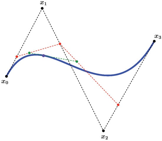
Figure 1. Illustration of the de Casteljau algorithm. Cubic polynomial in blue.

The curve $[0,1]\ni t\mapsto {\beta }_3\left(t\right):={\beta }_3(t,x_0,x_1,x_2,x_3)$ obtained in Algorithm 1 is called cubic polynomial in M, and in Figure 1 it is represented by the blue curve. It is important to observe that this curve joins the points $x_0$ (at $t=0$) and $x_3$ (at $t=1$), but does not pass through the other two points $x_1$ and $x_2$. The latter are called control points, since they influence the shape of the curve.

Algorithm 1 Generalized de Casteljau algorithm

Given four distinct points $x_0$, $x_1$, $x_2$ and $x_3$ in M:  Step 1  Construct three geodesic arcs, ${\beta }_1(t,x_i,x_{i+1})$, $i=0,1,2$, joining $x_i$ to $x_{i+1}$. In the illustration, these geodesic arcs are represented by the black dotted lines.  Step 2  For every $t\in [0,1]$, construct two geodesic arcs $${\beta }_2(s,x_i,x_{i+1},x_{i+2})={\beta }_1(s,{\beta }_1(t,x_i,x_{i+1}),{\beta }_1(t,x_{i+1},x_{i+2}))$$ for $i=0,1$, joining ${\beta }_1(t,x_i,x_{i+1})$ to ${\beta }_1(t,x_{i+1},x_{i+2})$. In the illustration, these geodesic arcs are represented by the red dotted lines.  Step 3  For every $t\in [0,1]$, construct the geodesic arc $${\beta }_3(s,x_0,x_1,x_2,x_3)={\beta }_1(s,{\beta }_2(t,x_0,x_1,x_2),{\beta }_2(t,x_1,x_2,x_3)),$$ joining ${\beta }_2(t,x_0,x_1,x_2)$ to ${\beta }_2(t,x_1,x_2,x_3)$. In the illustration, this geodesic arc is represented by the green dotted line. The dark blue dot represents the point in ${\beta }_3(s,x_0,x_1,x_2,x_3)$ corresponding to $s=t$.

Since the basic ingredients used in the de Casteljau algorithm are geodesic arcs, Riemannian geometry provides enough tools to formulate this construction theoretically. However, often those simple curves are implicitly defined by a set of nonlinear differential equations, so Algorithm 1 can be practically implemented only when the calculation of the geodesic arcs can be reduced to a manageable form.

This algorithm can be generalized to generate polynomials of any degree and also to generate ${\mathcal{C}}^2$-smooth cubic polynomial splines by piecing together, in a sufficiently smooth manner, several cubic polynomials. These curves are particularly useful in many engineering applications.

8.1.1. Cubic Polynomials in Graßmannians

Cubic polynomial curves on ${\mathbf{Gr}}_{n,k}^{\mathrm{proj}}$ were derived in [30], using the generalized de Casteljau algorithm above. The next result contains the explicit formula for such curves. We call attention to the meaning of the superscripts in the operators ${\Omega }_i^j$ that appear in the next proposition. Those superscripts have been chosen to agree with the step number of the algorithm where they are defined, and that will become clear in Remark 12.

Proposition 2. 

Given four distinct points $P_i$, for $i=0,1,2,3$, in ${\mathbf{Gr}}_{n,k}^{\mathrm{proj}}$, the curve

$$\begin{array}{cc}\hfill t\in [0,1]\mapsto {\beta }_3\left(t\right)& ={\mathrm{e}}^{t{\Omega }_0^3\left(t\right)}{\mathrm{e}}^{t{\Omega }_0^2\left(t\right)}{\mathrm{e}}^{t{\Omega }_0^1}{P}_0{\mathrm{e}}^{-t{\Omega }_0^1}{\mathrm{e}}^{-t{\Omega }_0^2\left(t\right)}{\mathrm{e}}^{-t{\Omega }_0^3\left(t\right)}\hfill \\ \hfill & ={\mathrm{e}}^{t{\mathrm{ad}}_{{\Omega }_0^3\left(t\right)}}{\mathrm{e}}^{t{\mathrm{ad}}_{{\Omega }_0^2\left(t\right)}}{\mathrm{e}}^{t{\mathrm{ad}}_{{\Omega }_0^1}}{P}_0,\hfill \end{array}$$

(95)

where, for $i=0,1,2$ and $j=2,3$,

$${\mathrm{e}}^{2{\Omega }_i^1}=(I-2P_{i+1})(I-2P_i),{\mathrm{e}}^{2{\Omega }_i^j\left(t\right)}={\mathrm{e}}^{2t{\Omega }_{i+1}^{j-1}\left(t\right)}{\mathrm{e}}^{2(1-t){\Omega }_i^{j-1}\left(t\right)},$$

(96)

is the cubic polynomial in ${\mathbf{Gr}}_{n,k}^{\mathrm{proj}}$, obtained by the generalized de Casteljau algorithm associated to the points $P_i$, with $i=0,1,2,3$. Moreover, for every $t\in [0,1]$,

$${\Omega }_i^1{P}_i+P_i{\Omega }_i^1={\Omega }_i^1,i=0,1,2,$$

(97)

$${\Omega }_i^2\left(t\right)\left({\mathrm{e}}^{t{\Omega }_i^1}{P}_0{\mathrm{e}}^{-t{\Omega }_i^1}\right)+\left({\mathrm{e}}^{t{\Omega }_i^1}{P}_0{\mathrm{e}}^{-t{\Omega }_i^1}\right){\Omega }_i^2\left(t\right)={\Omega }_i^2\left(t\right),i=0,1,$$

(98)

$${\Omega }_0^3\left(t\right)\left({\mathrm{e}}^{t{\Omega }_0^2\left(t\right)}{\mathrm{e}}^{t{\Omega }_0^1}{P}_0{\mathrm{e}}^{-t{\Omega }_0^1}{\mathrm{e}}^{-t{\Omega }_0^2\left(t\right)}\right)+\left({\mathrm{e}}^{t{\Omega }_0^2\left(t\right)}{\mathrm{e}}^{t{\Omega }_0^1}{P}_0{\mathrm{e}}^{-t{\Omega }_0^1}{\mathrm{e}}^{-t{\Omega }_0^2\left(t\right)}\right){\Omega }_0^3\left(t\right)={\Omega }_0^3\left(t\right).$$

(99)

Proof. 

See [30]. □

Remark 12. 

We briefly explain how Algorithm 1 generates the curve (95), subject to (96) and (97). For that, we use formula (34) for the geodesic arc that joins two given points, and identity (14).

In Step 1, the geodesic arc joining $P_i$ to $P_{i+1}$ is given by ${\beta }_1(t,P_i,P_{i+1})={\mathrm{e}}^{t{\Omega }_i^1}{P}_i{\mathrm{e}}^{-t{\Omega }_i^1}$, where ${\mathrm{e}}^{2{\Omega }_i^1}=(I-2P_{i+1})(I-2P_i)$. Taking into account identity (14), it is clear that the first condition in (97) holds.

In Step 2, we obtain ${\beta }_2(s,P_0,P_1,P_2)={\mathrm{e}}^{s{\Omega }_0^2\left(t\right)}{\beta }_1(t,P_0,P_1){\mathrm{e}}^{-s{\Omega }_0^2\left(t\right)},$ with

$${\mathrm{e}}^{2{\Omega }_0^2\left(t\right)}=(I-2{\beta }_1(t,P_1,P_2))(I-2{\beta }_1(t,P_0,P_1)).$$

(100)

Replace in (100), $P_1$ by ${\mathrm{e}}^{{\Omega }_0^1}{P}_0{\mathrm{e}}^{-{\Omega }_0^1}$, ${\beta }_1(t,P_i,P_{i+1})$ by its expression above, using (14), we get

$$\begin{array}{cc}\hfill {\mathrm{e}}^{2{\Omega }_0^2\left(t\right)}& =(I-2{\mathrm{e}}^{t{\Omega }_1^1}{\mathrm{e}}^{{\Omega }_0^1}{P}_0{\mathrm{e}}^{-{\Omega }_0^1}{\mathrm{e}}^{-t{\Omega }_1^1})(I-2{\mathrm{e}}^{t{\Omega }_0^1}{P}_0{\mathrm{e}}^{-t{\Omega }_0^1})\hfill \\ \hfill & ={\mathrm{e}}^{t{\Omega }_1^1}{\mathrm{e}}^{{\Omega }_0^1}(I-2P_0){\mathrm{e}}^{-{\Omega }_0^1}{\mathrm{e}}^{-t{\Omega }_1^1}{\mathrm{e}}^{t{\Omega }_0^1}(I-2P_0){\mathrm{e}}^{-t{\Omega }_0^1}\hfill \\ \hfill & ={\mathrm{e}}^{2t{\Omega }_1^1}{\mathrm{e}}^{2{\Omega }_0^1}(I-2P_0)(I-2P_0){\mathrm{e}}^{-2t{\Omega }_0^1}\hfill \\ \hfill & ={\mathrm{e}}^{2t{\Omega }_1^1}{\mathrm{e}}^{2(1-t){\Omega }_0^1},\hfill \end{array}$$

(101)

which is the second expression in (96) for $(i,j)=(0,2)$.

Moreover, the equality in the first line of (101) and (14) enables to conclude that the second condition in (97) holds for $i=0$.

Similar arguments can be used to obtain the other geodesic arc in Step 2 and the one in Step 3, together with the corresponding constraints in (97).

For the sake of completeness, we also include here the relationship between the control points $P_1$ and $P_2$ and the initial and final velocities of the curve (95), see [30].

The cubic polynomial ${\beta }_3$ that satisfies the boundary conditions

$${\beta }_3\left(0\right)=P_0,{\beta }_3\left(1\right)=P_3,{\dot{\beta }}_3\left(0\right)=[W_0,P_0],{\dot{\beta }}_3\left(1\right)=[W_3,P_3],$$

(102)

with $W_i=-W_i^{\top }$, for $i=1,3$, satisfying $W_i{P}_i+P_i{W}_i=W_i$, is generated by the de Casteljau algorithm associated to the points $P_i,i=0,1,2,3$, where the controls points are given in terms of the boundary data (102) as:

$$\begin{array}{cc}\hfill P_1& =\frac{1}{2}\left(I-{\mathrm{e}}^{\frac{2}{3}{W}_0}(I-2P_0)\right),\hfill \\ \hfill P_2& =\frac{1}{2}\left(I-{\mathrm{e}}^{-\frac{2}{3}{W}_3}(I-2P_3)\right).\hfill \end{array}$$

(103)

Remark 13. 

Although the formulas in Proposition 2 appear to be relatively manageable, they are not appropriate for the implementation of the algorithm due to their computational cost. It is exactly to overcome this burden that the formulas derived in Section 5.1 can be extremely useful.

8.1.2. Orthogonal Cubic Polynomials

Here, we present the cubic polynomials generated by the de Casteljau algorithm when $M={\mathbf{O}}_n$. This follows immediately from the work in [7], which was dedicated to connected and compact Lie groups and to spheres. The only difference here is that we have to assume that the initial data (the given four points) lives in one of the two connected components of the orthogonal group, in which case the resulting cubic stays in that component. Here, we use capital greek letters for points in ${\mathbf{O}}_n$, capital Roman letters for elements in its Lie algebra and, for convenience, denote the curves in the de Casteljau algorithm by $p_i$ instead of ${\beta }_i$. As in the Graßmannian case, the superscripts in the operators $V_i^j$ that appear in the next proposition have been chosen to agree with the step number of the algorithm where they are defined. This will become clear in Remark 14.

Proposition 3. 

Given four distinct points ${\theta }_i$, $i=0,1,2,3$, in one of the two connected components of ${\mathbf{O}}_n$, the curve defined by

$$p_3\left(t\right)={\mathrm{e}}^{t{V}_0^3\left(t\right)}{\mathrm{e}}^{t{V}_0^2\left(t\right)}{\mathrm{e}}^{t{V}_0^1}{\theta }_0,$$

(104)

where $V_i^1$, for $i=0,1,2$, is the infinitesimal generator of the geodesic arc joining the point ${\theta }_i$ (at $t=0$) to ${\theta }_{i+1}$ (at $t=1$), that is, ${\theta }_{i+1}={\mathrm{e}}^{V_i^1}{\theta }_i$, and for every $t\in [0,1]$ the Lie algebra elements $V_i^j$ are defined by:

$${\mathrm{e}}^{V_i^j\left(t\right)}={\mathrm{e}}^{t{V}_{i+1}^{j-1}\left(t\right)}{\mathrm{e}}^{(1-t)V_i^{j-1}\left(t\right)},\mathrm{for}j=2,3,$$

(105)

is the cubic polynomial in ${\mathbf{O}}_n$ generated by the de Casteljau algorithm, associated to ${\theta }_0,{\theta }_1,{\theta }_2$ and ${\theta }_3$.

Proof. 

See [7]. □

Remark 14. 

To check that Algorithm 1 generates the curve (104), subject to (105), it is enough to look at the expressions for the curves obtained in each of the three steps, taking into consideration the formula for geodesic arcs that join two given points in the orthogonal group.

In Step 1, the geodesic arc joining ${\theta }_i$ to ${\theta }_{i+1}$ is given by $p_1(t,{\theta }_i,{\theta }_{i+1})={\mathrm{e}}^{t{V}_i^1}{\theta }_i$, where ${\mathrm{e}}^{V_i^1}={\theta }_{i+1}{\theta }_i^{-1}$.

In Step 2, we obtain $p_2(s,{\theta }_0,{\theta }_1,{\theta }_2)={\mathrm{e}}^{s{V}_0^2\left(t\right)}{\mathrm{e}}^{t{V}_0^1}{\theta }_0,$ with ${\mathrm{e}}^{V_0^2\left(t\right)}{\mathrm{e}}^{t{V}_0^1}{\theta }_0={\mathrm{e}}^{t{V}_1^1}{\theta }_1$. However, the last identity is equivalent to ${\mathrm{e}}^{V_0^2\left(t\right)}{\mathrm{e}}^{t{V}_0^1}{\theta }_0={\mathrm{e}}^{t{V}_1^1}{\mathrm{e}}^{V_0^1}{\theta }_0$, or to ${\mathrm{e}}^{V_0^2\left(t\right)}={\mathrm{e}}^{t{V}_1^1}{\mathrm{e}}^{(1-t)V_0^1}.$

Similarly, the second geodesic arc is $p_2(s,{\theta }_1,{\theta }_2,{\theta }_3)={\mathrm{e}}^{s{V}_1^2\left(t\right)}{\mathrm{e}}^{t{V}_1^1}{\theta }_1$, with ${\mathrm{e}}^{V_1^2\left(t\right)}={\mathrm{e}}^{t{V}_2^1}{\mathrm{e}}^{(1-t)V_1^1}.$

In Step 3, $p_3(s,{\theta }_0,{\theta }_1,{\theta }_2,{\theta }_3)={\mathrm{e}}^{s{V}_0^3\left(t\right)}{\mathrm{e}}^{t{V}_0^2\left(t\right)}{\mathrm{e}}^{t{V}_0^1}{\theta }_0$, with ${\mathrm{e}}^{V_0^3\left(t\right)}{\mathrm{e}}^{t{V}_0^2\left(t\right)}{\mathrm{e}}^{t{V}_0^1}{\theta }_0$ =${\mathrm{e}}^{t{V}_1^2\left(t\right)}{\mathrm{e}}^{t{V}_1^1}{\theta }_1$.

Taking into consideration that ${\theta }_1={\mathrm{e}}^{V_0^1}{\theta }_0$ and ${\mathrm{e}}^{V_0^2\left(t\right)}={\mathrm{e}}^{t{V}_1^1}{\mathrm{e}}^{(1-t)V_0^1}$, it simplifies to ${\mathrm{e}}^{V_0^3\left(t\right)}={\mathrm{e}}^{t{V}_1^2\left(t\right)}{\mathrm{e}}^{(1-t)V_0^2\left(t\right)}$.

The relationship between the control points ${\theta }_1$ and ${\theta }_2$ and the initial and final velocities of the curve (104) follows immediately from Theorem 2.5 in [7], which states that

$${\dot{p}}_3\left(0\right)=3V_0^1{\theta }_0,{\dot{p}}_3\left(1\right)=3V_2^1{\theta }_3.$$

(106)

Indeed, the cubic polynomial $p_3$ that satisfies the boundary conditions

$$p_3\left(0\right)={\theta }_0,p_3\left(1\right)={\theta }_3,{\dot{p}}_3\left(0\right)=W_0{\theta }_0,{\dot{p}}_3\left(1\right)=W_3{\theta }_3,$$

(107)

can be generated by the de Casteljau algorithm with controls points

$${\theta }_1={\mathrm{e}}^{W_0/3}{\theta }_0,{\theta }_2={\mathrm{e}}^{-W_3/3}{\theta }_3.$$

(108)

8.1.3. Comparing Cubic Polynomials in ${\mathbf{O}}_n$ with Cubic Polynomials in Graßmannians

We take advantage of the fact that ${\mathbf{Gr}}_{n,k}^{\mathrm{refl}}=I-2{\mathbf{Gr}}_{n,k}^{\mathrm{proj}}$ lives in ${\mathbf{O}}_n$ to compare the cubic polynomial in Proposition 2 with the orthogonal cubic polynomial in Proposition 3.

Theorem 4. 

Let ${\beta }_3\left(t\right)$ be the cubic polynomial in ${\mathbf{Gr}}_{n,k}^{\mathrm{proj}}$ associated to the points $P_i$, $i=0,1,2,3$, given in Proposition 2, and $p_3\left(t\right)$ the cubic polynomial in ${\mathbf{O}}_n$ associated to the points ${\theta }_i=I-2P_i$, given in Proposition 3. Then,

$$p_3\left(t\right)=I-2{\beta }_3\left(t\right).$$

(109)

Proof. 

First we show that when ${\theta }_i=I-2P_i$, we have $V_i^j=2{\Omega }_i^j$, where the $V_i^j$ are as defined in Proposition 3 and the ${\Omega }_i^j$ as defined in Proposition 2. Indeed,

$${\theta }_{i+1}={\mathrm{e}}^{V_i^1}{\theta }_i⟺(I-2P_{i+1})(I-2P_i)={\mathrm{e}}^{V_i^1},$$

(110)

and comparing with the first identity in (96) we conclude that $V_i^1=2{\Omega }_i^1$, $i=0,1,2$. Using these relationships and the second identity in (96), we can write

$${\mathrm{e}}^{V_i^2\left(t\right)}={\mathrm{e}}^{t{V}_{i+1}^1}{\mathrm{e}}^{(1-t)V_i^1}={\mathrm{e}}^{2t{\Omega }_{i+1}^1}{\mathrm{e}}^{2(1-t){\Omega }_i^1}={\mathrm{e}}^{2{\Omega }_i^2\left(t\right)}.$$

(111)

So, $V_i^2=2{\Omega }_i^2$, for $i=0,1$. Similarly, using these relations and the second identity in (96), with $(i,j)=(0,3)$, we conclude that $V_0^3=2{\Omega }_0^3$. So, since

$${\beta }_3\left(t\right)={\mathrm{e}}^{t{\Omega }_0^3\left(t\right)}{\mathrm{e}}^{t{\Omega }_0^2\left(t\right)}{\mathrm{e}}^{t{\Omega }_0^1}{P}_0{\mathrm{e}}^{-t{\Omega }_0^1}{\mathrm{e}}^{-t{\Omega }_0^2\left(t\right)}{\mathrm{e}}^{-t{\Omega }_0^3\left(t\right)}$$

(112)

satisfies all the constraints in Proposition 2, also

$$p_3\left(t\right)={\mathrm{e}}^{2t{\Omega }_0^3\left(t\right)}{\mathrm{e}}^{2t{\Omega }_0^2\left(t\right)}{\mathrm{e}}^{2t{\Omega }_0^1}{\theta }_0,$$

(113)

satisfies all the constraints in Proposition 3.

Finally, we prove the relationship between ${\beta }_3\left(t\right)$ and $p_3\left(t\right)$, systematically using the result in Lemma 1 and the constraints (97). Indeed,

$$\begin{array}{cc}\hfill I-2{\beta }_3\left(t\right)& ={\mathrm{e}}^{t{\Omega }_0^3\left(t\right)}\left(I-2{\mathrm{e}}^{t{\Omega }_0^2\left(t\right)}{\mathrm{e}}^{t{\Omega }_0^1}{P}_0{\mathrm{e}}^{-t{\Omega }_0^1}{\mathrm{e}}^{-t{\Omega }_0^2\left(t\right)}\right){\mathrm{e}}^{-t{\Omega }_0^3\left(t\right)}\hfill \\ \hfill & ={\mathrm{e}}^{2t{\Omega }_0^3\left(t\right)}{\mathrm{e}}^{t{\Omega }_0^2\left(t\right)}\left(I-2{\mathrm{e}}^{t{\Omega }_0^1}{P}_0{\mathrm{e}}^{-t{\Omega }_0^1}\right){\mathrm{e}}^{-t{\Omega }_0^2\left(t\right)}\hfill \\ \hfill & ={\mathrm{e}}^{2t{\Omega }_0^3\left(t\right)}{\mathrm{e}}^{2t{\Omega }_0^2\left(t\right)}\left(I-2{\mathrm{e}}^{t{\Omega }_0^1}{P}_0{\mathrm{e}}^{-t{\Omega }_0^1}\right)\hfill \\ \hfill & ={\mathrm{e}}^{2t{\Omega }_0^3\left(t\right)}{\mathrm{e}}^{2t{\Omega }_0^2\left(t\right)}{\mathrm{e}}^{2t{\Omega }_0^1}\left(I-2P_0\right)={\mathrm{e}}^{2t{\Omega }_0^3\left(t\right)}{\mathrm{e}}^{2t{\Omega }_0^2\left(t\right)}{\mathrm{e}}^{2t{\Omega }_0^1}{\theta }_0\hfill \\ \hfill & =p_3\left(t\right).\hfill \end{array}$$

(114)

□

Remark 15. 

Since ${\mathbf{Gr}}_{n,k}^{\mathrm{refl}}$ is a submanifold of ${\mathbf{O}}_n$, the last result tells us that if ${\theta }_i\in {\mathbf{O}}_n\cap {\mathbf{Gr}}_{n,k}^{\mathrm{refl}}$ holds for all data points, the whole de Casteljau construction in ${\mathbf{O}}_n$ actually takes place inside ${\mathbf{Gr}}_{n,k}^{\mathrm{refl}}$. This observation is due to two important facts. First of all, the de Casteljau algorithm is solely based on recursive geodesic interpolation. Secondly, ${\mathbf{Gr}}_{n,k}^{\mathrm{refl}}$ is a totally geodesic submanifold of ${\mathbf{O}}_n$, since any geodesic in ${\mathbf{Gr}}_{n,k}^{\mathrm{refl}}$ is a geodesic in ${\mathbf{O}}_n$. Indeed, every geodesic in ${\mathbf{Gr}}_{n,k}^{\mathrm{refl}}$ that starts at a point $I_n-2P$, $P\in {\mathbf{Gr}}_{n,k}^{\mathrm{proj}}$, is of the form $\gamma \left(t\right)={\mathrm{e}}^{t\Omega }(I-2P){\mathrm{e}}^{-t\Omega }$, with $\Omega \in {\mathfrak{so}}_n$ satisfying $\Omega P+P\Omega =\Omega$. However, due to the second identity in Lemma 1, $\gamma \left(t\right)={\mathrm{e}}^{2t\Omega }(I-2P)$, which is a geodesic in ${\mathbf{O}}_n$.

9. Conclusions

In this work we have considered the so-called endpoint geodesic problem on Graßmannians. We presented explicit and closed fromulas for connecting two nonconjugate points on the real Graßmannian by a unique minimizing geodesic. The approach goes beyond earlier work as matrix exponentials and logarithms can be avoided. The special cases of projective spaces and unit spheres were handled as well. These results were applied to the important interpolation problem of implementing the de Casteljau algorithm on Graßmannians via iterated geodesic interpolation.

References

- Noakes, L.; Heinzinger, G.; Paden, B. Cubic splines on curved spaces. IMA J. Math. Control Inf. 1989, 6, 465–473. [Google Scholar] [CrossRef]
- Crouch, P.; Silva Leite, F. The dynamic interpolation problem: On Riemannian manifolds, Lie groups, and symmetric spaces. J. Dyn. Control Syst. 1995, 1, 177–202. [Google Scholar] [CrossRef]
- Camarinha, M.; Silva Leite, F.; Crouch, P. On the geometry of Riemannian cubic polynomials. Differ. Geom. Its Appl. 2001, 15, 107–135. [Google Scholar] [CrossRef]
- Popiel, T.; Noakes, L. Bézier curves and C2 interpolation in Riemannian manifolds. J. Approx. Theory 2007, 148, 111–127. [Google Scholar] [CrossRef]
- De Casteljau, P. Outillages Méthodes Calcul. Technical Report—André Citroën Automobiles SA. 1959. [Google Scholar]
- Park, F.; Ravani, B. Bézier Curves on Riemannian Manifolds and Lie Groups with Kinematics Applications. ASME J. Mech. Des. 1995, 117, 36–40. [Google Scholar] [CrossRef]
- Crouch, P.; Kun, G.; Silva Leite, F. The De Casteljau algorithm on Lie groups and spheres. J. Dynam. Control Syst. 1999, 5, 397–429. [Google Scholar] [CrossRef]
- Zhang, E.; Noakes, L. Optimal interpolants on Grassmann manifolds. Optim. Interpolants Grassmann Manifolds. Math. Control Signals Syst. 2019, 31, 363–383. [Google Scholar] [CrossRef]
- Zhang, E.; Noakes, L. The cubic de Casteljau construction and Riemannian cubics. Comput. Aided Geom. Des. 2019, 75, 101789. [Google Scholar] [CrossRef]
- Alashkar, T.; Ben Amor, B.; Daoudi, M.; Berretti, S. A Grassmann framework for 4D facial shape analysis. Pattern Recognit. 2016, 57, 21–30. [Google Scholar] [CrossRef]
- Shi, X.; Styner, M.; Lieberman, J.; Ibrahim, J.G.; Lin, W.; Zhu, H. Intrinsic Regression Models for Manifold-Valued Data. In Proceedings of the Medical Image Computing and Computer-Assisted Intervention (MICCAI), London, UK, 20–24 September 2009; Yang, G., Hawkes, D., Rueckert, D., Noble, A., Taylor, C., Eds.; Springer: Berlin/Heidelberg, Germany, 2009; Volume 5762, pp. 192–199. [Google Scholar]
- Batzies, E.; Hüper, K.; Machado, L.; Silva Leite, F. Geometric Mean and Geodesic Regression on Grassmannians. Linear Algebra Its Appl. 2015, 466, 83–101. [Google Scholar] [CrossRef]
- Eschenburg, J.H. Lecture Notes on Symmetric Spaces. Available online: https://myweb.rz.uni-augsburg.de/~eschenbu/symspace.pdf (accessed on 11 August 2023 ).
- Ziller, W. Lie Groups. Representation Theory and Symmetric Spaces. Available online: https://www2.math.upenn.edu/~wziller/math650/LieGroupsReps.pdf (accessed on 11 August 2023 ).
- O’Neill, B. Semi-Riemannian Geometry with Applications to Relativity; Academic Press, Inc.: New York, NY, USA, 1983. [Google Scholar]
- Gallier, J.; Quaintance, J. Differential Geometry and Lie Groups. A Computational Perspective; Springer: Cham, Switzerland, 2020. [Google Scholar]
- Loos, O. Symmetric Spaces. II: Compact Spaces and Classification; W. A. Benjamin, Inc.: New York, NY, USA; Amsterdam, The Netherlands, 1969. [Google Scholar]
- Loos, O. Symmetric Spaces. I: General Theory; W. A. Benjamin, Inc.: New York, NY, USA; Amsterdam, The Netherlands, 1969. [Google Scholar]
- Onishchik, A.L. Topology of Transitive Transformation Groups; Johann Ambrosius Barth: Leipzig, Germany, 1994. [Google Scholar]
- Helmke, U.; Hüper, K.; Trumpf, J. Newton’s Method on Graßmann Manifolds. arXiv 2007, arXiv:0709.2205. [Google Scholar]
- Lee, J.M. Introduction to Riemannian Manifolds, 2nd ed.; Springer: Cham, Switzerland, 2018. [Google Scholar]
- Bendokat, T.; Zimmermann, R.; Absil, P.A. A Grassmann Manifold Handbook: Basic Geometry and Computational Aspects. arXiv 2020, arXiv:2011.13699. [Google Scholar]
- Stegemeyer, M. Endpoint Geodesics in Symmetric Spaces. Master’s Thesis, Institut für Mathematik, Julius-Maximilians-Universität Würzburg, Würzburg, Germany, 2020. [Google Scholar]
- Stewart, G. Matrix Algorithms. Vol. 1: Basic Decompositions; Society for Industrial and Applied Mathematics (SIAM): Philadelphia, PA, USA, 1998. [Google Scholar]
- Kobayashi, S.; Nomizu, K. Foundations of Differential Geometry; John Wiley & Sons, Inc.: New York, NY, USA, 1996; Volume 2. [Google Scholar]
- Kobayashi, S. Isometric imbeddings of compact symmetric spaces. Tôhoku Math. J. 1968, 20, 21–25. [Google Scholar] [CrossRef]
- Bertram, W. The Geometry of Jordan and Lie Structures; Springer: Berlin/Heidelberg, Germany, 2000. [Google Scholar]
- Bézier, P. The Mathematical Basis of the UNISURF CAD System; Butterworths: London, UK, 1986. [Google Scholar]
- Farin, G.; Hansford, D. The Essentials of CAGD; CRC Press: Boca Raton, FL, USA, 2000. [Google Scholar]
- Pina, F. Interpolation in the Generalized Essential Manifold. Ph.D. Thesis, Department of Mathematics, University of Coimbra, Coimbra, Portugal, 2020. [Google Scholar]
Disclaimer/Publisher’s Note: The statements, opinions and data contained in all publications are solely those of the individual author(s) and contributor(s) and not of MDPI and/or the editor(s). MDPI and/or the editor(s) disclaim responsibility for any injury to people or property resulting from any ideas, methods, instructions or products referred to in the content. |
© 2023 by the authors. Licensee MDPI, Basel, Switzerland. This article is an open access article distributed under the terms and conditions of the Creative Commons Attribution (CC BY) license (https://creativecommons.org/licenses/by/4.0/).