An Approach to Solving Direct and Inverse Scattering Problems for Non-Selfadjoint Schrödinger Operators on a Half-Line

Abstract

In this paper, an approach to solving direct and inverse scattering problems on the half-line for a one-dimensional Schrödinger equation with a complex-valued potential that is exponentially decreasing at infinity is developed. It is based on a power series representation of the Jost solution in a unit disk of a complex variable related to the spectral parameter by a Möbius transformation. This representation leads to an efficient method of solving the corresponding direct scattering problem for a given potential, while the solution to the inverse problem is reduced to the computation of the first coefficient of the power series from a system of linear algebraic equations. The approach to solving these direct and inverse scattering problems is illustrated by several explicit examples and numerical testing.

1. Introduction

Consider the one-dimensional Schrödinger equation

$$l\left[y\right]:=-y^{″}+q\left(x\right)y=\lambda y,x\in (0,\infty ),$$

(1)

with $\lambda \in \mathbb{C}$ and a complex-valued potential $q\left(x\right)$ satisfying the condition

$${\int }_0^{\infty }{e}^{\epsilon x}\left|q\left(x\right)\right|dx<\infty$$

(2)

for some $\epsilon >0$. By ρ, we denote the square root of $\lambda$ such that $\rho \in \overline{{\mathbb{C}}^{+}}:=\left\{w\in \mathbb{C}:Im\left(w\right)\ge 0\right\}$. In the present work, an approach to solving direct and inverse scattering problems for (1) under Condition (2) is developed.

Complex-valued potentials arise when studying parity time (PT)-symmetric potentials [1] (Chapter 1), [2], quasi-exactly solvable (QES) potentials [3,4], hydrodynamics, and magnetohydrodynamics [5]; see also [6,7,8].

Studying a Zakharov–Shabat system, even with a real-valued potential, naturally leads to a couple of equations of the form (1) with complex-valued potentials; see [9]. Indeed, consider the Zakharov–Shabat system

$${\overrightarrow{\upsilon }}_x\left(x\right)={\left(\begin{array}{c}{v}_1\left(x\right)\\ v_2\left(x\right)\end{array}\right)}_x=\left(\begin{array}{cc}-i\rho & u\left(x\right)\\ -u\left(x\right)& i\rho \end{array}\right)\overrightarrow{\upsilon }\left(x\right),0<x<\infty$$

(3)

where ρ is a complex spectral parameter and $u\left(x\right)$ is a real-valued potential.

The further transformation of $\overrightarrow{\upsilon }\left(x\right)$ is as follows:

$$\begin{array}{cc}\hfill y_1\left(x\right)& =v_2\left(x\right)-i{v}_1\left(x\right),\hfill \\ \hfill y_2\left(x\right)& =v_2\left(x\right)+i{v}_1\left(x\right)\hfill \end{array}$$

This leads to a pair of Schrödinger equations with complex-valued potentials

$$\begin{array}{cc}\hfill -y_1^{{}_{{}^{″}}}\left(x\right)+(-i{u}^{{}_{{}^{\prime }}}\left(x\right)-u^2\left(x\right))y_1\left(x\right)& ={\rho }^2{y}_1\left(x\right),\hfill \end{array}$$

(4)

$$\begin{array}{cc}\hfill -y_2^{{}_{{}^{″}}}\left(x\right)+(i{u}^{{}_{{}^{\prime }}}\left(x\right)-u^2\left(x\right))y_2\left(x\right)& ={\rho }^2{y}_2\left(x\right).\hfill \end{array}$$

(5)

Thus, the results of the present work are applicable to direct and inverse scattering problems for a Zakharov–Shabat system.

A direct scattering problem for (1) with a complex-valued potential was studied in a number of publications ([10,11,12,13]). Equation (1) under Condition (2) was considered in [12] (p. 292), [14,15,16,17,18,19,20] (p. 353), and [21,22].

It is well-known (see, e.g., [12] (p. 443), [18]) that (1) admits a unique solution, which we denote by $e(\rho ,x)$, satisfying the asymptotic equality

$$e(\rho ,x)=e^{i\rho x}(1+o\left(1\right)),x\to \infty .$$

This solution is called the Jost solution of (1). It admits the Levin integral representation [12] (see also [18,23,24])

$$e(\rho ,x)=e^{i\rho x}+{\int }_x^{\infty }A(x,t)e^{i\rho t}dt,Im\rho >-\frac{\epsilon }{2},x\ge 0$$

(6)

where for every fixed x, the kernel $A(x,t)$ belongs to ${\mathcal{L}}_2(x,\infty )$. In [25] (see also [26]) a Fourier–Laguerre series representation for $A(x,t)$ was proposed in the form

$$A(x,t)=\sum _{n=0}^{\infty }{a}_n\left(x\right)L_n(t-x)e^{\frac{x-t}{2}},$$

(7)

where $L_n\left(\tau \right)$ stands for the Laguerre polynomial of order n. A recurrent integration procedure was developed in [27] to calculate the coefficients $a_n\left(x\right)$. The substitution of (7) into (6) was found to lead to a series representation for the Jost solution [25,26]

$$\begin{array}{cc}\hfill e\left(\rho ,x\right)& =e^{i\rho x}\left(1+(z+1)\sum _{n=0}^{\infty }{(-1)}^n{z}^n{a}_n\left(x\right)\right),x\ge 0,\rho \in \overline{{\mathbb{C}}^{+}}\hfill \end{array}$$

(8)

where

$$z=z\left(\rho \right)=\frac{\left(\frac{1}{2}+i\rho \right)}{\left(\frac{1}{2}-i\rho \right)}·$$

(9)

In the present work, we consider the direct and inverse scattering problems for (1) subject to the homogeneous Dirichlet condition

$$y\left(0\right)=0,$$

(10)

however, the approach developed here is also applicable in the case of other boundary conditions, such as

$$y^{{}_{{}^{\prime }}}\left(0\right)-hy\left(0\right)=0$$

with $h\in \mathbb{C}$.

The problem (1) and (10) under Condition (2) possesses a continuous spectrum coinciding with the positive semi-axis $\lambda >0$, and may have a point spectrum that coincides with the squares of the non-real roots of the Jost function

$$e\left(\rho \right):=e(\rho ,0),$$

if such roots exist. Let us denote them as ${\rho }_1,\dots ,{\rho }_{\alpha }.$ Their multiplicity may be greater than one. In this case, instead of norming constants associated to the eigenvalues, the corresponding normalization polynomials $X_k\left(x\right)$ naturally arise (see Section 3.3 below).

As a component of the scattering data for (1), the scattering function

$$s\left(\rho \right):=\frac{e(-\rho )}{e\left(\rho \right)}$$

is considered in the strip $\left|Im\left(\rho \right)\right|<{\epsilon }_0$ where ${\epsilon }_0$ is sufficiently small (see Section 3.2 below).

The direct scattering problem for (1) and (10) consists of obtaining the set of the scattering data

$$\left\{{\left\{{\rho }_k,m_k,X_k\left(x\right)\right\}}_{k=1}^{\alpha },s\left(\rho \right)\right\}.$$

(11)

The overall approach developed in the present work to solve this problem is based on the representation (8). Indeed, the calculation of ${\left\{{\rho }_k\right\}}_{k=1}^{\alpha }$ is easily realizable with the aid of the argument principle theorem applied to find zeros of (8) in the unit disc. To the best of our knowledge, there has been no practical way of calculating the normalization polynomials. We propose a simple procedure for computing their coefficients by solving a finite system of linear algebraic equations. For this, an auxiliary result for the derivatives $\frac{{\partial }^m}{\partial z^m}e(\rho \left(z\right),x)$ is obtained.

The calculation of the scattering function $s\left(p\right)$ requires an analytic extension of the Jost function $e\left(\rho \right)$ obtained from (8), onto the strip $-{\epsilon }_0<Im\left(\rho \right)<0$. We explore different possibilities for such an extension, including the Padé approximants (see [28,29]) and the power series analytic continuation [30] (p. 150), [31]. This results in an efficient numerical method for solving the direct scattering problem.

The inverse scattering problem consists of recovering the potential $q\left(x\right)$ from the set of the scattering data. A general theory of this inverse problem can be found in [12,13,20] (p. 353), [24,32,33,34,35]. Here, we use the representation (7) for the numerical solution of the problem, thus extending the approach developed in [25,26,36,37,38] to the non-selfadjoint situation. The inverse Sturm–Liouville problem is reduced to an infinite system of linear algebraic equations. The potential $q\left(x\right)$ is recovered from the first component of the solution vector, which coincides with $a_0\left(x\right)$ in (7).

The reduction to the infinite system of linear algebraic equations is based on the substitution of the series representation (7) for the kernel $A(x,t)$ into the Gelfand–Levitan equation (see [39]),

$$A(x,t)={\int }_x^{\infty }A(x,u)f(u+t)du+f(x+t),0\le x\le t<\infty ,$$

(12)

where the function f can be computed from the set of scattering data (11):

$$\begin{array}{cc}\hfill f\left(x\right)& :=\frac{1}{2\pi }{\int }_{-\infty +i\eta }^{{}^{\infty +i\eta }}(s\left(\rho \right)-1)e^{ix\rho }d\rho -\sum _{k=1}^{\alpha }{X}_k\left(x\right)e^{i{\rho }_{k}x},0<\eta <{\epsilon }_0.\hfill \end{array}$$

To approximate the complex-valued function $a_0\left(x\right)$, we consider the truncated system of linear algebraic equations, for which the existence, uniqueness and stability of the solution is proved.

Finally, we illustrate the proposed approach by numerical calculations performed in Matlab2021a.

We discuss the details of the numerical implementation of the method: its convergence, stability and accuracy. In a couple of examples, we show the “in-out” performance of the approach, i.e., we solve the direct problem numerically and use the results of our computation as the input data to solve the inverse problem.

The approach based on the representations (7) and (8) leads to efficient numerical methods for solving both direct and inverse scattering problems.

In Section 2, we recall the series representations for the kernel $A(x,t)$ and for the Jost solution, then prove additional results related to these representations. In Section 3, we recall the set of scattering data and put forward an algorithm for solving the direct scattering problem. Additionally, we present analytical examples. In Section 4, the approach for solving the inverse scattering problem is developed. Analytical examples from Section 2 are considered in order to illustrate the approach. In Section 5, we discuss the numerical implementation of the algorithms proposed for solving the direct and inverse scattering problems. Section 6 contains some concluding remarks.

2. Series Representations for the Transmutation Operator Kernel and Jost Solution

Consider the one-dimensional Schrödinger equation on the half-line (1) where $\lambda ={\rho }^2\in \mathbb{C}$ is the spectral parameter. The potential $q\left(x\right)$ is a complex-valued function satisfying Condition (2) for some $\epsilon >0$.

Equation (1) is considered on the class of functions $\mathcal{D}\left(l\right)=\left\{y\in {\mathcal{W}}^{2,2}(0,\infty ):l\left[y\right]\in {\mathcal{L}}_2(0,\infty )\right\}$.

Series Representation for Solutions of the One-Dimensional Schrödinger Equation

Equation (1) possesses the unique so-called Jost solution $e(\rho ,x)$ (see, e.g., [12] (p. 443), [18]), which for all $x\ge 0$ is a holomorphic function of $\rho$ in the half-plane $Im\rho \ge 0$ and satisfies the asymptotic relation

$$e(\rho ,x)=e^{i\rho x}(1+o\left(1\right))\mathrm{when}x\to \infty \mathrm{and}Im\rho \ge 0.$$

(13)

The function $e\left(\rho \right):=e(\rho ,0)$ is called the Jost function.

Remark 1. 

Under the assumption $q\left(x\right)\in \mathcal{L}(0,\infty )$ instead of (2), for every $x\ge 0$ the solution $e(\rho ,x)$ is continuous with respect to $\rho$ for $\rho \in \overline{{\mathbb{C}}^{+}}\setminus \left\{0\right\}$ and holomorphic with respect to $\rho$ for $\rho \in {\mathbb{C}}^{+}$. If in addition $(1+x)q\left(x\right)\in \mathcal{L}(0,\infty )$, the functions $e^{\left(\nu \right)}(\rho ,x)$, $\nu =0,1$ are continuous for $\rho \in \overline{{\mathbb{C}}^{+}},x\ge 0$ (see [24] (p. 105)).

Remark 2. 

Under Condition (2), the Jost solution satisfies the asymptotic relations

$$\frac{{\partial }^j}{\partial x^j}e(\rho ,x)={\left(ix\right)}^{\left(j\right)}{e}^{i\rho x}+o\left(e^{-\frac{\epsilon }{2}x}\right),j=0,1,\dots \mathit{when}x\to \infty ,$$

provided the existence of these derivatives; see [21].

The solution $e(\rho ,x)$ admits the Levin integral representation [12]

$$e(\rho ,x)=e^{ix\rho }+{\int }_x^{\infty }A(x,t)e^{i\rho t}dt,Im\rho \ge 0,x\ge 0,$$

(14)

where $A(x,t)$ is a complex-valued continuous function for $0\le x\le t<\infty$. Denote $Q\left(x\right):={∥q∥}_{\mathcal{L}(x,\infty )}$. The kernel $A(x,t)$ admits the bound [24] (p. 108)

$$\left|A(x,t)\right|\le \frac{1}{2}Q\left(\frac{x+t}{2}\right)exp\left({∥Q∥}_{\mathcal{L}(x,\infty )}-{∥Q∥}_{\mathcal{L}\left(\frac{x+t}{2},\infty \right)}\right).$$

(15)

Under Condition (2), the Jost solution is extensible onto the half-plane $Im\rho >-\frac{\epsilon }{2}$ through the Levin representation (14). The extension satisfies (13) for $Im\rho >-\frac{\epsilon }{2}$.

Proposition 1. 

Under Condition (2), the kernel $A(x,t)$ admits the bound

$$\left|A(x,t)\right|\le \frac{1}{2}{e}^{-\epsilon \left(\frac{x+t}{2}\right)}\left({\int }_{\frac{x+t}{2}}^{\infty }{e}^{\epsilon \tau }\left|q\left(\tau \right)\right|d\tau \right)exp\left(\frac{C_{\epsilon }}{\epsilon }\left(e^{-\epsilon x}-e^{-\epsilon \frac{x+t}{2}}\right)\right),0\le x\le t<\infty ,$$

(16)

where $C_{\epsilon }={\int }_0^{\infty }{e}^{\epsilon t}\left|q\left(t\right)\right|dt.$

Proof. 

Under Condition (2), the potential $q\left(x\right)$ satisfies the inequality

$$Q\left(x\right)\le e^{-\epsilon x}{\int }_x^{\infty }{e}^{\epsilon t}\left|q\left(t\right)\right|dt=C_{\epsilon }{e}^{-\epsilon x}.$$

(17)

Moreover, for any fixed $x\in [0,\infty )$ we have [12] (p. 317)

$${∥Q∥}_{\mathcal{L}(x,\infty )}\le \frac{C_{\epsilon }}{\epsilon }{e}^{-\epsilon x}.$$

(18)

Thus, substitution of (17) and (18) into (15) gives us (16). □

Additionally, the kernel $A(x,t)$ has first continuous derivatives that satisfy the inequalities [12] (p. 305)

$$\left|A_x(x,t)\right|,\left|A_t(x,t)\right|\le \frac{1}{4}\left|q\left(\frac{x+t}{2}\right)\right|+C_{\epsilon }exp\left(-\epsilon \left(\frac{3}{2}x+t\right)\right),$$

(19)

and the equality [12] (p. 328)

$$A(x,x)=\frac{1}{2}{\int }_x^{\infty }q\left(t\right)dt.$$

(20)

As was pointed out in [25], since $A(x,·)\in {\mathcal{L}}_2(x,\infty )$, the function

$$\begin{array}{cc}\hfill a(x,t)& :=e^{\frac{t}{2}}A(x,t+x)\hfill \end{array}$$

(21)

belongs to $L_2([0,\infty );e^{-t})$ and hence admits the series representation

$$a(x,t)=\sum _{n=0}^{\infty }{a}_n\left(x\right)L_n\left(t\right),$$

(22)

where $L_n\left(t\right)$ stands for the Laguerre polynomial of order n and $a_n\left(x\right)$ are complex-valued functions such that ${\left\{a_n\left(x\right)\right\}}_{n=0}^{\infty }\in l_2$ for any $x\ge 0$. For all $x\ge 0$, the series (22) converges in the norm of ${\mathcal{L}}_2([0,\infty );e^{-t})$. Thus,

$$A(x,t)=\sum _{n=0}^{\infty }{a}_n\left(x\right)L_n(t-x)e^{\frac{x-t}{2}}$$

(23)

and

$$\sum _{n=0}^{\infty }{a}_n\left(x\right)=A(x,x)=\frac{1}{2}{\int }_x^{\infty }q\left(t\right)dt.$$

(24)

This series representation was obtained in [25] for real-valued $q\left(x\right)$. However, (23) remains true in the non-selfadjoint case as well.

Proposition 2. 

For any fixed $x\ge 0$, the series

$$a(x,t)=\sum _{n=0}^{\infty }{a}_n\left(x\right)L_n\left(t\right),t\in [0,\infty )$$

(25)

converges pointwise.

Proof. 

We use [40] (Theorem 6.5), and thus need to verify that the following assertions are true.

1. $a(x,·)$ is of class $\mathcal{L}\left([0,\infty );e^{-t}\right)$.

2. $a(x,·)$ is $\gamma$-Hölder continuous, i.e., there exists $0<\gamma \le 1$, such that

$$\left|a\left(x,t_0\right)-a(x,t)\right|\le M{\left|t_0-t\right|}^{\gamma },$$

for some constant $M>0$ and arbitrary t, $t_0\in [0,\infty )$.

3. The integrals

$${\int }_0^1{t}^{-3/4}\left|a(x,t)\right|dt,{\int }_{{}_1}^{\infty }{e}^{-t/2}\left|a(x,t)\right|dt$$

(26)

exist.

To prove the first assertion, it is enough to consider estimate (15). Indeed,

$$\begin{array}{cc}\hfill {\int }_0^{\infty }{e}^{-t}\left|a(x,t)\right|dt& \le {\int }_0^{\infty }\left|A(x,x+t)\right|dt\hfill \\ \hfill & \le \frac{1}{2}{\int }_0^{\infty }Q\left(\frac{2x+t}{2}\right)exp\left({∥Q∥}_{\mathcal{L}(x,\infty )}-{∥Q∥}_{\mathcal{L}\left(\frac{2x+t}{2},\infty \right)}\right)dt\hfill \\ \hfill & \le \frac{exp\left({∥Q∥}_{\mathcal{L}(x,\infty )}\right)}{2}{\int }_0^{\infty }Q\left(\frac{2x+t}{2}\right)exp\left(-{∥Q∥}_{\mathcal{L}\left(\frac{2x+t}{2},\infty \right)}\right)dt\hfill \\ \hfill & =exp\left({∥Q∥}_{\mathcal{L}(x,\infty )}\right){\int }_x^{\infty }Q\left(\tau \right)exp\left(-{∥Q∥}_{\mathcal{L}\left(\tau ,\infty \right)}\right)d\tau .\hfill \end{array}$$

Note that $\frac{d}{d\tau }{∥Q∥}_{\mathcal{L}\left(\tau ,\infty \right)}=Q\left(\tau \right)$ and therefore

$${\int }_x^{\infty }Q\left(\tau \right)exp\left(-{∥Q∥}_{\mathcal{L}\left(\tau ,\infty \right)}\right)d\tau =1-exp\left(-{∥Q∥}_{\mathcal{L}\left(x,\infty \right)}\right).$$

(27)

Thus,

$${\int }_0^{\infty }{e}^{-t}\left|a(x,t)\right|dt\le exp\left({∥Q∥}_{\mathcal{L}\left(x,\infty \right)}\right)-1<\infty .$$

The second assertion follows from the inclusion $A(x,·)\in C{}^1(x,\infty )$.

The existence of the first integral in (26) follows from the continuity of $a(x,·)$. Finally, for the second integral we have

$$\begin{array}{cc}\hfill {\int }_{{}_1}^{\infty }{e}^{-t/2}\left|a(x,t)\right|dt& ={\int }_{{}_1}^{\infty }\left|A(x,x+t)\right|dt\le {\int }_0^{\infty }\left|A(x,x+t)\right|dt,\hfill \end{array}$$

and thus, from the proof of the first assertion, we obtain ${\int }_{{}_1}^{\infty }{e}^{-t/2}\left|a(x,t)\right|dt<\infty .$

Now, the application of Theorem 6.5 from [40] completes the proof. □

Following [25] (see also [26] (p. 63)), the substitution of (23) into (14) and termwise integration lead to the series representation (8) for the Jost solution.

The series (8) is convergent in the open unit disk of the complex z-plane, $\mathbb{D}:=\left\{z\in \mathbb{C}:\left|z\right|<1\right\}$, and for every x, the function $e(\rho ,x)e^{-i\rho x}$ belongs to the Hardy space $H^2\left(\mathbb{D}\right)$ as a function of z [26].

Proposition 3. 

Let $q\left(x\right)(1+x)\in \mathcal{L}(0,\infty )$. Then, the kernel $A(x,t)$ admits the representation (23), where for any x fixed the series converges in the norm of ${\mathcal{L}}_2\left(x,\infty \right)$, and the complex-valued coefficients $a_n\left(x\right)$ satisfy the system of equations

$$\begin{array}{c}-l\left[a_0\right]-a_0^{\prime }=q,\hfill \end{array}$$

(28)

$$\begin{array}{c}-l\left[a_n\right]-a_n^{\prime }=-l\left[a_{n-1}\right]+a_{n-1}^{\prime },n=1,2,\dots ,\hfill \end{array}$$

(29)

as well as the inequality

$$\left|a_n\left(x\right)\right|\le exp\left({∥Q∥}_{\mathcal{L}(x,\infty )}\right)-1,n=0,1,2,\dots .$$

(30)

Proof. 

The proof of (28) and (29) from [26] (Theorem 10.1, p. 66) given for the case of a real-valued q remains valid in this more general situation as well.

Note that

$$\begin{array}{cc}\hfill a_n\left(x\right)& ={\int }_0^{\infty }a(x,t)L_n\left(t\right)e^{-t}dt.\hfill \end{array}$$

From estimate (15) and inequality ([41] (p. 164)) $\left|L_n\left(t\right)\right|\le e^{t/2},t\ge 0,$ we have

$$\begin{array}{cc}\hfill \left|a_n\left(x\right)\right|& \le {\int }_0^{\infty }\left|A(x,x+t)L_n\left(t\right)\right|e^{-t/2}dt\le \frac{1}{2}{\int }_0^{\infty }Q\left(\frac{2x+t}{2}\right)exp\left({∥Q∥}_{\mathcal{L}(x,\infty )}-{∥Q∥}_{\mathcal{L}\left(\frac{2x+t}{2},\infty \right)}\right)dt\hfill \\ \hfill & =exp\left({∥Q∥}_{\mathcal{L}(x,\infty )}\right)-1\hfill \end{array}$$

(31)

(see (27)). □

Corollary 1. 

Under Condition (2), the coefficients $a_n$ satisfy the inequality

$$\left|a_n\left(x\right)\right|\le exp\left(\frac{C_{\epsilon }}{\epsilon }{e}^{-\epsilon x}\right)-1.$$

(32)

Proof. 

Substitution of (17) and (18) into (31) yields (32). □

Remark 3. 

Under the assumption that functions $a^{\left(\nu \right)}(x,t)$ are absolutely continuous with respect to t in $[0,\infty )$ for $\nu =0,1,2$, the convergence of the power series in (8) for $z\in \overline{\mathbb{D}}$ can be proved with the aid of a result from [42], which states that

$$\left|a_n\left(x\right)\right|\le \frac{V}{\sqrt{n(n-1)(n-2)}},$$

provided that

$$\underset{t\to +\infty }{lim}{e}^{-t/2}{t}^{1+j}{a}^{\left(j\right)}(x,·)=0j=0,1,2$$

(33)

and

$$V=\sqrt{{\int }_0^{\infty }{t}^3{e}^{-t}{\left[a^{\left(3\right)}(x,·)\right]}^{2}dt}<\infty .$$

(34)

Moreover,

$${∥a(x,t)-\sum _{n=0}^N{a}_n\left(x\right)L_n\left(t\right)∥}_{{\mathcal{L}}_2(0,\infty ;e^{-t})}\le \frac{V\sqrt{N}}{\sqrt{(N-1)(N-2)(N-3)}}.$$

To ensure Condition (33) for $j=0$, notice that from (16) we have

$$\left|a(x,t)\right|=e^{\frac{t}{2}}\left|A(x,t+x)\right|\le C{e}^{\frac{t}{2}}{e}^{-\epsilon \left(\frac{x+t}{2}\right)}.$$

(35)

For $j=1,$ Condition (33) holds due to (19). However, the fulfillment of (33) for $j=2$ as well as that of (34) requires the additional regularity of $q\left(x\right)$, ensuring the possibility of the differentiation of the integral equation for the kernel

$$\begin{array}{cc}\hfill A(x,t)& =\frac{1}{2}{\int }_{(x+t)/2}^{\infty }q\left(\xi \right)d\xi +\frac{1}{2}{\int }_x^{(x+t)/2}q\left(\xi \right)\left({\int }_{t+x-\xi }^{t+\xi -x}A(\xi ,\eta )d\eta \right)d\xi \hfill \\ \hfill & +\frac{1}{2}{\int }_{(t+x)/2}^{\infty }q\left(\xi \right)\left({\int }_{\xi }^{t+\xi -x}A(\xi ,\eta )d\eta \right)d\xi ,0\le x\le t<\infty \hfill \end{array}$$

at least three times [12] (p. 296).

Remark 4. 

Denote

$$\begin{array}{cc}\hfill e_N\left(\rho ,x\right)=e^{i\rho x}\left(1+(z+1)\sum _{n=0}^N{(-1)}^n{z}^n{a}_n\left(x\right)\right)& ,\rho \in {\mathbb{C}}^{+}.\hfill \end{array}$$

(36)

In [27], the following statements were proved in the case of a real-valued potential.

1. If $Im\rho >0$, then

$$\left|e(\rho ,x)-e_N(\rho ,x)\right|\le {\epsilon }_N\left(x\right)\frac{e^{-Im\rho x}}{\sqrt{2Im\rho }}$$

where

$${\epsilon }_N\left(x\right):={\left(\sum _{n=N+1}^{\infty }\left|a_n{\left(x\right)}^2\right|\right)}^{1/2}={\left({\int }_0^{\infty }{e}^{-t}{\left|a(x,t)-a_N(x,t)\right|}^{2}dt\right)}^{1/2}.$$

(37)

2. If $\rho \in \mathbb{R}$, then

$$\begin{array}{cc}\hfill {∥e(·,x)-e_N(·,x)∥}_{{\mathcal{L}}_2(-\infty ,\infty )}& =\sqrt{2\pi }{\epsilon }_N\left(x\right).\hfill \end{array}$$

These results remain valid in the case of a complex-valued potential. Moreover, under the assumptions of Remark 3, we obtain the inequality

$${\epsilon }_N\left(x\right)\le \frac{V\sqrt{N}}{\sqrt{(N-1)(N-2)(N-3)}}.$$

Remark 5. 

The substitution of $\rho =\frac{i}{2}$ into (8) leads to the equality $a_0\left(x\right)=e\left(\frac{i}{2},x\right)e^{x/2}-1.$

Moreover, note that we have

$$q\left(x\right)=\frac{a_0^{″}\left(x\right)-a_0^{{}_{{}^{\prime }}}\left(x\right)}{a_0\left(x\right)+1}.$$

(38)

By $\omega (\rho ,x)$, we denote the solution of (1), satisfying the initial conditions

$$\omega (\rho ,0)=0,\frac{d}{dx}\omega (\rho ,0)=1.$$

(39)

We also need the solution

$$\Omega (\rho ,x)=\frac{2i\rho \omega (\rho ,x)}{e\left(\rho \right)}.$$

(40)

3. Direct Problem

3.1. Spectrum of (1) and (10)

Consider the problem (1) and (10) under Condition (2). Let us recall some definitions and facts from [12] (p. 452) (see also [18]). The continuous spectrum fills the entire semi-axis $\lambda >0$.

Definition 1. 

We call the roots of $e\left(\rho \right)$ that lie in $\overline{{\mathbb{C}}^{+}}\setminus \left\{0\right\}$ the singular numbers of the problem (1) and (10).

If they exist, their number is finite. Let us denote the non-real singular numbers by ${\rho }_1,\dots ,{\rho }_{\alpha }$. The numbers ${\lambda }_k={\rho }_k^2$ constitute the point spectrum of the problem, and the multiplicities of the zeros ${\rho }_k$$\left(k=1,\dots ,\alpha \right)$ are called the multiplicities of the singular numbers and denoted by $m_k$, respectively.

Thus, we are interested in the zeros $z_k$ of the Jost function

$$e\left(\rho \right)=1+(z+1)\sum _{n=0}^{\infty }{(-1)}^n{z}^n{a}_n\left(0\right)$$

(41)

to obtain the eigenvalues from ${\lambda }_k=-{\left(\frac{z_k-1}{2(z_k+1)}\right)}^2.$

For an estimate of the number of the eigenvalues, we refer to [43].

3.2. Scattering Function $s\left(\rho \right)$

Let us introduce ${\epsilon }_1$ as the distance from the real axis to the non-real roots of the function $e\left(\rho \right)$. Let ${\epsilon }_0=min\left({\epsilon }_1,\frac{\epsilon }{2}\right)$ when ${\epsilon }_1\ne 0$ (${\epsilon }_1=0$ means that there are no non-real roots), or ${\epsilon }_0=\frac{\epsilon }{2}$ otherwise.

The scattering function $s\left(\rho \right)$ is defined by

$$s\left(\rho \right):=\frac{e(-\rho )}{e\left(\rho \right)},\left|Im\left(\rho \right)\right|<{\epsilon }_0.$$

(42)

Let us recall some properties of the Jost function $e\left(\rho \right)$ and scattering function $s\left(\rho \right)$ (see, e.g., [39]).

• $e\left(\rho \right)$ is holomorphic for $Im\rho >-{\epsilon }_0,$ and for every $0<\eta <{\epsilon }_0$ it satisfies the asymptotic relation

  $$e\left(\rho \right)=1+O\left(\frac{1}{\rho }\right),\mathrm{as}\left|\rho \right|\to \infty$$

  (43)

  uniformly in the strip $\left|Im\rho \right|\le \eta$.
• $s\left(\rho \right)$ is meromorphic in the strip $\left|Im\rho \right|<{\epsilon }_0,$ and for every $0<\eta <{\epsilon }_0:$

  $$s\left(\rho \right)=1+O\left(\frac{1}{\rho }\right),\mathrm{as}\left|\rho \right|\to \infty$$

  (44)

  uniformly in the strip $\left|Im\rho \right|\le \eta .$
• $s\left(\rho \right)$ has no non-real poles in the strip $\left|Im\rho \right|<{\epsilon }_0.$
• $s\left(\rho \right)s(-\rho )=1.$
• $s\left(0\right)=\pm 1.$

A function satisfying properties 2–5 is said to be of S-type in the strip $\left|Im\rho \right|<{\epsilon }_0.$ The following examples illustrate some of the above definitions.

Example 1

([44,45]). Consider the potential

$$q_1\left(x\right):=10i{e}^{-x},x\ge 0$$

with $0<\epsilon <1$ in (2). With the aid of Wolfram Mathematica v.12 the Jost solution can be obtained in a closed form,

$$\begin{array}{cc}\hfill e_1(\rho ,x)& ={\left(\sqrt{-10i}\right)}^{2i\rho }{J}_{-2i\rho }\left((2-2i)\sqrt{5}{e}^{-x/2}\right)\Gamma (1-2i\rho ),x\ge 0,Im\left(\rho \right)>-1/2,\hfill \end{array}$$

(45)

where $J_{\nu }\left(z\right)$ stands for the Bessel function of the first kind of order ν.

Hence,

$$e_1\left(\rho \right)={\left(\sqrt{-10i}\right)}^{2i\rho }{J}_{-2i\rho }\left((2-2i)\sqrt{5}\right)\Gamma (1-2i\rho ),$$

and the eigenvalues are the squares of the values $\rho \in {\mathbb{C}}^{+}$ such that

$$J_{-2i\rho }\left((2-2i)\sqrt{5}\right)=0.$$

From here, we obtain the only singular number

$${\rho }_0\approx 1.784065847527427576134879232+0.6087886812067186310240220034i.$$

(46)

The scattering function has the form

$$\begin{array}{cc}\hfill s_1\left(\rho \right)& =\frac{{(1-i)}^{-4i\rho }{5}^{-2i\rho }{J}_{2i\rho }\left((2-2i)\sqrt{5}\right)\Gamma (1+2i\rho )}{J_{-2i\rho }\left((2-2i)\sqrt{5}\right)\Gamma (1-2i\rho )}.\hfill \end{array}$$

(47)

It is well-defined in the domain

$$D\left(s_1\right)=\left\{\rho \in \mathbb{C}:J_{-2i\rho }\left((2-2i)\sqrt{5}\right)\ne 0\wedge \left(Im\left(\rho \right)>-\frac{1}{2}\vee -2i\rho \notin \mathbb{Z}\right)\wedge \left(Im\left(\rho \right)<\frac{1}{2}\vee 2i\rho \notin \mathbb{Z}\right)\right\}$$

and is an S-type function in the strip $\left|Im\left(\rho \right)\right|<\frac{1}{2}$.

Example 2. 

Consider the potential

$$q_2\left(x\right):=-4isech\left(2x\right)tanh\left(2x\right)-4{sech}^2\left(2x\right),x\ge 0,$$

which satisfies Condition (2) for $0<\epsilon <2$. The Schödinger equation with this potential comes from a Zakharov–Shabat system (3) with the potential $u\left(x\right)=2sech\left(2x\right)$ and its reduction to Equation (5).

The corresponding Jost solution $e_2(\rho ,x)$ is obtained from the Jost solution of a Zakharov–Shabat system (see [46]) with the potential $u\left(x\right)$,

$$\begin{array}{cc}\hfill e_2(\rho ,x)& =\frac{\rho -tanh\left(2x\right)sech\left(2x\right)}{\rho +i}{e}^{i\rho x},x\ge 0,Im\left(\rho \right)>-\frac{1}{2}.\hfill \end{array}$$

Thus, the Jost function is

$$\begin{array}{cc}\hfill e_2\left(\rho \right)& =\frac{\rho +1}{\rho +i},Im\left(\rho \right)>-\frac{1}{2}.\hfill \end{array}$$

It has one root, ${\rho }_{*}=-1$, which corresponds to the spectral singularity ${\lambda }_{*}={\rho }_{*}^2=1$.

The scattering function is given by

$$\begin{array}{cc}\hfill s_2\left(\rho \right)& =\left(\frac{1-\rho }{i-\rho }\right)\left(\frac{\rho +i}{\rho +1}\right),\hfill \end{array}$$

(48)

which is an S-type function in the strip $\left|Im\left(\rho \right)\right|<\frac{1}{2}$.

Example 3

([21]). Consider the potentials of the form

$$q\left(x\right)=-2a^{2}sech{}^2(ax+b),x\ge 0,b\in \mathbb{C},a>0$$

(49)

satisfying Condition (2) for $0<\epsilon <2a.$ The Jost solution has the form

$$e(\rho ,x)=\frac{\rho +iatanh(b+ax)}{\rho +ia}{e}^{i\rho x},x\ge 0,Im\left(\rho \right)>-a,$$

from which the Jost function is obtained

$$e\left(\rho \right)=\frac{\rho +iatanh\left(b\right)}{\rho +ia},Im\left(\rho \right)>-a$$

with the single root $\rho =-iatanh\left(b\right).$

The square of this $\rho$ represents the discrete spectrum of the problem. The potential (49) is complex-valued when b is not purely imaginary. The scattering function has the form

$$\begin{array}{cc}\hfill s\left(\rho \right)& =\frac{\left(\rho -iatanh\left(b\right)\right)\left(\rho +ia\right)}{\left(\rho +iatanh\left(b\right)\right)\left(\rho -ia\right)},\hfill \end{array}$$

which is an S-type function in $\left|Im\left(\rho \right)\right|<min\left\{a,Im\left(-iatanh\left(b\right)\right)\right\}$ in the case of a complex-valued potential. In the case of a real-valued potential, $s\left(\rho \right)$ is an S-type function in $\left|Im\left(\rho \right)\right|<a$.

To present an explicit example, we fix $a=1$ and $b=-1-i$ in (49). Then,

$$q_3\left(x\right)=-2sech{}^2(x-1-i),x\ge 0$$

with $0<\epsilon <2$ in Condition (2) and the Jost solution is

$$e_3(\rho ,x)=\frac{\rho +itanh(x-1-i)}{\rho +i}{e}^{i\rho x},x\ge 0,Im\left(\rho \right)>-1.$$

Thus, the Jost function has the form

$$e_3\left(\rho \right)=\frac{\rho -itanh(1+i)}{\rho +i},Im\left(\rho \right)>-1,$$

and one eigenvalue exists: $\lambda =-{tanh}^2(1+i).$

The scattering function

$$s_3\left(\rho \right)=\frac{\left(\rho +itanh(1+i)\right)\left(\rho +i\right)}{\left(\rho -itanh(1+i)\right)\left(\rho -i\right)}$$

(50)

is an S-type function in the strip $\left|Im\left(\rho \right)\right|<1$.

3.3. Normalization Polynomials

The normalization polynomial $X_k\left(x\right)$ of degree $m_k-1$, associated with the eigenvalue ${\rho }_k^2$ ($m_k$ is the algebraic multiplicity of ${\rho }_k$ as zero of $e\left(\rho \right)$), defined by the equation [18]

$$iRes(\Omega (\rho ,x);{\rho }_k)=e^{i{\rho }_{k}x}{X}_k\left(x\right)+{\int }_x^{\infty }A(x,t)X_k\left(t\right)e^{i{\rho }_{k}t}dt,$$

(51)

where $\Omega (\rho ,x)$ is defined by (40). Using the series representation (23) of the kernel $A(x,t)$, we can obtain a method to compute the coefficients of $X_k\left(x\right)$.

Remark 6. 

Note that the series (8) can be written as

$$\begin{array}{cc}\hfill e(\rho ,x)& =e^{i\rho x}\left(1+(z+1)\sum _{n=0}^{\infty }{(-1)}^n{a}_n\left(x\right)P_n^{(-n,0)}(1+2z)\right),\rho \in {\mathbb{C}}^{+}\left(z\in \mathbb{D}\right)\hfill \end{array}$$

(52)

in terms of the Jacobi polynomials $P_n^{(\alpha ,\beta )}\left(\tau \right)$.

Let us write Equation (51) in terms of the Jost solution and Jacobi polynomials, as follows.

Proposition 4. 

Let ${\lambda }_k={\rho }_k^2$, $k=1,\dots ,\alpha$ be an eigenvalue of problem (1) and (10) and $m_k$ be its multiplicity. For the normalization polynomial $X_k\left(x\right)$, the equality holds

$$\begin{array}{cc}\hfill iRes(\Omega (\rho ,x);{\rho }_k)& =X_k\left(x\right)e({\rho }_k,x)+e^{i{\rho }_{k}x}\sum _{n=0}^{\infty }{(-1)}^n{a}_n\left(x\right)\sum _{j=1}^{m_k-1}\frac{d^j{X}_k\left(x\right)}{d{x}^j}{(z_k+1)}^{j+1}{P}_n^{(j-n,0)}(1+2z_k),x\ge 0.\hfill \end{array}$$

(53)

Proof. 

The substitution of (23) into (51) yields

$$\begin{array}{cc}\hfill iRes(\Omega (\rho ,x);{\rho }_k)& =e^{i{\rho }_{k}x}\left(X_k\left(x\right)+{\int }_0^{\infty }\sum _{n=0}^{\infty }{a}_n\left(x\right)L_n\left(s\right)e^{-\left(\frac{1}{2}-i{\rho }_k\right)s}{X}_k(x+s)ds\right).\hfill \end{array}$$

Here, we change the order of summation and integration due to Parseval’s identity [47] (p. 16) and additionally use the equality

$$X_k(x+s)=\sum _{j=0}^{m_k-1}\frac{s^j}{j!}\frac{d^j{X}_k\left(x\right)}{d{x}^j}.$$

Thus,

$$\begin{array}{cc}\hfill iRes(\Omega (\rho ,x);{\rho }_k)& =e^{i{\rho }_{k}x}\left(X_k\left(x\right)+\sum _{n=0}^{\infty }{a}_n\left(x\right)\sum _{j=0}^{m_k-1}\frac{1}{j!}\frac{d^j{X}_k\left(x\right)}{d{x}^j}{\int }_0^{\infty }{L}_n\left(s\right)e^{-\left(\frac{1}{2}-i{\rho }_k\right)s}{s}^{j}ds\right).\hfill \end{array}$$

The last integral can be explicitly evaluated [48] (Formula 7.414 (7))

$${\displaystyle {\int }_0^{\infty }\left(L_n\left(s\right)e^{-\left(\frac{1}{2}-i{\rho }_k\right)s}\right)s^{j}ds=j!{(z_k+1)}^{j+1}F(-n,j+1,1;z_k+1)=j!{(z_k+1)}^{j+1}{(-1)}^n{P}_n^{(j-n,0)}(1+2z_k),}$$

where $F(a,b,c;z)$ stands for the hypergeometric function [49] (p. 56). Thus, we have the equation

$$\begin{array}{cc}\hfill iRes(\Omega (\rho ,x);{\rho }_k)& =e^{i{\rho }_{k}x}\left[X_k\left(x\right)+\sum _{n=0}^{\infty }{(-1)}^n{a}_n\left(x\right)\sum _{j=0}^{m_k-1}{(z_k+1)}^{j+1}\frac{d^j{X}_k\left(x\right)}{d{x}^j}{P}_n^{(j-n,0)}(1+2z_k)\right],\hfill \end{array}$$

and due to Remark 6, we obtain (53). □

Hereinafter $C_k^n=\left(\begin{array}{c}n\\ k\end{array}\right)$ denotes the binomial coefficient.

Lemma 1. 

The m-th derivative of the Jost solution $e(\rho ,x)$ with respect to the variable z admits the representation

$$\begin{array}{cc}\hfill & \frac{{\partial }^m}{\partial z^m}\left(e(\rho ,x)\right)=e(\rho ,x)\sum _{j=0}^{m-1}{(-1)}^j{C}_j^{m-1}\frac{m!}{(m-j)!}{x}^{m-j}{(z+1)}^{j-2m}\hfill \\ \hfill & +e^{i\rho x}\sum _{n=0}^{\infty }{(-1)}^n{a}_n\left(x\right)\sum _{j=2}^{m+1}{P}_n^{(j-n-1,0)}(1+2z)\sum _{s=j-1}^m{(-1)}^{s+j+1}{C}_{s-j+1}^{m-1}\frac{m!}{(m-s)!}{x}^{m-s}{(z+1)}^{s+1-2m},\hfill \end{array}$$

(54)

where $\rho \in {\mathbb{C}}^{+}\left(z\in \mathbb{D}\right)\mathrm{and}x\ge 0.$

Proof. 

We use the identity [50] (p. 3)

$$F_z(-n,j,1,z+1)(z+1)=jF(-n,j+1,1,z+1)-jF(-n,j,1,z+1),$$

(55)

where $F_z$ means the derivative with respect to z, and j, n are integers.

Let us prove the lemma by induction. For $m=1$, from (52), we have

$$\begin{array}{cc}\hfill \frac{\partial }{\partial z}\left(e(\rho ,x)\right)& =\left(\frac{e^{i\rho x}x}{{(z+1)}^2}\right)\left(1+(z+1)\sum _{n=0}^{\infty }{(-1)}^n{a}_n\left(x\right)P_n^{(-n,0)}(1+2z)\right)\hfill \\ \hfill & +e^{i\rho x}\left(\sum _{n=0}^{\infty }{a}_n\left(x\right)F(-n,1,1,z+1)+(z+1)\sum _{n=0}^{\infty }{a}_n\left(x\right)F_z(-n,1,1,z+1)\right).\hfill \end{array}$$

The application of (55) gives

$$\begin{array}{cc}\hfill \frac{\partial }{\partial z}\left(e(\rho ,x)\right)& =\frac{xe(\rho ,x)}{{(z+1)}^2}+e^{i\rho x}\sum _{n=0}^{\infty }{(-1)}^n{a}_n\left(x\right)P_n^{(1-n,0)}(1+2z_k).\hfill \end{array}$$

(56)

Consider Formula (54) as the induction hypothesis for $m=k$. The idea is to prove the equation

$$\begin{array}{cc}\hfill & \frac{\partial }{\partial z}\left(e(\rho ,x)\sum _{j=0}^{k-1}{(-1)}^j{C}_j^{k-1}\frac{k!}{(k-j)!}{x}^{k-j}{(z+1)}^{j-2k}\right)\hfill \\ \hfill & -e^{i\rho x}\sum _{n=0}^{\infty }{a}_n\left(x\right)F(-n,2,1,z+1)\left(\sum _{j=0}^{k-1}{(-1)}^j{C}_j^{k-1}\frac{k!}{(k-j)!}{x}^{k-j}{(z+1)}^{j-2k}\right)\hfill \\ \hfill =& e(\rho ,x)\sum _{j=0}^k{(-1)}^j{C}_j^k\frac{(k+1)!}{(k+1-j)!}{x}^{k+1-j}{(z+1)}^{j-2k-2}\hfill \end{array}$$

(57)

and the equality

$$\begin{array}{cc}\hfill \frac{\partial }{\partial z}& \left(e^{i\rho x}\sum _{n=0}^{\infty }{a}_n\left(x\right)\right.\sum _{j=2}^{k+1}F(-n,j,1,z+1)\hfill \\ \hfill & \left.\left(\sum _{m=j-1}^k{(-1)}^{j-m+1}{C}_{m-j+1}^{k-1}\frac{k!}{(k-m)!}{x}^{k-m}{(z+1)}^{m-2k+1}\right)\right)\hfill \\ \hfill +& e^{i\rho x}\sum _{n=0}^{\infty }{a}_n\left(x\right)F(-n,2,1,z+1)\left(\sum _{j=0}^{k-1}{(-1)}^j{C}_j^{k-1}\frac{k!}{(k-j)!}{x}^{k-j}{(z+1)}^{j-2k}\right)\hfill \end{array}$$

$$\begin{array}{cc}\hfill =& e^{i\rho x}\sum _{n=0}^{\infty }{a}_n\left(x\right)\left(\sum _{j=2}^{k+2}F(-n,j,1,z+1)\right.\hfill \\ \hfill & \left.\left(\sum _{m=j-1}^{k+1}{(-1)}^{m+j+1}{C}_{m-j+1}^k\frac{(k+1)!}{(k-m+1)!}{x}^{k-m+1}{(z+1)}^{m-2k-1}\right)\right).\hfill \end{array}$$

(58)

Then, noting that the second terms on the left-hand side of (57) and (58) coincide up to the sign, the desired result is obtained by summing up both equations.

The proof of Equations (57) and (58) is presented in Appendix A, which completes the proof of the Lemma. □

As long as there is no possible misunderstanding, we consider a fixed $\rho ={\rho }_k$ with a multiplicity $m=m_k$ and the corresponding normalization polynomial $X\left(x\right)=X_k\left(x\right)$. Thus, the index k is omitted along the following two statements.

Lemma 2. 

The coefficients $b_j$ of a normalization polynomial $X\left(x\right)$ of degree $m-1$

$$X\left(x\right)=\sum _{j=0}^{m-1}{b}_j{x}^j$$

(59)

satisfy the equation

$$iRes(\Omega (\rho ,x);{\rho }_k)=b_{0}e({\rho }_k,x)+\sum _{n=1}^{m-1}\sum _{r=0}^{n-1}{b}_n\frac{n!}{(r+1)!}{C}_r^{n-1}{\left.\left(\frac{{\partial }^{r+1}}{\partial z^{r+1}}\left(e(\rho ,x)\right)\right)\right|}_{z=z_k}{(z_k+1)}^{n+r+1}.$$

(60)

Proof. 

Comparing (53) with (60) we see that, in fact, we need to prove the equality

$$\begin{array}{cc}\hfill & X\left(x\right)e(\rho ,x)+e^{i\rho x}\sum _{n=0}^{\infty }{(-1)}^n{a}_n\left(x\right)\sum _{j=1}^{m-1}\frac{d^{j}X\left(x\right)}{d{x}^j}{(z+1)}^{j+1}{P}_n^{(j-n,0)}(1+2z)\hfill \\ \hfill =& b_{0}e(\rho ,x)+\sum _{n=1}^{m-1}\sum _{r=0}^{n-1}{b}_n\frac{n!}{(r+1)!}{C}_r^{n-1}\frac{{\partial }^{r+1}}{\partial z^{r+1}}\left(e(\rho ,x)\right){(z+1)}^{n+r+1}.\hfill \end{array}$$

(61)

Note that

$$\begin{array}{cc}\hfill & X\left(x\right)e(\rho ,x)+e^{i\rho x}\sum _{n=0}^{\infty }{(-1)}^n{a}_n\left(x\right)\sum _{j=1}^{m-1}\frac{d^{j}X\left(x\right)}{d{x}^j}{(z+1)}^{j+1}{P}_n^{(j-n,0)}(1+2z)\hfill \\ \hfill =& \sum _{s=0}^{m-1}{b}_s{x}^{s}e(\rho ,x)+e^{i\rho x}\sum _{n=0}^{\infty }{(-1)}^n{a}_n\left(x\right)\sum _{j=1}^{m-1}\frac{d^j}{d{x}^j}\left(\sum _{s=0}^{m-1}{b}_s{x}^s\right){(z+1)}^{j+1}{P}_n^{(j-n,0)}(1+2z)\hfill \\ \hfill =& \sum _{s=0}^{m-1}{b}_s{x}^{s}e(\rho ,x)+e^{i\rho x}\sum _{n=0}^{\infty }{(-1)}^n{a}_n\left(x\right)\sum _{s=1}^{m-1}\left(\sum _{j=1}^s\frac{s!}{(s-j)!}{b}_s{x}^{s-j}\right){(z+1)}^{j+1}{P}_n^{(j-n,0)}(1+2z)\hfill \\ \hfill =& b_{0}e(\rho ,x)+\sum _{s=1}^{m-1}{b}_s\left(e(\rho ,x)x^s+e^{i\rho x}\sum _{n=0}^{\infty }{(-1)}^n{a}_n\left(x\right)\sum _{j=1}^s\frac{s!}{(s-j)!}{x}^{s-j}{(z+1)}^{j+1}{P}_n^{(j-n,0)}(1+2z)\right).\hfill \end{array}$$

(62)

Then, upon comparison of (61) with (62), it can be observed that proving (61) is equivalent to proving the equality

$$\begin{array}{cc}\hfill & \sum _{r=0}^{s-1}\frac{s!}{(r+1)!}{C}_r^{s-1}\frac{{\partial }^{r+1}}{\partial z^{r+1}}\left(e(\rho ,x)\right){(z+1)}^{s+r+1}\hfill \end{array}$$

(63)

$$\begin{array}{cc}\hfill =& e(\rho ,x)x^s+e^{i\rho x}\sum _{n=0}^{\infty }\sum _{j=1}^s{(-1)}^n{a}_n\left(x\right)\frac{s!}{\left(s-j\right)!}{x}^{s-j}{(z+1)}^{j+1}{P}_n^{(j-n,0)}(1+2z)\hfill \end{array}$$

(64)

for some natural number $s\le m-1$. Thus, we are going to prove (64). The substitution of the term with the derivative in (63) by Formula (54) for $m=r+1$ is enough to obtain (64) as follows

$$\begin{array}{cc}\hfill & \sum _{r=0}^{s-1}\frac{s!}{(r+1)!}{C}_r^{s-1}\frac{{\partial }^{r+1}}{\partial z^{r+1}}\left(e(\rho ,x)\right){(z+1)}^{s+r+1}\hfill \\ \hfill & =\sum _{r=0}^{s-1}\frac{s!}{(r+1)!}{C}_r^{s-1}e(\rho ,x)\left(\sum _{j=0}^r{(-1)}^j{C}_j^r\frac{(r+1)!}{(r+1-j)!}{x}^{r-j+1}{(z+1)}^{j-2r-2}\right.\hfill \\ \hfill & \left.+e^{i\rho x}\sum _{n=0}^{\infty }{a}_n\left(x\right)\sum _{j=2}^{r+2}F(-n,j,1,z+1)\sum _{s=j-1}^{r+1}{(-1)}^{s+j+1}{C}_{s-j+1}^r\frac{(r+1)!}{(r-s+1)!}{x}^{r-s+1}{(z+1)}^{s-2r-1}\right)\hfill \end{array}$$

$$\begin{array}{cc}\hfill & =\sum _{r=0}^{s-1}\frac{s!}{(r+1)!}{C}_r^{s-1}e(\rho ,x)\left(\sum _{j=0}^r{(-1)}^j{C}_j^r\frac{(r+1)!}{(r+1-j)!}{x}^{r-j+1}{(z+1)}^{j-2r-2}\right.\hfill \\ \hfill & \left.+e^{i\rho x}\sum _{n=0}^{\infty }{a}_n\left(x\right)\sum _{j=1}^{r+1}F(-n,j+1,1,z+1)\sum _{s=j}^{r+2}{(-1)}^{s+j}{C}_{s-j}^r\frac{(r+1)!}{(r-s+1)!}{x}^{r-s+1}{(z+1)}^{s-2r-1}\right)\hfill \\ \hfill & =e(\rho ,x)x^s+e^{i\rho x}\sum _{n=0}^{\infty }\sum _{j=1}^s{a}_n\left(x\right)\frac{s!}{(s-j)!}{x}^{s-j}{(z+1)}^{j+1}F(-n,j+1,1;z+1).\hfill \end{array}$$

This completes the proof of the Lemma. □

Equation (60) provides us with a simple method for computing the coefficients $b_j$ in (59), and consequently for calculating the normalization polynomials.

Theorem 1. 

The coefficients $b_j$ of a normalization polynomial ${\displaystyle X_k\left(x\right)=\sum _{j=0}^{m_k-1}{b}_j{x}^j}$ corresponding to a complex singular number ${\rho }_k$ satisfy the system of linear algebraic equations

$$A·B=D,$$

(65)

where A is an $m\times m_k$ matrix with entries defined by

$$A_{jn}=\left\{\begin{array}{cc}e({\rho }_k,x_j),\hfill & n=1,\hfill \\ {\displaystyle \sum _{r=0}^{n-2}\frac{n!}{(r+1)!}{C}_r^{n-1}{\left.\left(\frac{{\partial }^{r+1}}{\partial z^{r+1}}e\left({\rho }_k,x_j\right)\right)\right|}_{z=z_k}{(z_k+1)}^{n+r+1},}\hfill & 1<n\le m_k-1.\hfill \end{array}\right.$$

(66)

Here, $x_j\ge 0$ are distinct points, $j=1,\dots ,m$ ($m\ge m_k$). B is an $m_k$ vector with its entries being the normalization polynomial coefficients $B_n=b_{n-1},n=1,\dots ,m_k,$ and D is an m vector defined by

$$D_j=iRes(\Omega (\rho ,x_j);{\rho }_k).$$

(67)

Proof. 

The proof consists of observing that each row in (65) is just Formula (60) corresponding to a point $x_j$. The number of rows must be at least $m_k$; otherwise, the system (65) is underdetermined. □

Thus, the coefficients of the normalization polynomial are obtained from the system (65).

Definition 2. 

A set

$$J=\left\{{\left\{{\rho }_k,m_k,X_k\left(x\right)\right\}}_{k=1,\dots \alpha },s\left(\rho \right)\right\}$$

(68)

is called the scattering data set of problem (1) and (10).

Here, ${\rho }_k$ are the non-real singular numbers, $m_k$ their multiplicities, $X_k\left(x\right)$ the corresponding normalization polynomials, and $s\left(\rho \right)$ is the scattering function (S-type function in the strip $\left|Im\rho \right|<{\epsilon }_0$).

In order to recall a result on the characterization of the scattering data, we need the following definition [39].

Definition 3. 

Let $s\left(\rho \right)$ be an S-type function in the strip $\left|Im\rho \right|<{\epsilon }_0$ and let $\mathcal{L}$ be a curve lying in the strip and running from $-\infty$ to $+\infty$, such that all roots (poles) of $s\left(\rho \right)$ are situated above (below) $\mathcal{L}$. The increment divided by $2\pi$ of a continuous branch of $Args\left(\rho \right)$, when $\rho$ runs along $\mathcal{L}$ from $-\infty$ to $+\infty$, is called the index of $s\left(\rho \right)$ and denoted by $Inds$.

Let us assume that a set J as in Definition 2 is given. A necessary and sufficient condition (obtained in [18]) to ensure that this set represents the scattering data for a problem (1) and (10) with Condition (2) is the following relation

$$Inds+2m+\varkappa =0$$

(69)

where

$$m=m_1+\dots +m_{\alpha },\varkappa =\frac{1}{2}\left[1-s\left(0\right)\right]=\left\{\begin{array}{cc}0\hfill & \mathrm{for}e\left(0\right)\ne 0,\hfill \\ 1\hfill & \mathrm{for}e\left(0\right)=0.\hfill \end{array}\right.$$

In the case when $m_k=1$, the notion of the Birkhoff solution is useful for computing the corresponding norming constants.

Remark 7. 

Let $E(\rho ,x)$ denote the Birkhoff solution of Equation (1) (see [24] (p. 113)), i.e., a solution satisfying the asymptotic relation

$$E(\rho ,x)={(-i\rho )}^{\left(\nu \right)}{e}^{-i\rho x}(1+o\left(1\right)),x\to \infty ,\nu =0,1$$

uniformly for $\left|\rho \right|\ge \delta ,$ for each $\delta >0$. For $Im\rho >0$, this solution is not unique. Indeed, if $E_0(\rho ,x)$ is a Birkhoff solution, then $E(\rho ,x)=E_0(\rho ,x)+ce(\rho ,x)$ is also a Birkhoff solution of (1) for any constant $c\in \mathbb{C}$. Note that for $\rho ={\rho }_k$ (a singular number of the problem), the values of all Birkhoff solutions at the origin coincide. We have $E\left({\rho }_k\right):=E({\rho }_k,0)=E_0({\rho }_k,0)$, because $e\left({\rho }_k\right)=0$. Moreover,

$$E\left({\rho }_k\right)=\frac{2i{\rho }_k}{e^{\prime }({\rho }_k,0)},$$

(70)

which can be observed by considering the Wronskian $W\left[e\right(\rho ,x),E(\rho ,x\left)\right]=-2i\rho$.

Remark 8. 

The solution $\omega (\rho ,x)$ satisfying Conditions (39) has the form

$$\omega \left(\rho ,x\right)=\frac{E\left(\rho \right)e(\rho ,x)-e\left(\rho \right)E(\rho ,x)}{2i\rho },\rho \in \overline{{\mathbb{C}}^{+}}.$$

(71)

Note that ${\rho }_k$ is a pole of $\Omega (\rho ,x)$ in the upper half-plane of the complex variable $\rho$ if and only if it is a root of the Jost function $e\left(\rho \right)$ (see (40)). Thus, in case of a simple pole ${\rho }_k$ in Equation (67), the residue can be computed as follows

$$\begin{array}{cc}\hfill Res\left(\Omega (\rho ,x);{\rho }_k\right)& =Res\left(\frac{2i\rho }{e\left(\rho \right)}\omega \left(\rho ,x\right);{\rho }_k\right)=Res\left(\frac{E\left(\rho \right)e(\rho ,x)-e\left(\rho \right)E(\rho ,x)}{e\left(\rho \right)};{\rho }_k\right)\hfill \\ \hfill & =\frac{E\left({\rho }_k\right)e({\rho }_k,x)-e\left({\rho }_k\right)E({\rho }_k,x)}{\dot{e}\left({\rho }_k\right)}=\frac{E\left({\rho }_k\right)e({\rho }_k,x)}{\dot{e}\left({\rho }_k\right)},\hfill \end{array}$$

where $\dot{e}\left(\rho \right):=\frac{d}{d\rho }e\left(\rho \right)$, and the corresponding normalization polynomial (in fact normalization constant) is given by

$$\begin{array}{cc}\hfill c_k& =\frac{Res(\Omega (\rho ,x);{\rho }_k)}{e({\rho }_k,x)}i=\frac{E\left({\rho }_k\right)}{\dot{e}\left({\rho }_k\right)}i.\hfill \end{array}$$

(72)

Moreover, due to (70), we have

$$c_k=-\frac{2{\rho }_k}{\dot{e}\left({\rho }_k\right)e^{\prime }({\rho }_k,0)}.$$

(73)

Similarly to the case of a real-valued potential [51] (p. 95), one can see that

$$c_k=\frac{1}{{\int }_0^{\infty }e{}^2({\rho }_k,x)dx}=\frac{1}{{\left(e^{\prime }({\rho }_k,0)\right)}^2{\int }_0^{\infty }\omega {}^2({\rho }_k,x)dx}.$$

If $\left|q\left(x\right)\right|\le c_{1}exp\left(-c_2{\left|x\right|}^{\gamma }\right),$ $\gamma >1$ (for some constants $c_1$, $c_2>0$), then $e\left(\rho \right)$ is an entire function of $\rho$ (see [51] (p. 95)). In this case, as a Birkhoff solution $E(\rho ,x)$, one can consider the Jost solution $e(-\rho ,x),$$Im\left(\rho \right)>0$, and hence from (72) we obtain

$$c_k=\frac{e(-{\rho }_k)}{\dot{e}\left({\rho }_k\right)}i.$$

(74)

Example 4. 

According to Remark 8, the normalization constant associated with the unique eigenvalue of the operator from Example 3 is

$$\begin{array}{cc}\hfill c_1& =\frac{e(iatanh(b\left)\right)}{\dot{e}(-iatanh\left(b\right))}i=\left(\frac{2atanh\left(b\right)}{tanh\left(b\right)+1}\right)\left(tanh\left(b\right)-1\right),\hfill \end{array}$$

and, in particular, for $q_3\left(x\right)$, we have

$$c_1=\frac{2(1+tanh(1+i\left)\right)tanh(1+i)}{1-tanh(1+i)}.$$

Example 5. 

With the aid of Remark 8, an approximate value of the normalization constant for the eigenvalue ${\lambda }_0$ from Example 1 is obtained

$$c_0\approx 16.339391035537+40.670169841396i.$$

3.4. Numerical Algorithm

The approximate solution of the direct problem can be performed with the following steps.

• Compute the Jost function using (41) and the recurrent integration procedure from [27], for $Im\left(\rho \right)\ge 0$.
• Extend the Jost function $e\left(\rho \right)$ to $-{\epsilon }_0<Im\left(\rho \right)<0$ using any convenient technique, such as the classic analytic continuation, Padé approximants [28] or some other approach [52,53].
• Obtain the scattering function $s\left(\rho \right)$ for $0\le \left|Im\left(\rho \right)\right|<{\epsilon }_0$ by Formula (42).
• To locate the eigenvalues, find the non-real poles of the function $\Omega (\rho ,x)$, which is equivalent to finding zeroes of the function $e\left(\rho \right)$ in the unit disk in terms of z. This can be achieved with the aid of the argument principle theorem. In particular, in the present work, we compute the change in the argument along rectangular contours $\gamma$. If the change in the argument along $\gamma$ is zero, consider another contour. Otherwise, subdivide the region within the contour until the desired accuracy is attained. Note that for a sufficiently large N, zeros of $e_N\left(\rho \right)$, approximate the square roots of the eigenvalues of the problem arbitrarily closely. The proof is analogous to that in [54] and is based on the Rouché theorem from complex analysis.
• Obtain the normalization polynomials.

  5.1

  For simple poles, use Remark 8 to obtain the normalization constants.

  5.2

  Otherwise, for higher multiplicities, solve the linear system of Equation (65) for the coefficients $b_{n_k}$, $n_k=0,1,\dots ,m_k-1$ computing $A_{j,n}$ and $D_j$ defined in Equations (66) and (67) for several values of $x_j$.

4. Inverse Problem

In order to reconstruct the potential in (1) from the scattering data, it is convenient to introduce the function [39]

$${\varphi }_s\left(x\right)=\frac{1}{2\pi }{\int }_{-\infty +i\eta }^{{}^{\infty +i\eta }}(s\left(\rho \right)-1)e^{ix\rho }d\rho ,$$

(75)

where $\eta$ is a number satisfying the inequalities $0<\eta <{\epsilon }_0$ (${\epsilon }_0$s, defined in Section 3.2), and the function

$$f\left(x\right)={\varphi }_s\left(x\right)-\sum _{k=1}^{\alpha }{X}_k\left(x\right)e^{i{\rho }_{k}x},x\ge 0.$$

(76)

Remark 9. 

Hereinafter, we use the notation

$${\int }_{{\mathcal{L}}_{\eta }}={\int }_{-\infty +i\eta }^{\infty +i\eta }$$

(77)

for $0<\eta <{\epsilon }_0$ where ${\mathcal{L}}_{\eta }$ represents a line parallel to the real axis crossing $i\eta$.

The kernel $A(x,t)$ and the function $f\left(x\right)$ satisfy the following Gel’fand–Levitan (G-L) equation [39] (Theorem 10.1)

$$A(x,t)={\int }_x^{\infty }A(x,u)f(u+t)du+f(x+t),0\le x\le t<\infty .$$

(78)

4.1. Infinite Linear Algebraic System for Coefficients $a_n\left(x\right)$

Following [38], from the G-L Equation (78), we deduce the following system of linear algebraic equations for the coefficients $a_n\left(x\right)$ from the series representation (23).

Theorem 2. 

The complex-valued functions $a_n\left(x\right)$ satisfy the equations

$$a_m\left(x\right)-\sum _{n=0}^{\infty }{a}_n\left(x\right)A_{mn}\left(x\right)=f_m\left(2x\right),m=0,1,\dots$$

(79)

where

$$\begin{array}{cc}\hfill f_m\left(x\right)& :={\int }_0^{\infty }f(s+x)L_m\left(s\right)e^{-\frac{s}{2}}ds,\hfill \\ \hfill A_{mn}\left(x\right)& :={\int }_0^{\infty }{f}_n(2x+s)L_m\left(s\right)e^{-\frac{s}{2}}ds.\hfill \end{array}$$

(80)

Proof. 

Substitution of the series representation (23) into (78) leads to the equalities

$$\begin{array}{cc}\hfill f(x+t)& =\sum _{n=0}^{\infty }{a}_n\left(x\right)L_n(t-x)e^{\frac{x-t}{2}}-\sum _{n=0}^{\infty }{a}_n\left(x\right){\int }_x^{\infty }{L}_n(u-x)e^{\frac{x-u}{2}}f(u+t)du\hfill \\ \hfill & =\sum _{n=0}^{\infty }{a}_n\left(x\right)L_n(t-x)e^{\frac{x-t}{2}}-\sum _{n=0}^{\infty }{a}_n\left(x\right){\int }_0^{\infty }{L}_n\left(y\right)e^{-\frac{y}{2}}f(x+y+t)dy,\hfill \end{array}$$

(81)

where the change in the order of summation and integration is justified by the general Parseval identity [47] (p. 16).

We have

$$\begin{array}{cc}\hfill {\int }_x^{\infty }A(x,u)f(u+t)du& ={⟨A(x,x+u),\overline{f(u+x+t)}⟩}_{{\mathcal{L}}_2(0,\infty )}\hfill \\ \hfill & =\sum _{n=0}^{\infty }{⟨A(x,x+u),e^{-u/2}{L}_n\left(u\right)⟩}_{{\mathcal{L}}_2\left(0,\infty \right)}{⟨e^{-u/2}{L}_n\left(u\right),\overline{f(u+x+t)}⟩}_{{\mathcal{L}}_2(0,\infty )}\hfill \\ \hfill & =\sum _{n=0}^{\infty }{a}_n\left(x\right){\int }_0^{\infty }{e}^{-\frac{u}{2}}{L}_n\left(u\right)f(u+x+t)du.\hfill \end{array}$$

Denote $s=t-x$. Equation (81) is equivalent to

$$f(s+2x)=\sum _{n=0}^{\infty }{a}_n\left(x\right)L_n\left(s\right)e^{-\frac{s}{2}}-\sum _{n=0}^{\infty }{a}_n\left(x\right){\int }_0^{\infty }{L}_n\left(y\right)e^{-\frac{y}{2}}f(s+2x+y)dy.$$

(82)

Multiplying the last equation by $L_m\left(s\right)e^{-\frac{s}{2}}$ and integrating this, we obtain

$$\begin{array}{cc}\hfill {\int }_0^{\infty }f(s+2x)L_m\left(s\right)e^{-\frac{s}{2}}ds& =\sum _{n=0}^{\infty }{a}_n\left(x\right){\int }_0^{\infty }{L}_n\left(s\right)L_m\left(s\right)e^{-s}ds\hfill \\ \hfill & -\sum _{n=0}^{\infty }{a}_n\left(x\right)\left({\int }_0^{\infty }{L}_m\left(s\right)e^{-\frac{s}{2}}\left({\int }_0^{\infty }f(s+2x+y)L_n\left(y\right)e^{-\frac{y}{2}}dy\right)ds\right).\hfill \end{array}$$

(83)

Note that

$${\int }_0^{\infty }{L}_n\left(s\right)L_m\left(s\right)e^{-s}ds={\delta }_{mn},$$

and

$${\int }_0^{\infty }f(s+2x+y)L_n\left(y\right)e^{-\frac{y}{2}}dy=f_n(2x+s).$$

Thus, from (83) we obtain (79). □

4.2. Expressions for $f_m\left(x\right)$ and $A_{mn}\left(x\right)$

It is convenient to regard the functions $f_m\left(x\right)$ and $A_{mn}\left(x\right)$ as a sum of the components corresponding to the continuous $f_{m,c}\left(x\right),A_{mn,c}\left(x\right)$ and discrete spectra $f_{m,d}\left(x\right),A_{mn,d}\left(x\right)$, and simplify these expressions with the aid of the formula ([48], Formula 7.414 (6))

$$\begin{array}{cc}\hfill {\int }_0^{\infty }{L}_m\left(s\right)e^{s\left(i\rho -\frac{1}{2}\right)}ds& =\frac{{(-1)}^m{\left(\frac{1}{2}+i\rho \right)}^m}{{\left(\frac{1}{2}-i\rho \right)}^{m+1}}.\hfill \end{array}$$

(84)

The continuous and discrete components for the function $f_m\left(x\right)$ have the form

$$\begin{array}{cc}\hfill f_{m,c}\left(x\right)& :={\int }_0^{\infty }{\varphi }_s(s+x)L_m\left(s\right)e^{-\frac{s}{2}}ds=\frac{1}{2\pi }{\int }_{{\mathcal{L}}_{\eta }}\left(s\left(\rho \right)-1\right)e^{i\rho x}{\int }_0^{\infty }{L}_m\left(s\right)e^{i\rho s-\frac{s}{2}}dsd\rho \hfill \\ \hfill & =\frac{{(-1)}^m}{2\pi }{\int }_{{\mathcal{L}}_{\eta }}\left(s\left(\rho \right)-1\right)\frac{{\left(\frac{1}{2}+i\rho \right)}^m}{{\left(\frac{1}{2}-i\rho \right)}^{m+1}}{e}^{i\rho x}d\rho ,\hfill \end{array}$$

(85)

and

$$\begin{array}{cc}\hfill f_{m,d}\left(x\right)& :=-\sum _{k=1}^{\alpha }{\int }_0^{\infty }{X}_k(s+x)e^{i(s+x){\rho }_k}{L}_m\left(s\right)e^{-\frac{s}{2}}ds,\hfill \\ \hfill & =-\sum _{k=1}^{\alpha }{e}^{i{\rho }_{k}x}{\int }_0^{\infty }\left(\sum _{j=0}^{m_k-1}\left(\frac{1}{j!}\right)\frac{d^j{X}_k\left(x\right)}{d{x}^j}{s}^j\right)e^{i{\rho }_{k}s}{L}_m\left(s\right)e^{-\frac{s}{2}}ds,\hfill \\ \hfill & =-\sum _{k=1}^{\alpha }{e}^{i{\rho }_{k}x}\sum _{j=0}^{m_k-1}\left(\frac{1}{j!}\right)\frac{d^j{X}_k\left(x\right)}{d{x}^j}{\int }_0^{\infty }{s}^j{L}_m\left(s\right)e^{-\left(\frac{1}{2}-i{\rho }_k\right)s}ds,\hfill \\ \hfill & ={(-1)}^{m+1}\sum _{k=1}^{\alpha }\sum _{j=0}^{m_k-1}{e}^{i{\rho }_{k}x}\frac{d^j{X}_k\left(x\right)}{d{x}^j}{(z_k+1)}^{j+1}{P}_m^{(j-m,0)}(1+2z_k).\hfill \end{array}$$

(86)

For the function $A_{mn,c}\left(x\right)$, we have

$$\begin{array}{cc}\hfill A_{mn,c}\left(x\right)& :={\int }_0^{\infty }{L}_m\left(s\right)f_{n,c}(2x+s)e^{-\frac{s}{2}}ds\hfill \\ \hfill & =\frac{{(-1)}^n}{2\pi }{\int }_{{\mathcal{L}}_{\eta }}\left(s\left(\rho \right)-1\right)\frac{{\left(\frac{1}{2}+i\rho \right)}^n}{{\left(\frac{1}{2}-i\rho \right)}^{n+1}}\left({\int }_0^{\infty }{L}_m\left(s\right)e^{-\left(\frac{1}{2}-i\rho \right)s}ds\right)e^{2i\rho x}d\rho \hfill \\ \hfill & =\frac{{(-1)}^{n+m}}{2\pi }{\int }_{{\mathcal{L}}_{\eta }}\left(s\left(\rho \right)-1\right)\frac{{\left(\frac{1}{2}+i\rho \right)}^{n+m}}{{\left(\frac{1}{2}-i\rho \right)}^{n+m+2}}{e}^{2i\rho x}d\rho ,\hfill \end{array}$$

(87)

and for $A_{mn,d}\left(x\right)$, we use (84) to obtain

$$\begin{array}{cc}\hfill & A_{mn,d}\left(x\right)={\int }_0^{\infty }{L}_m\left(s\right)f_{n,d}(2x+s)e^{-\frac{s}{2}}ds\hfill \\ \hfill & =-{\int }_0^{\infty }{L}_m\left(s\right)\sum _{k=1}^{\alpha }\sum _{j=0}^{m_k-1}\frac{d^j}{d{x}^j}\left(X_k(2x+s)\right){(z_k+1)}^{j+1}F(-n,j+1,1;z_k+1)e^{2i{\rho }_{k}x}{e}^{-\left(\frac{1}{2}-i{\rho }_k\right)s}ds\hfill \\ \hfill & =-\sum _{k=1}^{\alpha }\sum _{j=0}^{m_k-1}{(z_k+1)}^{j+1}F(-n,j+1,1;z_k+1)e^{2i{\rho }_{k}x}\hfill \\ \hfill & {\int }_0^{\infty }\frac{d^j}{d{x}^j}\left(\sum _{p=0}^{m_k-1}\left(\frac{s^p}{2^{p}p!}\frac{d^p}{d{x}^p}\left(X_k\left(2x\right)\right)\right)\right)L_m\left(s\right)e^{-\left(\frac{1}{2}-i{\rho }_k\right)s}ds\hfill \\ \hfill & =-\sum _{k=1}^{\alpha }\sum _{j=0}^{m_k-1}\sum _{p=0}^{m_k-1}\frac{1}{2^{p}p!}\frac{d^{p+j}}{d{x}^{p+j}}\left(X_k\left(2x\right)\right){(z_k+1)}^{j+1}F(-n,j+1,1;z_k+1)e^{2i{\rho }_{k}x}\hfill \\ \hfill & {\int }_0^{\infty }{s}^p{L}_m\left(s\right)e^{-\left(\frac{1}{2}-i{\rho }_k\right)s}ds\hfill \\ \hfill & ={\left(-1\right)}^{m+n+1}\sum _{k=1}^{\alpha }\sum _{j=0}^{m_k-1}\sum _{p=0}^{m_k-1-j}\frac{1}{2^p}\frac{d^{p+j}}{d{x}^{p+j}}\left(X_k\left(2x\right)\right){(z_k+1)}^{p+j+2}{P}_n^{(j-n,0)}(1+2z_k)\hfill \\ \hfill & P_m^{(p-m,0)}(1+2z_k)e^{2i{\rho }_{k}x}.\hfill \end{array}$$

(88)

Remark 10. 

When an eigenvalue ${\rho }_k^2$ is simple and the corresponding normalization polynomial $X_k\left(x\right)$ is just a normalization constant $c_k$, expressions (86) and (88) can be written in the form

$$\begin{array}{cc}\hfill f_{m,d}\left(x\right)& =-\sum _{k=1}^{\alpha }{e}^{ix{\rho }_k}{(-z_k)}^m(z_k+1)c_k,\hfill \end{array}$$

(89)

$$\begin{array}{cc}\hfill A_{mn,d}\left(x\right)& =-\sum _{k=1}^{\alpha }{e}^{2ix{\rho }_k}{(-z_k)}^{m+n}{(z_k+1)}^2{c}_k.\hfill \end{array}$$

(90)

We illustrate the calculation of the functions (85)–(88) with some examples.

Example 6. 

Consider the scattering function obtained in Example 2:

$$s_2\left(\rho \right)=\left(\frac{1-\rho }{i-\rho }\right)\left(\frac{\rho +i}{\rho +1}\right)$$

(91)

in the strip $0\le Im\left(\rho \right)<1$, with no discrete spectrum and thus no normalization polynomials. Let us compute the function ${\varphi }_s\left(x\right)$ defined by (75), where the line ${\mathcal{L}}_{\eta }$ lies in the strip $0<Im\left(\rho \right)<1$. Since the function $s_2\left(\rho \right)$ is analytic in the strip $0<Im\left(\rho \right)<1,$ the value of the integral is independent of the choice of $0<\eta <1$. Using Jordan’s lemma to calculate the integral in (75), we obtain

$$f\left(x\right)={\varphi }_s\left(x\right)=-2i{e}^{-x}.$$

Now, computing the functions $f_m\left(x\right)$ and $A_{mn}\left(x\right)$ from Formula (85) and (87) and using the residue theorem, we obtain

$$f_m\left(x\right)=-4i·3^{-(m+1)}{e}^{-x},A_{nm}\left(x\right)=-8i·3^{-(n+m+2)}{e}^{-2x}.$$

Thus, in the case of the potential $q_2\left(x\right)$, the system of Equation (79) can be written explicitly.

Example 7. 

Consider the scattering function $s_3\left(\rho \right)$ from Example 3. It has two poles in the upper half-plane: at i and $itanh(1+i)$. Hence, using the residue theorem, we find that

$$\begin{array}{cc}\hfill {\varphi }_s\left(x\right)& =\frac{2(1+tanh(1+i))e^{-x(1+tanh(1+i\left)\right)}\left(e^{xtanh(1+i)}-e^{x}tanh(1+i)\right)}{tanh(1+i)-1},\hfill \\ \hfill f\left(x\right)& =-2e^{(2-x+2i)},f_m\left(x\right)=-4·3^{-(m+1)}{e}^{(2-x+2i)},A_{mn}\left(x\right)=-8e^{2-2x+2i}{3}^{-(m+n+2)}.\hfill \end{array}$$

Again, the corresponding system of Equation (79) can be written explicitly.

Example 8. 

Consider $s_1\left(\rho \right)$ from Example 1. To compute ${\varphi }_s\left(x\right)$, we consider the singularities of $s_1\left(\rho \right)$ in the upper half-plane. From the set $D\left(s_1\right)$ (see Example 1), we have that $s_1\left(\rho \right)$ has an infinite number of isolated singularities at the points ${\rho }_k=\frac{ik}{2}$ with $k\in \mathbb{N}\setminus \left\{0\right\}$ and a singular number ${\rho }_0$; see (46). Using properties of the gamma function, we obtain

$$\begin{array}{cc}\hfill \underset{k=1,2,\dots }{\underset{\rho ={\rho }_k}{\mathrm{Res}}}(s_1\left(\rho \right)-1)& =\left(\frac{{(1-i)}^{-4i{\rho }_k}{5}^{-2i{\rho }_k}{J}_{2i{\rho }_k}\left((2-2i)\sqrt{5}\right)}{J_{-2i{\rho }_k}\left((2-2i)\sqrt{5}\right)\Gamma (1-2i{\rho }_k)}\right)\underset{k=1,2,\dots }{\underset{\rho ={\rho }_k}{\mathrm{Res}}}\Gamma \left(1+2i\rho \right)\hfill \\ \hfill & =\left(\frac{{(1-i)}^{2k}{5}^k{J}_{-k}\left((2-2i)\sqrt{5}\right)}{J_k\left((2-2i)\sqrt{5}\right)\Gamma (1+k)}\right)\frac{{(-1)}^{k}i}{2(k-1)!}=\frac{\left(5{(1-i)}^2\right){}^k}{2k!(k-1)!}i,\hfill \end{array}$$

and

$$\underset{\rho ={\rho }_0}{\mathrm{Res}}(s_1\left(\rho \right)-1)=\frac{e(-{\rho }_0)}{e^{\prime }\left({\rho }_0\right)}=-i{c}_0,$$

where $c_0$ is the normalization constant obtained in Example 5. Therefore, for $x>0$, we have

$$\begin{array}{cc}\hfill {\varphi }_s\left(x\right)& =i{e}^{ix{\rho }_0}\underset{\rho ={\rho }_0}{\mathrm{Res}}(s_1\left(\rho \right)-1)+i\sum _{k=1}^{\infty }{e}^{-\frac{xk}{2}}\underset{\rho ={\rho }_k}{\mathrm{Res}}(s_1\left(\rho \right)-1)\hfill \\ \hfill & =c_0{e}^{ix{\rho }_0}-\frac{1}{2}\sum _{k=1}^{\infty }\frac{{\left(-e^{-\frac{x}{2}}\right)}^k}{(k-1)!}=c_0{e}^{ix{\rho }_0}+\frac{e^{-e^{-x/2}-x/2}}{2}.\hfill \end{array}$$

Hence, the function $f\left(x\right)$ has the form

$$\begin{array}{cc}\hfill f\left(x\right)& =c_0{e}^{ix{\rho }_0}+\frac{e^{-e^{-x/2}-x/2}}{2}-c_0{e}^{ix{\rho }_0}=\frac{e^{-e^{-x/2}-x/2}}{2},\hfill \end{array}$$

and we obtain the functions $f_{m,c}\left(x\right)$ and $f_{m,d}\left(x\right)$ in terms of $z_0=\frac{\frac{1}{2}+i{\rho }_0}{\frac{1}{2}-i{\rho }_0}$ (see (9)) as follows

$$\begin{array}{cc}\hfill f_{n,c}\left(x\right)& =c_0{e}^{ix{\rho }_0}{(-1)}^n{z}_0^n(z_0+1)+{(-1)}^n\sum _{k=1}^{\infty }\frac{{\left(-e^{-\frac{x}{2}}\right)}^k}{(k-1)!}\frac{{\left(1-k\right)}^n}{{\left(1+k\right)}^{n+1}},\hfill \end{array}$$

(92)

and

$$\begin{array}{cc}\hfill f_{n,d}\left(x\right)& ={(-1)}^{n+1}{c}_0{e}^{ix{\rho }_0}(z_0+1)z_0^n.\hfill \end{array}$$

(93)

Thus, from Equations (92) and (93) we obtain

$$f_n\left(x\right)={(-1)}^n\sum _{k=1}^{\infty }\frac{{\left(-e^{-\frac{x}{2}}\right)}^k}{(k-1)!}\frac{{\left(1-k\right)}^n}{{\left(1+k\right)}^{n+1}}.$$

Likewise, applying the residue theorem, we have

$$A_{mn}\left(x\right)=2{(-1)}^{n+m}\sum _{k=1}^{\infty }\frac{{\left(-e^{-x}\right)}^k}{(k-1)!}\frac{{\left(1-k\right)}^{n+m}}{{\left(1+k\right)}^{n+m+2}}.$$

Thus, as in the previous two examples, the system of Equation (79) can be written explicitly.

The cancellation of terms when summing up (92) with (93) is not incidental and is generalized below in Remark 12.

To calculate the integrals in functions $f_m$ and $A_{mn}$ in the case when the scattering function is given explicitly, we implement Jordan’s lemma and the residue theorem considering the asymptotics (44). However, often the function $s\left(\rho \right)$ is not given in a closed form but as a table of data—then, the following techniques can be useful to compute the integrals. First, we recall a widely used technique for the quadrature of highly oscillatory integrals through approximations of the Fourier sine and cosine transform. This is illustrated below in Example 16. A second option is a transformation of integrals in $f_m$ and $A_{mn}$ into integrals over a finite interval providing a certain advantage for its numerical implementation. This is illustrated below in Example 21.

Remark 11. 

We mainly discuss the calculation of the functions $f_m$. The calculation of $A_{mn}$ is analogous.

1.

Suppose $s\left(\rho \right)$ is given in a closed form. By Pol we denote the set of its poles in the open upper half-plane. Since $s\left(\rho \right)$ satisfies the asymptotics (44), the integral in (85) can be computed with the aid of Jordan’s lemma and the residue theorem as follows

$$\begin{array}{cc}\hfill f_{m,c}\left(x\right)& ={(-1)}^{m}i\sum _{{\rho }_j\in Pol}\underset{\rho ={\rho }_j}{\mathrm{Res}}(z+1)z^m\left(s\left(\rho \right)-1\right)e^{i\rho x},\hfill \end{array}$$

(94)

provided the series on the right-hand side is convergent; see [55] (p. 459).

If Pol contains only simple poles, we obtain

$$f_{m,c}\left(x\right)={(-1)}^{m}i\sum _{{\rho }_j\in Pol}(z_j+1)z_j^m{e}^{i{\rho }_{j}x}\underset{\rho ={\rho }_j}{\mathrm{Res}}\left(s\left(\rho \right)-1\right).$$

(95)

2.

Consider the integral in (85)

$$f_{m,c}\left(x\right)=\frac{{(-1)}^m{e}^{-\eta x}}{2\pi }{\int }_{-\infty }^{\infty }\left(s(\sigma +i\eta )-1\right)\frac{{\left(\frac{1}{2}+i(\sigma +i\eta )\right)}^m}{{\left(\frac{1}{2}-i(\sigma +i\eta )\right)}^{m+1}}{e}^{i\sigma x}d\sigma$$

(96)

for some $0<\eta <{ϵ}_0.$ Following the approach from [56] (p. 236), denote

$$g\left(\sigma \right):=\left(s(\sigma +i\eta )-1\right)\frac{{\left(\frac{1}{2}+i(\sigma +i\eta )\right)}^m}{{\left(\frac{1}{2}-i(\sigma +i\eta )\right)}^{m+1}},$$

and set $\psi \left(\sigma \right)=g\left(\sigma \right)+g(-\sigma )$, $\varphi \left(\sigma \right)=g\left(\sigma \right)-g(-\sigma )$. Then

$${\int }_{-\infty }^{\infty }\left(s(\sigma +i\eta )-1\right)\frac{{\left(\frac{1}{2}+i(\sigma +i\eta )\right)}^m}{{\left(\frac{1}{2}-i(\sigma +i\eta )\right)}^{m+1}}{e}^{i\sigma x}d\sigma ={\int }_0^{\infty }\psi \left(\sigma \right)cos\left(\sigma x\right)d\sigma +i{\int }_0^{\infty }\varphi \left(\sigma \right)sin\left(\sigma x\right)d\sigma .$$

(97)

The integrals on the right hand side (the Fourier cosine and sine transforms) are approximated by the corresponding sums

$$h\sum _{k=0}^N\psi \left(\left(k+\frac{1}{2}\right)h\right)cos\left(x\left(k+\frac{1}{2}\right)\right)andh\sum _{k=0}^N\varphi \left(kh\right)sin\left(xkh\right),$$

(98)

where h and N are chosen to be sufficiently small and large, respectively.

3.

Transform the line ${\mathcal{L}}_{\eta }$ into a circle centered at $\frac{-2\eta }{1+2\eta }$ of radius $\frac{1}{2+\eta }$ with the aid of the formulas

$$\rho =\frac{i(1+4\eta -exp(i\theta \left)\right)}{2(1+exp(i\theta \left)\right)},d\rho =exp\left(i\theta \right)\frac{(1+2\eta )}{(1+exp\left(i\theta \right)){}^2}d\theta .$$

(99)

This enables us to consider the integral in (85) in the form

$$\begin{array}{cc}\hfill f_{m,c}\left(x\right)& =\frac{{(-1)}^m}{2\pi }{\int }_0^{2\pi }\left(s\left(\frac{i(1+4\eta -exp(i\theta \left)\right)}{2(1+exp(i\theta \left)\right)}\right)-1\right)exp\left(-x\left(\frac{1+4\eta -exp\left(i\theta \right)}{2(1+exp(i\theta \left)\right)}\right)\right)·\hfill \\ \hfill & \frac{{\left(\frac{1}{2}-\left(\frac{1+4\eta -exp\left(i\theta \right)}{2(1+exp(i\theta \left)\right)}\right)\right)}^m}{{\left(\frac{1}{2}+\left(\frac{1+4\eta -exp\left(i\theta \right)}{2(1+exp(i\theta \left)\right)}\right)\right)}^{m+1}}exp\left(i\theta \right)\frac{(1+2\eta )}{(1+exp\left(i\theta \right)){}^2}d\theta ,\hfill \end{array}$$

reducing the integration to a finite interval.

Remark 12. 

Suppose that the eigenvalues are simple, and Formula (74) is applicable. Denote the set $K=\left\{{\rho }_1,\dots ,{\rho }_{\alpha }\right\}$ of non-real singular values. From (89), (90) and (95), we have that the functions $f_m\left(x\right)$ and $A_{mn}\left(x\right)$ can be computed as

$$\begin{array}{cc}\hfill f_m\left(x\right)& ={(-1)}^{m}i\sum _{{\rho }_j\in Pol\setminus K}\frac{1}{\dot{e}\left({\rho }_j\right)}(z_j{)}^m(z_j+1)e^{i{\rho }_{j}x}\mathrm{Res}\left(e(-\rho );\rho ={\rho }_j\right),\hfill \\ \hfill A_{mn}\left(x\right)& ={(-1)}^{n+m}i\sum _{{\rho }_j\in Pol\setminus K}\frac{1}{\dot{e}\left({\rho }_j\right)}(z_j{)}^{n+m}{(z_j+1)}^2{e}^{2i{\rho }_{j}x}\mathrm{Res}\left(e(-\rho );\rho ={\rho }_j\right).\hfill \end{array}$$

4.3. Stability of the System and Its Solution

Consider the truncated system (79):

$$a_m\left(x\right)-\sum _{n=0}^M{a}_n\left(x\right)A_{mn}\left(x\right)=f_m\left(2x\right),m=0,\dots ,M.$$

(100)

Denote its solution as $U_M={\left\{a_m^M\right\}}_{m=0}^M$. In the following two theorems, we prove the unique solvability of (100), the convergence of its solution to the exact one as well as its stability.

Theorem 3. 

Let $x\ge 0$ be fixed. Consider the system (100) truncated to $M+1$ equations. Then, for a sufficiently large M, the truncated system is uniquely solvable, and

$$a_m^M\left(x\right)\to a_m\left(x\right),M\to \infty ,m=0,1\dots .$$

(101)

Proof. 

Since ${\left\{f_m\left(2x\right)\right\}}_{m=0}^{\infty }\in {\ell }_2$ and ${\left\{A_{m,n}\left(x\right)\right\}}_{m,n=0}^{\infty }\in {\ell }_2\otimes {\ell }_2$ and we look for ${\left\{a_m\left(x\right)\right\}}_{m=0}^{\infty }\in {\ell }_2$, the assertion of the theorem for the truncated system follows directly from the general theory presented in [57] (Chapter 14, §3). □

Theorem 4. 

The approximate solution ${\left\{a_m^M\left(x\right)\right\}}_{m=0}^M$ of the system is stable.

Proof. 

Note that the truncated system (100) coincides with that obtained by applying the Bubnov–Galerkin procedure to the G-L Equation (78) with the orthonormal system of Laguerre polynomials in ${\mathcal{L}}^2\left(\left[0,\infty \right);e^{-x}\right)$; see [58] (§14). Let $I_M$ denote the $\left(M+1\right)\times \left(M+1\right)$ identity matrix, $L_M={\left\{A_{m,n}\left(x\right)\right\}}_{m,n=0}^M$ be the coefficient matrix of the truncated system and $R_M={\left\{f_m\left(2x\right)\right\}}_{m=0}^M$ the right hand side of (100). Following [58] (§9), consider a system called inexact

$$\left(I_M+L_M+{\Gamma }_M\right)V_M=R_M+{\delta }_M,$$

where ${\Gamma }_M$ is an $\left(M+1\right)\times \left(M+1\right)$ matrix representing errors in the coefficients $A_{m,n}$, and ${\delta }_M$ is the column vector representing errors in the coefficients $f_m$. Let $V_M$ be a solution of the non-exact system. The solution of the Bubnov–Galerkin procedure is said to be stable if there exist constants $c_1,c_2>0$, such that for $∥{\Gamma }_M∥\le r$ and arbitrary ${\delta }_M$ the non-exact system is solvable, and the following inequality holds

$$∥U_M-V_M∥\le c_1∥{\Gamma }_M∥+c_2∥{\delta }_M∥.$$

(102)

Now, since in the case under consideration, the inequality (102) is true (see [58] (Theorems 14.1 and 14.2)), the approximate solution is stable. □

4.4. Algorithm to Recover the Potential

Given a scattering data set J as in Definition 2, the algorithm to recover $q\left(x\right)$ consists of the following steps.

• Compute the functions $f_m\left(x\right)$ and $A_{mn}\left(x\right)$ with the aid of (85)–(88).
• Solve the truncated system of linear algebraic Equation (100) to obtain the coefficient $a_0\left(x\right)$.
• Recover the potential $q\left(x\right)$ from (38).

5. Numerical Examples

We implemented the algorithms proposed in Section 3.4 and Section 4.4 to solve the direct and inverse problems, respectively, with machine precision and with the aid of Matlab2021. Several examples are discussed, some of which have been introduced in previous sections.

5.1. Direct Problem

In this subsection, we discuss the computation of the scattering data, based on the series representation of the Jost solution (8). We deal with the approximate solution obtained by truncating the series (36).

The computation of the coefficients $a_n\left(x\right)$ is performed with the aid of the recurrent integration procedure from [27].

First of all, we discuss the choice of the number N in (36). Below, we show that a satisfactory accuracy is attained for a relatively small N (from several units to several dozens), and a reliable indicator

$${\epsilon }_N=max\left|\sum _{n=0}^N{a}_n\left(x\right)-\frac{1}{2}{\int }_x^{\infty }q\left(t\right)dt\right|$$

(103)

can be used to choose an appropriate N.

In the case of simple singular numbers ${\rho }_k$, the norming constants can be computed with the aid of (73):

$$c_k\approx -\frac{2{\rho }_k}{{\dot{e}}_N\left({\rho }_k\right)e_N^{\prime }({\rho }_k,0)}.$$

(104)

Another possibility consists of using (74) in the form

$$c_k\approx \frac{{\left[m,n\right]}_{e_N\left(\rho \right)}(-{\rho }_k)}{\dot{e}{}_N\left({\rho }_k\right)},$$

(105)

where ${\left[m,n\right]}_{e_N\left(\rho \right)}(-{\rho }_k)$ stands for the Padé approximant of $e_N\left(\rho \right)$ at $\rho =-{\rho }_k$. This can be achieved when the accuracy of this rational approximation in the upper half-plane is satisfactory, i.e., when one has a suitable small value of $max\left|{\left[m,n\right]}_{e_N\left(\rho \right)}\left(\rho \right)-e_N\left(\rho \right)\right|$ in a sufficiently large region in the upper half-plane of the complex variable $\rho$.

A reliable algorithm to compute derivatives of (36) in (104) is proposed in [27].

To obtain the scattering function (42) in the strip $\left|Im\left(\rho \right)\right|<{\epsilon }_0$ we consider two options depending on how the computation of the Jost function is performed for $\rho$ in the lower half-plane. The first one uses

$$s\left(\rho \right)\approx \frac{{\left[m,n\right]}_{e_N\left(\rho \right)}(-\rho )}{e_N\left(\rho \right)},$$

provided ${\left[m,n\right]}_{e_N\left(\rho \right)}\left(\rho \right)$ extends $e_N\left(\rho \right)$ analytically onto a certain strip in the lower half $\rho$-plane. A second option for the computation of $s\left(\rho \right)$ is

$$s\left(\rho \right)\approx \frac{e_N(-\rho )}{e_N\left(\rho \right)},$$

(106)

where the expression (36) is calculated at points $\rho$ of a parallel line sufficiently close to the real axis and contained in the lower half $\rho$-plane.

Remark 13. 

The notation for the approximate Jost solution (Jost function) may contain two indices, k and N: $e_{k,N}\left(\rho ,x\right)$ ($e_{k,N}\left(\rho \right)$), where k denotes the solution associated with the Schrödinger equation with the potential $q_k\left(x\right)$ and N is the parameter from (36).

Example 9. 

Consider the potential $q_2\left(x\right)$ from Example 2. We present the indicator ${\epsilon }_N$ in Table 1 for different values of N in (103).

Table 1. Example 9: indicator ${\epsilon }_N$ for different values of N.

N	${\mathit{\epsilon }}_{\mathit{N}}$ for $\mathit{x}\in [0,12]$	N	${\mathit{\epsilon }}_{\mathit{N}}$ for $\mathit{x}\in [0,12]$
2	$1.57\times {10}^{-1}$	30	$6.7\times {10}^{-12}$
3	$5.24\times {10}^{-2}$	35	$6.02\times {10}^{-12}$
5	$5.82\times {10}^{-3}$	40	$5.21\times {10}^{-12}$
10	$2.39\times {10}^{-5}$	45	$4.98\times {10}^{-12}$
15	$9.86\times {10}^{-8}$	55	$4.34\times {10}^{-12}$
20	$4.11\times {10}^{-10}$	180	$1.98\times {10}^{-12}$

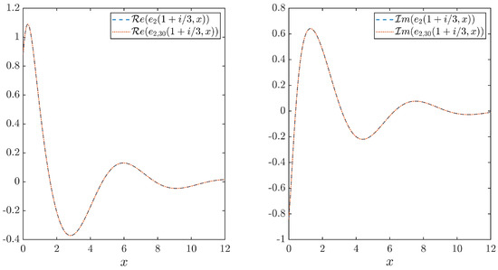
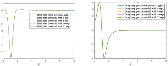
Figure 1 shows the real and imaginary parts of the approximate and exact Jost solution computed from (36) at a sample point $\rho =1+i/3$ with $N=30$, i.e., $e_{2,30}(1+i/3,x)$. The maximum absolute error of the computed Jost solution for x in the interval $[0,12]$ is $2.14\times {10}^{-13}.$

Figure 1. Real (left) and imaginary (right) parts of $e_2(1+i/3,x)$ and approximate Jost solution $e_{2,30}(1+i/3,x)$.

Table 2 presents the maximum absolute and relative errors of the approximate Jost function $e_{2,N}\left(\rho \left(z\right)\right)$ for $z\in \overline{\mathbb{D}}$ for different values of N.

Table 2. Maximum absolute and relative errors of the approximate Jost function $e_{2,N}\left(\rho \left(z\right)\right)$ in $\overline{\mathbb{D}}$.

N	2	5	20	25	30	40	180
Abs. Error	$1.57\times {10}^{-1}$	$5.82\times {10}^{-3}$	$4.06\times {10}^{-10}$	$1.68\times {10}^{-12}$	$2.48\times {10}^{-14}$	$1.98\times {10}^{-14}$	$1.96\times {10}^{-14}$
Rel. Error	$1.78\times 10$	$6.58\times {10}^{-1}$	$4.58\times {10}^{-8}$	$1.89\times {10}^{-10}$	$9.66\times {10}^{-13}$	$3.17\times {10}^{-13}$	$1.57\times {10}^{-13}$

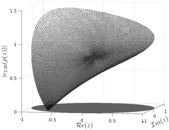
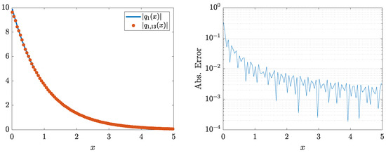
Figure 2 shows the function $\left|e_{2,30}\left(\rho \left(z\right)\right)\right|$ for $z\in \overline{\mathbb{D}}$. Here, we illustrate the existence of a unique singular number. Indeed, this singular number $\rho =-1$ corresponds to $z=-0.6-0.8i$ and the value $e_{2,30}(-1)$ is $-5.55\times {10}^{-15}+2.66\times {10}^{-15}i$.

Figure 2. Function $\left|e_{2,30}\left(\rho \left(z\right)\right)\right|$ for $z\in \overline{\mathbb{D}}$.

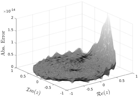
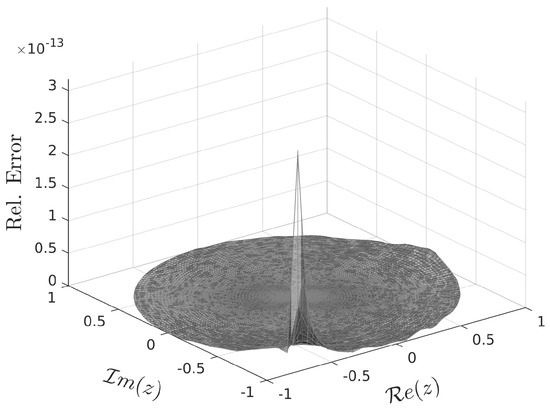
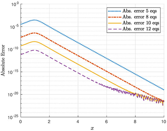
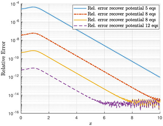
The distribution of the absolute and relative errors of the approximate Jost function is presented in Figure 3 and Figure 4 (respectively), where the maximum absolute error is $1.98\times {10}^{-14}$ and the maximum relative error is $3.17\times {10}^{-13}$.

Figure 3. Absolute error of approximate Jost function $e_{2,30}\left(\rho \left(z\right)\right)$ for $z\in \overline{\mathbb{D}}$.

Figure 4. Relative error of approximate Jost function $e_{2,30}\left(\rho \left(z\right)\right)$ for $z\in \overline{\mathbb{D}}$.

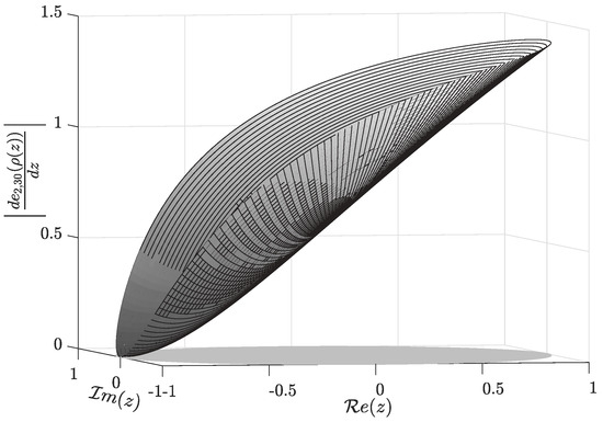
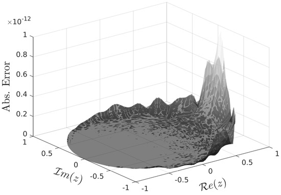
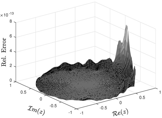
Furthermore, a good approximation of the derivative of the Jost function becomes essential for the argument principle algorithm performance. This is necessary to obtain the eigenvalues as the squares of non-real zeros of the approximate Jost function. In Figure 5, we illustrate $\frac{d{e}_{2,30}\left(\rho \left(z\right)\right)}{dz}$, and Figure 6 and Figure 7 depict the distribution of the absolute and relative errors, respectively. The maximum absolute error is $9.6\times {10}^{-13}$ and the maximum relative error is $7.21\times {10}^{-13}$.

Figure 5. Function $\left|\frac{d{e}_{2,30}\left(\rho \left(z\right)\right)}{dz}\right|$ for $z\in \overline{\mathbb{D}}$.

Figure 6. Absolute error of $\frac{d{e}_{2,30}\left(\rho \left(z\right)\right)}{dz}$, $z\in \overline{\mathbb{D}}$.

Figure 7. Relative error of $\frac{d{e}_{2,30}\left(\rho \left(z\right)\right)}{dz}$, $z\in \overline{\mathbb{D}}$.

To find the singular numbers, we consider the circle $\left\{z\in \mathbb{C}:\left|z\right|=1\right\}$ (real axis in ρ) and a cubic spline interpolation of the approximate Jost function ($N=30$). For the spline interpolation, we use the Matlab routine csapi. To locate the zeros of the spline, we use slmsolve from the Shape Language Modeling (SLM) toolbox, version 1.14 by John D’Errico [59], available for Matlab2021a. The value ${\rho }_1=-1.000000000000003$ was obtained with an absolute error of $3.11\times {10}^{-15}.$ Additionally, the argument principle algorithm applied to $e_{2,30}\left(\rho \left(z\right)\right)$ in $\mathbb{D}$ discarded any eigenvalue of the problem (non-real zero ρ).

The second step of the algorithm from Section 3.4 requires computing the Jost function in the strip $-{\epsilon }_0<Im\left(\rho \right)<0$ (${\epsilon }_0=\frac{\epsilon }{2}=1$). In this example, we extend $e_{2,30}\left(\rho \left(z\right)\right)$ analytically via Padé’s approximation. The Padé approximant ${\left[m,n\right]}_{e_{2,30}\left(\rho \right)}$ was computed in Matlab2021a using the routine pade.

In Table 3, we computed the maximum absolute and relative errors of the Padé approximant ${\left[1,1\right]}_{e_{2,N}\left(\rho \right)}$ of $e_{2,N}\left(\rho \right)$ with $N=3,5,20,30,40,50\mathrm{and}180$ for $0\le Im\left(\rho \right)<1$. These values indicate the possibility of dealing with this Padé approximant when computing the set of scattering data. Additionally, from Table 4, we confirm that this approximant satisfactorily extends the Jost function to a desirable strip in the lower half-plane (the strip is related to the one needed for the calculation of the scattering function $s_2\left(\rho \right)$).

Table 3. Maximum absolute and relative errors of the Padé approximant ${\left[1,1\right]}_{e_{2,N}\left(\rho \right)}$ with respect to $e_{2,N}\left(\rho \right)$ in a strip in the upper half $\rho$-plane.

N	Max. Abs. Error of ${\left[1,1\right]}_{{\mathit{e}}_{2,\mathit{N}}\left(\mathit{\rho }\right)}\left(\mathit{\rho }\right)$	N	Max. Rel. Error of ${\left[1,1\right]}_{{\mathit{e}}_{2,\mathit{N}}\left(\mathit{\rho }\right)}\left(\mathit{\rho }\right)$
	with $0\le Im\left(\mathit{\rho }\right)<1$		with $0\le Im\left(\mathit{\rho }\right)<1$
3	$7.18\times {10}^{-1}$	3	$2.97$
5	$5.45\times {10}^{-1}$	5	$2.14$
20	$1.26\times {10}^{-6}$	20	$4.3\times {10}^{-6}$
30	$4.6\times {10}^{-11}$	30	$1.58\times {10}^{-10}$
40	$8.71\times {10}^{-12}$	40	$3.10\times {10}^{-11}$
50	$1.93\times {10}^{-11}$	50	$6.56\times {10}^{-11}$
180	$1.05\times {10}^{-10}$	180	$3.56\times {10}^{-10}$

Table 4. Maximum absolute and relative errors of the Padé approximant ${\left[1,1\right]}_{e_{2,N}\left(\rho \right)}$ with respect to the exact Jost function $e_2\left(\rho \right)$ in a strip in the lower half $\rho$-plane.

N	Max. Abs. Error of ${\left[1,1\right]}_{{\mathit{e}}_{2,\mathit{N}}\left(\mathit{\rho }\right)}\left(\mathit{\rho }\right)$	N	Max. Rel. Error of ${\left[1,1\right]}_{{\mathit{e}}_{2,\mathit{N}}\left(\mathit{\rho }\right)}\left(\mathit{\rho }\right)$
	in $-1<Im\left(\mathit{\rho }\right)\le 0$		in $-1<Im\left(\mathit{\rho }\right)\le 0$
3	$3.07$	3	$2.99$
5	$2.66$	5	$2.16$
20	$7.99\times {10}^{-6}$	20	$4.34\times {10}^{-6}$
30	$2.89\times {10}^{-10}$	30	$1.59\times {10}^{-10}$
40	$5.65\times {10}^{-11}$	40	$3.12\times {10}^{-11}$
50	$1.23\times {10}^{-10}$	50	$6.61\times {10}^{-11}$
180	$6.54\times {10}^{-10}$	180	$3.59\times {10}^{-10}$

To obtain $s_2\left(\rho \right)$ numerically on the strip $0<Im\left(\rho \right)<{\epsilon }_0=1$, we use the truncated series $e_{2,30}\left(\rho \right)$ and the Padé approximant ${\left[1,1\right]}_{e_{2,30}\left(\rho \right)}$:

$$s_2\left(\rho \right)\approx \frac{{\left[1,1\right]}_{e_{2,30}\left(\rho \right)}(-\rho )}{e_{2,30}\left(\rho \right)}.$$

The maximum absolute error inside the region $\mathcal{R}=[-30,30]\times \left[{10}^{-2}i,\left({\epsilon }_0-{10}^{-2}\right)i\right]$ is $9.64\times {10}^{-10}$.

Remark 14. 

The order of the Padé approximant used for the Jost function is not arbitrary. Although the maximum absolute errors inside the region $\mathcal{R}$ of other approximations of $s_2\left(\rho \right)$ using ${[2,2]}_{e_{2,30}\left(\rho \right)}\left(9.35\times {10}^{-11}\right)$, ${[3,3]}_{e_{2,30}\left(\rho \right)}$ $\left(1.34\times {10}^{-11}\right)$, ${[4,4]}_{e_{2,30}\left(\rho \right)}$ $\left(1.5\times {10}^{-11}\right)$ and ${[7,7]}_{e_{2,30}\left(\rho \right)}$ $\left(6.37\times {10}^{-12}\right)$ are better in comparison with ${[1,1]}_{e_{2,30}\left(\rho \right)}$, we choose ${[1,1]}_{e_{2,30}\left(\rho \right)}$ as the most suitable option to avoid the appearance of Froissart doublets. Indeed, the use of the Padé approximants when there is no available information about the smoothness of the function to be approximated is challenging. Some publications propose modified algorithms [60], even using the Toeplitz matrix theory with many numerical implementations in Maple, Wolfram Mathematica (see [61]) or Matlab (see [62]). For the purposes of this paper, it is sufficient to use only the information obtained from the truncated series $e_N\left(\rho \right)$ and the argument principle algorithm to construct the approximant. Consider the number K of zeros counting multiplicities of the approximate Jost function $e_N\left(\rho \right)$ (singular numbers being calculated using the argument principle algorithm) located inside $\mathbb{D}$ as the degree of the polynomial in the numerator in the Padé approximant. Recalling that, in most cases, an accurate Padé’s approximation is obtained on the diagonal approximant types for analytical functions, it is reasonable to choose the Padé approximant as ${[K,K]}_{e_N\left(\rho \right)}$.

Example 10. 

Consider the potential $q_3\left(x\right)$ from Example 3. The approximate Jost function $e_{3,N}\left(\rho \right)$ is computed in the strip $0\le Im\left(\rho \right)<\frac{\epsilon }{2}=1$ for several values of N. In Table 5, the maximum absolute error of the approximate Jost function is presented.

Table 5. Maximum absolute error of the Jost function $e_{3,N}\left(\rho \right)$ for $N=2,5,20,30,50$ and 180.

N	2	5	20	30	50	180
Abs. Error	$2.34\times {10}^{-1}$	$8.65\times {10}^{-3}$	$6.03\times {10}^{-10}$	$5.57\times {10}^{-14}$	$4.72\times {10}^{-14}$	$4.67\times {10}^{-14}$

Similarly to the previous example, a search for real singular numbers was performed; however, none were detected. Subsequently, the argument principle algorithm located a non-real singular number in $\mathbb{D}$, with the value $z_1\approx -0.386709149322063-0.105221869864471i$ (${\rho }_1\approx -0.271752585319512+1.083923327338694i$). Its absolute error is $8\times {10}^{-15}$. The contour refinement is not a concern, since the performed algorithm from [54] is based on the argument principle algorithm followed by several Newton iterations.

Additionally, the Jost function was extended to the strip $\left|Im\left(\rho \right)\right|<{\epsilon }_0=1$ through the Padé approximant

$${\left[1,1\right]}_{e_{3,30}\left(\rho \right)}=\frac{\rho \left(4.69\times {10}^{15}+4.94\times {10}^{13}i\right)+1.94\times {10}^{15}-4.92\times {10}^{15}i}{\rho \left(4.69\times {10}^{15}+6.12\times {10}^{14}i\right)-6.11\times {10}^{14}+4.69\times {10}^{15}i}.$$

The corresponding maximum absolute error of ${\left[1,1\right]}_{e_{3,30}\left(\rho \right)}\left(\rho \right)$ inside the rectangle ${\mathcal{R}}_1:=[-20,20]\times \left[0i,\left({\epsilon }_0-{10}^{-2}\right)i\right]$ in the complex ρ-plane is $8.43\times {10}^{-11}$. Inside ${\mathcal{R}}_2:=[-20,20]\times \left[\left(-{\epsilon }_0+{10}^{-2}\right)i,\left({\epsilon }_0-{10}^{-2}\right)i\right]$, the maximum absolute error is $8.42\times {10}^{-11}$.

Next, an approximate value of the normalization constant corresponding to ${\rho }_1$ was computed

$$c_1\approx \frac{{\left[1,1\right]}_{e_{3,30}\left(\rho \right)}(-{\rho }_1)}{\dot{e}{}_{3,30}\left({\rho }_1\right)}i\approx -10.317711295453737+12.894194226972697i$$

with an absolute error of $2.8\times {10}^{-9}.$

Finally, we calculate the scattering function by

$$s_3\left(\rho \right)\approx \frac{{\left[1,1\right]}_{e_{3,30}\left(\rho \right)}(-\rho )}{e_{3,30}\left(\rho \right)}.$$

(107)

The maximum absolute error of the approximation of $s_3\left(\rho \right)$ in ${\mathcal{R}}_1$ is $1\times {10}^{-9}$ (see Figure 8).

Figure 8. Absolute error of the approximate scattering function $s_3\left(\rho \right)\approx \frac{{\left[1,1\right]}_{e_{3,30}\left(\rho \right)}(-\rho )}{e_{3,30}\left(\rho \right)}$.

Example 11. 

Consider the potential $q_1\left(x\right)$ from Example 1. Table 6 shows the parameter ${\epsilon }_N$ for some values of $N.$

Table 6. Example 11: parameter ${\epsilon }_N$ for different values of N.

N	${\mathit{\epsilon }}_{\mathit{N}}$ for $\mathit{x}\in [0,12]$	N	${\mathit{\epsilon }}_{\mathit{N}}$ for $\mathit{x}\in [0,12]$
2	$4.43$	38	$1.12\times {10}^{-5}$
3	$2.91$	48	$6.97\times {10}^{-7}$
5	$1.13$	58	$5.17\times {10}^{-8}$
10	$1.32\times {10}^{-1}$	88	$4.46\times {10}^{-11}$
15	$1.88\times {10}^{-2}$	98	$5.12\times {10}^{-12}$
20	$3.17\times {10}^{-3}$	108	$9.48\times {10}^{-13}$
28	$2.27\times {10}^{-4}$	178	$1.49\times {10}^{-12}$

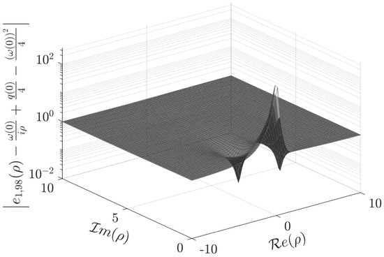
Note that the approximation of the Jost function in this example requires more terms in the series representation than in previous examples. To control the accuracy of the approximation, in addition to the parameter ${\epsilon }_N$, one can use the asymptotic relation for the Jost function from [24] (p. 105),

$$e\left(\rho \right)=1+\frac{\omega \left(0\right)}{i\rho }-\frac{q\left(0\right)}{{\left(2i\rho \right)}^2}+\frac{{\omega }^2\left(0\right)}{{\left(2i\rho \right)}^2}+o\left(\frac{1}{{\rho }^2}\right),\left|\rho \right|\to \infty ,\rho \in {\mathbb{C}}^{+}\setminus \left\{0\right\},$$

(108)

where $\omega \left(x\right)=-\frac{1}{2}{\int }_x^{\infty }q\left(s\right)ds$. This relation is valid for $q\left(x\right)$ with first and second summable derivatives.

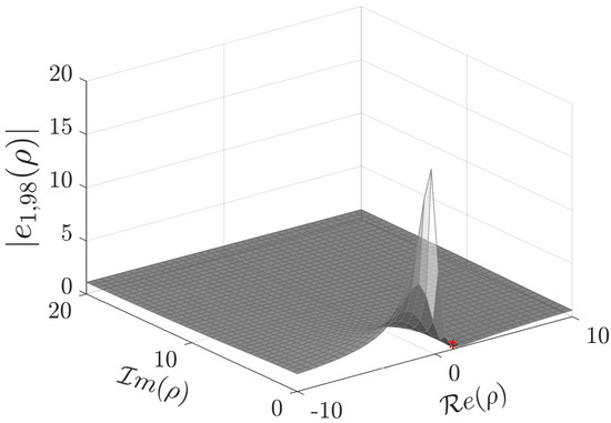
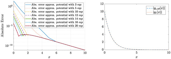
Figure 9 depicts the Jost function computed with $N=98$ and the singular number ${\rho }_0\approx 1.784065846059995+0.608788673578742i$. Figure 10 shows the fulfillment of the asymptotic relation (108), namely the graph of $\left|e_{1,98}\left(\rho \right)-\frac{\omega \left(0\right)}{i\rho }+\frac{q\left(0\right)}{{\left(2i\rho \right)}^2}-\frac{{\omega }^2\left(0\right)}{{\left(2i\rho \right)}^2}\right|$, which tends to 1 when $\left|\rho \right|\to \infty$.

Figure 9. Absolute value of $e_{1,98}\left(\rho \right)$ in the upper half $\rho$-plane. The marked point is the singular number ${\rho }_0$.

Figure 10. Graph of $\left|e_{1,98}\left(\rho \right)-\frac{\omega \left(0\right)}{i\rho }+\frac{q\left(0\right)}{{\left(2i\rho \right)}^2}-\frac{{\omega }^2\left(0\right)}{{\left(2i\rho \right)}^2}\right|$ tending to 1 when $\left|\rho \right|\to \infty$.

The eigenvalue is computed numerically as a zero of the exact Jost function with the aid of Wolfram Mathematica v.12 (Wolfram Research, Inc., Champaign, IL, USA) ${\lambda }_0\approx {\lambda }_0^{*}:=2.8122672899483+2.1722381890043i$. This “exact” eigenvalue is compared with the approximation $2.812267289948449+2.172238189004328i$ obtained as the square of the approximate ${\rho }_0$. The absolute error is $1.52\times {10}^{-13}$.

For the numerical calculation of the analytic extension of $e_{1,98}\left(\rho \right)$ onto the strip $-\frac{1}{2}<Im\left(\rho \right)<0$, it is not possible to consider the Padé approximant ${[1,1]}_{e_{1,98}\left(\rho \right)}$. This does not approximate $e_{1,98}\left(\rho \right)$ accurately even in the upper half-plane of the complex variable ρ. Using the Padé approximant ${[7,7]}_{e_{1,98}\left(\rho \right)}$ the absolute error was $0.17$.

Instead of using Formula (105) to compute the normalization constant $c_0$, Formula (104) is applied to obtain the approximation $c_0\approx 16.339391965970112+40.670169715260290i$ with absolute error $3.05\times {10}^{-12}.$

To compute the scattering function $s_1\left(\rho \right)$ on a line parallel to the real axis contained in the strip $\left|Im\left(\rho \right)\right|<{\epsilon }_0=\left|Im\left({\rho }_0\right)\right|\approx 0.608788673578742i$, Formula (106) was used. The function $e_1\left(\rho \right)$ is represented by (36) for ρ on a line in the lower half ρ-plane parallel and sufficiently close to the real axis. Having calculated these series representations for the functions involved in $s_1\left(\rho \right),$ we compute

$$s_1\left(\rho \right)\approx \frac{e_{1,98}(-\rho )}{e_{1,98}\left(\rho \right)}$$

with a maximum absolute error $1.45\times {10}^{-7}$ along the line ${\mathcal{L}}_{\eta =0.1}$ (see (77)).

In this example, we obtain a satisfactory accuracy in the calculations of the scatterin data set using the expression (36) alone and the derivatives required by (104).

Example 12

([44]). Consider the potential

$$q_4\left(x\right):=Risin\left(x\right)e^{-x},$$

with R being a constant (Reynolds number). When $R>0$ is sufficiently large, the eigenvalues may exist. For example, for $R=10$, there is one eigenvalue in the box $\mathcal{B}:=1.{6043912}_{44}^{58}+1.7978849i_{67}^{81}$ [44] (see also [45]).

The Jost solution is not available in a closed form. In order to check the validity of the numerical calculation of the coefficients $a_n\left(x\right)$ for $e_{4,N}(\rho .x)$, we consider the indicator ${\epsilon }_N$ (Table 7).

Table 7. Example 12: indicator ${\epsilon }_N$ for different values of N (potential $q_4\left(x\right)$ with $R=10$).

N	${\mathit{\epsilon }}_{\mathit{N}}$ for $\mathit{x}\in [0,12]$	N	${\mathit{\epsilon }}_{\mathit{N}}$ for $\mathit{x}\in [0,12]$
2	$4.43$	55	$3.92\times {10}^{-7}$
3	$2.91$	105	$9.77\times {10}^{-11}$
5	$5.97\times {10}^{-1}$	136	$1.06\times {10}^{-12}$
10	$7.85\times {10}^{-2}$	137	$9.19\times {10}^{-13}$
15	$1.17\times {10}^{-2}$	155	$6.11\times {10}^{-13}$
20	$1.70\times {10}^{-3}$	175	$7.77\times {10}^{-13}$
45	$6.95\times {10}^{-6}$	200	$9.72\times {10}^{-13}$

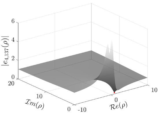
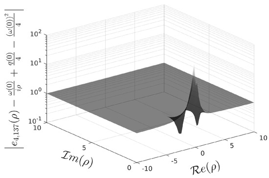
Figure 11 depicts the Jost function computed with $N=137$ and the approximation of the singular number ${\rho }_1\approx 1.416695330664399+0.634534798062634i$, with its square belonging to the box $\mathcal{B}$. Additionally, Figure 12 shows the fulfillment of the asymptotic relation (108).

Figure 11. Absolute value of $e_{4,137}\left(\rho \right)$ ($R=10$) in the upper half $\rho$-plane and the marked point is the approximate singular number ${\rho }_1$.

Figure 12. Graph of $\left|e_{4,137}\left(\rho \right)-\frac{\omega \left(0\right)}{i\rho }+\frac{q\left(0\right)}{{\left(2i\rho \right)}^2}-\frac{{\omega }^2\left(0\right)}{{\left(2i\rho \right)}^2}\right|$ tending to 1 when $\left|\rho \right|\to \infty$ ($R=10$).

The normalization constant $c_1$ is calculated using (104),

$$c_1\approx 0.423317609673475+10.608764849282464i.$$

Finally, the scattering function is approximated by ${\displaystyle \frac{e_{4,137}(-\rho )}{e_{4,137}\left(\rho \right)}}$.

Now, take $R=30$ in the potential $q_4\left(x\right)$. In this case, two boxes localizing the only two eigenvalues ${\lambda }_1$ and ${\lambda }_2$ were obtained in [44],

$${\mathcal{B}}_1:={2.555641614}_{19}^{35}+{7.688187018}_{03}^{19}i,{\mathcal{B}}_2:={6.37465}_{12}^{91}+{2.4699}_{46}^{55}i.$$

Table 8 provides the values of the indicator ${\epsilon }_N$ for several values of N.

Table 8. Example 12: indicator ${\epsilon }_N$ for different values of N ($R=30$).

N	${\mathit{\epsilon }}_{\mathit{N}}$ for $\mathit{x}\in [0,12]$	N	${\mathit{\epsilon }}_{\mathit{N}}$ for $\mathit{x}\in [0,12]$
5	$1.09\times {10}^1$	105	$1.27\times {10}^{-7}$
10	$2.86$	155	$2.30\times {10}^{-10}$
15	$7.71\times {10}^{-1}$	175	$2.78\times {10}^{-11}$
20	$1.17\times {10}^{-1}$	200	$5.70\times {10}^{-12}$
45	$1.66\times {10}^{-3}$	220	$6.46\times {10}^{-12}$
55	$1.65\times {10}^{-4}$	230	$7.04\times {10}^{-12}$

Approximate eigenvalues computed from $e_{4,N}\left(\rho \right)$ for different values of N, are presented in Table 9 and Table 10.

Table 9. Approximate eigenvalue ${\tilde{\lambda }}_1$ computed using different values of N in $e_{4,N}\left(\rho \right)$ ($R=30$).

N	${\tilde{\mathit{\lambda }}}_1$
35	2.555647790300414 + 7.688132784089897i
65	2.555641614022092 + 7.688187017680658i
105	2.555641614273991 + 7.688187018110548i
200	2.555641614273991 + 7.688187018110548i
230	2.555641614273991 + 7.688187018110548i

Table 10. Approximate eigenvalue ${\tilde{\lambda }}_2$ computed using different values of N in $e_{4,N}\left(\rho \right)$ ($R=30$).

N	${\tilde{\mathit{\lambda }}}_2$
35	6.368733224187178 + 2.460948309337657i
65	6.374657558248066 + 2.460950123973226i
105	6.374654410969357 + 2.460950093296220i
200	6.374654410861196 + 2.460950093077938i
230	6.374654410861196 + 2.460950093077938i

Note that ${\tilde{\lambda }}_1\in {\mathcal{B}}_1$ and ${\tilde{\lambda }}_2\in {\mathcal{B}}_2$ for $N=200$. Finally, the normalization constants are calculated using $e_{4,200}\left(\rho \right)$ in (104),

$$\begin{array}{cc}\hfill c_1& \approx 1.669128547357084\times {10}^2-1.694940279771396\times {10}^{2}i\hfill \\ \hfill c_2& \approx -54.578951306154920+45.276710620944780i.\hfill \end{array}$$

Although, in this example, more powers for the series representation of the Jost function were used, the method proved to be applicable to obtaining the scattering data set without any additional informatio. The good accuracy achieved is confirmed by the ability t use the scattering data obtained as input data to solve the inverse scattering problem to recover the potential $q_4\left(x\right)$ with $R=30$ below in Example 22.

5.2. Inverse Problem

In the present section, we discuss the accuracy, convergence and stability of the proposed method for solving the inverse scattering problem.

Remark 15. 

By $q_{k,M}\left(x\right)$, we denote the approximation of the potential $q_k\left(x\right)$ ($k=1,2,3,4,5$) obtained by solving the truncated system (100) with the sum up to M, i.e., with $M+1$ equations.

5.2.1. Convergence and Accuracy

Example 13. 

Consider the scattering data calculated in Example 3:

$$J=\left\{\left\{{\rho }_1=itanh(1+i),m_1=1,c_1=\frac{2(i+itanh(1+i\left)\right)tanh(1+i)}{i-itanh(1+i)}\right\},\right.$$

$$\left.s_3\left(\rho \right)=\frac{\left(\rho +itanh(1+i)\right)\left(\rho +i\right)}{\left(\rho -itanh(1+i)\right)\left(\rho -i\right)}\right\}$$

where $s_3\left(\rho \right)$ is an S-type function in the strip $0\le \left|Im\left(\rho \right)\right|<{\epsilon }_0=1$.

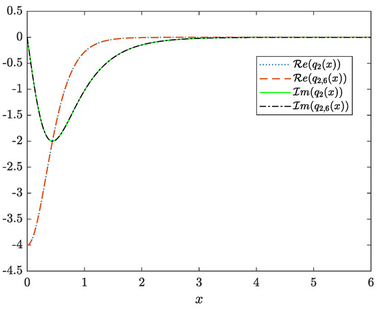
We shall recover the potential $q_3\left(x\right)=-2{sech}^2(x-1-i).$ The system (100) of linear algebraic equations for this example is obtained in a closed form (see Example 7). For a different number of equations in the truncated system, we obtain a solution symbolically by using the Matlab routine solve. The potential $q_3\left(x\right)$ is recovered from (38). Figure 13 presents the recovered potential in each case.

Figure 13. Real (left) and imaginary (right) part of the recovered potential $q_{3,M}\left(x\right)$ for $M=4,7,9$ and 11.

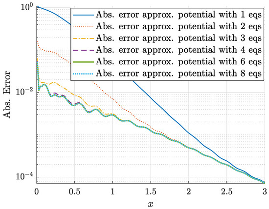
The corresponding absolute and relative errors are presented in Figure 14 and Figure 15, respectively. Note that a high accuracy is attained even in the case of a very reduced number of equations in the truncated system. Moreover, a very fast convergence of the method can be appreciated.

Figure 14. Absolute error of the recovered potential $q_{3,M}\left(x\right)$ with $M=4,7,9$ and 11.

Figure 15. Relative error of the recovered potential $q_{3,M}\left(x\right)$ with $M=4,7,9$ and 11.

Example 14. 

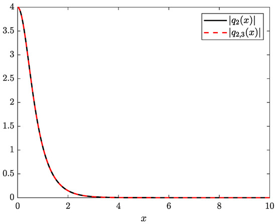
Consider the scattering data $J=\left\{s_2\left(\rho \right)\right\}$ from Example 2. As was shown above (Example 6), the system (100) for this example can be written explicitly. Again, when solving the corresponding truncated system for different values of M we observe a fast convergence and remarkable accuracy even for small values of M (see Table 11 and Figure 16).

Table 11. Maximum absolute error of the approximate potential $q_{2,M}\left(x\right)$ for some values of M.

M in (100)	0	1	2	3	6	8
${\displaystyle \underset{x\in [0,6]}{max}\left|q_2\left(x\right)-q_{2,M}\left(x\right)\right|}$	$1.05$	$1.13\times {10}^{-1}$	$1.25\times {10}^{-2}$	$1.4\times {10}^{-3}$	$1.91\times {10}^{-6}$	$2.35\times {10}^{-8}$

Figure 16. Exact and computed potential $q_{2,6}\left(x\right)$.

Example 15. 

Consider the closed form of the scattering function $s_1\left(\rho \right)$ from Example 1. We compute functions $f_{m,c}\left(x\right)$ and $A_{mn,c}\left(x\right)$ using the first option from Remark 11. Some poles and residues are given in Table 12 (computed with the aid of the package Numerical Calculus of Mathematica v.12).

Table 12. Poles and residues in the upper half-plane of the function $s_1\left(\rho \right)-1$.

Poles	Residues
$0.5i$	5
$1.784065846059995+0.608788673578742i$	$40.670169841396-16.339391035537i$
$1i$	$-25i$
$1.5i$	$-\frac{125}{3}$
$2i$	$\frac{625}{18}i$
$2.5i$	$\frac{625}{36}$
$3i$	$-\frac{625}{108}i$
$3.5i$	$-\frac{1743}{1265}$
$4i$	$\frac{249}{1012}i$
$6i$	$\frac{7}{267,683}i$
$7i$	$-\frac{1}{10,857,221}i$

Note that the absolute value of the residues decreases considerably as the poles move away from the origin on the imaginary axis. This allows us to use a small number of poles for the calculation of the functions $f_{m,c}\left(x\right)$ and $A_{mn,c}\left(x\right)$.

The convergence of the method in this case results to be slower; see Figure 17, although a satisfactory accuracy is attained for $M=9$.

Figure 17. Absolute error for different values of M in the truncated system (100) (left) and the absolute value of the recovered potential $q_{1,19}\left(x\right)$ computed with 20 equations (right) for $x\in [0,10]$.

5.2.2. Stability of the System

Since the stability of the method was proved in Theorem 4, we are able to work efficiently with noisy scattering data. First, we consider the natural noise arising from the numerical implementations of the last two procedures in Remark 11, i.e., calculation of the approximate matrix in (100) from the scattering function $s\left(\rho \right)$ given in a closed form. Another situation considered in this subsection is the recovery of the potential from a uniformly noisy scattering function.

Remark 16. 

Henceforth, denote by ${\tilde{f}}_m\left(x\right)$, ${\tilde{f}}_{m,c}\left(x\right)$, ${\tilde{A}}_{mn}\left(x\right)$ and ${\tilde{A}}_{mn,c}\left(x\right)$ the numerical approximation of $f_m\left(x\right)$, $f_{m,c}\left(x\right)$, $A_{mn}\left(x\right)$ and $A_{mn,c}\left(x\right)$.

Remark 17. 

In the last step of the algorithm from Section 4.4, for recovering q with the aid of (38), the coefficient $a_0$ needs to be differentiated twice. This was performed by interpolating $a_0\left(x\right)$ with a quintic spline through the Matlab routine spapi and a posterior differentiation with the Matlab command fnder.

Example 16. 

Let us consider the scattering data from Example 2. The recovery of the potential $q_2\left(x\right)$ from the exact scattering function $s_2\left(\rho \right)$, obtained by using approximate functions ${\tilde{f}}_m\left(x\right)$ and ${\tilde{A}}_{mn}\left(x\right)$ in the truncated system (100), is presented. The computation of functions $f_m\left(x\right)$ and $A_{mn}\left(x\right)$ requires numerical integration along the line ${\mathcal{L}}_{\eta =0.5}$ (see (77)). For this purpose, the last two procedures in Remark 11 were applied.

Method 1. The second option in Remark 11 is implemented. With the scattering function (91) at points $\rho =\sigma +0.5i$ and $\sigma =-(k+1/2)h$ for $k=0,1,\dots ,N\left(x\right)$, where $N\left(x\right)=55000/x$ and $h=0.145454545$, the calculation of the Fourier transforms in (98) is carried out. In Table 13, the maximum absolute error of ${\tilde{f}}_m\left(x\right)$ is presented for 4 values of the parameter m.

Table 13. Example 16: maximum absolute error of ${\tilde{f}}_{m,c}\left(x\right)$ calculated with the second procedure in Remark 11.

m	0	1	2	3
${\displaystyle \underset{x\in (0,20)}{max}\left|f_m\left(x\right)-{\tilde{f}}_m\left(x\right)\right|}$	$1.102\times {10}^{-9}$	$7.995\times {10}^{-10}$	$7.988\times {10}^{-10}$	$8.757\times {10}^{-10}$

Now, we compute ${\tilde{A}}_{mn,c}\left(x\right)$ using the same numerical integration method with parameters $N\left(x\right)=5500/x$ and $h=0.127272727$.

Table 14 shows the maximum absolute error of ${\tilde{A}}_{mn}\left(x\right)$ for parameters $m,n=0,1,2,3$.

Table 14. Example 16: maximum absolute error of ${\tilde{A}}_{mn}\left(x\right)$ calculated with the second procedure in Remark 11.

m	${\displaystyle \underset{\mathit{x}\in (0,20)}{max}\left|{\mathit{A}}_{\mathit{mn}}\left(\mathit{x}\right)-{\tilde{\mathit{A}}}_{\mathit{mn}}\left(\mathit{x}\right)\right|}$
	$\mathit{n}=\mathbf{0}$	$\mathit{n}=\mathbf{1}$	$\mathit{n}=\mathbf{2}$	$\mathit{n}=\mathbf{3}$
0	$4.721\times {10}^{-10}$	$4.712\times {10}^{-10}$	$4.711\times {10}^{-10}$	$4.714\times {10}^{-10}$
1	$4.712\times {10}^{-10}$	$4.711\times {10}^{-10}$	$4.714\times {10}^{-10}$	$4.712\times {10}^{-10}$
2	$4.711\times {10}^{-10}$	$4.714\times {10}^{-10}$	$4.712\times {10}^{-10}$	$4.699\times {10}^{-10}$
3	$4.714\times {10}^{-10}$	$4.712\times {10}^{-10}$	$4.699\times {10}^{-10}$	$4.678\times {10}^{-10}$

The system (100) constructed with ${\tilde{f}}_m\left(x\right)$ and ${\tilde{A}}_{mn}\left(x\right)$ is solved numerically in Matlab for several values of M. Maximum absolute and relative errors of the approximation of the potential $q_{2,M}$ are shown in Table 15.

Table 15. Example 16: maximum absolute and relative errors of the approximation of the potential $q_{2,M}\left(x\right)$ by the recovered potential for some values of M in (100).

M in (100)	0	1	2	3	5	7
Abs. Error of $q_{2,M}\left(x\right)$	$9.3\times 10{}^{-1}$	$1\times {10}^{-1}$	$1.1\times {10}^{-2}$	$1.21\times {10}^{-3}$	$1.06\times {10}^{-4}$	$1.14\times {10}^{-4}$
Rel. Error of $q_{2,M}\left(x\right)$	$1.6$	$1.74\times {10}^{-2}$	$1.93\times {10}^{-3}$	$2.14\times {10}^{-4}$	$4.15\times {10}^{-6}$	$2.04\times {10}^{-6}$

Figure 18 presents the absolute value of the recovered $q_2$ potential from 4 equations in (100).

Figure 18. Recovered potential $q_{2,3}\left(x\right)$ by Method 1 in Example 16.

Method 2. Now, we compute the approximate functions ${\tilde{f}}_m\left(x\right)$ (see Table 16) and ${\tilde{A}}_{mn}\left(x\right)$ (see Table 17) following the third procedure in Remark 11.

Table 16. Example 16: maximum absolute error of ${\tilde{f}}_m\left(x\right)$ after applying the third procedure in Remark 11.

m	0	1	2	3
${\displaystyle \underset{x\in (0,20)}{max}\left|f_m\left(x\right)-{\tilde{f}}_m\left(x\right)\right|}$	$6.05\times {10}^{-5}$	$2.02\times {10}^{-5}$	$6.73\times {10}^{-6}$	$2.24\times {10}^{-6}$

Table 17. Example 16: maximum absolute error of ${\tilde{A}}_{mn}\left(x\right)$ after applying the third procedure in Remark 11.

m	${\displaystyle \underset{\mathit{x}\in (0,20)}{max}\left|{\mathit{A}}_{\mathit{mn}}\left(\mathit{x}\right)-{\tilde{\mathit{A}}}_{\mathit{mn}}\left(\mathit{x}\right)\right|}$
	$\mathit{n}=\mathbf{0}$	$\mathit{n}=\mathbf{1}$	$\mathit{n}=\mathbf{2}$	$\mathit{n}=\mathbf{3}$
0	$1.27\times {10}^{-13}$	$4.26\times {10}^{-14}$	$1.42\times {10}^{-14}$	$4.74\times {10}^{-15}$
1	$1.22\times {10}^{-9}$	$1.42\times {10}^{-14}$	$4.74\times {10}^{-15}$	$1.58\times {10}^{-15}$
2	$4.07\times {10}^{-10}$	$1.36\times {10}^{-10}$	$1.58\times {10}^{-15}$	$5.29\times {10}^{-16}$
3	$1.36\times {10}^{-10}$	$4.52\times {10}^{-11}$	$1.5\times {10}^{-11}$	$1.68\times {10}^{-12}$

In Table 18, the absolute error of the recovered potential for some values of M in (100) is presented.

Table 18. Example 16: maximum absolute error of recovered potential $q_{2,M}\left(x\right)$ using the third option in Remark 11.

M in (100)	0	1	2	3	5	7
${\displaystyle \underset{x\in (0,20)}{max}\left|q_2\left(x\right)-q_{2,M}\left(x\right)\right|}$	$8.25\times {10}^{-1}$	$2.34\times {10}^{-1}$	$5.25\times {10}^{-2}$	$9.71\times {10}^{-3}$	$5.71\times {10}^{-3}$	$2.23\times {10}^{-3}$
Rel. Error of $q_{2,M}\left(x\right)$	$1.24$	$1.21\times {10}^{-1}$	$5.2\times {10}^{-1}$	$8\times {10}^{-2}$	$6.19\times {10}^{-2}$	$7.25\times {10}^{-3}$

Both methods (procedures 2 and 3 from Remark 11) illustrated in the above example have proven to be suitable for calculating the functions $f_m$ and $A_{mn}$ from a table of values for the $s_2\left(\rho \right)$. Nevertheless, it is worth mentioning that although the first method (procedure 2) produced slightly more accurate results, this approach might be sensitive to the choice of the $N\left(x\right)$ and h parameters, whereas the second method (procedure 3) only requires the implementation of trapz, the Matlab integration routine on a dense set of points defined in the interval $(0,2\pi )$. Hence, for the purposes of this paper, it is sufficient to consider procedure 3 from Remark 11 in the following examples, so as to obtain satisfactory approximations of $f_m$ and $A_{mn}$.

As expected from the results of Example 14 for this potential, the numerical method for recovering the potential $q_2\left(x\right)$ converges very fast. Indeed, an acceptable approximation of $q_2\left(x\right)$ is achieved with only four equations in this case, where an inexact matrix in the linear system (100) is considered. In fact, the difference between the approximate and the exact potential presented in Figure 18 is indistinguishable.

In the following examples, a noisy scattering function with a uniformly distributed noise $\epsilon \left(\rho \right)$ added to the rand routine of Matlab is considered.

Example 17. 

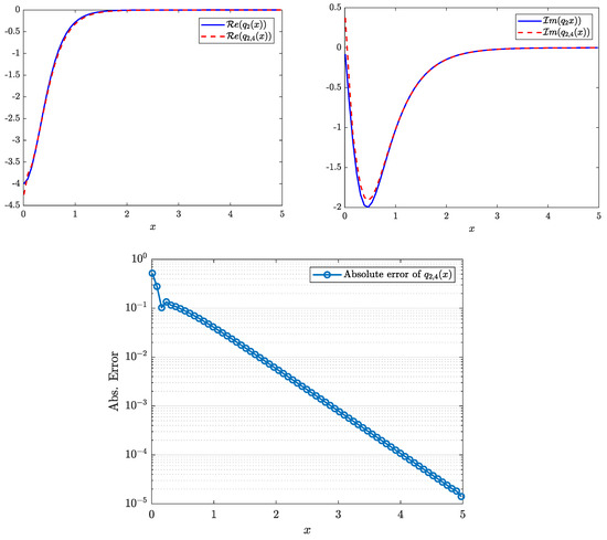
Consider the scattering function $s_2\left(\rho \right)$ and denote the noisy scattering function by ${\widehat{s}}_2\left(\rho \right):=s_2\left(\rho \right)+\epsilon \left(\rho \right)$. Here, $\epsilon \left(\rho \right)$ is $\pm 5\%$ uniformly distributed complex-valued noise (the percentage of the noise is applied pointwise to the modulus and argument of the value of $s_2\left(\rho \right)$). The maximum absolute error of ${\widehat{s}}_2$ on the line ${\mathcal{L}}_{\eta =0.5}$ is $2.46\times {10}^{-1}$. The potential was recovered using five equations with a maximum absolute error of $5.2\times {10}^{-1}$. The real and imaginary parts of the potential and the absolute error of its recovery are shown in Figure 19.

Figure 19. Example 17: figures on the top part show the recovered potential $q_{2,4}\left(x\right)$, and the bottom figure shows the absolute error of the recovered potential.

Despite the noise that ${\widehat{s}}_2\left(\rho \right)$ produces in the matrix of the system (100), the method recovers the shape of the potential $q_2$ with reasonable accuracy.

Example 18. 

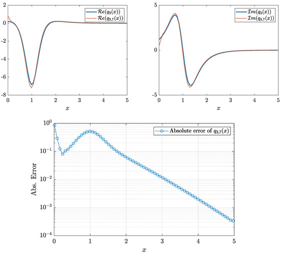
Consider the scattering function $s_3\left(\rho \right)$ and define ${\widehat{s}}_3\left(\rho \right):=s_3\left(\rho \right)+\epsilon \left(\rho \right)$ where $\epsilon \left(\rho \right)$ is a $\pm 10\%$ uniformly distributed complex-valued noise (considered as in the previous example). The maximum absolute error of ${\widehat{s}}_3$ on the line ${\mathcal{L}}_{\eta =0.5}$ is $1.75$. The potential was recovered using eight equations with a maximum absolute error of $8.6\times {10}^{-1}$. The real and imaginary parts of the potential as well as the absolute error of its recovery are shown in Figure 20.

Figure 20. Example 18: figures on the top part show the potential $q_{3,7}\left(x\right)$ recovered with eight equations, and the bottom figure presents the absolute error of the recovered potential.

Although, in this case, the absolute error of ${\widehat{s}}_3\left(\rho \right)$ is larger, the shape of the recovered potential is still quite close to that of the exact one.

5.2.3. In-Out

In this subsection, we consider the results obtained in Section 5.1 as input data for the inverse problem.

Example 19. 

We use the approximate scattering function $s_3\left(\rho \right)$ from Example 10 calculated by (107). Particularly, the form in which it is given allows for us to approximate functions ${\tilde{f}}_{m,c}\left(x\right)$ and ${\tilde{A}}_{mn,c}\left(x\right)$ with the aid of the numerical calculus of residues, i.e., the first procedure in Remark 11 (see Table 19 and Table 20).

Table 19. Example 19: maximum absolute error of the approximation of the function $f_{m,c}\left(x\right)$ using calculus of residues.

m	0	1	2	3
${\displaystyle \underset{x\in (0,15)}{max}\left|f_{m,c}\left(x\right)-{\tilde{f}}_{m,c}\left(x\right)\right|}$	$4.795\times {10}^{-10}$	$1.911\times {10}^{-10}$	$7.494\times {10}^{-11}$	$2.861\times {10}^{-11}$

Table 20. Example 19: maximum absolute error of the approximation of the function $A_{mn,c}\left(x\right)$ using calculus of residues.

m	${\displaystyle \underset{\mathit{x}\in (0,15)}{max}\left|{\mathit{A}}_{\mathit{mn},\mathit{c}}\left(\mathit{x}\right)-{\tilde{\mathit{A}}}_{\mathit{mn},\mathit{c}}\left(\mathit{x}\right)\right|}$
	$\mathit{n}=\mathbf{0}$	$\mathit{n}=\mathbf{1}$	$\mathit{n}=\mathbf{2}$	$\mathit{n}=\mathbf{3}$
0	$2.995\times {10}^{-10}$	$1.206\times {10}^{-10}$	$4.835\times {10}^{-11}$	$1.895\times {10}^{-11}$
1	$1.206\times {10}^{-10}$	$4.835\times {10}^{-11}$	$1.895\times {10}^{-11}$	$7.238\times {10}^{-12}$
2	$4.835\times {10}^{-11}$	$1.895\times {10}^{-11}$	$7.238\times {10}^{-12}$	$2.73\times {10}^{-12}$
3	$1.895\times {10}^{-11}$	$7.238\times {10}^{-12}$	$2.73\times {10}^{-12}$	$1.057\times {10}^{-12}$

The potential $q_3\left(x\right)$ was recovered with an absolute error of $1.8\times {10}^{-5}$ in the interval $(0,15)$ using 8 equations.

Example 20. 

Consider the approximate scattering function $s_1\left(\rho \right)$ from Example 11. The coefficient $a_0\left(x\right)$ was recovered using 14 equations with a maximum absolute error of $4.29\times {10}^{-3}$, from which the potential was recovered with a maximum absolute error of $0.23$, Figure 21.

Figure 21. The (left) figure shows the recovered potential $q_{1,13}\left(x\right)$, and the (right) figure presents the absolute error of the recovered potential.

Example 21. 

Consider the approximate scattering data obtained in Example 9. The approximate functions ${\tilde{f}}_m\left(x\right)$ (see Table 21) and ${\tilde{A}}_{mn}\left(x\right)$ (see Table 22) were obtained accurately enough to recover the potential (see Table 23).

Table 21. Example 21: maximum absolute error of the approximation of the function $f_m\left(x\right)$.

m	0	1	2	3
${\displaystyle \underset{x\in (0,100)}{max}\left|f_m\left(x\right)-{\tilde{f}}_m\left(x\right)\right|}$	$8.92\times {10}^{-3}$	$2.97\times {10}^{-3}$	$9.91\times {10}^{-4}$	$3.3\times {10}^{-4}$

Table 22. Example 21: maximum absolute error of the approximation of the function $A_{mn}\left(x\right)$.

m	${\displaystyle \underset{\mathit{x}\in (0,15)}{max}\left|{\mathit{A}}_{\mathit{mn}}\left(\mathit{x}\right)-{\tilde{\mathit{A}}}_{\mathit{mn}}\left(\mathit{x}\right)\right|}$
	$\mathit{n}=\mathbf{0}$	$\mathit{n}=\mathbf{1}$	$\mathit{n}=\mathbf{2}$	$\mathit{n}=\mathbf{3}$
0	$1.5\times {10}^{-7}$	$4.8\times {10}^{-8}$	$1.6\times {10}^{-8}$	$5.4\times {10}^{-9}$
1	$2.7\times {10}^{-6}$	$1.6\times {10}^{-8}$	$5.4\times {10}^{-9}$	$1.8\times {10}^{-9}$
2	$9\times {10}^{-6}$	$2.9\times {10}^{-6}$	$1.8\times {10}^{-9}$	$6\times {10}^{-10}$
3	$3\times {10}^{-6}$	$9.9\times {10}^{-7}$	$3.3\times {10}^{-7}$	$2\times {10}^{-10}$

Table 23. Maximum absolute error of the approximation of the potential by the recovered potential $q_{2,M}\left(x\right)$.

M in (100)	${\displaystyle \underset{\mathit{x}\in (0,20)}{max}\left|{\mathit{q}}_2\left(\mathit{x}\right)-{\mathit{q}}_{2_{\mathit{M}}}\left(\mathit{x}\right)\right|}$
0	$1.09$
1	$1.63\times {10}^{-1}$
2	$6.44\times {10}^{-2}$
3	$5.41\times {10}^{-2}$
5	$5.3\times {10}^{-2}$
7	$5.3\times {10}^{-2}$

Figure 22 illustrates the stability and convergence of the method with the absolute error stabilized at $5.3\times {10}^{-2}$.

Figure 22. Absolute error of the approximation of the potential by the recovered potential $q_{2,M}\left(x\right)$ using $1,2,3,4,6$ and 8 equations.

Example 22. 

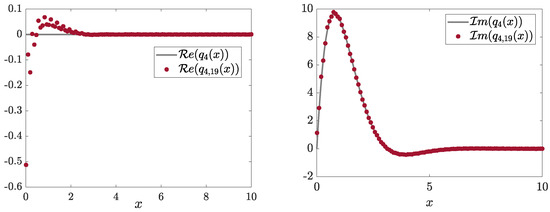
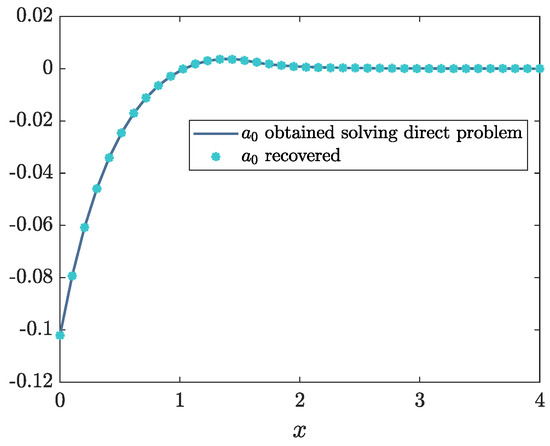
Consider the potential $q_4\left(x\right)=30isin\left(x\right)exp(-x)$ introduced in Example 12. Using the results of the solution of the direct scattering problem from Example 12, we recover $q_4\left(x\right)$ using 20 equations with a maximum absolute error of $8.67\times {10}^{-1}$ (Figure 23).

Figure 23. Real (left) and imaginary (right) parts of the exact potential and the recovered $q_{4,19}\left(x\right)$ ($R=30$).

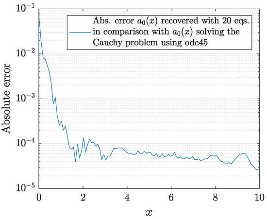
It is worth mentioning that the coefficient $a_0\left(x\right)$ is recovered with an absolute error of $2.28\times {10}^{-2}$ (Figure 24). The error is calculated and compared with the solution of the Cauchy problem

$$\begin{array}{cc}\hfill a_0^{″}\left(x\right)& -a_0^{{}_{{}^{\prime }}}\left(x\right)=q_4\left(x\right)(a_0\left(x\right)+1),\hfill \\ \hfill a_0\left(b\right)& =0,a_0^{\prime }\left(b\right)=-\frac{1}{2},\hfill \end{array}$$

(109)

for a sufficiently large value of $b>0$, obtained using ode45 routine of Matlab2021a.

Figure 24. Example 22: absolute error of the recovered coefficient $a_0\left(x\right)$ with 20 equations.

This is a case where closed formulas for the scattering data set are unavailable. Therefore, the In–Out procedure confirms a satisfactory accuracy in the solution of both the direct and inverse scattering problems.

Example 23. 

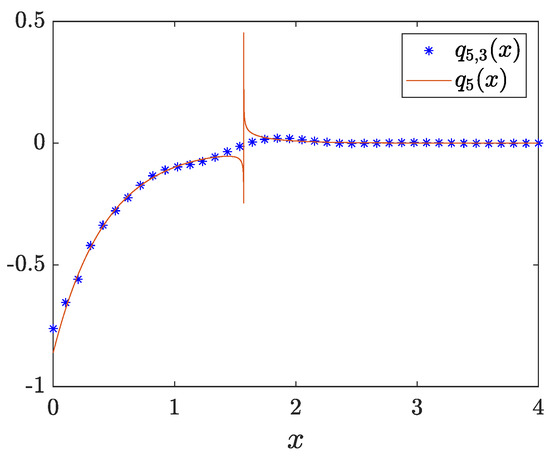
Consider the singular potential

$$q_5\left(x\right)=\frac{exp(-2.5x)}{{\left(x-\frac{\pi }{2}\right)}^{1/3}}.$$

In Table 24, we present the parameter ${\epsilon }_N$ for different values of N in (103).

Table 24. Example 23: indicator ${\epsilon }_N$ for different values of N.

N	${\mathit{\epsilon }}_{\mathit{N}}$ for $\mathit{x}\in [0,4]$	N	${\mathit{\epsilon }}_{\mathit{N}}$ for $\mathit{x}\in [0,4]$
2	$1.57\times {10}^{-1}$	35	$1.10\times {10}^{-3}$
3	$5.24\times {10}^{-2}$	40	$1.03\times {10}^{-3}$
5	$3.97\times {10}^{-3}$	45	$9.57\times {10}^{-4}$
10	$2.25\times {10}^{-3}$	150	$4.84\times {10}^{-4}$
15	$1.77\times {10}^{-3}$	250	$3.60\times {10}^{-4}$
25	$1.33\times {10}^{-3}$	450	$2.56\times {10}^{-4}$

Using data from Table 24, we computed the scattering data with $N=45$. No eigenvalue was detected, so the scattering data set consists of the scattering function approximated by the expression

$$s_5\left(\rho \right)\approx \frac{e_{5,45}(-\rho )}{e_{5,45}\left(\rho \right)},\rho \in \mathbb{R}.$$

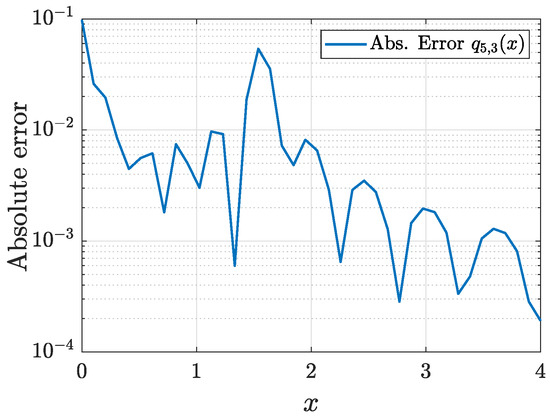
Using this scattering data set to solve the inverse problem, we obtained the coefficient $a_0\left(x\right)$ as shown in Figure 25. The maximum absolute error resulted in $1.9\times {10}^{-4}$.

Figure 25. Example 23: coefficient $a_0\left(x\right)$ with four equations.

The potential is recovered as shown in Figure 26. The corresponding absolute error is presented in Figure 27. Indeed, the maximum absolute error is $9.82\times {10}^{-2}$.

Figure 26. Recovered potential $q_{5,3}\left(x\right)$.

Figure 27. Absolute error of $q_{5,3}\left(x\right)$.

This example shows the applicability of the proposed algorithms to both the solution of the direct and inverse scattering problems in the case of non-smooth potentials.

6. Conclusions

An approach to solving the direct and inverse scattering problems on the half-line for the one-dimensional Schrödinger equation with an exponentially decreasing complex-valued potential is developed. It is based on a series representation of the Jost solution from [25], which is shown in the present work to remain valid in a non-selfadjoining case.

When solving the direct problem, this representation is used to calculate the scattering data set through a simple and efficient procedure, which includes a proposed algorithm for computing normalization polynomials (which are part of the scattering data set) by solving a finite system of linear algebraic equations for its coefficients.

When solving the inverse problem, the use of the series representation combined with the Gel’fand–Levitan equation reduces the problem to a system of linear algebraic equations for the series coefficients, and the knowledge of the first coefficient is sufficient to recover the potential.

The numerical results illustrate the remarkable accuracy of the proposed algorithms in solving both the direct and inverse scattering problems.

References

- Bagarello, F.; Gazeau, J.P.; Szafraniec, F.H.; Znojil, M. Non-Selfadjoint Operators in Quantum Physics; John Wiley & Sons: Hoboken, NJ, USA, 2015. [Google Scholar]
- Bender, C.M.; Boettcher, S. Real spectra in non-Hermitian Hamiltonians having P T symmetry. Phys. Rev. Lett. 1998, 80, 5243. [Google Scholar] [CrossRef]
- Bender, C.M.; Boettcher, S. Quasi-exactly solvable quartic potential. J. Phys. A Math. Gen. 1998, 31, L273. [Google Scholar] [CrossRef]
- Ushveridze, A.G. Quasi-Exactly Solvable Models in Quantum Mechanics; CRC Press: New York, NY, USA, 2017. [Google Scholar]
- Chandrasekhar, S. On characteristic value problems in high order differential equations which arise in studies on hydrodynamic and hydromagnetic stability. Am. Math. 1954, 61, 32–45. [Google Scholar] [CrossRef]
- Dolph, C.L. Recent developments in some non-self-adjoint problems of mathematical physics. Bull. Am. Math. 1961, 67, 1–69. [Google Scholar] [CrossRef]
- Moiseyev, N. Non-Hermitian Quantum Mechanics; Cambridge University Press: Cambridge, UK, 2011. [Google Scholar]
- Lombard, R.J.; Mezhoud, R.; Yekken, R.; Ezzouar, U.B. Complex potentials with real eigenvalues and the inverse problem. Rom. J. Phys. 2018, 63, 101. [Google Scholar]
- Hryniv, O.R.; Manko, S.S. Inverse scattering on the half-line for ZS-AKNS systems with integrable potentials. Integr. Oper. Theory 2016, 84, 323–355. [Google Scholar] [CrossRef]
- Bairamov, E.; Seyyidoglu, M.S. Non-Self-Adjoint singular Sturm-Liouville problems with boundary conditions dependent on the eigenparameter. In Abstract and Applied Analysis; Hindawi: London, UK, 2010; Volume 2010. [Google Scholar]
- Gasymov, M.G. On the decomposition in a series of eigenfunctions for a nonselfconjugate boundary value problem of the solution of a differential equation with a singularity at a zero point. Dokl. Akad. Nauk Russ. Acad. Sci. 1965, 165, 261–264. [Google Scholar]
- Naimark, M.A. Linear Differential Operators. Part II: Linear Differential Operators in Hilbert Space; Dawson, E.R.; Everitt, W.N., Translators; Ungar Publishing: New York, NY, USA, 1968. [Google Scholar]
- Yurko, V.A. Introduction to the Theory of Inverse Spectral Problems; Fizmatlit: Moscow, Russia, 2007. (In Russian) [Google Scholar]
- Barrera-Figueroa, V. Analysis of the spectral singularities of Schrödinger operator with complex potential by means of the SPPS method. J. Phys. Conf. Ser. 2016, 698, 012029. [Google Scholar] [CrossRef]
- Kir, E. Spectrum and principal functions of the non-self-adjoint Sturm–Liouville operators with a singular potential. Appl. Math. 2005, 18, 1247–1255. [Google Scholar] [CrossRef]
- Naimark, M.A. Investigation of the spectrum and the expansion in eigenfunctions of a nonselfadjoint operator of the second order on a semi-axis. Tr. Mosk. Mat. Obs. 1954, 3, 181–270. (In Russian) [Google Scholar]
- Pavlov, B.S. On the non-selfadjoint operator −y″ + q(x)y on a semiaxis. Dokl. Akad. Nauk SSSR 1961, 141, 807–810. (In Russian) [Google Scholar]
- Pavlov, B.S. On a Non-Selfadjoint Schrödinger operator, Probl. Math. Phys., No. I, Spectral Theory and Wave Processes; Izdat. Leningrad. Univ.: Leningrad, Russia, 1966; pp. 102–132. (In Russian) [Google Scholar]
- Pavlov, B.S. On a Non-Selfadjoint Schrödinger Operator II, Problems of Mathematical Physics, No. 2, Spectral Theory, Diffraction Problems; Izdat. Leningrad. Univ: Leningrad, Russia, 1967; pp. 133–157. (In Russian) [Google Scholar]
- Sabatier, P.C. Applied Inverse Problems; Lecture Notes in Physics; Springer: Heidelberg, Germany, 1978; Volume 85. [Google Scholar]
- Samsonov, B.F. Spectral singularities of non-Hermitian Hamiltonians and SUSY transformations. J. Phys. A Math. Gen. 2005, 38, L571. [Google Scholar] [CrossRef]
- Sitenko, A.G. Lectures in Scattering Theory; Pergamon Press: Oxford, UK, 1971. [Google Scholar]
- Agranovich, Z.S.; Marchenko, V.A. The Inverse Problem of Scattering Theory; Courier Dover Publications: New York, NY, USA, 2020. [Google Scholar]
- Freiling, G.; Yurko, V. Inverse Sturm–Liouville Problems and Their Applications; NOVA Science Publishers: New York, NY, USA, 2001. [Google Scholar]
- Kravchenko, V.V. On a method for solving the inverse scattering problem on the line. Math. Methods Appl. Sci. 2019, 42, 1321–1327. [Google Scholar] [CrossRef]
- Kravchenko, V.V. Direct and Inverse Sturm-Liouville Problems: A Method of Solution, Frontiers in Mathematics; Birkhäuser: Cham, Switzerland, 2020. [Google Scholar]
- Delgado, B.B.; Khmelnytskaya, K.V.; Kravchenko, V.V. A representation for Jost solutions and an efficient method for solving the spectral problem on the half line. Math. Methods Appl. Sci. 2020, 43, 9304–9319. [Google Scholar] [CrossRef]
- Baker, G.A., Jr.; Graves-Morris, P.R. Padé Approximants, Part I: Basic Theory; Cambridge University Press: Cambridge, UK, 1981. [Google Scholar]
- Baker, G.A., Jr.; Graves-Morris, P.R. Padé Approximants, Part 2: Extensions and Applications; Cambridge University Press: Cambridge, UK, 1981. [Google Scholar]
- Henrici, P. Applied and Computational Complex Analysis; Power Series, Integration, Conformal Mapping, Location of Zeros; John Wiley & Sons: New York, NY, USA, 1974; Volume 1. [Google Scholar]
- Suetin, S.P. Padé approximants and efficient analytic continuation of a power series. Russ. Math. Surv. 2002, 57, 43. [Google Scholar] [CrossRef]
- Bondarenko, E.I.; Rofe-Beketov, F.S. Inverse scattering problem on the semiaxis for the system with the triangle matrix potential. Zhurnal Mat. Fiz. Anal. Geom. [J. Math. Phys. Anal. Geom.] 2003, 10, 412–424. [Google Scholar]
- Levitan, B.M. Inverse Sturm-Liouville Problems; VSP: Zeist, The Netherlands, 1987. [Google Scholar]
- Lyantse, V.É. The inverse problem for a nonselfadjoint operator. Dokl. Akad. Nauk. Russ. Acad. Sci. 1966, 166, 30–33. [Google Scholar]
- Xu, X.C.; Bondarenko, N.P. Stability of the inverse scattering problem for the self-adjoint matrix Schrödinger operator on the half line. Stud. Appl. Math. 2022, 149, 815–838. [Google Scholar] [CrossRef]
- Delgado, B.B.; Khmelnytskaya, K.V.; Kravchenko, V.V. The transmutation operator method for efficient solution of the inverse Sturm-Liouville problem on a half-line. Math. Methods Appl. Sci. 2019, 42, 7359–7366. [Google Scholar] [CrossRef]
- Grudsky, S.M.; Kravchenko, V.V.; Torba, S.M. Realization of the inverse scattering transform method for the Korteweg-de Vries equation. Math. Methods Appl. Sci. 2023, 46, 9217–9251. [Google Scholar] [CrossRef]
- Kravchenko, V.V.; Shishkina, E.L.; Torba, S.M. A transmutation operator method for solving the inverse quantum scattering problem. Inverse Probl. 2020, 36, 125007. [Google Scholar] [CrossRef]
- Lyantse, V.É. An analog of the inverse problem of scattering theory for a nonselfadjoint operator. Mat. Sb. 1967, 1, 485. (In Russian) [Google Scholar]
- Suetin, P.K. Classical Orthogonal Polynomials, 3rd ed.; Fizmatlit: Moscow, Russia, 2005. (In Russian) [Google Scholar]
- Szego, G. Orthogonal Polynomials, American Mathematical Society Colloquium Publications, 23; American Mathematical Society: New York, NY, USA, 1939. [Google Scholar]
- Xiang, S. Asymptotics on Laguerre or Hermite polynomial expansions and their applications in Gauss quadrature. J. Math. Anal. Appl. 2012, 393, 434–444. [Google Scholar] [CrossRef][Green Version]
- Frank, R.L.; Laptev, A.; Safronov, O. On the number of eigenvalues of Schrödinger operators with complex potentials. J. Lond. Math. Soc. 2016, 94, 377–390. [Google Scholar] [CrossRef][Green Version]
- Brown, B.M.; Langer, M.; Marletta, M.; Tretter, C.; Wagenhofer, M. Eigenvalue bounds for the singular Sturm–Liouville problem with a complex potential. J. Phys. A Math. Gen. 2003, 36, 3773. [Google Scholar] [CrossRef]
- Chanane, B. Computing the spectrum of non-self-adjoint Sturm–Liouville problems with parameter-dependent boundary conditions. J. Comput. Appl. Math. 2007, 206, 229–237. [Google Scholar] [CrossRef]
- Satsuma, J.; Yajima, N.B. Initial value problems of one-dimensional self-modulation of nonlinear waves in dispersive media. Prog. Theor. Phys. Suppl. 1974, 55, 284–306. [Google Scholar] [CrossRef]
- Akhiezer, N.I.; Glazman, I.M. Theory of Linear Operators in Hilbert Space; Dover: New York, NY, USA, 1993. [Google Scholar]
- Gradshteyn, I.S.; Ryzhik, I.M. Table of Integrals, Series, and Products; Academic Press: New York, NY, USA, 2007. [Google Scholar]
- Erdélyi, A.; Magnus, W.; Oberhettinger, F.; Tricomi, F.G. Higher Transcendental Functions; McGraw-Hill Book Co.: New York, NY, USA, 1953; Volume 1. [Google Scholar]
- Ancarani, L.U.; Gasaneo, G. Derivatives of any order of the Gaussian hypergeometric function 2F1(a,b,c;z) with respect to the parameters a, b and c. J. Phys. A Math. Theor. 2009, 42, 395208. [Google Scholar] [CrossRef]
- Ramm, A.G. Inverse Problems: Mathematical and Analytical Techniques with Applications to Engineering; Springer: New York, NY, USA, 2005. [Google Scholar]
- Trefethen, L.N. Approximation Theory and Approximation Practice; SIAM: Philadelphia, PA, USA, 2013. [Google Scholar]
- Trefethen, L.N. Quantifying the ill-conditioning of analytic continuation. BIT Numer. Math. 2020, 60, 901–915. [Google Scholar] [CrossRef]
- Kravchenko, V.V.; Torba, S.M.; Velasco-García, U. Spectral parameter power series for polynomial pencils of Sturm-Liouville operators and Zakharov-Shabat systems. J. Math. Phys. 2015, 56, 073508. [Google Scholar] [CrossRef]
- Roussos, I.M. Improper Riemann Integrals; Taylor & Francis Group: Boca Raton, FL, USA, 2013. [Google Scholar]
- Davis, P.J.; Rabinowitz, P. Methods of Numerical Integration, 2nd ed.; Dover Publishers: New York, NY, USA, 2007. [Google Scholar]
- Kantorovich, L.V.; Akilov, G.P. Functional Analysis, 2nd ed.; Silcock, H.L., Translator; Pergamon Press: Oxford-Elmsford, NY, USA, 1982. [Google Scholar]
- Mikhlin, S.G. The Numerical Performance of Variational Methods; Wolters-Noordhoff Publishing: Groningen, The Netherlands, 1971. [Google Scholar]
- D’Errico, J. SLM-Shape Language Modeling. 2009. Available online: http://www.mathworks.commatlabcentral/fileexchange/24443-slm-shape-language-modeling:Mathworks (accessed on 10 March 2022).
- Sarnari, A.J.; Živanović, R. Robust Padé approximation for the holomorphic embedding load flow. In Proceedings of the 2016 Australasian Universities Power Engineering Conference (AUPEC), Brisbane, Australia, 25–28 September 2016; pp. 1–6. [Google Scholar]
- Ibryaeva, O.L.; Aduko, V.M. An algorithm for computing a Padé approximant with minimal degree denominator. J. Comput. Appl. Math. 2013, 237, 529–541. [Google Scholar] [CrossRef]
- Ibryaeva, O.L. A new algorithm for computing Padé approximants and its implementation in Matlab. Bull. South Ural. State Univ. Ser. Math. Model. Program. 2011, 10, 99–107. (In Russian) [Google Scholar]
Disclaimer/Publisher’s Note: The statements, opinions and data contained in all publications are solely those of the individual author(s) and contributor(s) and not of MDPI and/or the editor(s). MDPI and/or the editor(s) disclaim responsibility for any injury to people or property resulting from any ideas, methods, instructions or products referred to in the content. |
© 2023 by the authors. Licensee MDPI, Basel, Switzerland. This article is an open access article distributed under the terms and conditions of the Creative Commons Attribution (CC BY) license (https://creativecommons.org/licenses/by/4.0/).