3D Simulation of Debris Flows with the Coupled Eulerian–Lagrangian Method and an Investigation of the Runout

Abstract

In landslide risk management, it is important to estimate the run-out distance of landslides (or debris flows) such that the consequences can be estimated. This research presents an innovative array of dimensionless equations that effectively estimate run-out distances, supported by both experimental data and numerical simulations. We employ the coupled Eulerian–Lagrangian (CEL) method to confront the challenges presented in large deformations during landslides. The soil is modelled using the Mohr–Coulomb model, and the failure of cohesionless soil slopes (e.g., sand slopes) is studied. The simulation results are used to study the characteristics of flows and run-out distances. We suggest a normalized run-out and introduce new scaling relationships for it under different conditions such as different plane angles and material properties. The granular flows under different scales can be compared directly with this new scaling law. The new relationships are validated by both experimental and numerical data. Our analysis reveals that the normalized run-out distance in debris flows is contingent on the initial geometry, plane angle, and material properties. An increase in debris volume and plane angle can contribute to an increase in the normalized run-out distance, while a rise in friction angles causes a decrease. In the case of landslides, the normalized run-out distance depends on material properties and the slope angle. An increase in slope angle leads to a corresponding increase in the normalized run-out distance.

1. Introduction

Granular flows (e.g., rock and debris avalanches) are one of the most common landslides in mountainous areas. They often have the characteristics of high speed and long run-out distance, which seriously threaten the safety of lives and property both upstream and downstream [1,2]. Granular flows happened in Sichuan, China in 2017 caused a large number of casualties and property damage [3,4,5,6,7]. The run-out distance of landslides was more than 2600 m within only 60 s and finally blocked a 1200-m stretch of the Songping Stream and a 1600-m stretch of the road. Severe disasters can be avoided if the run-out distance of the granular flow is estimated reasonably.

Lube et al. [8] and Lajeunesse et al. [9] studied the collapse of cylindrical sand columns on the horizontal plane. Experiments have shown that the granular flow mechanism and the final deposition are greatly affected by the initial aspect ratio. The mechanism and the final deposition of the granular flows are different with different aspect ratios. To find the mechanisms of the various collapse and determine the key factors of the empirical equations (such as the critical aspect ratio), a large number of experiments were conducted under different conditions [10,11,12,13,14]. These studies have generally understood the overall process of granular flow from initiation and given a feasible empirical equation. However, these equations did not consider the influence of the mass or volume on the run-out distance, so columns with different scales are hard to directly compare. Therefore, it is necessary to propose a generalized new empirical equation that is not affected by the geometric size.

In addition to the initial aspect ratio, material properties show great effect on granular flows. Lube et al. [8,15] studied the column collapse of different materials, including rice, sugar, and coarse sand, and suggested that the internal friction angles of materials cannot affect the final deposition of the column. On the contrary, some studies using other materials indicate that the internal friction angles have a significant impact on the final deposition and run-out distance [9,16].

Compared with the experiments, numerical methods are better at controlling the material properties and can complement the limitation of experiments. Many numerical methods can well predict the extent of the landslides. For example, simulations of column collapse and landslides have been conducted using the discrete elements method (DEM) [14,17,18] and smoothed particle hydrodynamics (SPH) [12,19,20,21]. DEM can accurately describe problems at the particle scale, so it is theoretically suitable for granular flows. However, when involved with millions of particles, such as simulations of 3D cases, the demand for computing resources is quite large, which is a huge challenge even for high-performance clusters. However, 3D simulations are necessary because the granular flow in the 2D cannot capture the flow in the width direction. As an alternative tool, the coupled Euler–Lagrange (CEL) method is used in this paper to handle both the failure of sensitive clay and granular materials. The CEL method retains the advantages of the Euler and Lagrange methods and can accurately simulate the large deformation landslide problem [22,23,24,25]. Lin et al. [26] studied the interaction between granular flows and the structure, which shows the power of the CEL method to simulate granular problems.

In this paper, coupling of the empirical equation and the CEL method is adopted to access the run-out distance of landslides. The CEL method is used to simulate the entire process of column collapse and capture the run-out distance. A new generalized empirical equation including geometric size was proposed to consider the influence of the geometric structure in granular flows. Two new classes of scaling laws are proposed and extended to 3D situations. Results are in good agreement with the experimental data in the literature, which demonstrates the accuracy of the newly proposed scaling law and empirical equations.

2. Methodology

2.1. Coupled Eulerian–Lagrangian (CEL) Method

In this study, the coupled Eulerian–Lagrangian (CEL) method is used for all simulations. The CEL method was first proposed by Noh [27] with the aim of harnessing the benefits and circumventing the drawbacks of both Lagrangian and Eulerian methods. The entire computational domain was partitioned into several subdomains using Lagrangian and Eulerian descriptions, respectively. Coupled calculations were performed after coordinating the physical quantities within these subdomains, which is the foundation for the CEL method. A wide range of new CEL methods have been proposed [28,29]. The current CEL method uses a fixed Eulerian mesh, allowing materials like soil to move freely, which avoids mesh distortion problems. The CEL method uses the operator splitting method. The nodes move together with materials in a Lagrangian step and then map back to the fixed Eulerian mesh [30] in the second step. This method is based on the explicit integration scheme. As a commonly used large deformation modelling method, CEL has been coupled into the commercial software Abaqus [31]. All the simulations in this study are based on the CEL method in Abaqus.

2.1.1. Governing Equations

Lagrangian description focuses on the process of a material flowing through time and space and can give its time-varying motion path. Eulerian description focuses on representing materials flowing through a particular spatial location at different times. In continuum mechanics, material derivative describes the changing time rate of a material affected by the velocity field. It can be used as a concatenation of Lagrangian and Eulerian descriptions:

$$\frac{D\zeta }{Dt}=\frac{\partial \zeta }{\partial t}+\mathit{v}·\nabla \zeta$$

(1)

where $\zeta$ and $\mathit{v}$ are an arbitrary field variable and the material velocity, respectively. $D\zeta /Dt$ is the material time derivative and $\partial \zeta /\partial t$ is the spatial time derivative. $\mathit{v}·\nabla \zeta$ is the convective term.

The mass and momentum equations are

$$\frac{D\rho }{Dt}+\rho \nabla ·\mathit{v}=0$$

(2)

$$\rho \frac{D\mathit{v}}{Dt}=\nabla ·\mathit{\sigma }+\rho \mathbf{b}$$

(3)

where $\rho$ is the material density, $\mathit{\sigma }$ is the Cauchy stress tensor, $\mathbf{b}$ is the body force. Eulerian conservation equations are obtained by substituting Equation (1) into Equations (2) and (3):

$$\frac{\partial \rho }{\partial t}+\nabla \left(\rho \mathit{v}\right)=0$$

(4)

$$\frac{\partial \rho \mathit{v}}{\partial t}+\nabla ·\left(\rho \mathit{v}⨂\mathit{v}\right)=\nabla ·\mathit{\sigma }+\rho \mathbf{b}.$$

(5)

2.1.2. Operator Splitting

A common form of Eulerian governing equations is

$$\frac{\partial \zeta }{\partial t}+\nabla \mathit{\Phi }=\mathit{S}$$

(6)

where $\mathit{\Phi }$ is the flux function and $\mathit{S}$ is the source term. Equation (6) can be divided into two equations by operator splitting:

$$\frac{\partial \zeta }{\partial t}=\mathit{S}$$

(7)

$$\frac{\partial \zeta }{\partial t}+\nabla \mathit{\Phi }=0.$$

(8)

Equation (7) is the Lagrangian step and (8) is the Eulerian step with the convective term. Figure 1 shows the Eulerian formula, remapping the deformed mesh to the initial fixed mesh and calculating the volume of material that is transferred between adjacent elements. Then adjust the Lagrangian solution variable to consider the material flow between adjacent elements through the transport algorithm.

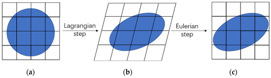
Figure 1. Illustration of two steps in the coupled Eulerian–Lagrangian method. (a) Initial mesh. (b) Deformed mesh. (c) Remapping to the initial mesh.

2.1.3. Lagrangian and Eulerian Steps Based on Explicit Integration Scheme

The virtual work equation is based on the momentum conservation equation:

$${\int }_{\mathrm{v}}p\mathit{a}·\delta \mathit{u}d\mathrm{v}+{\int }_{\mathrm{v}}\mathit{\sigma }:\delta \mathit{\epsilon }d\mathrm{v}={\int }_s\mathit{t}·\delta \mathit{u}ds+{\int }_{\mathrm{v}}p\mathit{b}·\delta \mathit{u}d\mathrm{v}$$

(9)

where $\delta \mathit{\epsilon }$ and $\delta \mathit{u}$ are the virtual strain and displacement, respectively. $\mathit{a}$ is the spatial acceleration and $\mathit{t}$ is the traction. Since the current configuration in the Eulerian step is used rather than the initial configuration, an updated Lagrangian formula is applied in the Lagrangian step. The discrete equation is

$$\mathit{M}\mathit{a}+{\mathit{F}}^{int}={\mathit{F}}^{ext}$$

(10)

where $\mathit{M}$ is the diagonal lumped mass matrix. ${\mathit{F}}^{int}$ are the internal force vectors and ${\mathit{F}}^{ext}$ are the external force vectors.

An explicit formula uses the central difference method to advance the solution in time:

$${\mathit{a}}^n={\mathit{M}}^{-1}({\mathit{F}}^{ext}-{\mathit{F}}^{int})$$

(11)

$${\mathbf{v}}^{n+1/2}={\mathbf{v}}^{n-1/2}+\Delta t{\mathit{a}}^n$$

(12)

$${\mathit{x}}^{n+1}={\mathit{x}}^n+\Delta t{\mathbf{v}}^{n+1/2}$$

(13)

The Eulerian step must deal with more than one material, and empty elements are filled with the void material. Elements in Eulerian method are mixed elements in which all material interfaces exist. Due to the relative motion between the deformed and initially fixed mesh, the Eulerian step calculates the transport between adjacent elements. The explicit time step is used, where a material point can only cross in one element in a single step. The transport calculation in the Eulerian step can be divided into several one-dimensional steps. For the structured meshes, the one-dimensional sweeps go along the direction of the mesh edges, while for unstructured meshes, the sweep is performed in the coordinate direction [32].

2.1.4. General Contact Based on the Penalty Method

The contact in the CEL method between Eulerian and Lagrangian parts is discretized using the general contact method, which is related to the penalty contact method. The penalty contact method is less stringent compared to the kinematic contact method. Seeds are created on the Lagrangian element edges and faces while anchor points are created on the Eulerian material surface. The penalty method is similar to the spring deformation. Figure 2 shows the contact using penalty methods.

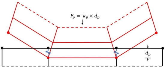
Figure 2. Illustration of the contact based on the penalty method.

$F_p$ represents the contact force and is enforced between anchor points and seeds. $d_p$ represents the penetration distance. The relationship is expressed as below:

$$F_p=k_p\times d_p$$

(14)

where the factor $k_p$ is the penalty stiffness that is related to the material parameters.

2.2. Mohr–Coulomb Model

The Mohr–Coulomb model is widely used in geotechnical engineering. This theory assumes that yield occurs when the shear stress at any point within the soil reaches a value that is linearly dependent on the normal stress in the same plane. The theory relies on a set of Mohr’s circles to calculate the yield stress. The yield line is tangent to all Mohr’s circles. The equation of the yield line is expressed as

$$\tau =c-\sigma \mathrm{t}\mathrm{a}\mathrm{n}\phi$$

(15)

where $\tau$ is the shear stress, $\sigma$ is the normal stress and is negative in compression. $c$ is the cohesion of the material and $\phi$ is the friction angle. It is noted that when the friction angle equals zero, the Mohr–Coulomb material can be considered equivalent to a Tresca material.

Figure 3 shows the Mohr–Coulomb model on the meridional plane and deviatoric plane, respectively. $R$ represents the radius of Mohr’s circle.

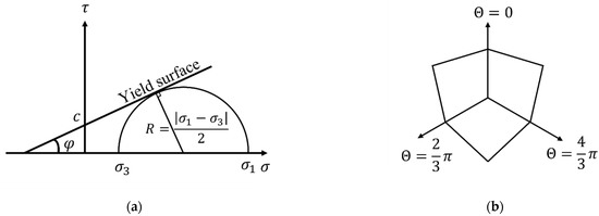
Figure 3. Mohr–Coulomb model. (a) Mohr–Coulomb model on the meridional plane. (b) Mohr–Coulomb model on the deviatoric plane.

Form Figure 3:

$${\tau }_{max}=R\mathrm{c}\mathrm{o}\mathrm{s}\phi .$$

(16)

The yield function can be written in terms of three stress invariants for general stress states as

$$F=R_{mc}q-p\mathrm{t}\mathrm{a}\mathrm{n}\phi -c=0$$

(17)

$$R_{mc}\left(\mathsf{\Theta },\phi \right)=\frac{1}{\sqrt{3}\mathrm{c}\mathrm{o}\mathrm{s}\phi }\mathrm{s}\mathrm{i}\mathrm{n}\left(\mathsf{\Theta }+\frac{\pi }{3}\right)+\frac{1}{3}\mathrm{c}\mathrm{o}\mathrm{s}\left(\mathsf{\Theta }+\frac{\pi }{3}\right)\mathrm{t}\mathrm{a}\mathrm{n}\phi =0$$

(18)

where $\mathsf{\Theta }$ is the deviatoric polar angle and is defined as

$$\mathrm{c}\mathrm{o}\mathrm{s}3\mathsf{\Theta }={\left(\frac{J_3}{\sqrt{3J_2}}\right)}^3.$$

(19)

where $J_2$ and $J_3$ are the second and third invariant of deviatoric stress, respectively.

To avoid the gradient discontinuities occurred at the tip of the model in the associated flow rule, a hyperbolic function is used as the Mohr–Coulomb flow potential function in the meridional stress plane and the smooth elliptic function is chosen in the deviatoric stress plane [33]:

$$G=\sqrt{{\left(ϵc_0\mathrm{t}\mathrm{a}\mathrm{n}\psi \right)}^2+{\left(R_{mw}q\right)}^2}-p\mathrm{t}\mathrm{a}\mathrm{n}\psi$$

(20)

$$R_{mw}\left(\mathsf{\Theta },e\right)=\frac{4\left(1-e^2\right){\mathrm{c}\mathrm{o}\mathrm{s}}^2\mathsf{\Theta }+{\left(2e-1\right)}^2}{2\left(1-e^2\right)\mathrm{c}\mathrm{o}\mathrm{s}\mathsf{\Theta }+\left(2e-1\right)\sqrt{4\left(1-e^2\right){\mathrm{c}\mathrm{o}\mathrm{s}}^2\mathsf{\Theta }+5e^2-4e}}{R}_{mc}\left(\frac{\pi }{3},\phi \right)$$

(21)

$$R_{mc}\left(\frac{\pi }{3},\phi \right)=\frac{3-\mathrm{s}\mathrm{i}\mathrm{n}\phi }{6\mathrm{c}\mathrm{o}\mathrm{s}\phi }$$

(22)

where $\psi$ is the dilation angle. $ϵ$, the default value of 0.1, is the meridional eccentricity which determines the degree to which the hyperbolic function is close to the original Mohr–Coulomb model on the meridional plane (the proximity of the solid black line and the dashed red line in the Figure 4a). $c_0$ is the initial cohesion yield stress. $e$ is the deviatoric eccentricity which describes the “out-of-roundedness” on the deviatoric plane and $e=\frac{3-\mathrm{s}\mathrm{i}\mathrm{n}\phi }{3+\mathrm{s}\mathrm{i}\mathrm{n}\phi }$.

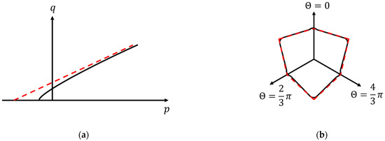
Figure 4. Modified Mohr–Coulomb model in Abaqus. (a) The hyperbolic function on the meridional plane. (b) The elliptic function on the deviatoric plane.

Figure 4 illustrates the hyperbolic function on the meridional plane and the elliptic function on the deviatoric plane, which is used in Abaqus and can be referred to as the modified Mohr–Coulomb model [31]. Red dashed lines represent the original Mohr–Coulomb yield surface and black solid lines represent the approximate yield surface.

3. Collapse of Sand Columns: Two Different Mechanisms

Experimental results suggest that granular flows are largely dependent on the initial aspect ratio $a$ ($a=H_0/L_0$), where $H_0$ and $L_0$ denote the initial height and length of the column in Figure 5a [8,9,15,34]. According to the values of aspect ratio $a$, granular flows can be categorized into two types: debris flows (large aspect ratio) and landslides (small aspect ratio). The studies of these two types of column collapse are conducted using the coupled Eulerian–Lagrangian (CEL) method. The Mohr–Coulomb model is adopted in this section due to the ease of parameter access and its clearly defined physical interpretation.

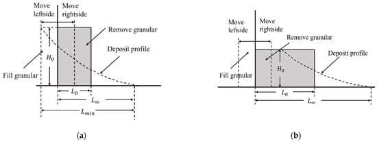
Figure 5. Geometry of the granular column collapse on the horizontal plane. (a) Column with a relatively high aspect ratio. (b) Column with a relatively low aspect ratio.

The collapse processes of granular materials depend on the aspect ratio [8,15,16]. Grey rectangles represent the granular columns and the solid black lines in the left and bottom are the wall and ground in Figure 5. Figure 5a shows a column with a relatively high aspect ratio while Figure 5b presents a column with a low aspect ratio. Two situations are shown in Figure 5 with dashed lines: (1) some materials are removed, and the wall is moved rightward; (2) the wall is moved leftward, and sand particles are filled into the void areas. The collapse is affected in Figure 5a because the intersection of the deposit profile to the left boundary changes. In Figure 5b, moving the left wall has no effect because the intersection on the top surface is not changed. The collapse depends on the initial column geometry, not only the height but also the width. So, the aspect ratio is defined to describe the collapse as $a=H_0/L_0$.

When the top of the deposit profile coincides with the upper left corner of the rectangle, moving the wall further to the leftward will not affect the collapse. Therefore, the $L_{min}$ can be defined (as shown in Figure 5a), and a minimum aspect ratio is $a_{min}=H_0/L_{min}$. Once the aspect ratio $a$ is smaller than $a_{min}$, the length will not affect the collapse. The tall column can be defined as the aspect ratio larger than $a_{min}$, while the shallow column is defined when the aspect ratio is smaller than $a_{min}$. We examine the collapse of tall columns (e.g., debris flows) in Section 4 and shallow columns (e.g., landsldies) in Section 5.

4. Collapse of Tall Columns

4.1. Features of Flow

Column collapse with a high aspect ratio is like long run-out debris flows. Figure 6 shows the collapse of tall column simulated using the CEL method ($L_0=0.05 \mathrm{m}$ and $H_0=0.25 \mathrm{m}$). Soil with a mean density of 2.1 g/cm³ and friction angle of 21.9° is used for the granular material with no dilatancy. Mesh size in CEL simulations is chosen as one-tenth of the square root of the initial cross-sectional area ($\frac{\sqrt{S_0}}{10}$).

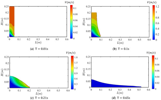
Figure 6. Collapse of the tall column ($a=5$).

In Figure 6, only sand particles above a fracture surface (soil with color other than blue) flow in the early stage, as shown in Figure 6a. This surface intersects the left side boundary to generate an almost straight line. When the flow continues, the top of this line rises on the left side of the boundary, and fewer sand particles are unstable and participate in the movement (Figure 6b–d). For this collapse, the top of this line remains on the left vertical wall in the entire flow process (Figure 6). Therefore, in terms of tall columns, the final deposit height differs from the initial height. One important characteristic is the evolution of the dynamic interface, which divides the stable and flowing areas. Usually, this interface can be an almost straight line from the bottom corner to the left boundary. By comparing these interfaces at different times (Figure 6), the flow region decreases quickly, and this interface moves to the free surface. The granular flow stops once this interface is consistent with the free surface.

4.2. Deposition Profile and Run-Out

When the granular materials slowly pile up on the horizontal planes, a heap will be formed. The angle of repose (AOR), defined as the angle between the horizontal surface and the free surface of the material heap, is often related to the friction angle of granular materials. The AOR should be transferred to friction angles in the Mohr–Coulomb model for simulations. The deposit in the simulation is better satisfied with collapse experiments of the granular materials when $\mathrm{s}\mathrm{i}\mathrm{n}\phi =\mathrm{t}\mathrm{a}\mathrm{n}AOR$ [19]. Table 1 presents the relationship between the AOR and the $\phi$ used in simulations.

Table 1. Relationship between AOR and $\phi$.

$\mathit{\phi }$ in the Simulations (°)	$\mathbf{atan} \mathbf{\left(}\mathbf{s}\mathbf{i}\mathbf{n}\mathit{\phi }\mathbf{\right)}$ (°)	AOR in the Experiments (°)
21.9	20.4	——
27.0	24.4	24.5 $\pm$ 2.0
36.5	30.7	30.5
40.0	32.7	33.0 $\pm$ 1.0
47.0	36.2	36.5 $\pm$ 4.5

Figure 7 shows the final deposit profiles of tall columns with various aspect ratios. This figure includes CEL and experiment results from Lube et al. [15]. According to Figure 5a and Figure 6, when the aspect ratio grows, the flowing areas above the stable areas also increase. Therefore, the run-out distance will increase. CEL results agree well with the data from experiments. With the growth of the initial aspect ratio, the height and the run-out distance of the final deposit profile grow and show a similar tendency. Considering the characteristics of the continuous method, it is difficult for the CEL method to accurately describe the deposition front, which is made of a small number of sand particles, so the final profile of the front is slightly larger than the experiments, but the overall prediction results maintain a high accuracy.

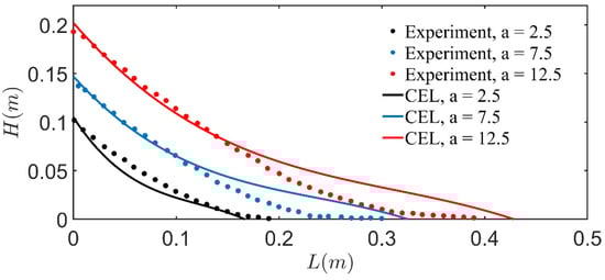
Figure 7. Collapse on horizontal planes with different aspect ratios ($L=0.04 \mathrm{m}$) and experiments data [15]. (Reprinted/adapted with permission from Ref. [15] 2023, American Physical Society).

The empirical equations between dimensionless run-out distance and aspect ratio are defined in the literature as the form of $\left(L_{\mathrm{\infty }}-L_0\right)/L_0={\lambda }_{1}a$ for the shallow column and $(L_{\mathrm{\infty }}-L_0)/L_0={\lambda }_2{a}^b$ for tall columns with $b\approx 0.6$ [9,15,16]. Critical values $a$ for distinguishing tall and shallow columns fluctuate around 1.7 and other parameters can be found in the literature [8,9,15,34].

Considering the collapse of a tall column, adding more sand particles will lead to a larger run-out distance. This is partly because of the mass increase in flowing granular materials. However, if the particles are filled in the $L_0$ direction, which means the aspect ratio $a$ decreases, the dimensionless run-out distance decreases according to the empirical equation. In addition, an extreme case is considered: a shallow column with a very large volume, and a tall column with a very small volume. Obviously, the shallow column will flow a larger absolute run-out distance than the tall column, while the general tendency is that the higher the column is, the longer the run-out distance is. Therefore, when comparing the run-out in different conditions, dimensionless parameters should be used to avoid the influence of the column mass or volume. A new dimensionless run-out distance is proposed as $L_{\mathrm{\infty }}/\sqrt{S_{\mathrm{\infty }}}$, where $S_{\mathrm{\infty }}$ represents the final deposit cross-sectional area [19].

For a given granular column, the only influence factor of the normalized run-out $L_{\mathrm{\infty }}/\sqrt{S_{\mathrm{\infty }}}$ is the aspect ratio, which is the initial dimensionless geometrical parameter of the column. Columns with the same aspect ratio should have the same normalized deposit profiles with a unity cross-sectional area, while the $L_0$ and $H_0$ can differ. As the cross-sectional area in every step of flow is almost the same as the final deposit in experiments, $\sqrt{S_{\mathrm{\infty }}}$ can be considered as the constant value ($\sqrt{S_{\mathrm{\infty }}}=\sqrt{S_0}=\sqrt{H_0{L}_0}$) and it will not influence the CEL simulations. The closer the aspect ratio is to $a_{min}$, the closer the deposit profile is to a statically deposited heap and the closer the deposition front angle is to the AOR. With the increase in aspect ratio, columns collapse more severely and the normalized run-out $L_{\mathrm{\infty }}/\sqrt{S_{\mathrm{\infty }}}$ also increases.

In traditional studies of landslides, researchers usually focus on the flow of the front and the shape of the deposition. It is hard to describe the flow and deposition mechanisms quantitatively. Recently, studies about granular materials collapsing on the horizontal plane have been carried out using laboratory experiments and the discrete element method (DEM) [9,14,34]. Figure 8 shows the relationship between $L_{\mathrm{\infty }}/\sqrt{S_{\mathrm{\infty }}}$ and $a$. This figure contains part of the experimental and DEM data from the literature, and the CEL simulation results in this study. All the data are presented using $L_{\mathrm{\infty }}/\sqrt{S_{\mathrm{\infty }}}$. Since the run-out distance relies on the frictional parameters of the material, a new scaling law is proposed below:

$$\frac{L_{\infty }}{\sqrt{S_{\infty }}}=f_c\left(a,\phi \right)={\lambda }_3\left(\phi \right)-\frac{{\lambda }_4\left(\phi \right)}{\sqrt{a}}$$

(23)

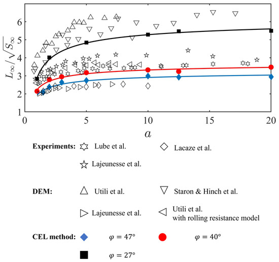
Figure 8. Experiment, DEM data, and fitting curve with the relationship between aspect ratio and run-out distance [9,13,14,15,34]. (Reprinted/adapted with permission from Ref. [9] 2023, AIP Publishing; Ref. [13] 2023, Cambridge University Press; Ref. [14] 2023, Elsevier; Ref. [15] 2023, American Physical Society; Ref. [34] 2023, AIP Publishing).

The run-out distance of the granular column increases with the initial aspect ratio for the given material. However, the normalized run-out distance generally reaches a critical value while the aspect ratio is quite large. In Figure 8, data from the literature are concentrated in three banded regions with the same trend, which is because of the different friction angles of various materials in experiments. The friction angles in experiments cannot be accurately controlled at 27, 40, and 47°. Therefore, there is a difference between the experimental results and the numerical simulation results. The three colored solid lines represent the fitting curve from CEL simulations and have the same tendency as the experimental and DEM data.

4.3. Collapse of Tall Columns on Inclined Planes

Most granular column collapses are conducted on the horizontal planes and two shapes of columns are considered: (1) cylinder column collapse in axisymmetric situations, and (2) wall-bounded rectangular column collapse [8,10]. However, it is also necessary to study the mechanism of flowing on the inclined plane below the AOR of granular columns, for example, what happens when the angle of inclined plane increases and how reliable the equation from horizontal planes is used on inclined planes.

Figure 9 illustrates a column collapse with granular materials on the inclined plane. A rectangular granular column is first placed on the horizontal plane of the same length. The grey rectangular shape is the initial granular column and collapses to the right. The angle between the horizontal and the inclined plane is defined as ${\alpha }_p$. The AOR of granular material is 33.0° $\pm$ 1.0° and has been shown in Table 1. The maximum run-out distance of the column is defined as $L_{\mathrm{\infty }}$.

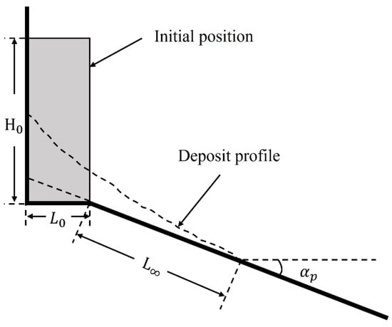
Figure 9. Geometry of granular column collapse on the inclined plane.

Column collapse on the inclined plane is similar to that on the horizontal plane. However, with the increase in the inclined plane angle ${\alpha }_p$, the collapses become generally faster, and the run-out distance becomes larger. The final height of the deposit profile decreases and looks thinner. In Figure 10, three deposit profiles with a constant $a=7$ and the inclined plane angles different from 4.2° to 15° illustrate the characteristic mentioned above.

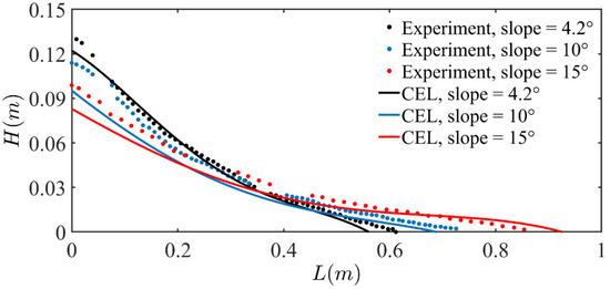
Figure 10. Collapse ($a=7$) on inclined planes and experiments data [10]. (Reprinted/adapted with permission from Ref. [10] 2023, Cambridge University Press).

In Figure 10, the three colorful dotted lines represent the experimental data from Lube et al. [10] and the colorful solid lines are the simulated deposit profiles from CEL simulations. CEL simulations show good agreement with the experiments in terms of most of the deposit profiles and run-out distance. However, the height of the final deposit profiles is slightly lower than the experimental results. In CEL simulations, the left constraint is represented by a frictionless roller boundary condition, while in the experiments, the contact between the left wall and columns is rough. Therefore, the height of the final deposit profile can be different.

Figure 11 illustrates the relationship between $L_{\mathrm{\infty }}/\sqrt{S_{\mathrm{\infty }}}$ and $a$. This figure includes part of experimental data from the Lube et al. [10] and CEL simulation results in this study. All the data are presented using the new dimensionless run-out distance $L_{\mathrm{\infty }}/\sqrt{S_{\mathrm{\infty }}}$. The run-out distance depends on the friction angles $\phi$ and the inclined plane angles ${\alpha }_p$, and Section 4.2 can be considered as the case of ${\alpha }_p=0$. Therefore, empirical Equation (23) is modified as below:

$$\frac{L_{\infty }}{\sqrt{S_{\infty }}}=f_c\left(a,\phi ,{\alpha }_p\right)={\lambda }_3\left({\phi , \alpha }_p\right)-\frac{{\lambda }_4\left(\phi ,{\alpha }_p\right)}{\sqrt{a}}$$

(24)

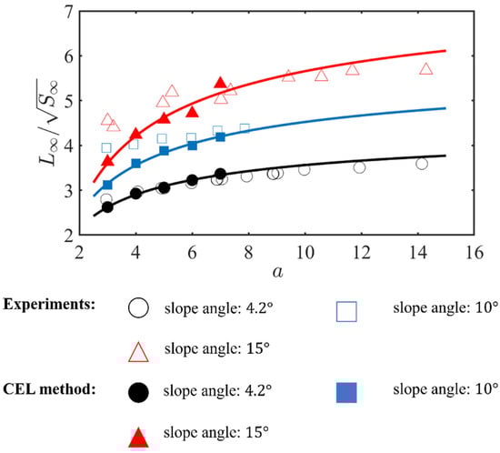
Figure 11. Experiments [10] and CEL results. (Reprinted/adapted with permission from Ref. [10] 2023, Cambridge University Press).

The three colored solid lines represent the dimensionless run-out distance from CEL simulations. The run-out distance of granular columns increases with the inclined plane angle ${\alpha }_p$ for a given material and generally reaches a critical value while the aspect ratio $a$ is large enough.

Figure 12 and Table 2 show the trends and values of ${\lambda }_3$ and ${\lambda }_4$ for various $\phi$ and ${\alpha }_p$ from CEL simulations. $\lambda$ is jointly affected by the friction angle and plane angle, and roughly presents a binary linear relationship. Therefore, two empirical equations are proposed to estimate the values of $\lambda$ in different conditions:

$${\lambda }_3\left({\phi , \alpha }_p\right)=10.52-0.16\times \phi +0.25\times {\alpha }_p$$

(25)

$${\lambda }_4\left({\phi , \alpha }_p\right)=6.33-0.11\times \phi +0.38\times {\alpha }_p.$$

(26)

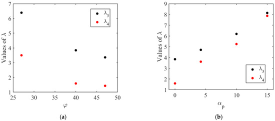
Figure 12. Parameters in the dimensionless equations (fit from CEL simulation Data). (a) Relationship between parameters and friction angles. (b) Relationship between parameters and plane angles.

Table 2. Parameters in the dimensionless equations.

$\mathit{\phi }$ (°)	${\mathit{\alpha }}_{\mathit{p}}$ (°)	${\mathit{\lambda }}_3$	${\mathit{\lambda }}_4$
27	0	6.39	3.50
40		3.84	1.59
47		3.36	1.43
40	4.2	4.71	3.61
	10	6.19	5.25
	15	8.14	7.87

Figure 13 compares the ${\lambda }_3$ and ${\lambda }_4$ in different approaches. Calculated $\lambda$ in the horizontal axis represents parameters directly fitted from the numerical simulation results, while predicted $\lambda$ in the vertical axis represents parameters obtained from empirical Equations (25) and (26). Coefficient of determination ($R^2$) is a statistical measure that represents the proportion of the variance in the dependent variable that can be explained by the independent variable(s) included in the model. Figure 13a,b provide the coefficient of determination for ${\lambda }_3$ and ${\lambda }_4$ with $R_{{\lambda }_3}^2=0.960$ and $R_{{\lambda }_4}^2=0.983$, respectively. This shows that calculated $\lambda$ and predicted $\lambda$ have a very high degree of fit and reflect the accuracy of empirical Equations (25) and (26).

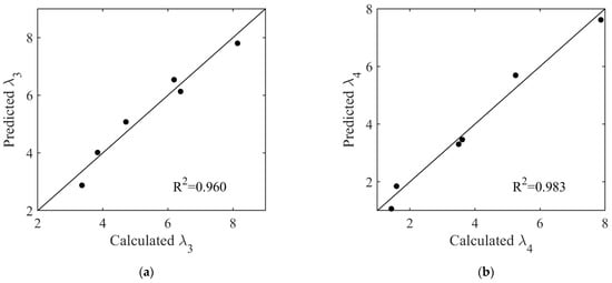
Figure 13. Comparison of parameters $\lambda$ directly obtained from the numerical simulations and fitted empirical equations. (a) comparison of ${\lambda }_3$ from direct calculations and Equations (25). (b) comparison of ${\lambda }_4$ from direct calculations and Equations (26).

4.4. Axisymmetric Collapse of Tall Cylinders

The objective of this section is to model the collapse of granular cylinders on the horizontal plane. Due to the axisymmetric nature, simulations can be simplified to a quarter of cylinder collapse. Experiments were conducted by Lube et al. [8].

Figure 14 illustrates the initial geometry of cylinders with the top and horizontal view, respectively. $L_0$ represents the radius of the cylinder. Solid lines with black color at the bottom represent base planes. The rectangle and sector with grey color are the granular cylinder from the front and top views. Arrow lines are the symmetrical axis of the cylinder and dashed lines are the final deposit profiles of the cylinder. Soil with a mean density of 2.6 g/cm³ is used and AOR is 30.5° as shown in Table 1. The maximum flow distance of the cylinder is defined as $L_{\mathrm{\infty }}$. Mesh size in CEL simulations is chosen as one-tenth of the square root of the initial volume ($\frac{\sqrt[3]{V}}{10}$).

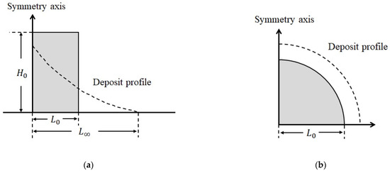
Figure 14. Geometry of unhindered axisymmetric granular flows of cylinders. (a) Vertical cross-section. (b) Horizontal cross-section.

Figure 15 shows the process of unhindered axisymmetric tall cylinder ($a=3$) collapse from the front (Figure 15a–d) and top views (Figure 15e–h). Firstly, only particles on the fracture surface flow at the beginning and the surface of the cylinder has the maximum velocity, as shown in Figure 15a,e. When the flow continues, the top of this dynamic interface goes up on the left boundary (Figure 15b–d,f–h) and less material upon the surface flows until it coincides with the free surface. For this collapse, the top of this dynamic interface moves on the left symmetrical axis in the entire flow process, which is similar to the conclusion of $a>1.7$ in 2D situations. Thus, the final deposit height is inconsistent with the initial height for tall cylinders.

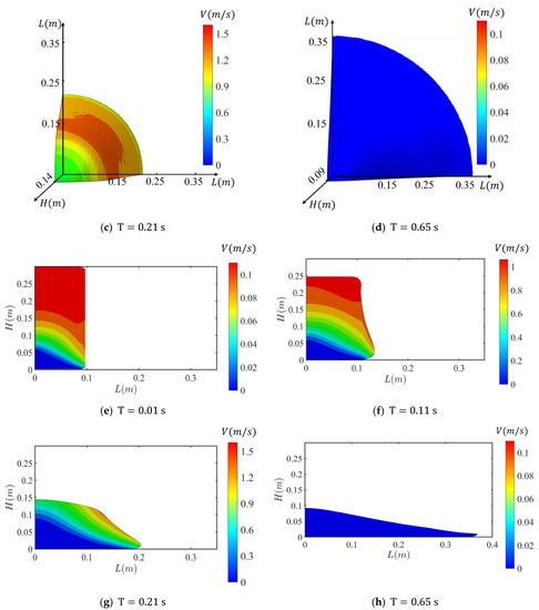
Figure 15. Unhindered axisymmetric tall cylinder ($a=3$) collapse of cylinders.

Figure 16 presents the final deposit profiles of tall cylinders collapse on horizontal planes from the front views using the CEL method. Three different aspect ratios are used in the CEL simulations as $a=2$, $4$, and $6$. The three colored solid lines represent the final deposit profile from CEL simulations. With the increase in aspect ratio, the final height decreases while the final run-out distance grows. Additionally, the cylinders will have similar final deposit profiles with the increase of aspect ratio, which is consistent with the 2D case.

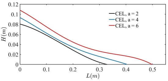
Figure 16. Final deposit profiles of unhindered axisymmetric tall cylinder collapse on horizontal planes.

For cylinder collapse, the influence of mass and volume also need to be avoided. Therefore, a new dimensionless run-out distance $L_{\mathrm{\infty }}/\sqrt[3]{V}$ is proposed for the new empirical equation. According to the literature, the critical value of the aspect ratio is $a\approx 1.7$ [8,9]. Various aspect ratios are considered from 2 to 10 using the CEL method and the run-out distance are compared with the experimental data in Figure 17.

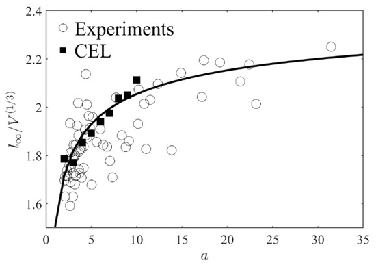
Figure 17. Experimental data [8] and CEL simulation results.

Figure 17 presents part of the data from experiments [8] and CEL simulation results and all the data are normalized using $L_{\mathrm{\infty }}/\sqrt[3]{V}$. The solid black line represents the fitting curve from CEL simulations. The run-out distance of granular cylinders increases with the initial aspect ratios and finally reaches a critical value while the aspect ratio is large enough. Since the run-out relies on the frictional parameters of the material, a new scaling law is proposed below:

$$\frac{L_{\infty }}{\sqrt[3]{V}}=f_c\left(a\right)=2.74-\frac{1.42}{\sqrt[3]{a}}$$

(27)

5. Shallow Columns and Cut Slopes

Granular flows with low aspect ratios (Figure 5b) are similar to landslides. Some two-dimensional experiments were conducted with aluminum rods collapsing on the horizontal planes [12]. The diameters of the aluminum rods are 1.6 or 3.0 mm, and the bulk density is 2.65 g/cm³. The initial friction angle is 21.9°, which is measured in the biaxial tests. These material parameters were used in the CEL simulations. Figure 18a–d shows the process of shallow column collapse using the CEL method ($L_0=0.2 \mathrm{m}$ and $H_0=0.1 \mathrm{m}$). Mesh size in CEL simulations is chosen as one-tenth of the square root of the initial height ($\frac{H_0}{10}$).

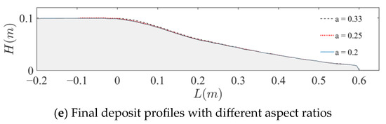
Figure 18. Shallow column collapse.

Figure 18a–d sequentially illustrates the process of the granular flow. Initially, only particles above the fracture surface are observed to flow in the early stage, as shown in Figure 18a. This surface intersects with the top boundary to form an almost straight line, marking a distinct difference from the tall columns in Figure 6a. As the flow continues, this line gradually transitions towards the free surface of the deposit profile, and fewer particles are unstable and flow away (Figure 18b,c). For this kind of collapse, the fracture surface cannot reach the left vertical wall in the entire flow process (Figure 18d). Consequently, in terms of shallow columns, the height of the final deposit profile is essentially equivalent to the initial geometry.

Figure 18e shows three final deposit profiles with different aspect ratios. The grey block represents the cross-section of the collapse. Three colored lines represent the free surface of the final depositions. For ease of comparison, the different deposit profiles are aligned on the right front. It can be clearly observed that columns with different aspect ratios have the same final deposit profiles. Therefore, aspect ratios will not affect the normalized run-out distance of the shallow columns, which validates the assumption in Figure 5b. In this situation, another geometry of columns, slope angles $\beta$, can affect the run-out distance. As shown in Figure 19, the grey trapezoid represents the granular column, and the solid black lines are the boundaries of the slope. Dashed lines denote that the length of the left side extends infinitely, which means the aspect ratio is small enough.

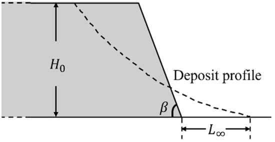
Figure 19. The geometry of sandpile collapses on the horizontal plane.

5.1. Landslides with Different Slope Angles and Friction Angles

Since the columns of various aspect ratios exhibit similarity when their slope angles are the same. Therefore, the height of the column is a constant value in this study. The objective of this section is to simulate the collapse of shallow granular columns on the horizontal plane and analyze the relationship between the run-out distance and slope angles as well as friction angles. Simulations were performed using the Mohr–Coulomb model, while the cohesion was kept at a constant value of 0.

Figure 20 shows the final deposit profiles of shallow column collapse on horizontal planes using the CEL method. The slope angle of the shallow column is the fixed value of $\beta =$ 60° in Figure 20a, and four different friction angles $\phi$ from 21.9° to 47° were used in simulations. The dashed line represents the initial column profile. With the increase in friction angles, the static area on the top left corner expands and the final run-out distance decreases. In addition, all the final profiles seem to intersect at roughly the same point. Figure 20b shows the run-out distance associated with the different slope angles $\beta$ from 40° to 80°, while the friction angle is the constant value of $\phi =$ 21.9°. It is noted that the shallow column keeps static with a slope angle of $\beta =$ 24°, which is close to the friction angle (the dashed line in Figure 20b). When the slope angle decreases, the run-out distance also decreases until the column stays static.

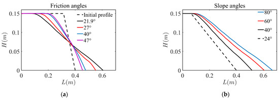
Figure 20. Collapse on horizontal planes with (a) different friction angles (slope angle is 60°) and (b) different slope angles (friction angle is 21.9°).

Since the length of the column is infinity, the normalized run-out $L_{\mathrm{\infty }}/\sqrt{S_{\mathrm{\infty }}}$ is not suitable. A new normalized run-out, $L_{\mathrm{\infty }}/H_0$, is proposed here, where $L_{\mathrm{\infty }}$ is the run-out distance, as shown in Figure 19.

Figure 21 shows the relationship between $L_{\mathrm{\infty }}/H_0$ and $\beta /\phi$. A new scaling law is proposed as below:

$$\frac{L_{\infty }}{H_0}=-1.72\times e^{\left(1-\frac{\beta }{\phi }\right)}+1.59$$

(28)

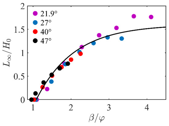
Figure 21. CEL results and fitted relationship between normalized slope angle and run-out distance $L_{\mathrm{\infty }}/H_0$.

In this figure, four different colors represent four different friction angles from 21.9° to 47°. The solid black line represents the fitting curve from CEL simulations. The run-out distance of the granular column increases with the normalized slope angles and finally stops when the slope angle reaches 90°. Slope angles over 90° are not reasonable in nature and thus are not considered in this study. In addition, the run-out distance tends to decrease with the increase in friction angles. Columns tend to be static when the slope angles gradually reach the friction angles.

5.2. Axisymmetric Collapse of Roundtables with Different Slope Angles and Friction Angles

In this section, shallow roundtable collapses with roundtable shapes on the horizontal plane under the action of gravity are simulated using the CEL method. Due to the axisymmetric distribution of roundtables, simulations can be simplified to a quarter of roundtable roundtables collapse.

Figure 22 shows the initial geometry of the unhindered axisymmetric landslides from the front and top views, respectively. The solid black line at the bottom represents the base plane. The trapezoid and sector with grey color are the cross-section of the landslides, which collapses to the right. Arrow lines represent the symmetrical axis of the roundtable, and dashed lines represent the final deposit profile of the roundtable. Soil with a mean density of 2 g/cm³ is used as the material parameter and friction angles are shown in Table 1. The slope angle is 80° in each simulation. The maximum flow distance of the roundtable is defined as $L_{\mathrm{\infty }}$ in Figure 22.

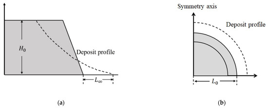
Figure 22. Geometry of unhindered axisymmetric landslides of roundtables. (a) Vertical cross-section. (b) Horizontal cross-section.

Figure 23 shows the process of unhindered axisymmetric landslides collapse from vertical (Figure 23a–d) and horizontal cross-sections (Figure 23e–h). Particles above the fracture surface begin to move away at the beginning. The mobilized soil is concentrated in the upper right corner of the slope while the left side of the slope remains static, as shown in Figure 23a,e. The maximum velocity appears on the front surface. As the collapse progresses, the top and front surfaces progressively merge, forming a new free surface. Fewer particles are instable and participate in the flow (Figure 23b,c,f,g). Finally, the fracture surface coincides with the new free surface and the flow of landslides stops (Figure 23d,h). For landslides, the left side of the slope always stays static, and the final deposit height is consistent with the initial height.

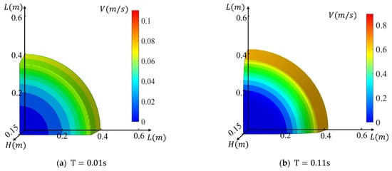
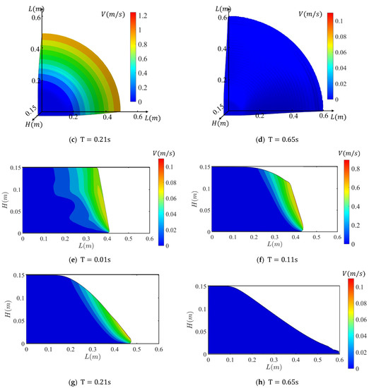
Figure 23. Unhindered axisymmetric landslides of the roundtable.

Figure 24 shows part of the CEL simulation results of the final deposit profiles of unhindered axisymmetric landslides on horizontal planes. The slope angle of the landslides is the fixed value of $\beta =$ 60° in Figure 24a, and four different friction angles $\phi$ from 21.9° to 47° are used in simulations. With the increase in friction angles, the static area on the top left corner grows and the final run-out distance decreases. In addition, all the final profiles intersect almost at the same point. Figure 24b shows the run-out distance between the different slope angles $\beta$ from 40° to 80° with the same friction angle of $\phi =$ 21.9°. The dashed line represents the static roundtable with a slope angle of $\beta =$ 24°, which is close to the friction angle. When the slope angle decreases, the run-out distance also decreases.

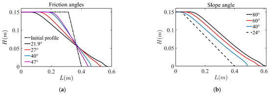
Figure 24. Unhindered axisymmetric landslides of roundtables on horizontal planes with (a) different friction angles (slope angle is 60°) and (b) different slope angles (friction angles is 21.9°).

Figure 25 shows the relationship between $L_{\mathrm{\infty }}/H_0$ and $\beta /\phi$. A new scaling law is proposed as below:

$$\frac{L_{\infty }}{H_0}=-1.52\times e^{\left(1-\frac{\beta }{\phi }\right)}+1.39$$

(29)

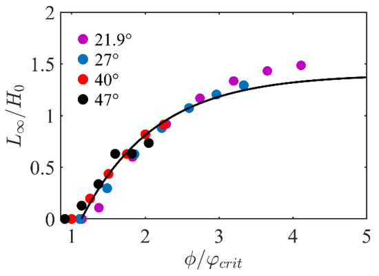
Figure 25. CEL results with fitted relationship between normalized slope angle and run-out distance $L_{\mathrm{\infty }}/H_0$.

Four different colors represent four different friction angles from 21.9° to 47° in Figure 25. The run-out distance of particle roundtables increases with the normalized slope angles and finally stops when the slope angle reaches 90°.

There are some minor discrepancies between the coupled Eulerian–Lagrangian (CEL) simulation results and experimental data, which can be attributed to the limitations of the CEL method. Firstly, the CEL method is based on the finite element method and may not accurately represent the characteristics of discrete granular materials. Secondly, the CEL method cannot effectively handle the change of volume in simulations. However, expansion and contraction behavior are common in granular materials, which relies on the initial state of the material. These behaviors can influence the relationship between the initial and the final cross-sectional area. This study assumes the same cross-sectional area in all simulations: $S_0=S_{\mathrm{\infty }}$. However, laboratory tests [16] indicate a slight difference between the initial and final cross-sectional area: the final cross-sectional area is larger than the initial cross-sectional area by approximately 10%. This discrepancy leads to differences between simulation results and experimental data. Lastly, some experiments indicate that the critical friction coefficient is not a constant value. The coefficient in the inertia state is typically larger than that measured in the quasistatic state [11]. These factors contribute to the slight variations observed between CEL simulations and experimental results.

6. Conclusions

This paper presents the simulations of different kinds of column collapse using the CEL method. The results were validated and compared with different experimental data and DEM simulations.

The run-out distance of cohesionless soil columns is greatly affected by the initial geometry of the columns. Column collapse can be categorized into two types by the critical aspect ratio: tall column collapse as debris flows and shallow column collapse as landslides. In tall column collapse, the aspect ratio is a key factor while in shallow column collapse, slope angle is given primary consideration.

Simulations of the tall columns are divided into three parts: (1) the collapse of the 2D columns on the horizontal plane, (2) the collapse of the 2D columns on the inclined planes with plane angles smaller than the AOR, and (3) the collapse of the 3D cylinders on the horizontal plane. The CEL method completely simulates the entire process of granular column collapse. During the collapse process, a dynamic interface between flow particles and static particles can be observed, and the failure stops when the interface evolves to the granular surface. Various simulations were performed for different initial aspect ratios, and the final deposition was consistent with the experimental results.

To compare column collapse under different scales and obtain general conclusions, a new class of dimensionless run-out distance is proposed to avoid the influence of mass or volume and is extended to 3D situations. A series of empirical equations were established to describe quantitative relationships between the dimensionless run-out distance and the initial aspect ratios in collapse of tall columns. The new scaling law and empirical equations show good results with comparable key features as in experiments and DEM simulations. The results validate the accuracy of this method in simulating both the collapse process and the final deposit profiles under a diverse range of scenarios.

Shallow column collapses, also called landslides, were also performed using CEL simulations. Unlike the flow of tall columns, the collapse of shallow columns is not affected by the initial aspect ratios. CEL simulation shows the same final deposit profile with various aspect ratios. In this situation, run-out distance is affected by the slope angles of columns. Landslides are simulated under different slope and friction angles in 2D and 3D conditions with trapezoidal and roundtable shapes. New scaling laws were proposed for the normalized slope angles. New empirical equations were presented to predict the normalized run-out distance.

References

- Zhao, B.; Su, L.; Wang, Y.; Ji, F.; Li, W.; Tang, C. Insights into the Mobility Characteristics of Seismic Earthflows Related to the Palu and Eastern Iburi Earthquakes. Geomorphology 2021, 391, 107886. [Google Scholar] [CrossRef]
- Guo, X.; Cheng, Q.; Zhang, L.; Zhou, H.; Xing, X.; Li, W.; Wang, Z. Large-Scale in Situ Tests for Shear Strength and Creep Behavior of Moraine Soil at the Dadu River Bridge in Luding, China. Int. J. Geomech. 2022, 22, 04022053. [Google Scholar] [CrossRef]
- Fan, X.; Xu, Q.; Scaringi, G.; Dai, L.; Li, W.; Dong, X.; Zhu, X.; Pei, X.; Dai, K.; Havenith, H.-B. Failure Mechanism and Kinematics of the Deadly June 24th 2017 Xinmo Landslide, Maoxian, Sichuan, China. Landslides 2017, 14, 2129–2146. [Google Scholar] [CrossRef]
- Intrieri, E.; Raspini, F.; Fumagalli, A.; Lu, P.; Del Conte, S.; Farina, P.; Allievi, J.; Ferretti, A.; Casagli, N. The Maoxian Landslide as Seen from Space: Detecting Precursors of Failure with Sentinel-1 Data. Landslides 2018, 15, 123–133. [Google Scholar] [CrossRef]
- Fan, X.; Xu, Q.; Scaringi, G. Brief Communication: Post-Seismic Landslides, the Tough Lesson of a Catastrophe. Nat. Hazards Earth Syst. Sci. 2018, 18, 397–403. [Google Scholar] [CrossRef]
- Dai, K.; Xu, Q.; Li, Z.; Tomás, R.; Fan, X.; Dong, X.; Li, W.; Zhou, Z.; Gou, J.; Ran, P. Post-Disaster Assessment of 2017 Catastrophic Xinmo Landslide (China) by Spaceborne SAR Interferometry. Landslides 2019, 16, 1189–1199. [Google Scholar] [CrossRef]
- Scaringi, G.; Fan, X.; Xu, Q.; Liu, C.; Ouyang, C.; Domènech, G.; Yang, F.; Dai, L. Some Considerations on the Use of Numerical Methods to Simulate Past Landslides and Possible New Failures: The Case of the Recent Xinmo Landslide (Sichuan, China). Landslides 2018, 15, 1359–1375. [Google Scholar] [CrossRef]
- Lube, G.; Huppert, H.E.; Sparks, R.S.J.; Hallworth, M.A. Axisymmetric Collapses of Granular Columns. J. Fluid Mech. 2004, 508, 175–199. [Google Scholar] [CrossRef]
- Lajeunesse, E.; Monnier, J.B.; Homsy, G.M. Granular Slumping on a Horizontal Surface. Phys. Fluids 2005, 17, 103302. [Google Scholar] [CrossRef]
- Lube, G.; Huppert, H.E.; Sparks, R.S.J.; Freundt, A. Granular Column Collapses down Rough, Inclined Channels. J. Fluid Mech. 2011, 675, 347–368. [Google Scholar] [CrossRef]
- Midi, G.D.R. On Dense Granular Flows. Eur. Phys. J. E 2004, 14, 341–365. [Google Scholar] [CrossRef]
- Nguyen, C.T.; Nguyen, C.T.; Bui, H.H.; Nguyen, G.D.; Fukagawa, R. A New SPH-Based Approach to Simulation of Granular Flows Using Viscous Damping and Stress Regularisation. Landslides 2017, 14, 69–81. [Google Scholar] [CrossRef]
- Staron, L.; Hinch, E.J. Study of the Collapse of Granular Columns Using Two-Dimensional Discrete-Grain Simulation. J. Fluid Mech. 2005, 545, 1–27. [Google Scholar] [CrossRef]
- Utili, S.; Zhao, T.; Houlsby, G.T. 3D DEM Investigation of Granular Column Collapse: Evaluation of Debris Motion and Its Destructive Power. Eng. Geol. 2015, 186, 3–16. [Google Scholar] [CrossRef]
- Lube, G.; Huppert, H.E.; Sparks, R.S.J.; Freundt, A. Collapses of Two-Dimensional Granular Columns. Phys. Rev. E Stat. Nonlin. Soft Matter Phys. 2005, 72, 041301. [Google Scholar] [CrossRef]
- Balmforth, N.J.; Kerswell, R.R. Granular Collapse in Two Dimensions. J. Fluid Mech. 2005, 538, 399–428. [Google Scholar] [CrossRef]
- Cundall, P.A.; Strack, O.D. A Discrete Numerical Model for Granular Assemblies. Geotechnique 1979, 29, 47–65. [Google Scholar] [CrossRef]
- Li, X.; Chu, X.; Feng, Y.T. A Discrete Particle Model and Numerical Modeling of the Failure Modes of Granular Materials. Eng. Comput. 2005, 22, 894–920. [Google Scholar] [CrossRef]
- He, X.; Liang, D.; Bolton, M.D. Run-out of Cut-Slope Landslides: Mesh-Free Simulations. Geotechnique 2018, 68, 50–63. [Google Scholar] [CrossRef]
- Bui, H.H.; Fukagawa, R.; Sako, K.; Ohno, S. Lagrangian Meshfree Particles Method (SPH) for Large Deformation and Failure Flows of Geomaterial Using Elastic-Plastic Soil Constitutive Model. Int. J. Numer. Anal. Methods Geomech. 2008, 32, 1537–1570. [Google Scholar] [CrossRef]
- Chen, D.; Huang, W.; Lyamin, A. Finite Particle Method for Static Deformation Problems Solved Using JFNK Method. Comput. Geotech. 2020, 122, 103502. [Google Scholar] [CrossRef]
- Dey, R.; Hawlader, B.; Phillips, R.; Soga, K. Large Deformation Finite-Element Modelling of Progressive Failure Leading to Spread in Sensitive Clay Slopes. Géotechnique 2015, 65, 657–668. [Google Scholar] [CrossRef]
- Xu, H.; He, X.; Sheng, D. Rainfall-Induced Landslides from Initialization to Post-Failure Flows: Stochastic Analysis with Machine Learning. Mathematics 2022, 10, 4426. [Google Scholar] [CrossRef]
- Jeong, S.-S.; Lee, K.-W.; Ko, J.-Y. A Study on the 3D Analysis of Debris Flow Based on Large Deformation Technique (Coupled Eulerian-Lagrangian). J. Korean Geotech. Soc. 2015, 31, 45–57. [Google Scholar] [CrossRef]
- Chen, X.; Zhang, L.; Chen, L.; Li, X.; Liu, D. Slope Stability Analysis Based on the Coupled Eulerian-Lagrangian Finite Element Method. Bull. Eng. Geol. Environ. 2019, 78, 4451–4463. [Google Scholar] [CrossRef]
- Lin, C.-H.; Hung, C.; Hsu, T.-Y. Investigations of Granular Material Behaviors Using Coupled Eulerian-Lagrangian Technique: From Granular Collapse to Fluid-Structure Interaction. Comput. Geotech. 2020, 121, 103485. [Google Scholar] [CrossRef]
- Noh, W.F. CEL: A Time-Dependent, Two-Space-Dimensional, Coupled Euler-Lagrange Code; Lawrence Radiation Laboratory, University of California: Livermore, CA, USA, 1963. [Google Scholar]
- Fedkiw, R.P. Coupling an Eularian Fluid Calculation to a Lagrangian Solid Calculation with the Ghost Fluid Method. J. Comput. Phys. 2002, 175, 200–224. [Google Scholar] [CrossRef]
- Arienti, M.; Hung, P.; Morano, E.; Shepherd, J.E. A Level Set Approach to Eulerian-Lagrangian Coupling. J. Comput. Phys. 2003, 185, 213–251. [Google Scholar] [CrossRef]
- Benson, D.J. Computational Methods in Lagrangian and Eulerian Hydrocodes. Comput. Methods Appl. Mech. Eng. 1992, 99, 235–394. [Google Scholar] [CrossRef]
- Benson, D.J.; Okazawa, S. Contact in a Multi-Material Eulerian Finite Element Formulation. Comput. Methods Appl. Mech. Eng. 2004, 193, 4277–4298. [Google Scholar] [CrossRef]
- Menetrey, P.; Willam, K.J. Triaxial Failure Criterion for Concrete and Its Generalization. Struct. J. 1995, 92, 311–318. [Google Scholar]
- Dassault Systemes. Dassault Systemes ABAQUS 6.14 Documentation; Dassault Systemes Simulia Corporation: Providence, RI, USA, 2014; Volume 651. [Google Scholar]
- Lacaze, L.; Phillips, J.C.; Kerswell, R.R. Planar Collapse of a Granular Column: Experiments and Discrete Element Simulations. Phys. Fluids 2008, 20, 063302. [Google Scholar] [CrossRef]
Disclaimer/Publisher’s Note: The statements, opinions and data contained in all publications are solely those of the individual author(s) and contributor(s) and not of MDPI and/or the editor(s). MDPI and/or the editor(s) disclaim responsibility for any injury to people or property resulting from any ideas, methods, instructions or products referred to in the content. |
© 2023 by the authors. Licensee MDPI, Basel, Switzerland. This article is an open access article distributed under the terms and conditions of the Creative Commons Attribution (CC BY) license (https://creativecommons.org/licenses/by/4.0/).