Dynamics of a Predator–Prey Model with Impulsive Diffusion and Transient/Nontransient Impulsive Harvesting

Abstract

Harvesting is one of the ways for humans to realize economic interests, while unrestricted harvesting will lead to the extinction of populations. This paper proposes a predator–prey model with impulsive diffusion and transient/nontransient impulsive harvesting. In this model, we consider both impulsive harvesting and impulsive diffusion; additionally, predator and prey are harvested simultaneously. First, we obtain the subsystems of the system in prey extinction and predator extinction. We obtain the fixed points of the subsystems by the stroboscopic map theories of impulsive differential equations and analyze their stabilities. Further, we establish the globally asymptotically stable conditions for the prey/predator-extinction periodic solution and the trivial solution of the system, and then the sufficient conditions for the permanence of the system are given. We also perform several numerical simulations to substantiate our results. It is shown that the transient and nontransient impulsive harvesting have strong impacts on the persistence of the predator–prey model.

1. Introduction

In nature, species cannot exist alone; they always interact with other species, such as in competition, predator–prey, or reciprocity. As one of them, the predator–prey relationship is widespread and very important. It is also a main research topic in population dynamics. In the 1940s, Lotka and Volterra proposed the classic predator–prey system. Afterward, the classic predator–prey model has been followed and developed in much literature [1,2,3,4,5,6,7,8], and the study of the dynamics of the predator–prey model has been observed widely in applied mathematics. There are many factors, for example, weather, food supply, mating habits or harvesting, by which the dynamics of the predator–prey population are affected. In [1], Brauer studied the following system:

$$\left\{\begin{array}{c}{\displaystyle x^{\prime }=xf(x,y)-F,}\hfill \\ {\displaystyle y^{\prime }=yg(x,y),}\hfill \end{array}\right.$$

(1)

where prey population $x(t)$ is harvested at a constant time rate F, and f(x,y) and g(x,y) denote the per capita growth rates of prey population $x(t)$ and predator population $y(t)$, respectively. Similar to reference [1], the activities of harvesting are usually assumed to be continuous in formerly published results. Kumar and Kharbanda [2] studied a predator–prey model with nonlinear harvesting. Lv et al. [3] investigated a prey–predator model with continuous harvesting, and the stability of the model is discussed from both local and global perspectives. Although it is preferable from the point of view of both maximizing harvest and sustainability, continuous harvesting is not always realistic, because the harvesting is seasonal or occurs in regular pulses for most species. In [4], a logistic system with impulsive perturbations was investigated. The specific form of the model is as follows:

$$\left\{\begin{array}{c}{\displaystyle x^{\prime }(t)=x(t)(r(t)-a(t)x(t)),t\ne t_k,}\hfill \\ {\displaystyle \Delta x(t)=b_{k}x(t),t=t_k,}\hfill \end{array}\right.$$

(2)

when $b_k<0$, the perturbation means harvesting, $\Delta x(t_k)=x({t_k}^{+})-x(t_k)$. Recently, predator–prey models with impulsive harvesting have been intensively researched. Tian and Gao [5] discussed an instantaneous harvest fishery model. Liu et al. [6] considered a predator–prey model in which predator and prey species are harvested independently with proportion. Wei et al. [7] proposed a ratio-dependent prey–predator model with state-dependent impulsive harvesting. Especially, Jiao [8] mentioned that transient and nontransient pulse harvesting constitute the whole harvesting process in the reality of biological resource management and presented the following model with impulsive effects:

$$\left\{\begin{array}{c}\left.\begin{array}{c}{\displaystyle \frac{d{x}_1(t)}{dt}=-(c_1+d_1)x_1(t),}\hfill \\ {\displaystyle \frac{d{x}_2(t)}{dt}=c_1{x}_1(t)-d_2{x}_2(t),}\hfill \end{array}\right\}t\in (n\tau ,(n+l)\tau ],\hfill \\ \left.\begin{array}{c}\Delta x_1(t)=-u_1{x}_1(t),\hfill \\ \Delta x_2(t)=-u_2{x}_2(t),\hfill \end{array}\right\}t=(n+l)\tau ,\hfill \\ \left.\begin{array}{c}{\displaystyle \frac{d{x}_1(t)}{dt}=-(c_2+d_3)x_1(t)-E_1{x}_1(t),}\hfill \\ {\displaystyle \frac{d{x}_2(t)}{dt}=c_2{x}_1(t)-d_4{x}_2(t)-E_2{x}_2(t),}\hfill \end{array}\right\}t\in ((n+l)\tau ,(n+1)\tau ],\hfill \\ \left.\begin{array}{c}\Delta x_1(t)=x_2(t)(a-b{x}_2(t)),\hfill \\ \Delta x_2(t)=0,\hfill \end{array}\right\}t=(n+1)\tau ,\hfill \end{array}\right.$$

(3)

where the transient impulsive harvesting rate is denoted by $u_i(i=1,2)$ and the nontransient impulsive harvesting coefficient is denoted by $E_i(i=1,2)$. The biological significance of other parameters refer to [5]. In [5,6,7,8], and scholars have studied the persistence and extinction of the investigated predator–prey models. All results show that through proper pulse control, the population will coexist, and then, the purpose of maintaining the balance of the ecosystem can be achieved.

The diffusion of populations is very common in nature and affects the dynamics of the system and the ecological balance. Modern biologists believe that dispersion and migration become necessary for populations due to seasonal changes, lack of food, breeding, or avoidance of predators [9,10,11,12]. Paying attention to species living in patches of the environment, Takeuchi [13] considered the following general single-population system with diffusion:

$$\dot{x_i}=x_i{g}_i(x_i)+\sum _{j=1}^n{D}_{ij}(x_j-x_i),x(0)>0,i=1,2,\dots n,$$

(4)

where $x_i$ is the population density in patch i, $g_i(x_i)$ is the natural growth rate, and $D_{ij}$ is the dispersal rate. Initially, researchers assumed that diffusion between patches was continuous or discrete; however, many species only diffuse over a single period of time in practice. In [14], a model describing the dynamics of single species with impulsive diffusion was given by

$$\left\{\begin{array}{c}\left.\begin{array}{c}{\displaystyle \frac{d{x}_1(t)}{dt}=x_1(t)(a_1-b_1{x}_1(t)),}\hfill \\ {\displaystyle \frac{d{x}_2(t)}{dt}=x_2(t)(a_2-b_2{x}_2(t)),}\hfill \end{array}\right\}t\ne n\tau ,\hfill \\ \left.\begin{array}{c}\Delta x_1(t)=d_1(x_2(t)-x_1(t)),\hfill \\ \Delta x_2(t)=d_2(x_1(t)-x_2(t)),\hfill \end{array}\right\}t=n\tau ,\hfill \end{array}\right.$$

(5)

where $d_i(i=1,2)$ is the dispersal rate in the i-th patch, and the dispersal behavior of species occurs every $\tau$ period. Other examples specific to diffusion models can be seen in [15,16,17]. Cui [15] studied a time-varying logistic population growth model with diffusion. Zhong et al. [16] proposed a fishery model with impulsive diffusion; they assumed that the system consists of two paths connected by diffusion and that the inshore subpopulation is harvested at fixed moments in time. In [17], a predator–prey model assuming diffusion and harvesting occurring at different fixed times was studied by Jiao et al. They considered the case of harvesting both prey and predator populations and performed a dynamic analysis of the model.

Most of the previous research focused only on impulsive harvesting or impulsive diffusion and carried out unilateral harvesting of predators or prey. There still has been no investigation of the predator–prey model with transient/nontransient impulsive harvesting considering both pulse harvesting and diffusion in the literature. In addition, pulse harvesting consists of transient and nontransient impulsive harvesting; predator and prey may also be harvested at the same time. The transient impulsive harvesting process is extremely short, which will cause sudden changes in the population. The nontransient pulse harvesting depends on the current state and will last for a while, which is crucial to the entire process of system development and cannot be ignored in both theoretical analysis and practical application.

2. The Model

Higher-order predators such as tigers are able to create territories. They will not interfere with other areas and only prey in their own territories [18,19,20]. In this paper, we assume predator species are restricted to a single patch, and prey species diffuse between two patches at a fixed moment of time for foraging, breeding, or avoiding predators. From the above point of view and considering transient and nontransient impulsive harvesting exist in populations of both prey and predator, we propose a new predator–prey model with pulse effects, defined as

$$\left\{\begin{array}{c}\left.\begin{array}{c}{\displaystyle \frac{d{x}_1(t)}{dt}=x_1(t)(a_1-b_1{x}_1(t)),}\hfill \\ {\displaystyle \frac{d{x}_2(t)}{dt}=-d_1{x}_2(t)-{\beta }_1{x}_2(t)y(t),}\hfill \\ {\displaystyle \frac{dy(t)}{dt}=y(t)(a_2-b_{2}y(t))+k_1{\beta }_1{x}_2(t)y(t),}\hfill \end{array}\right\}t\in (n\sigma ,(n+\xi )\sigma ],\hfill \\ \left.\begin{array}{c}\Delta x_1(t)=-m_1{x}_1(t),\hfill \\ \Delta x_2(t)=-m_2{x}_2(t),\hfill \\ \Delta y(t)=-m_{3}y(t),\hfill \end{array}\right\}t=(n+\xi )\sigma ,\hfill \\ \left.\begin{array}{c}{\displaystyle \frac{d{x}_1(t)}{dt}=x_1(t)(a_3-b_3{x}_1(t))-h_1{x}_1(t),}\hfill \\ {\displaystyle \frac{d{x}_2(t)}{dt}=-d_2{x}_2(t)-h_2{x}_2(t)-{\beta }_2{x}_2(t)y(t),}\hfill \\ {\displaystyle \frac{dy(t)}{dt}=y(t)(a_4-b_{4}y(t))-h_{3}y(t)+k_2{\beta }_2{x}_2(t)y(t),}\hfill \end{array}\right\}t\in ((n+\xi )\sigma ,(n+1)\sigma ],\hfill \\ \left.\begin{array}{c}\Delta x_1(t)=d(x_2(t)-x_1(t)),\hfill \\ \Delta x_2(t)=d(x_1(t)-x_2(t)),\hfill \\ \Delta y(t)=0,\hfill \end{array}\right\}t=(n+1)\sigma .\hfill \end{array}\right.$$

(6)

where $x_1(t)$ is the population density of prey in patch 1. $x_2(t)$ and $y(t)$ are the population densities of prey and predator in patch 2, respectively. The parameters $a_1,b_1$ denote the intrinsic growth rate and intraspecific competition coefficient of $x_1$, respectively, on $(n\sigma ,(n+\xi )\sigma ]$. $d_1$ is the natural death rate of $x_2$, ${\beta }_1$ is the prey captured rate by y, and $k_1$ is the rate of conversion of nutrients into the reproduction rate of y, on $(n\sigma ,(n+\xi )\sigma ]$. $a_2,b_2$ denote the intrinsic growth rate and intraspecific competition coefficient of y, respectively, on $(n\sigma ,(n+\xi )\sigma ]$. $m_1$, $m_2$, and $m_3$ represent the transient impulsive harvesting rate of $x_1$, $x_2$, and y at time $t=(n+\xi )\sigma$, respectively. $a_3,b_3$ are the intrinsic growth rate and intraspecific competition coefficient of $x_1$, respectively, on $((n+\xi )\sigma ,(n+1)\sigma ]$. $h_1$, $h_2$, and $h_3$ represent the nontransient impulsive harvesting rate of $x_1$, $x_2$, and y, respectively, on $((n+\xi )\sigma ,(n+1)\sigma ]$. $d_2$ is the natural death rate of $x_2$, ${\beta }_2$ is the prey captured rate by y, and $k_2$ represents the rate of conversion of nutrients into the reproduction rate of y on $((n+\xi )\sigma ,(n+1)\sigma ]$. $a_4,b_4$ are the intrinsic growth rate and intraspecific competition coefficients of y, respectively, on $((n+\xi )\sigma ,(n+1)\sigma ]$. $0<d<1$ denotes the dispersal rate of the prey between two patches. $((n+\xi )\sigma ,(n+1)\sigma ]$ is the nontransient impulsive harvesting interval. The pulse diffusion and impulsive harvesting occur every $\sigma$ period. All the parameters are assumed to be positive for biological considerations.

3. Some Lemmas

Denote $U(t)={(x_1(t),x_2(t),y(t))}^T$ as the solution of system (6). It is a piecewise continuous function $U:R_{+}\to R_{+}^3$ and continuous on $(n\sigma ,(n+\xi )\sigma ]\times R_{+}^3$ and $((n+\xi )\sigma ,(n+1)\sigma ]\times R_{+}^3$, respectively, where $R_{+}=[0,\infty )$, $R_{+}^3=\{(x_1,x_2,y):x_1\ge 0,x_2\ge 0,y\ge 0\}$. The global existence and uniqueness of solutions of system $(6)$ is guaranteed by the smoothness properties of $f=(f_1,f_2,f_3)$, which denotes the mapping defined by the right side of system $(6)$ [21].

Lemma 1. 

There exists a constant $M_0>0$ such that $x_1(t)\le M_0$, $x_2(t)\le M_0$, $y(t)\le M_0$ for each solution $(x_1(t),x_2(t),y(t))$ of system $(6)$ with a t large enough.

Proof. 

Define $V(t)=x_1(t)+k{x}_2(t)+y(t)$, and choose $k=max\{k_1,k_2\}$, $d_L=min\{d_1,d_2+h_2\}$. Then, we have

$$\left\{\begin{array}{c}{\displaystyle D^{+}V(t)+d_{L}V(t)=(a_1+d_L)x_1(t)-b_1{x_1}^2(t)-(k-k_1){\beta }_1{x}_2(t)y(t)-k(d_1-d_L)x_2(t)}\hfill \\ {\displaystyle +(a_2+d_L)y(t)-b_2{y}^2(t)\le {\gamma }_1,t\in (n\sigma ,(n+\xi )\sigma ],}\hfill \\ V(t^{+})\le V(t),t=(n+\xi )\sigma ,\hfill \\ {\displaystyle D^{+}V(t)+d_{L}V(t)=[(a_3-h_1)+d_L]x_1(t)-b_3{x_1}^2(t)-(k-k_2){\beta }_2{x}_2(t)y(t)+k{d}_L{x}_2(t)}\hfill \\ -k(d_2+h_2)x_2(t)+[(a_4-h_3)+d_L]y(t)-b_4{y}^2(t)\le {\gamma }_2,t\in ((n+\xi )\sigma ,(n+1)\sigma ],\hfill \\ {\displaystyle V(t^{+})\le (1-d+kd+\frac{d}{k})V(t),t=(n+1)\sigma ,}\hfill \end{array}\right.$$

(7)

here, ${\displaystyle {\gamma }_1=\frac{{(a_1+d_L)}^2}{4b_1}+\frac{{(a_2+d_L)}^2}{4b_2}}$, ${\displaystyle {\gamma }_2=\frac{{[(a_3-h_1)+d_L]}^2}{4b_3}+\frac{{[(a_4-h_3)+d_L]}^2}{4b_4}}$. Take $\gamma =max\{{\gamma }_1,{\gamma }_2\}$, when $t\ne (n+\xi )\sigma$, $t\ne (n+1)\sigma$, we obtain

$$\left\{\begin{array}{c}{\displaystyle D^{+}V(t)+d_{L}V(t)\le \gamma ,}\hfill \\ {\displaystyle V(t^{+})\le (1-d+kd+\frac{d}{k})V(t),t=(n+1)\tau .}\hfill \end{array}\right.$$

(8)

With reference to [11], we obtain

$$\begin{array}{c}{\displaystyle V(t)\le V(0^{+})(1-d+kd+\frac{d}{k})e^{-d_{L}t}+\frac{\gamma }{d_L}(1-d+kd+\frac{d}{k})(1-e^{-d_{L}t})}\hfill \end{array}$$

(9)

      ${\displaystyle \to \frac{\gamma }{d_L}(1-d+kd+\frac{d}{k})}$ as $t\to \infty$.

Hence, $V(t)$ is uniformly ultimately bounded. By the definition of $V(t)$, there exists a constant $M_0>0$ such that $x_1(t)\le M_0$, $x_2(t)\le M_0$, $y(t)\le M_0$ for a t large enough. □

Considering the subsystem of system $(6)$ with $y(t)=0$, we have:

$$\left\{\begin{array}{c}\left.\begin{array}{c}{\displaystyle \frac{d{x}_1(t)}{dt}=x_1(t)(a_1-b_1{x}_1(t)),}\hfill \\ {\displaystyle \frac{d{x}_2(t)}{dt}=-d_1{x}_2(t),}\hfill \end{array}\right\}t\in (n\sigma ,(n+\xi )\sigma ],\hfill \\ \left.\begin{array}{c}\Delta x_1(t)=-m_1{x}_1(t),\hfill \\ \Delta x_2(t)=-m_2{x}_2(t),\hfill \end{array}\right\}t=(n+\xi )\sigma ,\hfill \\ \left.\begin{array}{c}{\displaystyle \frac{d{x}_1(t)}{dt}=x_1(t)(a_3-b_3{x}_1(t))-h_1{x}_1(t),}\hfill \\ {\displaystyle \frac{d{x}_2(t)}{dt}=-d_2{x}_2(t)-h_2{x}_2(t),}\hfill \end{array}\right\}t\in ((n+\xi )\sigma ,(n+1)\sigma ],\hfill \\ \left.\begin{array}{c}\Delta x_1(t)=d(x_2(t)-x_1(t)),\hfill \\ \Delta x_2(t)=d(x_1(t)-x_2(t)),\hfill \end{array}\right\}t=(n+1)\sigma .\hfill \end{array}\right.$$

(10)

By calculation, we obtain the analytic solution of system $(7)$ between pluses:

$$\left\{\begin{array}{c}{x}_1(t)=\left\{\begin{array}{c}{\displaystyle \frac{a_1{e}^{a_1(t-n\sigma )}{x}_1(n{\sigma }^{+})}{a_1+b_1(e^{a_1(t-n\sigma )}-1)x_1(n{\sigma }^{+})},t\in (n\sigma ,(n+\xi )\sigma ],}\hfill \\ {\displaystyle \frac{(a_3-h_1)e^{(a_3-h_1)(t-(n+\xi )\sigma )}{x}_1((n+\xi ){\sigma }^{+})}{(a_3-h_1)+b_3(e^{(a_3-h_1)(t-(n+\xi )\sigma )}-1)x_1((n+\xi ){\sigma }^{+})},}\hfill \\ t\in ((n+\xi )\sigma ,(n+1)\sigma ],\hfill \end{array}\right.\hfill \\ x_2(t)=\left\{\begin{array}{c}{e}^{-d_1(t-n\sigma )}{x}_2(n{\sigma }^{+}),t\in (n\sigma ,(n+\xi )\sigma ],\hfill \\ e^{-(d_2+h_2)(t-(n+\xi )\sigma )}{x}_2((n+\xi ){\sigma }^{+}),t\in ((n+\xi )\sigma ,(n+1)\sigma ],\hfill \end{array}\right.\hfill \end{array}\right.$$

(11)

and the stroboscopic map of system $(10)$:

$$\left\{\begin{array}{c}{\displaystyle x_1((n+1){\sigma }^{+})=\frac{(1-d)AB{x}_1(n{\sigma }^{+})}{B+C{x}_1(n{\sigma }^{+})}+dD{x}_2(n{\sigma }^{+}),}\hfill \\ {\displaystyle x_2((n+1){\sigma }^{+})=\frac{dAB{x}_1(n{\sigma }^{+})}{B+C{x}_1(n{\sigma }^{+})}+(1-d)D{x}_2(n{\sigma }^{+}),}\hfill \end{array}\right.$$

(12)

here, $A=(1-m_1)e^{a_1\xi \sigma +(a_3-h_1)(1-\xi )\sigma }>0,B=a_1(a_3-h_1),C=b_1(a_3-h_1)(e^{a_1\xi \sigma }-1)+a_1{b}_3(1-m_1)e^{a_1\xi \sigma }(e^{(a_3-h_1)(1-\xi )\sigma }-1),0<D=(1-m_2)e^{-d_1\xi \sigma -(d_2+h_2)(1-\xi )\sigma }<1.$ It is easy to see that system $(12)$ has two fixed points $(0,0)$ and $(x_1^{*},x_2^{*})$, where

$$\left\{\begin{array}{c}{\displaystyle x_1^{*}=\frac{B\{(1-d)(A+D)-[1+(1-2d)AD\left]\right\}}{C[1-(1-d)D]},}\hfill \\ {\displaystyle x_2^{*}=\frac{dB\{(1-d)(A+D)-[1+(1-2d)AD\left]\right\}}{C[1-(1-d)D][(1-d)-(1-2d)D]},}\hfill \end{array}\right.$$

(13)

with condition $(1-d)(A+D)>[1+(1-2d)AD]$.

Lemma 2. 

(i) If $(1-d)(A+D)<[1+(1-2d)AD]$ and $(1-2d)AD<1$, the fixed point $(0,0)$ is locally stable,

(ii) If $(1-d)(A+D)>[1+(1-2d)AD]$ and $(1-2d)AD<1$, the positive fixed point $({x_1}^{*},{x_2}^{*})$ is locally stable.

Proof. 

Denote $({x_1}^n,{x_2}^n)=(x_1(n{\sigma }^{+}),x_2(n{\sigma }^{+}))$.

(i) The linearized equation of $(12)$ around $(0,0)$ is

$$\left(\begin{array}{c}{x_1}^{n+1}\hfill \\ {x_2}^{n+1}\hfill \end{array}\right)=M_1\left(\begin{array}{c}{x_1}^n\\ {x_2}^n\end{array}\right),$$

(14)

where

$$M_1=\left(\begin{array}{cc}{\displaystyle (1-d)A}& dD\\ dA& (1-d)D\end{array}\right).$$

(15)

Apparently, the near dynamics of the fixed point $(0,0)$ are determined by linear system $(14)$. The stability of the fixed point $(0,0)$ is determined by the eigenvalues of $M_1$ less than 1. This is true only if $M_1$ satisfies the three Jury conditions [22]:

$$\begin{array}{c}1-det{M}_1>0,\hfill \\ 1+tr{M}_1+det{M}_1>0,\hfill \\ 1-tr{M}_1+det{M}_1>0.\hfill \end{array}.$$

(16)

By $(15)$ and Conditions for $(i)$ in Lemma 2, it is clear that $tr{M}_1=(1-d)A+(1-d)D>0$. Hence, $1+tr{M}_1+det{M}_1>0$ holds, if $1-tr{M}_1+det{M}_1>0$ is true. Calculating

$$\begin{array}{c}{\displaystyle 1-det{M}_1=1-[{(1-d)}^{2}AD-d^{2}AD]=1-(1-2d)AD>0.}\hfill \\ {\displaystyle 1-tr{M}_1+det{M}_1=1-[(1-d)A+(1-d)D]+[{(1-d)}^{2}AD-d^{2}AD]}\hfill \\ {\displaystyle =1+(1-2d)AD)-(1-d)(A+D)>0.}\hfill \end{array}.$$

(17)

Therefore, the fixed point $(0,0)$ is locally stable.

(ii) Similarly, we can study the local stability of positive fixed point $({x_1}^{*},{x_2}^{*})$ by Jury conditions. In the neighborhood of $({x_1}^{*},{x_2}^{*})$, system $(12)$ is controlled by the linearization of

$$\left(\begin{array}{c}{x_1}^{n+1}-{x_1}^{*}\hfill \\ {x_2}^{n+1}-{x_2}^{*}\hfill \end{array}\right)=M_2\left(\begin{array}{c}{x_1}^n-{x_1}^{*}\\ {x_2}^n-{x_2}^{*}\end{array}\right),$$

(18)

where

$$M_2=\left(\begin{array}{cc}{\displaystyle \frac{(1-d)A{B}^2}{{(B+C{x_1}^{*})}^2}}& dD\\ {\displaystyle \frac{dA{B}^2}{{(B+C{x_1}^{*})}^2}}& (1-d)D\end{array}\right).$$

(19)

Obviously, ${\displaystyle tr{M}_2=\frac{(1-d)A{B}^2}{{(B+C{x_1}^{*})}^2}+(1-d)D>0}$. Hence, $1+tr{M}_2+det{M}_2>0$ holds, if $1-t{r}_{2}M+det{M}_2>0$ is true. Calculating

$$\begin{array}{c}{\displaystyle 1-det{M}_2=1-[\frac{{(1-d)}^{2}A{B}^{2}D}{{(B+C{x_1}^{*})}^2}-\frac{d^{2}A{B}^{2}D}{{(B+C{x_1}^{*})}^2}]}\hfill \\ {\displaystyle =1-(1-2d)AD\frac{B^2}{{(B+C{x_1}^{*})}^2}>0.}\hfill \\ {\displaystyle 1-tr{M}_2+det{M}_2=1-[\frac{(1-d)A{B}^2}{{(B+C{x_1}^{*})}^2}+(1-d)D]+[\frac{{(1-d)}^{2}A{B}^{2}D}{{(B+C{x_1}^{*})}^2}-\frac{d^{2}A{B}^{2}D}{{(B+C{x_1}^{*})}^2}]}\hfill \\ {\displaystyle =1-(1-d)D-\frac{A{B}^2[(1-d)+(2d-1)D]}{{(B+C{x_1}^{*})}^2}}\hfill \\ {\displaystyle =\frac{[1-(1-d)D]\{(1-d)(A+D)-[1+(1-2d)AD\left]\right\}}{A[(1-d)-(1-2d)D]}>0.}\hfill \end{array}$$

(20)

Therefore, the positive fixed point $({x_1}^{*},{x_2}^{*})$ is locally stable. □

Lemma 3. 

(i) If $(1-d)(A+D)<[1+(1-2d)AD]$ and $(1-2d)AD<1$, the fixed point $(0,0)$ is globally asymptotically stable,

(ii) If $(1-d)(A+D)>[1+(1-2d)AD]$ and $(1-2d)AD<1$, the positive fixed point $({x_1}^{*},{x_2}^{*})$ is globally asymptotically stable.

Proof. 

In lemma 2, we proved that the two fixed point are locally stable under the corresponding conditions, respectively. Next, we only need to prove the global attractiveness. According to Theorem 2.2 in reference [23], we rewrite system $(12)$ as a map $T:R_{+}^2\to R_{+}^2$:

$$\left\{\begin{array}{c}{\displaystyle T_1(x_1,x_2)=\frac{(1-d)AB{x}_1}{B+C{x}_1}+dD{x}_2,}\hfill \\ {\displaystyle T_2(x_1,x_2)=\frac{dAB{x}_1}{B+C{x}_1}+(1-d)D{x}_2.}\hfill \end{array}\right.$$

(21)

For any $(x_1,x_2)>0$, it is obvious that $T:R_{+}^2\to R_{+}^2$ is continuous, and $C^1$ in $int(R_{+}^2)$ and $T(0,0)=0$. Since

$$DT(x_1,x_2)=\left(\begin{array}{cc}{\displaystyle \frac{\partial T_1}{\partial x_1}}& {\displaystyle \frac{\partial T_1}{\partial x_2}}\\ {\displaystyle \frac{\partial T_2}{\partial x_1}}& {\displaystyle \frac{\partial T_2}{\partial x_2}}\end{array}\right)=\left(\begin{array}{cc}{\displaystyle \frac{(1-d)A{B}^2}{{(B+C{x}_1)}^2}}& dD\\ {\displaystyle \frac{dA{B}^2}{{(B+C{x}_1)}^2}}& (1-d)D\end{array}\right),$$

(22)

then $DT(0,0)=M_1$ and ${lim}_{\begin{array}{c}{x}_i\to 0,x_i>0(i=1,2)\end{array}}DT(x_1,x_2)=DT(0,0)$. Moreover,

$(a)$ $DT(x_1,x_2)>0$ for $(x_1,x_2)>0$,

$(b)$ If $0<(x_1,x_2)<(\widehat{x_1},\widehat{x_2})$, then $DT(\widehat{x_1},\widehat{x_2})\le DT(x_1,x_2)(\not\equiv DT(x_1,x_2))$.

Let ${\lambda }^{*}=\rho (DT(0,0))$; due to $DT(0,0)=M_1$, we have ${\lambda }^{*}<1$ for $(1-d)(A+D)<[1+(1-2d)AD]$, while ${\lambda }^{*}>1$ for $(1-d)(A+D)>[1+(1-2d)AD]$. According to theorem 2.2 in reference [23] and boundedness of solutions, we can see that for any $(x_1,x_2)>0$, if $(1-d)(A+D)<[1+(1-2d)AD]$, then ${lim}_{n\to \infty }{T}^n(x_1,x_2)=(0,0)$, and there is a unique nonzero fixed point $q=(q1,q2)$ of $T(x_1,x_2)$; if $(1-d)(A+D)>[1+(1-2d)AD]$, then ${lim}_{n\to \infty }{T}^n(x_1,x_2)=(q1,q2)$.

From the above discussion, we know that $q=({x_1}^{*},{x_2}^{*})$. Hence, for $(1-d)(A+D)>[1+(1-2d)AD]$ and $(1-2d)AD<1$, system $(12)$ has a unique positive fixed point $({x_1}^{*},{x_2}^{*})$ and it is globally asymptotically stable. □

Similarly to Refs. [8,17], we can obtain the next lemma.

Lemma 4. 

(i) If $(1-d)(A+D)<[1+(1-2d)AD]$ and $(1-2d)AD<1$, the trivial periodic solution $(0,0)$ of system $(10)$ is globally asymptotically stable,

(ii) If $(1-d)(A+D)>[1+(1-2d)AD]$ and $(1-2d)AD<1$, the periodic solution $(\widetilde{x_1(t)},\widetilde{x_2(t)})$ of system $(10)$ is globally asymptotically stable, where

$$\left\{\begin{array}{c}\widetilde{x_1(t)}=\left\{\begin{array}{c}{\displaystyle \frac{a_1{x_1}^{*}{e}^{a_1(t-n\sigma )}}{a_1+b_1{x_1}^{*}(e^{a_1(t-n\sigma )}-1)},t\in (n\sigma ,(n+\xi )\sigma ],}\hfill \\ {\displaystyle \frac{(a_3-h_1){x_1}^{**}{e}^{(a_3-h_1)(t-(n+\xi )\sigma )}}{(a_3-h_1)+b_3{x_1}^{**}(e^{(a_3-h_1)(t-(n+\xi )\sigma )}-1)},t\in ((n+\xi )\sigma ,(n+1)\sigma ],}\hfill \end{array}\right.\hfill \\ \widetilde{x_2(t)}=\left\{\begin{array}{c}{x_2}^{*}{e}^{-d_1(t-n\sigma )},t\in (n\sigma ,(n+\xi )\sigma ],\hfill \\ {x_2}^{**}{e}^{-(d_2+h_2)(t-(n+\xi )\sigma )},t\in ((n+\xi )\sigma ,(n+1)\sigma ],\hfill \end{array}\right.\hfill \end{array}\right.$$

(23)

here, ${x_1}^{*}$, ${x_2}^{*}$ (see $(13)$) and ${x_1}^{**}$, ${x_2}^{**}$ are determined as

$$\left\{\begin{array}{c}{\displaystyle {x_1}^{**}=\frac{(1-{\mathrm{m}}_1)a_1{\mathrm{e}}^{a_1\xi \sigma }{x_1}^{*}}{a_1+b_1{x_1}^{*}\left(e^{a_1\xi \sigma }-1\right)},}\hfill \\ {x_2}^{**}=(1-m_2)e^{-d_1\xi \sigma }{x_2}^{*}.\hfill \end{array}\right.$$

(24)

Considering another subsystem of system $(6)$ with $x_i(t)=0(i=1,2)$, we have

$$\left\{\begin{array}{c}{\displaystyle \frac{dy(t)}{dt}=y(t)(a_2-b_{2}y(t)),t\in (n\sigma ,(n+\xi )\sigma ],}\hfill \\ \Delta y(t)=-m_{3}y(t),t=(n+\xi )\sigma ,\hfill \\ {\displaystyle \frac{dy(t)}{dt}=y(t)(a_4-b_{4}y(t))-h_{3}y(t),t\in ((n+\xi )\sigma ,(n+1)\sigma ],}\hfill \\ \Delta y(t)=0,t=(n+1)\sigma .\hfill \end{array}\right.$$

(25)

By calculation, we obtain the analytic solution of system $(25)$ between pluses:

$$y(t)=\left\{\begin{array}{c}{\displaystyle \frac{a_2{e}^{a_2(t-n\sigma )}z(n{\sigma }^{+})}{a_2+b_2(e^{a_2(t-n\sigma )}-1)z(n{\sigma }^{+})},t\in (n\sigma ,(n+\xi )\sigma ],}\hfill \\ {\displaystyle \frac{(a_4-h_3)e^{(a_4-h_3)(t-(n+\xi )\sigma )}z((n+\xi ){\sigma }^{+})}{(a_4-h_3)+b_4(e^{(a_4-h_3)(t-(n+\xi )\sigma )}-1)z((n+\xi ){\sigma }^{+})},}\hfill \\ t\in ((n+\xi )\sigma ,(n+1)\sigma ],\hfill \end{array}\right.$$

(26)

and the stroboscopic map of system $(25)$:

$$\begin{array}{c}{\displaystyle y((n+1){\sigma }^{+})=\frac{a_2(a_4-h_3)A_{z}y(n{\sigma }^{+})}{a_2(a_4-h_3)+B_{z}y(n{\sigma }^{+})},}\hfill \end{array}$$

(27)

where

$$\begin{array}{c}{\displaystyle A_z=(1-m_3)e^{a_2\xi \sigma +(a_4-h_3)(1-\xi )\sigma }>0,}\hfill \\ B_z=b_2(a_4-h_3)(e^{a_2\xi \sigma }-1)+a_2{b}_4(1-m_3)e^{a_2\xi \sigma }(e^{(a_4-h_3)(1-\xi )\sigma }-1).\hfill \end{array}$$

(28)

Two fixed points of system $(27)$ are obtained as $y^0$ and $y^{*}$, where

$$\begin{array}{c}{\displaystyle y^{*}=\frac{a_2(a_4-h_3)(A_z-1)}{B_z}}\hfill \end{array}$$

(29)

with condition $A_z>1.$

Lemma 5. 

(i) If $A_z<1$, the fixed point $y^0$ is globally asymptotically stable.

(ii) If $A_z>1$, the positive fixed point $y^{*}$ is globally asymptotically stable.

Proof. 

Denote $y_n=y(n{\sigma }^{+})$, then $(27)$ can be written as

$$\begin{array}{c}{\displaystyle F(y_n)=\frac{a_2(a_4-h_3)A_z{y}_n}{a_2(a_4-h_3)+B_z{y}_n},}\hfill \end{array}$$

(30)

then

$$\begin{array}{c}{\displaystyle \frac{dF(y_n)}{d{y}_n}=\frac{{a_2}^2{(a_4-h_3)}^2{A}_z}{{(a_2(a_4-h_3)+B_z{y}_n)}^2}.}\hfill \end{array}$$

(31)

(i) If $A_z<1$, $y^0$ is the unique fixed point of $(27)$,

$$\frac{dF(y_n)}{d{y}_n}{|}_{y_n=0}=\frac{{a_2}^2{(a_4-h_3)}^2{A}_z}{{(a_2(a_4-h_3))}^2}=A_z<1.$$

(32)

Therefore, if $y^0$ is locally stable, then it is globally asymptotically stable.

(ii) If $A_z>1$, $y^0$ is unstable, $y^{*}$ exists, and

$$\frac{dF(y_n)}{d{y}_n}{|}_{y_n=y^{*}}=\frac{{a_2}^2{(a_4-h_3)}^2{A}_z}{(a_2(a_4-h_3))+B_z{y}^{*}{)}^2}=\frac{{a_2}^2{(a_4-h_3)}^2}{{a_2}^2{(a_4-h_3)}^2}{A}_z=\frac{1}{A_z}<1.$$

(33)

Therefore, if $y^{*}$ is locally stable, then it is globally asymptotically stable. □

Similarly to Ref. [24], we can obtain the next lemma.

Lemma 6. 

(i) If $A_z<1$, the trivial periodic solution of system $(25)$ is globally asymptotically stable.

(ii) If $A_z>1$, the periodic solution $\widetilde{y(t)}$ of system $(25)$ is globally asymptotically stable, where

$$\widetilde{y(t)}=\left\{\begin{array}{c}{\displaystyle \frac{a_2{y}^{*}{e}^{a_2(t-n\sigma )}}{a_2+b_2{y}^{*}(e^{a_2(t-n\sigma )}-1)},t\in (n\sigma ,(n+\xi )\sigma ],}\hfill \\ {\displaystyle \frac{(a_4-h_3)y^{**}{e}^{(a_4-h_3)(t-(n+\xi )\sigma )}}{(a_4-h_3)+b_4{y}^{**}(e^{(a_4-h_3)(t-(n+\xi )\sigma )}-1)},t\in ((n+\xi )\sigma ,(n+1)\sigma ],}\hfill \end{array}\right.$$

(34)

and

$${\displaystyle y^{**}=\frac{(1-m_3)a_2{e}^{a_2\xi \sigma }{y}^{*}}{a_2+b_2(e^{a_2\xi \sigma }-1)y^{*}}.}$$

(35)

4. The Dynamics

Firstly, we study the global asymptotic stability of the boundary periodic solutions $(\widetilde{x_1(t)},\widetilde{x_2(t)},0)$, $(0,0,\widetilde{y(t)})$ and the trivial solution $(0,0,0)$ of system $(6)$.

Theorem 1. 

If

$$\begin{array}{c}(1-d)(A+D)>[1+(1-2d)AD],\hfill \end{array}$$

(36)

and

$$\begin{array}{c}(1-2d)AD<1,\hfill \end{array}$$

(37)

and

$$\begin{array}{c}(1-d)(AE+D)<1,\hfill \end{array}$$

(38)

and

$$\begin{array}{c}{\displaystyle ln\frac{1}{1-m_3}>a_2\xi \sigma +(a_4-h_3)(1-\xi )\sigma +\frac{k_1{\beta }_1(1-e^{-d_1\xi \sigma })}{d_1}{x_2}^{*}}\hfill \\ {\displaystyle +\frac{k_2{\beta }_2(1-e^{-(d_2+h_2)(1-\xi )\sigma })}{(d_2+h_2)}{x_2}^{**}}\hfill \end{array}$$

(39)

hold, the predator-extinction periodic solution $(\widetilde{x_1(t)},\widetilde{x_2(t)},0)$ of system $(6)$ is globally asymptotically stable, where $E=e^{-{\int }_0^{\xi \sigma }2b_1\widetilde{x_1(s)}ds-{\int }_{\xi \sigma }^{\sigma }2b_3\widetilde{x_1(s)}ds}$, ${x_2}^{*}$ and ${x_2}^{**}$ see $(13)$ and $(24)$.

Proof. 

Firstly, define $z_1(t)=x_1(t)-\widetilde{x_1(t)}$, $z_2(t)=x_2(t)-\widetilde{x_2(t)}$, $z_3(t)=y(t)$, we obtain the following linearly similar system for system $(6)$:

$$\left(\begin{array}{c}{\displaystyle \frac{d{z}_1(t)}{dt}}\hfill \\ {\displaystyle \frac{d{z}_2(t)}{dt}}\hfill \\ {\displaystyle \frac{d{z}_3(t)}{dt}}\hfill \end{array}\right)=\left(\begin{array}{ccc}{a}_1-2b_1\widetilde{x_1(t)}& 0& 0\\ 0& -d_1& -{\beta }_1\widetilde{x_2(t)}\\ 0& 0& a_2+k_1{\beta }_1\widetilde{x_2(t)}\end{array}\right)\left(\begin{array}{c}{z}_1(t)\\ \begin{array}{c}{z}_2(t)\hfill \\ z_3(t)\hfill \end{array}\end{array}\right),t\in (n\sigma ,(n+\xi )\sigma ],$$

(40)

and

$$\left(\begin{array}{c}{\displaystyle \frac{d{z}_1(t)}{dt}}\hfill \\ {\displaystyle \frac{d{z}_2(t)}{dt}}\hfill \\ {\displaystyle \frac{d{z}_3(t)}{dt}}\hfill \end{array}\right)=\left(\begin{array}{ccc}(a_3-h_1)-2b_3\widetilde{x_1(t)}& 0& 0\\ 0& -(d_2+h_2)& -{\beta }_2\widetilde{x_2(t)}\\ 0& 0& (a_4-h_3)+k_2{\beta }_2\widetilde{x_2(t)}\end{array}\right)\left(\begin{array}{c}{z}_1(t)\\ \begin{array}{c}{z}_2(t)\hfill \\ z_3(t)\hfill \end{array}\end{array}\right),$$

(41)

$$t\in ((n+\xi )\sigma ,(n+1)\sigma ].$$

For $t\in (n\sigma ,(n+\xi )\sigma ]$ and $t\in ((n+\xi )\sigma ,(n+1)\sigma ]$, it is easy to obtain the fundamental solution matrixes:

$${\varphi }_1(t)=\left(\begin{array}{ccc}{e}^{{\int }_{n\sigma }^t{a}_1-2b_1\widetilde{x_1(s)}ds}& 0& 0\\ 0& e^{-d_1(t-n\sigma )}& {†}_1\\ 0& 0& e^{{\int }_{n\sigma }^t{a}_2+k_1{\beta }_1\widetilde{x_2(s)}ds}\end{array}\right),$$

(42)

and

$${\varphi }_2(t)=\left(\begin{array}{ccc}{e}^{{\int }_{(n+\xi )\sigma }^t(a_3-h_1)-2b_3\widetilde{x_1(s)}ds}& 0& 0\\ 0& e^{-(d_2+h_2)(t-(n+\xi )\sigma )}& {†}_2\\ 0& 0& e^{{\int }_{(n+\xi )\sigma }^t(a_4-h_3)+k_2{\beta }_2\widetilde{x_2(s)}ds}\end{array}\right).$$

(43)

As ${†}_1,{†}_2$ are not required for the following analysis, its exact form is not necessary to obtain. The linearization of the fourth, fifth and sixth equations of system $(6)$ is

$$\left(\begin{array}{c}{z}_1((n+\xi ){\sigma }^{+})\hfill \\ z_2((n+\xi ){\sigma }^{+})\hfill \\ z_3((n+\xi ){\sigma }^{+})\hfill \end{array}\right)=\left(\begin{array}{ccc}1-m_1& 0& 0\\ 0& 1-m_2& 0\\ 0& 0& 1-m_3\end{array}\right)\left(\begin{array}{c}{z}_1((n+\xi )\sigma )\\ \begin{array}{c}{z}_2((n+\xi )\sigma )\hfill \\ z_3((n+\xi )\sigma )\hfill \end{array}\end{array}\right).$$

(44)

The linearization of the tenth, eleventh and twelfth equations of system $(6)$ is

$$\left(\begin{array}{c}{z}_1((n+1){\sigma }^{+})\hfill \\ z_2((n+1){\sigma }^{+})\hfill \\ z_3((n+1){\sigma }^{+})\hfill \end{array}\right)=\left(\begin{array}{ccc}1-d& d& 0\\ d& 1-d& 0\\ 0& 0& 1\end{array}\right)\left(\begin{array}{c}{z}_1((n+1)\sigma )\\ \begin{array}{c}{z}_2((n+1)\sigma )\hfill \\ z_3((n+1)\sigma )\hfill \end{array}\end{array}\right).$$

(45)

The stability of $(\widetilde{x_1(t)},\widetilde{x_2(t)},0)$ is determined by the eigenvalues of

$$L=\left(\begin{array}{ccc}1-m_1& 0& 0\\ 0& 1-m_2& 0\\ 0& 0& 1-m_3\end{array}\right){\varphi }_1(\xi \sigma )\left(\begin{array}{ccc}1-d& d& 0\\ d& 1-d& 0\\ 0& 0& 1\end{array}\right){\varphi }_2(\sigma ),$$

(46)

which are

$$\begin{array}{c}{\lambda }_1=(1-m_3)e^{{\int }_0^{\xi \sigma }{a}_2+k_1{\beta }_1\widetilde{x_2(s)}ds+{\int }_{\xi \sigma }^{\sigma }(a_4-h_3)+k_2{\beta }_2\widetilde{x_2(s)}ds},\hfill \\ {\displaystyle {\lambda }_2=\frac{(1-d)(AE+D)-\sqrt{{(1-d)}^2{(AE+D)}^2-4(1-2d)ADE}}{2}}\hfill \\ {\displaystyle =\frac{(1-d)(AE+D)-\sqrt{{(1-d)}^2{(AE-D)}^2+4d^{2}ADE}}{2}}\hfill \\ {\displaystyle <\frac{(1-d)(AE+D)-(1-d)(AE-D)}{2}}\hfill \\ =(1-d)D,\hfill \\ {\displaystyle {\lambda }_3=\frac{(1-d)(AE+D)+\sqrt{{(1-d)}^2{(AE+D)}^2-4(1-2d)ADE}}{2}}\hfill \\ {\displaystyle =\frac{(1-d)(AE+D)+\sqrt{d^2{(AE+D)}^2+(1-2d){(AE-D)}^2}}{2}}\hfill \\ {\displaystyle <\frac{(1-d)(AE+D)+\sqrt{d^2{(AE+D)}^2+(1-2d){(AE+D)}^2}}{2}}\hfill \\ =(1-d)(AE+D).\hfill \end{array}$$

(47)

Here $0<E=e^{-{\int }_0^{\xi \sigma }2b_1\widetilde{x_1(s)}ds-{\int }_{\xi \sigma }^{\sigma }2b_3\widetilde{x_1(s)}ds}<1$. If conditions $(38)$ and $(39)$ hold, we can deduce that $\left|{\lambda }_i\right|<1(i=1,2,3)$. According to the Floquet theory [25], the predator-extinction periodic solution $(\widetilde{x_1(t)},\widetilde{x_2(t)},0)$ of system $(6)$ is locally stable.

Next, we prove the global attraction. If $(38)$ holds, that is

$${\lambda }_1=(1-m_3)*e^{{\int }_0^{\xi \sigma }{a}_2+k_1{\beta }_1\widetilde{x_2(s)}ds+{\int }_{\xi \sigma }^{\sigma }(a_4-h_3)+k_2{\beta }_2\widetilde{x_2(s)}ds}<1,$$

then we can take an $\epsilon >0$ small enough such that

$$\begin{array}{c}{\displaystyle {\zeta }_1=(1-m_3)e^{{\int }_0^{\xi \sigma }{a}_2+k_1{\beta }_1(\widetilde{x_2(s)}+\epsilon )ds+{\int }_{\xi \sigma }^{\sigma }(a_4-h_3)+k_2{\beta }_2(\widetilde{x_2(s)}+\epsilon )ds}<1.}\hfill \end{array}$$

(48)

From the second and eighth equations of system $(6)$, we have

$$\frac{d{x}_2(t)}{dt}\le -d_1{x}_2(t),$$

(49)

and

$$\frac{d{x}_2(t)}{dt}\le -(d_2+h_2)x_2(t).$$

(50)

Considering the following comparison equation:

$$\left\{\begin{array}{c}\left.\begin{array}{c}{\displaystyle \frac{d{H}_{11}(t)}{dt}=H_{11}(t)(a_1-b_1{H}_{11}(t)),}\hfill \\ {\displaystyle \frac{d{H}_{21}(t)}{dt}=-d_1{H}_{21}(t),}\hfill \end{array}\right\}t\in (n\sigma ,(n+\xi )\sigma ],\hfill \\ \left.\begin{array}{c}\Delta H_{11}(t)=-m_1{H}_{11}(t),\hfill \\ \Delta H_{21}(t)=-m_2{H}_{21}(t),\hfill \end{array}\right\}t=(n+\xi )\sigma ,\hfill \\ \left.\begin{array}{c}{\displaystyle \frac{d{H}_{11}(t)}{dt}=H_{11}(t)[(a_3-h_1)-b_3{H}_{11}(t)],}\hfill \\ {\displaystyle \frac{d{H}_{21}(t)}{dt}=-(d_2+h_2)H_{21}(t),}\hfill \end{array}\right\}t\in ((n+\xi )\sigma ,(n+1)\sigma ],\hfill \\ \left.\begin{array}{c}\Delta H_{11}(t)=d(H_{21}(t)-H_{11}(t)),\hfill \\ \Delta H_{21}(t)=d(H_{11}(t)-H_{21}(t)),\hfill \end{array}\right\}t=(n+1)\sigma ,\hfill \end{array}\right.$$

(51)

from Lemma 3 and the comparison theorem of impulsive differential equations [25], we have $x_1(t)\le H_{11}(t)$, $x_2(t)\le H_{21}(t)$, and $H_{11}(t)\to \widetilde{x_1(t)}$, $H_{21}(t)\to \widetilde{x_2(t)}$ as $t\to \infty$. Then,

$$\left\{\begin{array}{c}{x}_1(t)\le H_{11}(t)\le \widetilde{x_1(t)}+\epsilon ,\hfill \\ x_2(t)\le H_{21}(t)\le \widetilde{x_2(t)}+\epsilon ,\hfill \end{array}\right.$$

(52)

for a t large enough. For convenience, we assume $(52)$ holds for all $t\ge 0$. From system $(6)$ and $(52)$, we have

$$\left\{\begin{array}{c}{\displaystyle \frac{dy(t)}{dt}\le a_{2}y(t)+k_1{\beta }_1(\widetilde{x_2(t)}+\epsilon )y(t),t\in (n\sigma ,(n+\xi )\sigma ],}\hfill \\ \Delta y(t)=-m_{3}y(t),t=(n+\xi )\sigma ,\hfill \\ {\displaystyle \frac{dy(t)}{dt}\le (a_4-h_3)y(t)+k_2{\beta }_2(\widetilde{x_2(t)}+\epsilon )y(t),t\in ((n+\xi )\sigma ,(n+1)\sigma ],}\hfill \\ \Delta y(t)=0,t=(n+1)\sigma ,\hfill \end{array}\right.$$

(53)

and

$$\begin{array}{c}y((n+1)\sigma )\le (1-m_3)y(n{\sigma }^{+})e^{{\int }_{n\sigma }^{(n+\xi )\sigma }{a}_2+k_1{\beta }_1(\widetilde{x_2(s)}+\epsilon )ds+{\int }_{(n+\xi )\sigma }^{(n+1)\sigma }(a_4-h_3)+k_2{\beta }_2(\widetilde{x_2(s)}+\epsilon )ds},\hfill \end{array}$$

(54)

hence, $y(n\sigma )\le y(0^{+}){{\zeta }_1}^n$, so $y(n\sigma )\to 0$ as $n\to \infty$. Therefore, $y(t)\to 0$ as $t\to \infty$.

Then, we prove that $x_1(t)\to \widetilde{x_1(t)}$, $x_2(t)\to \widetilde{x_2(t)}$, as $t\to \infty$. For an ${\epsilon }_1>0$ small enough, there exists $t_0>0$, such that $0<y(t)<{\epsilon }_1$ for all $t>t_0$. Without loss of generality, we assume that $0<y(t)<{\epsilon }_1$ for all $t\ge 0$, so we have

$$-d_1{x}_2(t)-{\beta }_1{\epsilon }_1{x}_2(t)\le \frac{d{x}_2(t)}{dt}\le -d_1{x}_2(t),$$

(55)

and

$$-(d_2+h_2)x_2(t)-{\beta }_2{\epsilon }_1{x}_2(t)\le \frac{d{x}_2(t)}{dt}\le -(d_2+h_2)x_2(t),$$

(56)

and $H_{12}(t)\le x_1(t)\le H_{13}(t)$, $H_{22}(t)\le x_2(t)\le H_{23}(t)$ and $H_{12}(t)\to \widetilde{H_{12}(t)}$, $H_{13}(t)\to \widetilde{x_1(t)}$, $H_{22}(t)\to \widetilde{H_{22}(t)}$, $H_{23}(t)\to \widetilde{x_2(t)}$ as $t\to \infty$; here, $(H_{12}(t),H_{22}(t))$ and $(H_{22}(t),H_{23}(t))$ are the solutions of

$$\left\{\begin{array}{c}\left.\begin{array}{c}{\displaystyle \frac{d{H}_{12}(t)}{dt}=H_{12}(t)(a_1-b_1{H}_{12}(t)),}\hfill \\ {\displaystyle \frac{d{H}_{22}(t)}{dt}=-d_1{H}_{22}(t)-{\beta }_1{\epsilon }_1{H}_{22}(t),}\hfill \end{array}\right\}t\in (n\sigma ,(n+\xi )\sigma ],\hfill \\ \left.\begin{array}{c}\Delta H_{12}(t)=-m_1{H}_{12}(t),\hfill \\ \Delta H_{22}(t)=-m_2{H}_{22}(t),\hfill \end{array}\right\}t=(n+\xi )\sigma ,\hfill \\ \left.\begin{array}{c}{\displaystyle \frac{d{H}_{12}(t)}{dt}=H_{12}(t)[(a_3-h_1)-b_3{H}_{12}(t))],}\hfill \\ {\displaystyle \frac{d{H}_{22}(t)}{dt}=-(d_2+h_2)H_{22}(t)-{\beta }_2{\epsilon }_1{H}_{22}(t),}\hfill \end{array}\right\}t\in ((n+\xi )\sigma ,(n+1)\sigma ],\hfill \\ \left.\begin{array}{c}\Delta H_{12}(t)=d(H_{22}(t)-H_{12}(t)),\hfill \\ \Delta H_{22}(t)=d(H_{12}(t)-H_{22}(t)),\hfill \end{array}\right\}t=(n+1)\sigma ,\hfill \end{array}\right.$$

(57)

and

$$\left\{\begin{array}{c}\left.\begin{array}{c}{\displaystyle \frac{d{H}_{13}(t)}{dt}=H_{13}(t)(a_1-b_1{H}_{13}(t)),}\hfill \\ {\displaystyle \frac{d{H}_{23}(t)}{dt}=-d_1{H}_{23}(t)}\hfill \end{array}\right\}t\in (n\sigma ,(n+\xi )\sigma ],\hfill \\ \left.\begin{array}{c}\Delta H_{13}(t)=-m_1{H}_{13}(t),\hfill \\ \Delta H_{23}(t)=-m_2{H}_{23}(t),\hfill \end{array}\right\}t=(n+\xi )\sigma ,\hfill \\ \left.\begin{array}{c}{\displaystyle \frac{d{H}_{13}(t)}{dt}=H_{13}(t)[(a_3-h_1)-b_3{H}_{13}(t))],}\hfill \\ {\displaystyle \frac{d{H}_{23}(t)}{dt}=-(d_2+h_2)H_{23}(t),}\hfill \end{array}\right\}t\in ((n+\xi )\sigma ,(n+1)\sigma ],\hfill \\ \left.\begin{array}{c}\Delta H_{13}(t)=d(H_{23}(t)-H_{13}(t)),\hfill \\ \Delta H_{23}(t)=d(H_{13}(t)-H_{23}(t)),\hfill \end{array}\right\}t=(n+1)\sigma ,\hfill \end{array}\right.$$

(58)

respectively. Similarly to Lemma 4, the periodic solution of $(57)$ is globally asymptotically stable, and it can be expressed as

$$\left\{\begin{array}{c}\widetilde{H_{12}(t)}=\left\{\begin{array}{c}{\displaystyle \frac{a_1{H_{12}}^{*}{e}^{a_1(t-n\sigma )}}{a_1+b_1{H_{12}}^{*}(e^{a_1(t-n\sigma )}-1)},t\in (n\sigma ,(n+\xi )\sigma ],}\hfill \\ {\displaystyle \frac{(a_3-h_1){H_{12}}^{**}{e}^{(a_3-h_1)(t-(n+\xi )\sigma )}}{(a_3-h_1)+b_3{H_{12}}^{**}(e^{(a_3-h_1)(t-(n+\xi )\sigma )}-1)},}\hfill \\ t\in ((n+\xi )\sigma ,(n+1)\sigma ],\hfill \end{array}\right.\hfill \\ \widetilde{H_{22}(t)}=\left\{\begin{array}{c}{H_{22}}^{*}{e}^{-(d_1+{\beta }_1{\epsilon }_1)(t-n\sigma )},t\in (n\sigma ,(n+\xi )\sigma ],\hfill \\ {H_{22}}^{**}{e}^{-(d_2+h_2+{\beta }_2{\epsilon }_1)(t-(n+\xi )\sigma )},t\in ((n+\xi )\sigma ,(n+1)\sigma ],\hfill \end{array}\right.\hfill \end{array}\right.$$

(59)

here

$$\left\{\begin{array}{c}{\displaystyle {H_{12}}^{*}=\frac{B\{(1-d)(D_1+A)-[1+(1-2d)A{D}_1]\}}{C[1-(1-d)D_1]},}\hfill \\ {\displaystyle {H_{22}}^{*}=\frac{dB\{(1-d)(D_1+A)-[1+(1-2d)A{D}_1]\}}{C[1-(1-d)D_1][(1-d)-(1-2d)D_1]},}\hfill \end{array}\right.$$

(60)

with condition $(1-d)(D_1+A)>[1+(1-2d)A{D}_1]$,

$$D_1=(1-m_2)e^{-(d_1+{\beta }_1{\epsilon }_1)\xi \sigma -(d_2+h_2+{\beta }_2{\epsilon }_1)(1-\xi )\sigma }<1$$

and

$$\left\{\begin{array}{c}{\displaystyle {H_{12}}^{**}=\frac{(1-m_1)a_1{e}^{a_1\xi \sigma }{H_{12}}^{*}}{a_1+b_1(e^{a_1\xi \sigma }-1){H_{12}}^{*}},}\hfill \\ {H_{22}}^{**}=(1-m_2)e^{-(d_1+{\beta }_1{\epsilon }_1)\xi \sigma }{H_{22}}^{*}.\hfill \end{array}\right.$$

(61)

Therefore, we obtain the following results. For any $\epsilon >0$, there exists a $t_1>0$, $t>t_1$ such that

$$\left\{\begin{array}{c}\widetilde{H_{12}(t)}-\epsilon <x_1(t)<\widetilde{H_{13}(t)}+\epsilon ,\hfill \\ \widetilde{H_{22}(t)}-\epsilon <x_2(t)<\widetilde{H_{23}(t)}+\epsilon .\hfill \end{array}\right.$$

(62)

Let ${\epsilon }_1\to 0$, so we have

$$\left\{\begin{array}{c}\widetilde{x_1(t)}-\epsilon <x_1(t)<\widetilde{x_1(t)}+\epsilon ,\hfill \\ \widetilde{x_2(t)}-\epsilon <x_2(t)<\widetilde{x_2(t)}+\epsilon ,\hfill \end{array}\right.$$

(63)

for a t large enough, then $x_1(t)\to \widetilde{x_1(t)}$ and $x_2(t)\to \widetilde{x_2(t)}$ as $t\to \infty$. □

Theorem 2. 

If

$$\begin{array}{c}{A}_z>1,\hfill \end{array}$$

(64)

and

$$\begin{array}{c}(1-d)(A+D{E}_z)<1,\hfill \end{array}$$

(65)

and

$$\begin{array}{c}{\displaystyle ln\frac{1}{1-m_3}>a_2\xi \sigma +(a_4-h_3)(1-\xi )\sigma -\frac{a_2+b_2(e^{a_2\xi \sigma }-1)y^{*}}{a_2}}\hfill \\ {\displaystyle -\frac{a_4-h_3+b_4(e^{(a_4-h_3)(1-\xi )\sigma }-1)y^{**}}{a_4-h_3}}\hfill \end{array}$$

(66)

hold, the prey-extinction periodic solution $(0,0,\widetilde{y(t)})$ of system $(6)$ is globally asymptotically stable, where $E_z=e^{{\int }_0^{\xi \sigma }-{\beta }_1\widetilde{y(s)}ds+{\int }_{\xi \sigma }^{\sigma }-{\beta }_2\widetilde{y(s)}ds}$, $y^{*}$ and $y^{**}$ see $(29)$ and $(35)$.

Theorem 3. 

If

$$\begin{array}{c}{A}_z<1,\hfill \end{array}$$

(67)

and

$$\begin{array}{c}(1-d)(A+D)<1\hfill \end{array}$$

(68)

hold, the trivial solution $(0,0,0)$ of system $(6)$ is globally asymptotically stable.

Because the proofs of Theorems 2 and 3 are similar to Theorem 1, we omit it here. In the last part of this section, we study the permanence of system $(6)$.

Theorem 4. 

If $(36)$, $(37)$ and

$$\begin{array}{c}{\displaystyle ln\frac{1}{1-m_3}<a_2\xi \sigma +(a_4-h_3)(1-\xi )\sigma +\frac{k_1{\beta }_1(1-e^{-d_1\xi \sigma })}{d_1}{x_2}^{*}}\hfill \\ {\displaystyle +\frac{k_2{\beta }_2(1-e^{-(d_2+h_2)(1-\xi )\sigma })}{(d_2+h_2)}{x_2}^{**}}\hfill \end{array}$$

(69)

hold, the system $(6)$ is permanent, where ${x_2}^{*}$ and ${x_2}^{**}$ see $(13)$ and $(24)$.

Proof. 

By Lemma 1, $x_1(t)\le M_0$, $x_2(t)\le M_0$, $y(t)\le M_0$ for all ts large enough. We assume that $x_1(t)\le M_0$, $x_2(t)\le M_0$, $y(t)\le M_0$ for $t\ge 0$. Therefore,

$$\frac{d{x}_1(t)}{dt}\ge -d_1{x}_2(t)-{\beta }_1{M}_0{x}_2(t),$$

(70)

and

$$\frac{d{x}_2(t)}{dt}\ge -(d_2+h_2)x_2(t)-{\beta }_2{M}_0{x}_2(t),$$

(71)

and $x_1(t)\ge H_{14}(t)$, $x_2(t)\ge H_{24}(t)$, and $H_{14}(t)\to \widetilde{H_{14}(t)}$, $H_{24}(t)\to \widetilde{H_{24}(t)}$ as $t\to \infty$; here, $(H_{14}(t),H_{24}(t))$ is the solution of the following comparison equation:

$$\left\{\begin{array}{c}\left.\begin{array}{c}{\displaystyle \frac{d{H}_{14}(t)}{dt}=H_{14}(t)(a_1-b_1{H}_{14}(t)),}\hfill \\ {\displaystyle \frac{d{H}_{24}(t)}{dt}=-d_1{H}_{24}(t)-{\beta }_1{M}_0{H}_{24}(t),}\hfill \end{array}\right\}t\in (n\sigma ,(n+\xi )\sigma ],\hfill \\ \left.\begin{array}{c}\Delta H_{14}(t)=-m_1{H}_{14}(t),\hfill \\ \Delta H_{24}(t)=-m_2{H}_{24}(t),\hfill \end{array}\right\}t=(n+\xi )\sigma ,\hfill \\ \left.\begin{array}{c}{\displaystyle \frac{d{H}_{14}(t)}{dt}=H_{14}(t)[(a_3-h_1)-b_3{H}_{14}(t))],}\hfill \\ {\displaystyle \frac{d{H}_{24}(t)}{dt}=-(d_2+h_2)H_{24}(t)-{\beta }_2{M}_0{H}_{22}(t),}\hfill \end{array}\right\}t\in ((n+\xi )\sigma ,(n+1)\sigma ],\hfill \\ \left.\begin{array}{c}\Delta H_{14}(t)=d(H_{24}(t)-H_{14}(t)),\hfill \\ \Delta H_{24}(t)=d(H_{14}(t)-H_{24}(t)),\hfill \end{array}\right\}t=(n+1)\sigma ,\hfill \end{array}\right.$$

(72)

with

$$\left\{\begin{array}{c}\widetilde{H_{14}(t)}=\left\{\begin{array}{c}{\displaystyle \frac{a_1{H_{14}}^{*}{e}^{a_1(t-n\sigma )}}{a_1+b_1{H_{14}}^{*}(e^{a_1(t-n\sigma )}-1)},t\in (n\sigma ,(n+\xi )\sigma ],}\hfill \\ {\displaystyle \frac{(a_3-h_1){H_{14}}^{**}{e}^{(a_3-h_1)(t-(n+\xi )\sigma )}}{(a_3-h_1)+b_3{H_{14}}^{**}(e^{(a_2-h_1)(t-(n+\xi )\sigma )}-1)},t\in ((n+\xi )\sigma ,(n+1)\sigma ],}\hfill \end{array}\right.\hfill \\ \widetilde{H_{24}(t)}=\left\{\begin{array}{c}{H_{24}}^{*}{e}^{-(d_1+{\beta }_1{M}_0)(t-n\sigma )},t\in (n\sigma ,(n+\xi )\sigma ],\hfill \\ {H_{24}}^{**}{e}^{-(d_2+h_2+{\beta }_2{M}_0)(t-(n+\xi )\sigma )},t\in ((n+\xi )\sigma ,(n+1)\sigma ],\hfill \end{array}\right.\hfill \end{array}\right.$$

(73)

here

$$\left\{\begin{array}{c}{\displaystyle {H_{14}}^{*}=\frac{B\{(1-d)(D_2+A)-[1+(1-2d)A{D}_2]\}}{C[1-(1-d)D_2]},}\hfill \\ {\displaystyle {H_{24}}^{*}=\frac{dB\{(1-d)(D_2+A)-[1+(1-2d)A{D}_2]\}}{C[1-(1-d)D_2][(1-d)-(1-2d)D_2]},}\hfill \end{array}\right.$$

(74)

with condition $(1-d)(D_2+A)>[1+(1-2d)A{D}_2]$,

$$D_2=(1-m_2)e^{-(d_1+{\beta }_1{M}_0)\xi \sigma -(d_2+h_2+{\beta }_2{M}_0)(1-\xi )\sigma }<1$$

(75)

and

$$\left\{\begin{array}{c}{\displaystyle {H_{14}}^{**}=\frac{(1-m_1)a_1{e}^{a_1\xi \sigma }{H_{14}}^{*}}{a_1+b_1(e^{a_1\xi \sigma }-1){H_{14}}^{*}},}\hfill \\ {H_{24}}^{**}=(1-m_2)e^{-(d_1+{\beta }_1{M}_0)\xi \sigma }{H_{24}}^{*}.\hfill \end{array}\right.$$

(76)

Therefore, for any ${\epsilon }_2>0$, we have

$$\left\{\begin{array}{c}{x}_1(t)>\widetilde{H_{14}(t)}-{\epsilon }_2,\hfill \\ x_2(t)>\widetilde{H_{24}(t)}-{\epsilon }_2,\hfill \end{array}\right.$$

(77)

for a t large enough. So,

$$\begin{array}{c}{\displaystyle x_1(t)\ge \frac{a_1{e}^{a_1\xi \sigma }{H_{14}}^{*}}{a_1+b_1(e^{a_1\xi \sigma }-1){H_{14}}^{*}}+\frac{(a_3-h_1)e^{(a_3-h_1)(1-\xi )\sigma }{H_{14}}^{**}}{(a_3-h_1)+b_3(e^{(a_3-h_1)(1-\xi )\sigma }-1){H_{14}}^{**}}-{\epsilon }_2=M_x,}\hfill \\ x_2(t)\ge e^{-(d_1+{\beta }_1{M}_0)\xi \sigma }{H_{24}}^{*}+e^{-(d_2+h_2+{\beta }_2{M}_0))(1-\xi )\sigma }{H_{24}}^{**}-{\epsilon }_2=M_y.\hfill \end{array}$$

(78)

We only need to find $m_z>0$, such that $y(t)\ge m_z$ for a t large enough. We select $m_{z_1}>0$, ${\epsilon }_3>0$ small enough, such that

$$\begin{array}{c}{\zeta }_2=(1-m_3)e^{{\int }_{n\sigma }^{(n+\xi )\sigma }{a}_2-b_2{m}_{z_1}+k_1{\beta }_1(\overline{H_y(t)}-{\epsilon }_3)ds{\int }_{(n+\xi )\sigma }^{(n+1)\sigma }(a_4-h_3)-b_4{m}_{z_1}+k_2{\beta }_2(\overline{H_y(t)}-{\epsilon }_3)ds}>1.\hfill \end{array}$$

(79)

Next, we prove that $y(t)<m_{z_1}$ cannot hold for all $t\ge 0$, otherwise

$$\left\{\begin{array}{c}\left.\begin{array}{c}{\displaystyle \frac{d{x}_1(t)}{dt}=x_1(t)(a_1-b_1{x}_1(t)),}\hfill \\ {\displaystyle \frac{d{x}_2(t)}{dt}\ge -d_1{x}_2(t)-{\beta }_1{m}_{z_1}{x}_2(t),}\hfill \end{array}\right\}t\in (n\sigma ,(n+\xi )\sigma ],\hfill \\ \left.\begin{array}{c}\Delta x_1(t)=-m_1{x}_1(t),\hfill \\ \Delta x_2(t)=-m_2{x}_2(t),\hfill \end{array}\right\}t=(n+\xi )\sigma ,\hfill \\ \left.\begin{array}{c}{\displaystyle \frac{d{x}_1(t)}{dt}=x_1(t)[(a_3-h_1)-b_3{x}_1(t))],}\hfill \\ {\displaystyle \frac{d{x}_2(t)}{dt}\ge -(d_2+h_2)x_2(t)-{\beta }_2{m}_{z_1}{x}_2(t),}\hfill \end{array}\right\}t\in ((n+\xi )\sigma ,(n+1)\sigma ],\hfill \\ \left.\begin{array}{c}\Delta x_1(t)=d(x_2(t)-x_1(t)),\hfill \\ \Delta x_2(t)=d(x_1(t)-x_2(t)),\hfill \end{array}\right\}t=(n+1)\sigma .\hfill \end{array}\right.$$

(80)

By Lemma 3, we have $x_1(t)\ge H_x(t)$, $x_2(t)\ge H_y(t)$ and $H_x(t)\to \overline{H_x(t)}$, $H_y(t)\to \overline{H_y(t)}$ as $t\to \infty$; here, $(H_x(t),H_y(t))$ is the solution of the following comparison equation:

$$\left\{\begin{array}{c}\left.\begin{array}{c}{\displaystyle \frac{d{H}_x(t)}{dt}=H_x(t)(a_1-b_1{H}_x(t)),}\hfill \\ {\displaystyle \frac{d{H}_y(t)}{dt}=-d_1{H}_y(t)-{\beta }_1{m}_{z_1}{H}_y(t),}\hfill \end{array}\right\}t\in (n\sigma ,(n+\xi )\sigma ],\hfill \\ \left.\begin{array}{c}\Delta H_x(t)=-m_1{H}_x(t),\hfill \\ \Delta H_y(t)=-m_2{H}_y(t),\hfill \end{array}\right\}t=(n+\xi )\sigma ,\hfill \\ \left.\begin{array}{c}{\displaystyle \frac{d{H}_x(t)}{dt}=H_x(t)[(a_3-h_1)-b_3{H}_x(t))],}\hfill \\ {\displaystyle \frac{d{H}_y(t)}{dt}=-(d_2+h_2)H_y(t)-{\beta }_2{m}_{z_1}{H}_y(t),}\hfill \end{array}\right\}t\in ((n+\xi )\sigma ,(n+1)\sigma ],\hfill \\ \left.\begin{array}{c}\Delta H_x(t)=d(H_y(t)-H_x(t)),\hfill \\ \Delta H_y(t)=d(H_x(t)-H_y(t)),\hfill \end{array}\right\}t=(n+1)\sigma ,\hfill \end{array}\right.$$

(81)

with

$$\left\{\begin{array}{c}\overline{H_x(t)}=\left\{\begin{array}{c}{\displaystyle \frac{a_1{H_x}^{*}{e}^{a_1(t-n\sigma )}}{a_1+b_1{H_x}^{*}(e^{a_1(t-n\sigma )}-1)},t\in (n\sigma ,(n+\xi )\sigma ],}\hfill \\ {\displaystyle \frac{(a_3-h_1){H_x}^{**}{e}^{(a_3-h_1)(t-(n+\xi )\sigma )}}{(a_3-h_1)+b_3{H_x}^{**}(e^{(a_3-h_1)(t-(n+\xi )\sigma )}-1)},}\hfill \\ t\in ((n+\xi )\sigma ,(n+1)\sigma ],\hfill \end{array}\right.\hfill \\ \overline{H_y(t)}=\left\{\begin{array}{c}{H_y}^{*}{e}^{-(d_1+{\beta }_1{m}_{z_1})(t-n\sigma )},t\in (n\sigma ,(n+\xi )\sigma ],\hfill \\ {H_y}^{**}{e}^{-(d_2+h_2+{\beta }_2{m}_{z_1})(t-(n+\xi )\sigma )},t\in ((n+\xi )\sigma ,(n+1)\sigma ],\hfill \end{array}\right.\hfill \end{array}\right.$$

(82)

here

$$\left\{\begin{array}{c}{\displaystyle {H_x}^{*}=\frac{B[(1-A+dA)(D_3-1)-d{D}_3(1-A)]}{C[1-(1-d)D_3]},}\hfill \\ {\displaystyle {H_y}^{*}=\frac{dB[(1-A+dA)(D_3-1)-d{D}_3(1-A)]}{C[1-(1-d)D_3][(1-d)+(2d-1)D_3]},}\hfill \end{array}\right.$$

(83)

with $(1-A+dA)(D_3-1)>d{D}_3(1-A)$,

$$D_3=(1-m_2)e^{-(d_1+{\beta }_1{m}_{z_1})\xi \sigma -(d_2+h_2+{\beta }_2{m}_{z_1})(1-\xi )\sigma }<1$$

(84)

and

$$\left\{\begin{array}{c}{\displaystyle {H_x}^{**}=\frac{(1-m_1)a_1{e}^{a_1\xi \sigma }{H_x}^{*}}{a_1+b_1(e^{a_1\xi \sigma }-1){H_x}^{*}},}\hfill \\ {H_y}^{**}=(1-m_2)e^{-(d_1+{\beta }_1{m}_{z_1})\xi \sigma }{H_y}^{*}.\hfill \end{array}\right.$$

(85)

There exists a $T_1>0$ such that for $t\ge T_1$,

$$\left\{\begin{array}{c}{x}_1(t)\ge H_x(t)\ge \overline{H_x(t)}-{\epsilon }_3,\hfill \\ x_2(t)\ge H_y(t)\ge \overline{H_y(t)}-{\epsilon }_3,\hfill \end{array}\right.$$

(86)

and

$$\left\{\begin{array}{c}{\displaystyle \frac{dy(t)}{dt}\ge a_{2}y(t)-b_2{m}_{z_1}y(t)+k_1{\beta }_1(\overline{H_y(t)}-{\epsilon }_3)y(t),t\in (n\sigma ,(n+\xi )\sigma ],}\hfill \\ \Delta y(t)=-m_{3}y(t),t=(n+\xi )\sigma ,\hfill \\ {\displaystyle \frac{dy(t)}{dt}\ge (a_4-h_3)y(t)-b_4{m}_{z_1}y(t)+k_2{\beta }_2(\overline{H_y(t)}-{\epsilon }_3)y(t),t\in ((n+\xi )\sigma ,(n+1)\sigma ],}\hfill \\ \Delta y(t)=0,t=(n+1)\sigma .\hfill \end{array}\right.$$

(87)

Let $N_1\in N$ and $N_1\tau >T_1$, integrating system $(87)$ on $(n\sigma ,(n+1)\sigma ]$, $n\ge N_1$, and we have

$$\begin{array}{c}y((n+1)\sigma )\ge (1-m_3)y(n\tau )e^{{\int }_{n\tau }^{(n+\xi )\sigma }{a}_2-b_2{m}_{z_1}+k_1{\beta }_1(\overline{H_y(t)}-{\epsilon }_3)ds+{\int }_{(n+\xi )\sigma }^{(n+1)\sigma }(a_4-h_3)-b_4{m}_{z_1}+k_2{\beta }_2(\overline{H_y(t)}-{\epsilon }_3)ds}\hfill \\ =y(n\sigma ){\zeta }_2,\hfill \end{array}$$

(88)

then $z((N_1+k)\sigma )\ge z(N_1\sigma ){{\zeta }_2}^k\to \infty$ as $k\to \infty$, which is in contradiction to the boundedness of $y(t)$. Hence, there exists a $t_1>0$ such that $y(t_1)\ge m_{z_1}$. If $y(t)\ge m_{z_1}$, which holds for all $t>t_1$, then we are done. Otherwise, $y(t)<m_{z_1}$ for some $t>t_1$.

Let $t^{*}=\underset{t\ge t_1}{inf}\{y(t)<m_{z_1}\}$; there are two possible cases for $t^{*}$.

Case1 $t^{*}=(n_1+\xi )\sigma$, $n_1\in Z_{+}$, we have $y(t)\ge m_{z_1}$ for $t\in [t_1,t^{*}]$. Since $y(t)$ is continuous, we can obtain $y(t^{*})=m_{z_1}$. Select $n_2,n_3\in Z_{+}$, such that

$${(1-m_3)}^{n_2}{e}^{n_2\rho \sigma }{{\zeta }_2}^{n_3}>{(1-m_3)}^{n_2}{e}^{(n_2+1)\rho \sigma }{{\zeta }_2}^{n_3}>1,$$

(89)

here $\rho =min\{a_2-b_2{m}_{z_1},a_4-b_4{m}_{z_1}-h_3\}<0$. By setting $T^{\prime }=(n_2+n_3)\sigma$, it can be claimed that there exists $t_2\in (t^{*},t^{*}+T^{\prime }]$ such that $y(t_2)\ge m_{z_1}$. Otherwise, $y(t)<m_{z_1},t\in (t^{*},t^{*}+T^{\prime }]$. Consider $(4.46)$ with initial value $H_x(t^{*+})=x_1({\xi }^{+})$, $H_y(t^{*+})=x_2({\xi }^{+})$; we have $x_2(t)\ge H_y(t)\ge \overline{H_y(t)}-{\epsilon }_3$ for $t^{*}+n_2\sigma \le t\le t^{*}+T^{\prime }$. And this implies that $(87)$ will hold for $t\in [t^{*}+n_2\sigma ,t^{*}+T^{\prime }]$, then

$$\begin{array}{c}y(t^{*}+T^{\prime })\ge y(t^{*}+n_2\sigma ){{\zeta }_2}^{n_3}.\hfill \end{array}$$

(90)

From system $(6)$, we have

$$\left\{\begin{array}{c}{\displaystyle \frac{dy(t)}{dt}\ge \rho y(t),t\ne (n+\xi )\sigma ,}\hfill \\ \Delta y(t)=-m_{3}y(t),t=(n+\xi )\sigma .\hfill \end{array}\right.$$

(91)

Integrating $(91)$ on $[t^{*},t^{*}+n_2\sigma ]$, we have

$$\begin{array}{c}y(t^{*}+n_2\sigma )\ge {(1-m_3)}^{n_2}{m}_{z_1}{e}^{n_2\rho \sigma }.\hfill \end{array}$$

(92)

Then, by $(90)$ and $(92)$, we have

$$y(t^{*}+T^{\prime })\ge {(1-m_3)}^{n_2}{m}_{z_1}{e}^{n_2\rho \sigma }{{\zeta }_2}^{n_3}>m_{z_1},$$

(93)

which contradicts the priori condition of $y(t)<m_{z_1}$.

Let $\overline{t}=\underset{t>t^{*}}{inf}\{y(t)\ge m_{z_1}\}$, then $y(\overline{t})=m_{z_1}$. Since $(87)$ holds for $t\in (t^{*},\overline{t}]$ and to integrate in $(t^{*},\overline{t}]$, we obtain

$$y(t)\ge y({t^{*}}^{+})e^{\sigma (t-t^{*})}\ge {(1-m_3)}^{n_2+n_3}{m}_{z_1}{e}^{(n_2+n_3)\rho \sigma }\triangleq \tilde{m}.$$

(94)

Since $y(t)\ge \tilde{m}$ for $t\in (t^{*},\overline{t}]$, and the same argument can be continued for $t>\overline{t}$, $y(t)\ge \tilde{m}$ for all $t>t_1$.

Case2 $t^{*}\ne (n_1+\xi )\sigma ,n\in Z_{+}$, then $y(t)\ge m_{z_1}$ for $t\in [t_1,t^{*})$ and $y(t^{*})=m_{z_1}$. Suppose $t^{*}\in (({n_1}^{\prime }+\xi )\sigma ,({n_1}^{\prime }+\xi +1)\sigma ),{n_1}^{\prime }\in Z_{+}$, then there are two possible cases for $t\in (t^{*},({n_1}^{\prime }+\xi +1)\sigma )$.

Case2a $y(t)\le m_{z_1}$ for all $t\in (t^{*},({n_1}^{\prime }+\xi +1)\sigma )$. Similar to Case 1, we can prove that there must be a ${t_2}^{\prime }\in [({n_1}^{\prime }+\xi +1)\sigma ,({n_1}^{\prime }+\xi +1)\sigma +T^{\prime }]$, such that $y({t_2}^{\prime })>m_{z_1}$.

Let $\tilde{t}=\underset{t>t^{*}}{inf}\{y(t)>m_{z_1}\}$, then $y(t)\le m_{z_1}$ for $t\in (t^{*},\tilde{t})$ and $y(\tilde{t})=m_{z_1}$. Note that $(66)$ holds for $t\in (t^{*},\tilde{t})$, so we have

$$y(t)\ge e^{\rho (t-t^{*})}\ge {(1-m_3)}^{n_2+n_3}{m}_{z_1}{e}^{(n_2+n_3+1)\rho \sigma }\triangleq {\tilde{m}}^{\prime }<\tilde{m}.$$

(95)

And the same argument can be continued for $t>\tilde{t}$, since $y(\tilde{t})\ge m_{z_1}$.

Case2b There is a $t^{*}\in (t^{*},({n_1}^{\prime }+\xi +1)\sigma )$, such that $y(t)>m_{z_1}$. Let $\widehat{t}=\underset{t>t^{*}}{inf}\{y(t)>m_{z_1}\}$, then $y(t)\le m_{z_1}$ for $t\in [t^{*},\widehat{t})$ and $y(\widehat{t})=m_{z_1}$. $(91)$ holds for $t\in [t^{*},\widehat{t})$, and integrating it on $[t^{*},\widehat{t})$, we have

$$y(t)\ge y(t^{*})e^{\rho (t-t^{*})}\ge m_{z_1}{e}^{\rho (t-t^{*})}\ge m_{z_1}{e}^{\rho \sigma }>\tilde{m}.$$

(96)

Because $y(\widehat{t})\ge m_{z_1}$, the same arguments can be continued for $t>\widehat{t}$. Hence, $y(t)\ge \tilde{m}$ for all $t\ge t_1$. □

5. Numerical Simulations and Discussion

This section is devoted to confirming the theoretical results obtained in the above sections through numerical simulations. Since the theoretical results depend on harvesting, the simulations are implemented by considering different values of transient impulsive harvesting rate $m_i(i=1,2,3)$ and nontransient impulsive harvesting rate $h_i(i=1,2,3)$.

Example 1. 

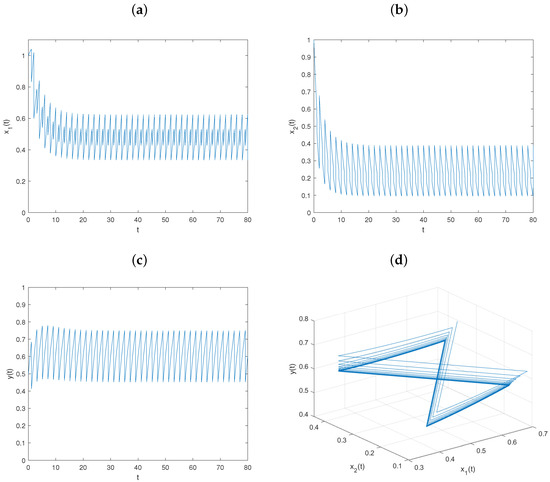
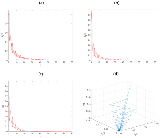
For biological considerations, all the parameters are assumed to be positive. And referring to references [26,27], the model parameters are set to $a_1=0.7,b_1=0.65,d_1=0.3,{\beta }_1=0.3,a_2=0.4,b_2=0.35,k_1=0.4,m_1=0.2,m_2=0.2,m_3=0.4,a_3=0.8,h_1=0.1,b_3=0.5,d_2=0.3,h_2=0.1,{\beta }_2=0.6,a_4=0.6,h_3=0.1,b_4=0.4,k_2=0.5,d=0.55,l=0.56,\sigma =2$. Then, $(1-d)(A+D)=1.6408>0.8696=1+(1-2d)AD$, ${\displaystyle (1-2d)AD=-0.1304<1}$, $ln\frac{1}{1-m_3}=0.5108<0.9966=a_2\xi \sigma +(a_4-h_3)(1-\xi )\sigma +\frac{k_1{\beta }_1(1-e^{-d_1\xi \sigma })}{d_1}{x_2}^{*}+\frac{k_2{\beta }_2(1-e^{-(d_2+h_2)(1-\xi )\sigma })}{(d_2+h_2)}{x_2}^{**}$, the conditions of Theorem 4, are satisfied with initial value $x_1(0)=1,x_2(0)=1,y(0)=0.5$, and system $(6)$ is permanent (see Figure 1). That is, the prey and predator populations will coexist.

Figure 1. Dynamical behavior of the permanence of system $(6)$: (a–c) time series of populations x, y, and z; (d) phase portrait of system (6).

5.1. The Effect of the Transient Impulsive Harvesting on Populations

Example 2. 

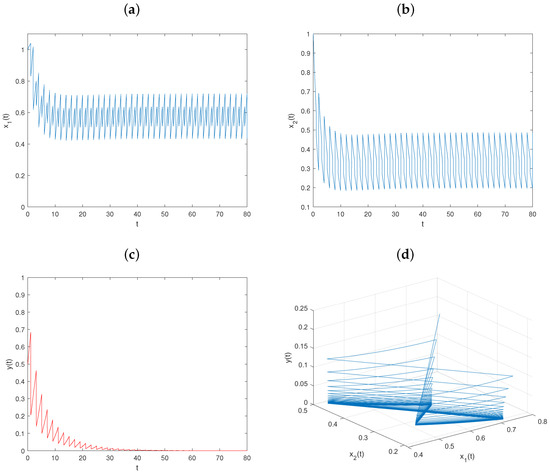
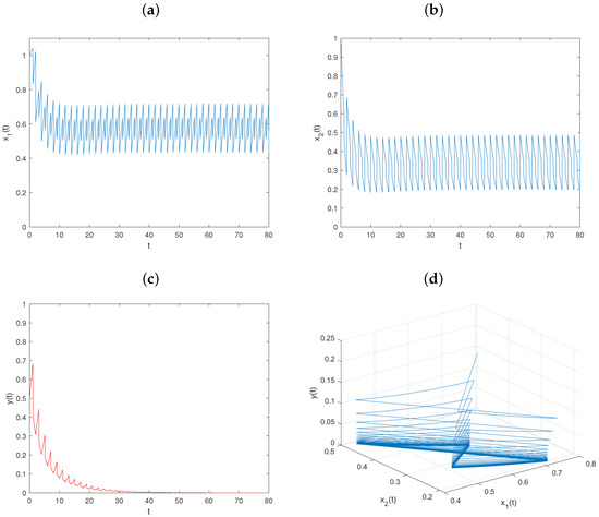
Let $m_3=0.7$ and keep fixed the values of other parameters, as in Figure 1. Then, $(1-d)(A+D)=1.6408>0.8696=1+(1-2d)AD$, ${\displaystyle (1-2d)AD=-0.1304<1}$, $(1-d)(AE+D)=0.5682<1$, $ln\frac{1}{1-m_3}=1.2040>0.9966=a_2\xi \sigma +(a_4-h_3)(1-\xi )\sigma +\frac{k_1{\beta }_1(1-e^{-d_1\xi \sigma })}{d_1}{x_2}^{*}+\frac{k_2{\beta }_2(1-e^{-(d_2+h_2)(1-\xi )\sigma })}{(d_2+h_2)}{x_2}^{**}$, and conditions (36)–(39) hold. From Theorem 2, the predator-extinction periodic solution $(\widetilde{x_1(t)},\widetilde{x_2(t)},0)$ of system $(6)$ is globally asymptotically stable (see Figure 2).

Figure 2. Dynamical behavior of system $(6)$ on predator-extinction periodic solution with $m_3=0.7$: (a–c) time series of populations x, y, and z; (d) phase portrait of system (6).

Example 3. 

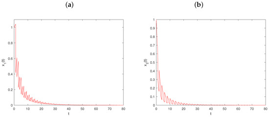
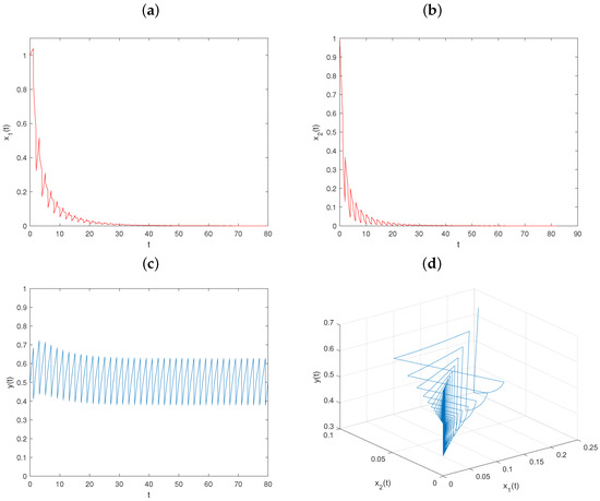
Let $m_1=0.6,m_2=0.5$, and keep fixed the values of other parameters, as in Figure 1. Then, $A_z=1.4582>1$, $(1-d)(A+D{E}_z)=0.7991<1$, $ln\frac{1}{1-m_3}=0.5108>-1.8039=a_2\xi \sigma +(a_4-h_3)(1-\xi )\sigma -\frac{a_2+b_2(e^{a_2\xi \sigma }-1)y^{*}}{a_2}-\frac{a_4-h_3+b_4(e^{(a_4-h_3)(1-\xi )\sigma }-1)y^{**}}{a_4-h_3}$, and conditions (64)–(66) hold. From Theorem 2, the prey-extinction periodic solution $(0,0,\widetilde{y(t)})$ of system $(6)$ is globally asymptotically stable (see Figure 3).

Figure 3. Dynamical behavior of system $(6)$ on prey-extinction periodic solution with $m_1=0.6,m_2=0.5$: (a–c) time series of populations x, y, and z; (d) phase portrait of system (6).

Example 4. 

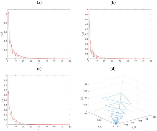
Let $m_1=0.6,m_2=0.5$, $m_3=0.7$, and keep fixed the values of other parameters, in as Figure 1. Then, $A_z=0.7291<1$, $(1-d)(A+D)=0.8430<1$, and conditions $(67)$ and $(68)$ hold. From Theorem 3, the trivial solution $(0,0,0)$ of system $(6)$ is globally asymptotically stable (see Figure 4).

Figure 4. Dynamical behavior of system $(6)$ on trivial solution with $m_1=0.6,m_2=0.5,m_3=0.7$: (a–c) time series of populations x, y, and z; (d) phase portrait of system (6).

Comparing Figure 1 and Figure 2, we can know that when $m_3=0.4$, the prey and predator populations coexist, while when $m_3=0.7$, the predator population goes extinct. Comparing Figure 1 and Figure 3, we can know that when $m_1=0.2,m_2=0.2$, the prey and predator populations coexist, while when $m_1=0.6,m_2=0.5$, the prey populations go extinct. From Figure 4, we can see that all the populations go extinct as $m_1=0.6,m_2=0.5,m_3=0.7$.

5.2. The Effect of Nontransient Impulsive Harvesting on Populations

Example 5. 

Let $h_3=0.9$, and keep fixed the values of other parameters, as in Figure 1. Then, $(1-d)(A+D)=1.6408>0.8696=1+(1-2d)AD$, ${\displaystyle (1-2d)AD=-0.1304<1}$, $(1-d)(AE+D)=0.5682<1$, $ln\frac{1}{1-m_3}=0.5108>0.2926=a_2\xi \sigma +(a_4-h_3)(1-\xi )\sigma +\frac{k_1{\beta }_1(1-e^{-d_1\xi \sigma })}{d_1}{x_2}^{*}+\frac{k_2{\beta }_2(1-e^{-(d_2+h_2)(1-\xi )\sigma })}{(d_2+h_2)}{x_2}^{**}$, and conditions $(36)$–$(39)$ hold. From Theorem 2, the predator-extinction periodic solution $(\widetilde{x_1(t)},\widetilde{x_2(t)},0)$ of system $(6)$ is globally asymptotically stable (see Figure 5).

Figure 5. Dynamical behavior of system $(6)$ on predator-extinction periodic solution with $h_3=0.9$: (a–c) time series of populations x, y, and z; (d) phase portrait of system (6).

Example 6. 

Let $h_1=0.9,h_2=0.9$, and keep fixed the values of other parameters, as in Figure 1. Then $A_z=1.4582>1$, $(1-d)(A+D{E}_z)=0.7768<1$, $ln\frac{1}{1-m_3}=0.5108>-1.8039=a_2\xi \sigma +(a_4-h_3)(1-\xi )\sigma -\frac{a_2+b_2(e^{a_2\xi \sigma }-1)y^{*}}{a_2}-\frac{a_4-h_3+b_4(e^{(a_4-h_3)(1-\xi )\sigma }-1)y^{**}}{a_4-h_3}$, and conditions $(64)$–$(66)$ hold. From Theorem 2, the prey-extinction periodic solution $(0,0,\widetilde{y(t)})$ of system $(6)$ is globally asymptotically stable (see Figure 6).

Figure 6. Dynamical behavior of system $(6)$ on prey-extinction periodic solution with $h_1=0.9,h_2=0.9$: (a–c) time series of populations x, y, and z; (d) phase portrait of system (6).

Example 7. 

Let $h_1=0.9,h_2=0.9$, $h_3=0.9$, and keep fixed the values of other parameters, as in Figure 1. Then, $A_z=0.7212<1$, $(1-d)(A+D)=0.8115<1$, and conditions $(67)$ and $(68)$ hold. From Theorem 3, the trivial solution $(0,0,0)$ of system $(2.1)$ is globally asymptotically stable (see Figure 7).

Figure 7. Dynamical behavior of system $(6)$ on trivial solution with $h_1=0.9,h_2=0.9$, $h_3=0.9$: (a–c) time series of populations x, y, and z; (d) phase portrait of system (6).

Comparing Figure 1 and Figure 4, we can know that when $h_3=0.1$, the prey and predator populations coexist, while when $h_3=0.9$, the predator population go extinct. Comparing Figure 1 and Figure 5, we can know that when $h_1=0.1,h_2=0.1$, the prey and predator populations coexist, while when $h_1=0.9,h_2=0.9$, the prey populations go extinct. From Figure 7, we can see that all the populations go extinct as $h_1=0.9,h_2=0.9$, $h_3=0.9$.

Figure 1, Figure 2, Figure 3, Figure 4, Figure 5, Figure 6 and Figure 7 show the global asymptotic stability of the boundary periodic solutions and the permanent extinction of system $(6)$ under the control of the transient/nontransient impulse harvesting rate, respectively. It is clear that with increasing transient/ nontransient impulsive harvesting rate, predator or prey populations cannot survive due to higher harvesting rate. The values of $m_3$, $h_3$, will not only directly affect the survival of the predator but also have an indirect effect on the prey. When $m_3$ or $h_3$ keeps increasing and exceeding the threshold, the predator population goes extinct and the population density of the prey populations increase accordingly. Similarly, The decrease in the density of predator population is observed as the prey populations go extinct, which is biologically reasonable.

6. Conclusions

In this paper, we propose a new predator–prey model to study the effects of transient/nontransient harvesting and pulse diffusion between prey on the prey and predator’s survival. Here, the predators live in their territory, which is patch 2, but the prey can impulsively diffuse between two patches. We focus on analyzing the dynamics of the investigated system generated by transient and nontransient impulsive harvesting to understand how predator and prey populations change when the system has an effect of harvesting. The main results of the present study are provided below:

(1)

All solutions of system $(6)$ are uniformly ultimately bounded.

(2)

If (36)–(39) hold, the solution $(\widetilde{x_1(t)},\widetilde{x_2(t)},0)$ of system $(6)$ is globally asymptotically stable.

(3)

If (64)–(66) hold, the solution $(0,0,\widetilde{y(t)})$ of system $(6)$ is globally asymptotically stable.

(4)

If (67)–(68) hold, the trivial solution of system $(6)$ is globally asymptotically stable.

(5)

The permanent conditions of system $(6)$ have also been established, that is

$$\begin{array}{c}(1-d)(A+D)>[1+(1-2d)AD],(1-2d)AD<1,\hfill \end{array}$$

and

$$\begin{array}{c}{\displaystyle ln\frac{1}{1-m_3}<a_2\xi \sigma +(a_4-h_3)(1-\xi )\sigma +\frac{k_1{\beta }_1(1-e^{-d_1\xi \sigma })}{d_1}{x_2}^{*}}\hfill \\ {\displaystyle +\frac{k_2{\beta }_2(1-e^{-(d_2+h_2)(1-\xi )\sigma })}{(d_2+h_2)}{x_2}^{**}.}\hfill \end{array}$$

In addition, from numerical simulations and theorems, we can deduce that there exist a predator transient impulsive harvesting threshold ${m_3}^{*}$ and a nontransient impulsive harvesting threshold ${h_3}^{*}$. When $m_3>{m_3}^{*}$ or $h_3>{h_3}^{*}$, the predator population z goes extinct. When $m_3<{m_3}^{*}$ or $h_3<{h_3}^{*}$, system $(6)$ is permanent. In addition, there must exist thresholds ${m_1}^{*},{m_2}^{*}$ and ${h_1}^{*},{h_2}^{*}$. When $m_1>{m_1}^{*}$ and $m_2>{m_2}^{*}$, or $h_1>{h_1}^{*}$ and $h_2>{h_2}^{*}$, the prey populations x and y go extinct. When $m_1<{m_1}^{*}$ and $m_2<{m_2}^{*}$, or $h_1<{h_1}^{*}$ and $h_2<{h_2}^{*}$, system $(6)$ is permanent. Therefore, we must choose a suitable harvesting rate smaller than the value of the harvesting threshold when hunting both prey and predator for economic interest. Reducing the amount of transient or nontransient impulsive harvesting is significant for preventing population extinction so as to maintain ecological balance.

In future work, we can continue to study the optimal harvest strategy of system $(6)$ to explore the maximum sustainable yield and the corresponding harvest effort of system $(6)$ [28,29]. We can also consider impulsive delayed harvesting or stage structure of prey/predator populations, which will lead to richer dynamics [30]. In addition, trying to solve system $(6)$ using an intelligent computational solver, or different numerical methods such as the Galerkin method or Legendre wavelet algorithm will also be interesting work [31,32,33].

References

- Brauer, F.; Soudack, A. Stability regions in predator–prey systems with constant-rate prey harvesting. J. Math. Biol. 1979, 8, 55–71. [Google Scholar] [CrossRef]
- Kumar, S.; Kharbanda, H. Chaotic behavior of predator–prey model with group defense and non-linear harvesting in prey. Chaos Solitons Fractals 2018, 119, 19–28. [Google Scholar] [CrossRef]
- Lv, Y.; Yuan, R.; Pei, Y. A prey-predator model with harvesting for fishery resource with reserve area. Appl. Math. Model. 2013, 37, 3048–3062. [Google Scholar] [CrossRef]
- Liu, X.; Chen, L. Global dynamics of the periodic logistic system with periodic impulsive perturbations. J. Math. Anal. Appl. 2004, 289, 279–291. [Google Scholar] [CrossRef]
- Tian, Y.; Gao, Y.; Sun, K. Global dynamics analysis of instantaneous harvest fishery model guided by weighted escapement strategy. Chaos Solitons Fractals 2022, 164, 112597. [Google Scholar] [CrossRef]
- Liu, J.; Hu, J.; Yuen, P. Extinction and permanence of the predator–prey system with general functional response and impulsive control. Appl. Math. Model. 2020, 88, 55–67. [Google Scholar] [CrossRef]
- Wei, C.; Liu, J.; Chen, L. Homoclinic bifurcation of a ratio-dependent predator–prey system with impulsive harvesting. Nonlinear Dyn. 2017, 89, 2001–2012. [Google Scholar] [CrossRef]
- Jiao, J.; Liu, Z.; Li, L.; Nie, X. Threshold dynamics of a stage-structured single population model with non-transient and transient impulsive effects. Appl. Math. Lett. 2019, 97, 88–92. [Google Scholar] [CrossRef]
- Tao, X.; Zhu, L. Study of periodic diffusion and time delay induced spatiotemporal patterns in a predator–prey system. Chaos Solitons Fractals 2021, 150, 13–14. [Google Scholar] [CrossRef]
- Wang, L.; Liu, Z.; Chen, L. Impulsive diffusion in single species model. Chaos Solitons Fractals 2006, 33, 1213–1219. [Google Scholar] [CrossRef]
- Mishra, P.; Raw, S.; Tiwari, B. On a cannibalistic predator–prey model with prey defense and diffusion. Appl. Math. Model. 2021, 90, 165–190. [Google Scholar] [CrossRef]
- Sugden, A.; Pennisi, E. When to Go, Where to Stop. Science 2006, 313, 775. [Google Scholar] [CrossRef]
- Takeuchi, Y. Global Dynamical Properties of Lotka-Volterra System; World Scientific: Singapore, 1996. [Google Scholar]
- Hui, J.; Chen, L. A single species model with impulsive diffusion. Acta Math. Appl. Sin. 2005, 21, 43–48. [Google Scholar] [CrossRef]
- Cui, J. The effect of diffusion on the time varying logistic population growth. Comput. Math. Appl. 1998, 36, 1–9. [Google Scholar] [CrossRef][Green Version]
- Zhong, Z.; Zhang, X.; Chen, L. The effect of pulsed harvesting policy on the inshore-offshore fishery model with the impulsive diffusion. Nonlinear Dyn. 2011, 63, 537–545. [Google Scholar]
- Jiao, J.; Cai, S.; Chen, L. Dynamical Analysis of a three-dimensional predator–prey model with impulsive harvesting and diffusion. Int. J. Bifurcat. Chaos 2011, 21, 453–465. [Google Scholar] [CrossRef]
- Dhar, J.; Jatav, K.S. Mathematical analysis of a delayed stage-structured predator–prey model with impulsive diffusion between two predators territories. Ecol. Complex. 2013, 16, 59–67. [Google Scholar] [CrossRef]
- DuTemple, L.A.; Stone, L.M. Tigers; Lerner Publications: Minneapolis, MN, USA, 1996. [Google Scholar]
- Seidensticker, J. Tigers; MBI Publishing Company: Saint Paul, Brazil, 1996. [Google Scholar]
- Bainov, D.; Simeonov, P. Impulsive Differential Equations: Periodic Solutions and Applications; Longman Scientific and Technical, 1993. [Google Scholar]
- Jury, E. Inners and Stability of Dynamic Systems; Wiley: New York, NY, USA, 1974. [Google Scholar]
- Smith, H. Cooperative systems of differential equations with concave nonlinearities. Nonlinear Anal. TMA 1986, 10, 1037–1052. [Google Scholar] [CrossRef]
- Jiao, J.; Tang, W. Dynamics of a lake-eutrophication model with nontransient/transient impulsive dredging and pulse inputting. Adv. Differ. Equ. 2021, 2021, 1–16. [Google Scholar] [CrossRef]
- Lakshmikantham, V. Theory of Impulsive Differential Equations; World Scientific: Singapore, 1989. [Google Scholar]
- Wang, J.; Cheng, H.; Liu, H.; Wang, Y. Periodic solution and control optimization of a prey-predator model with two types of harvesting. Adv. Differ. Equ. 2018, 2018, 41. [Google Scholar] [CrossRef]
- Li, Y.; Cui, J.; Song, X. Dynamics of a predator–prey system with pulses. Appl. Math. Comput. 2008, 204, 269–280. [Google Scholar] [CrossRef]
- Lawson, J.; Braverman, E. Optimality and sustainability of delayed impulsive harvesting. Commun. Nonlinear Sci. 2022, 117. [Google Scholar] [CrossRef]
- Zhang, X.; Shuai, Z.; Wang, K. Optimal impulsive harvesting policy for single population. Nonlinear Anal. Real World Appl. 2003, 4, 639–651. [Google Scholar] [CrossRef]
- Amit, S.; Gupta, B.; Dhar, J.; Srivastava, S.K.; Sharma, P. Stability analysis and optimal impulsive harvesting for a delayed stage-structured self dependent two compartment commercial fishery model. Int. J. Control 2021, 10, 1119–1129. [Google Scholar]
- Umar, M.; Sabir, Z.; Raja, M.A.Z.; Amin, F.; Saeed, T.; Sanchez, Y.G. Design of intelligent computing solver with Morlet wavelet neural networks for nonlinear predator–prey model. Appl. Soft Comput. 2023, 134, 109975. [Google Scholar] [CrossRef]
- Ruttanaprommarin, N.; Sabir, Z.; Said, S.B.; Raja, M.A.Z.; Bhatti, S.; Weera, W.; Botmart, T. Supervised neural learning for the predator–prey delay differential system of Holling form-III. AIMS Math. 2022, 7, 20126–20142. [Google Scholar] [CrossRef]
- Jitendra; Chaurasiya, V.; Rai, K.N.; Singh, J. Legendre wavelet residual approach for moving boundary problem with variable thermal physical properties. Int. J. Nonlinear Sci. Numer. Simul. 2022, 23, 957–970. [Google Scholar] [CrossRef]
Disclaimer/Publisher’s Note: The statements, opinions and data contained in all publications are solely those of the individual author(s) and contributor(s) and not of MDPI and/or the editor(s). MDPI and/or the editor(s) disclaim responsibility for any injury to people or property resulting from any ideas, methods, instructions or products referred to in the content. |
© 2023 by the authors. Licensee MDPI, Basel, Switzerland. This article is an open access article distributed under the terms and conditions of the Creative Commons Attribution (CC BY) license (https://creativecommons.org/licenses/by/4.0/).