Article

Modeling the Dynamics of Negative Mutations for a Mouse Population and the Inverse Problem of Determining Phenotypic Differences in the First Generation

1
Department of Mathematics, Faculty of Physics, Lomonosov Moscow State University, Moscow 119991, Russia
2
Department of Byophysics, Faculty of Physics, Lomonosov Moscow State University, Moscow 119991, Russia
3
Sobolev Insitute of Mathematics, Novosibirsk 630090, Russia
4
Institute of Computational Mathematics and Mathematical Geophysics SB RAS, Novosibirsk 630090, Russia
*
Author to whom correspondence should be addressed.
Mathematics 2023, 11(14), 3180; https://doi.org/10.3390/math11143180
Submission received: 26 June 2023 / Revised: 17 July 2023 / Accepted: 18 July 2023 / Published: 20 July 2023

Abstract

:
This paper considers a model for the accumulation of mutations in a population of mice with a weakened function of polymerases responsible for correcting DNA copying errors during cell division. The model uses the results of the experiment published by Japanese scientists, which contain data on the accumulation of phenotypic differences in three isolated groups of laboratory mice. We have developed a model for the accumulation of negative mutations. Since the accumulation of phenotypic differences in each of the three groups of mice occurred in its own way, we assumed that these differences were associated with genotypic differences in the zeroth generation and set the inverse problem of determining the initial distribution of these differences. Additional information for solving the inverse problem was a set of experimental data on the number of mutant lines and the number of individuals in each group of mice. The results obtained confirmed our assumption.

1. Introduction

Mutations are a necessary condition for evolution and the main source of genetic information in the process of speciation. The effects of mutations, depending on internal and external factors, can be beneficial, harmful, or neutral, and the pace of evolution depends on the rate of mutations.
The occurrence of mutations as errors in DNA replication (copying) is associated with the presence of constant fluctuations, both “internal” and “external”. The latter include the parameters of the environment: temperature, pH, elemental composition of the environment, ultraviolet and ionizing radiation, etc. In addition, the presence of a complex enzymatic array of proteins affects the process of DNA replication. Recombination (the redistribution of DNA parts) is the process during which chromosomes exchange genetic material. This process contributes to the acceleration of new feature fixes. In this case, new combinations (meiosis) of the genetic material of the parents are created, which are transmitted to posterity [1].
To maintain the integrity of the species, the continuity of generations is necessary, for which the genetic information contained in the cell must be accurately transferred to the daughter cells. DNA replication with very high precision is provided by the action of DNA polymerases. Typically, replication occurs with high fidelity due to the combined action of DNA polymerases and the mismatch repair system (MMR) [2]. The accuracy of DNA replication depends on the nucleotide selectivity of DNA polymerase, its correcting activity, and the ability to repair mismatched nucleotides. Polymerases make mistakes approximately once for every 10 4 10 5 polymerized nucleotides [2,3]. Corrective activity increases the overall accuracy of DNA synthesis by 10 2 10 3 times, depending on the specific DNA polymerase and the nature of the error. The mismatch repair system recognizes and corrects insertions, omissions, and wrongly paired bases that are the direct product of DNA polymerase errors during DNA replication. MMR increases the accuracy of DNA replication by up to three orders of magnitude [4,5,6,7]. The bulk of DNA synthesis in the eukaryotic cell occurs during the replication of intact DNA templates. These syntheses are catalyzed by the α , δ , and ε families of polymerases for nuclear DNA and by the family of γ polymerases for mitochondrial DNA. These four DNA polymerases are highly accurate, generating on average less than one base substitution or one base insertion/deletion for every 100,000 correct events [8].
DNA polymerase δ is the main enzyme for DNA replication and genome maintenance. It contributes to the correct synthesis of DNA due to its internal 3′-5′ exonuclease corrective activity [9,10] responsible for removing misplaced nucleotides that are unable to form a correct pair with the corresponding template nucleotide before further chain extension. In addition, studies [11,12] have shown that polymerase δ plays an important role in the replication of both leading and lagging DNA strands. The catalytic and corrective subunit of the DNA polymerase δ complex, POLD1, plays a crucial role in the processes of DNA replication and repair [13]. Mutations in POLD1 are associated with abnormal cell division in various human tumors [14]. However, the significance of altered POLD1 expression in cancer and its usefulness as a prognostic factor are not fully understood [15].
Fitness, as the ability to reproduce among individuals with a certain range of characteristics that allow them to survive in specific conditions and continue the genus, is determined by a favorable combination of mutation and reparation processes. Many mutation models describe the dynamics of fitness as a wave process with a constant speed, where deterministic patterns are applied to describe selection and random patterns are responsible for genetic drift [16,17]. In some wave models of mutations [18,19], the concepts of “mutator” (a mutant copy of a gene that provides an increase in the mutation rate) and “antimutator” (a mutant copy of a gene that provides a decrease in the mutation rate) are used [20], and it is believed that selection contributes to maintaining the optimal frequency of occurrence of alleles (different variants of the same gene) of “mutator” and “antimutator” in a population [19].
In [21], a model for the accumulation of negative mutations in a population of mice is presented based on experimental data published in [22] on the estimation of the mutation rate of four groups of mice: three groups of laboratory-type mice and one group of wild-type mice. The groups differed in the original pair of mice that gave rise to each group. Unlike wild-type mice, the corrective activity of δ polymerase, an enzyme that promotes precise DNA synthesis, was disabled in laboratory mice [9,10,11]. In this sense, all laboratory mice were considered mutants. In each of the three groups of laboratory mice, ones with visible (phenotypic) differences appeared due to the accumulation of mutations, giving rise to a new mutant line. (A mutant line is a group of individuals that originated from one pair of mice and do not have visible differences). Figure 1 schematically shows the process by which new mutant lines emerge in each group of mice from generation to generation. Each isolated group of mice is marked with a separate color. Each circle represents a group of phenotypically identical individuals. Circles at the same horizontal level correspond to the same generation in the mouse population. The lines connecting the circles represent the transition from the generation of parents to the generation of children. Each mutant line in the scheme is traced as a set of circles connected by vertical lines. If a certain group of parents gave birth to mice with phenotypic differences, then several straight lines would depart from the corresponding circle. Each line branching off to the side means a transition from parents to descendants phenotypically different from the latter. Thus, we denote the emergence of a new mutant line, individuals of which can reproduce their own kind. The number of phenotypically distinct groups in each generation can be determined by the number of circles that are at the same horizontal level.
According to the results in [22], disabling the corrective activity of δ polymerase in experiments with mice led to a 17-fold increase in the rate of the negative mutations’ accumulation for three groups of laboratory-type mice relative to the wild-type group and further to a significant decrease in the number of different mutant lines from the 12th to the 20th generation. The consequences of the accumulated harmful mutations included a decrease in body weight, mortality of individuals (about 30% of mutant mice died from thymus lymphoma at the age of 3–8 months), fertility decline, infertility, etc. The average body weight of all mutant mice decreased as the number of generations increased; weight loss per generation was 0.115 g in males and 0.090 g in females, especially in mutant lines with numerous generations. The most striking phenotypic difference between the mutant and wild-type mice was noted in reproductive ability. If the ability of wild-type mice to reproduce remained almost constant, then the same ability of the mutants decreased significantly and non-linearly, most intensively in the first generations. As the number of generations increased, the average number of offspring per mating decreased by 0.042 per generation. The authors of the experiment did not exclude the possibility of various phenotypic differences in the mutant lines as a result of genetic variations in the original individuals; however, it is more likely that most of the phenotypic changes were associated with a higher mutation rate in subsequent generations. At the same time, the accumulation of phenotypic differences in each of the three groups of laboratory mice occurred differently. It is natural to assume that these differences were associated with genotypic differences in the original pairs, since this factor significantly affects the dynamics of the negative mutations’ accumulation in the population and their threshold level, from which the number of individuals decreases sharply.
The original model presented in [21] consisted of two first-order ordinary differential equations. The question of phenotypic differences in the first generation of mice remained open during the study.
According to the model in the present paper, the process of mutation propagation in a population is described by the diffusion equation. In this approach, the size of the population acts as the spatial coordinate x. Time t is measured in generations.
We assume that the number of phenotypic differences in the first generation depends on the initial number of mutants in the population. In this work, the value to be determined is the distribution of the number of phenotypic differences in the first generation, depending on the size of the initial population. The analysis is based on known data on the dynamics of the mutant line’s formation over generations.
The rest of the article is organized as follows. In the section “Materials and Methods”, we discuss the biophysical model and provide a direct problem statement for determining the number of accumulated negative mutations. Also in this section, we present the formulation and algorithm for solving the inverse problem, the purpose of which is to determine the number of phenotypic differences in the first generation. In the “Results” section, we present the results of a numerical solution of the inverse problem for two test examples as well as for a model problem in which experimental data are used as additional information. In the “Discussion” section, we discuss the mathematical aspects of the reverse problem with the a priori data set on the curve and also explain the biophysical meaning of the result. In the “Conclusions section”, we briefly formulate the results of our work.

2. Materials and Methods

The model describing the process of mutation accumulation consists of two equations:
u t D u 2 u x 2 = A T * u v ( x , t t 0 ) q ( x ) u γ ( x ) + ( 1 β ) v ( x , t t 0 ) , v t = B T * γ ( x ) v .
The first equation is a non-linear diffusion equation for the function u ( x , t ) , whose value at each point of the phase space ( x , t ) means the number of accumulated phenotypic differences in generation t in the current population x. It should be noted that in the experiment described in [22], three groups of laboratory mice initially became mutants by disabling δ polymerase activity. Each of the three groups of mice developed independently of the others, so we consider each of these groups to be a separate population. It follows from the obtained experimental data that the number of laboratory mutant mice with the disabled δ polymerase activity function did not exceed 20 individuals; therefore, the interval [ 0 , 20 ] is chosen in the model as the x-variable interval. The experimental data published in [22] contain information about mutant lines of laboratory mice up to the 20th generation, so in this paper we consider the time interval t [ 0 , 20 ] .
The process inhibitor, v ( x , t ) , is the δ polymerase corrective activity function, which characterizes the number of phenotypic differences blocked as a result of its activity. Based on data from the above literature, it can be concluded that the corrective activity of δ polymerase makes the greatest contribution to the accuracy of DNA copying and error correction compared to other corrective factors, such as MMR. That explains the choice of the inhibitor of the negative mutations’ accumulation in the model. Furthermore, this allowed us to choose the model parameters based on the available experimental data on the effect of disabling the corrective activity of δ polymerase on the accumulation of mutations in the mouse population.
The parameters in (1) are the time delay t 0 , the number of generations during which there was a slow accumulation of mutations and the number of phenotypic differences did not change, and the diffusion coefficient of the activator D u , which we assume is equal to the average change in the number of phenotypic differences from generation to generation. Using the experimental data from [22], we accept D u = 1 ; T * = 1 (generation) is a constant introduced to match the dimensions; and constant A is the rate of the activator change, which is the probability of δ polymerase error in the absence of corrective activity, but taking into account the influence of the mismatched nucleotide repair complex. We accept A = 10 8 mutations per nucleotide [8]; constant B is the rate of the inhibitor change, which is the probability of δ polymerase error in the presence of corrective activity and the mismatch repair complex. The accuracy of DNA synthesis is ensured by the selectivity of the polymerase itself (the error probability is 10 5 ) [8], the exonuclease activity of the polymerase, which reduces the error probability by 100 times, and the mismatched nucleotide repair complex, which reduces the error probability by 100 times. Thus, the resulting DNA synthesis error probability is 10 10 [8]. We accept B = 10 10 mutations per nucleotide. By multiplying A and B by the size of the mouse genome equal to 2,717,000,000 bp (base pairs) [23], we obtain the following values of the activator and inhibitor change rates for our model: A = 27.17 , B = 0.2717 , which we will further use in numerical experiments. The constant β is the kinetic coefficient of interaction between the activator and the inhibitor and is determined by the ratio of the error probability of δ polymerase with normal corrective activity to the error probability of δ polymerase with disabled corrective activity, β = B / A = 0.01 [8]. The function γ ( x ) sets the threshold value for the number of accumulated negative mutations for a group of mutant mice with disabled δ polymerase corrective activity, which leads to the elimination of its carriers. We consider the threshold for each group of mice to be the maximum number of phenotypic differences accumulated in this group over the entire observation period. Based on the analysis of graphs built on the basis of experimental data, it is assumed in the model that normalized values of γ ( x ) can be set as γ ( x ) = k e b x k , where k = 1.84835308 , b = 0.18203879 . The function q ( x ) specifies the number of genome mutations in the zeroth generation. In its meaning, it is the initial condition for the activator: u ( x , 0 ) = q ( x ) . Thus, the inequality q ( x ) γ ( x ) , x [ 0 , 20 ] is to be held. We have taken into account that the inhibitory effect of polymerases starts at the initial time t = 0 , so we consider v ( x , 0 ) = 0 at 0 x 20 . In view of the fact that the function v enters the first equation with a time-delayed argument, we extend it by continuity: v = 0 , for t < t 0 .
We set the boundary conditions for the first equation as follows: u ( 0 , t ) = 0 , which means that if there are no mutants in the population, the number of new mutations is zero, and u ( 20 , t ) = 0 , since the number of mutant lines decreased sharply at x > 15 .
The choice of this model for describing the negative mutations’ accumulation is related to the following properties of the solution of the system under consideration, which were analyzed in [24,25]. The solution of the second equation can be obtained explicitly:
v ( x , t ) = γ ( x ) 1 e B t / T * , t 0 , 0 x L , v ( x , t ) = 0 , t < 0 , 0 x L .
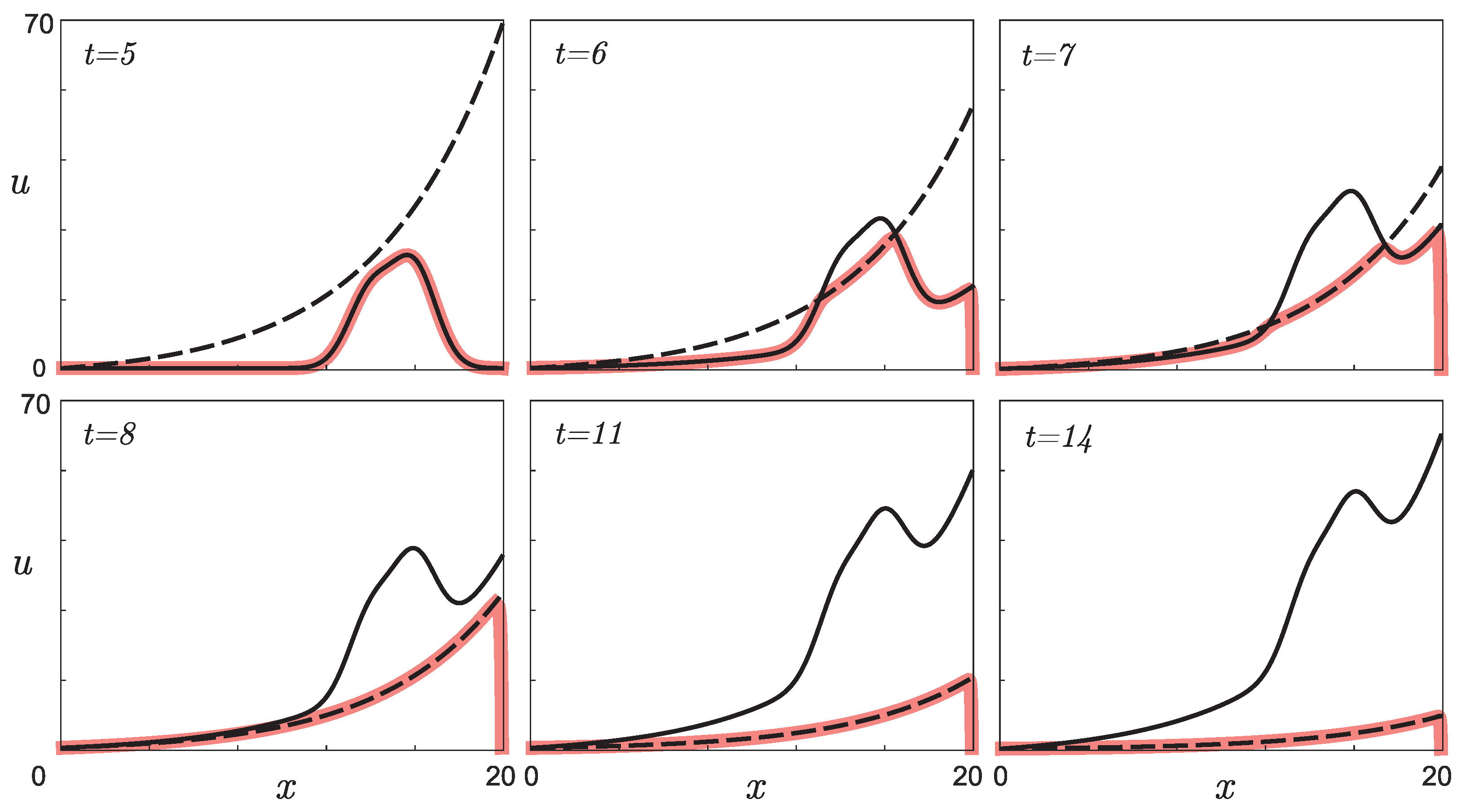
Here we denoted the x-variable interval as [ 0 , L ] . Thus, the dependence v ( x , t ) in the first equation can be considered known. The right side of the first equation is a quadratic polynomial whose roots are the functions u 1 ( x , t ) = v ( x , t t 0 ) + q ( x ) and u 2 ( x , t ) = γ ( x ) ( 1 β ) v ( x , t t 0 ) . According to the results of [24,25], the solution of the differential equation attracts the smallest of these functions. Figure 2 illustrates the direct problem solution as a function of time. Due to the inequality q ( x ) γ ( x ) , x [ 0 , 20 ] , and the choice of the initial condition u ( x , 0 ) = q ( x ) , taking into account the fact that v ( x , t t 0 ) = 0 for t < t 0 , the value of the function u 1 ( x , t ) = q ( x ) corresponds to the stable equilibrium of the first equation of system (1), so it does not change with time until t t 0 . For t > t 0 and small values of v ( x , t t 0 ) such that for every x [ 0 , 20 ] the inequality u 1 ( x , t ) < u 2 ( x , t ) holds, the function u ( x , t ) attracts the values of the function u 1 ( x , t ) (solid black line in Figure 2). As t grows, the inequality u 2 ( x , t ) < u 1 ( x , t ) becomes valid, and the solution attracts the function u 2 ( x , t ) (dashed black line in Figure 2). Since for sufficiently large t, the function v ( x , t ) takes values close to γ ( x ) , then the values of u 2 ( x , t ) become close to zero over time, and the function u ( x , t ) tends to this value.
This behavior of the direct problem solution can be interpreted as follows: an increase in the number of negative mutations over time causes an increase in the inhibitor. At some point in time, for a population consisting of x individuals, equality q ( x ) + 2 v ( x , t ) = γ ( x ) will be satisfied. This moment can be considered the moment when the inhibitor reaches its threshold value, which corresponds to the maximum possible level of accumulated negative mutations. Such numerous negative mutations cause the extinction of the population and a decrease in the number of individuals, which naturally leads to a decrease in the total number of phenotypic differences in the remaining mice.
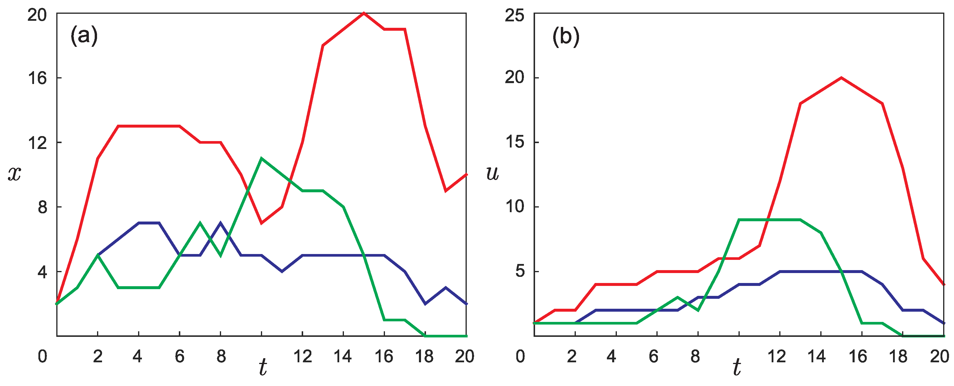
In [21], on the basis of a scheme similar to Figure 1 but containing real experimental data, the graphs presented in Figure 3b were made. The number of mutant lines in each generation was calculated by counting the circles located in the scheme at the same horizontal level. The method of obtaining the point values for the curves in Figure 3a is described in the Appendix. The graphs in Figure 3 served as a prioriinformation that was used in the course of solving the inverse problem.
Figure 3a shows three curves in the phase space ( x , t ) , each of which corresponds to one of the three groups of laboratory mice described in the experiment [22]. Each node on the curve represents the number of individuals in a given generation for the corresponding mutant group.
Each point of the graph shown in Figure 3b can be considered the value of u ( x , t ) corresponding to the relative node in Figure 3a.
Each of the three original pairs of laboratory mutant mice with disabled polymerase activity had certain genotypic differences due to which in each of the three groups the accumulation of mutations occurred differently, which led to the formation of new mutant lines in each group. Phenotypic differences came out in subsequent generations as a result of the genotypic differences’ accumulation.
Since there was no experimental information on phenotypic differences for each of the three pairs of mice in the zero generation, when constructing the experimental curves, we considered that all three pairs correspond to the same value, x = 2 .
We formulate the direct problem based on the model as follows:
u t 2 u x 2 = λ 1 u v ( x , t t 0 ) q ( x ) u γ ( x ) + λ 2 v ( x , t t 0 ) , x ( 0 , L ) , t ( 0 , T ] , u ( 0 , t ) = 0 , u ( L , t ) = 0 , t ( 0 , T ] , u ( x , 0 ) = q ( x ) , x [ 0 , L ] .
Here, λ 1 : = A / T * , λ 2 = 1 β , t 0 are given parameters, the function q ( x ) is smooth, and the function γ ( x ) is continuous for all x [ 0 , L ] .
The function v ( x , t ) is equal to zero for t < 0 , and for t 0 it is defined as a solution to the Cauchy problem:
v ( x , t ) t = B T * v ( x , t ) + γ ( x ) , t ( 0 , T ] , v ( x , 0 ) = 0 ,
where x [ 0 , L ] acts as a parameter. This function has an explicit form (2).
The direct problem is to obtain the function u ( x , t ) in the domain D ( x , t ) ( 0 , 1 ) × ( 0 , T ] from known values of parameters λ 1 , 2 , t 0 , given distributions q ( x ) and γ ( x ) and a known expression (2) for v ( x , t ) . The existence of a solution to the direct problem, whose behavior is illustrated in Figure 2, was proved in [25].
The solution of the inverse problem is focused on obtaining the number of mutants in the first generation for the groups of mice described in the experimental work of [22] for which the corrective activity of δ polymerase was disabled.
The inverse problem is to retrieve the function q ( x ) , x [ 0 , L ] from the known additional information about the values of the function u ( x , t ) on the known curves
x i ( t ) = f 1 i ( t ) , u x i ( t ) , t = f 2 i ( t ) , t [ 0 , T ] , i = 1 , I ¯ ,
where I is the number of known curves.
The solution to the inverse problem (3) and (4) can be found as a function q ( t ) realizing the minimum of the functional
J [ q ] = i = 1 I 0 T u f 1 i ( t ) , t ; q f 2 i ( t ) 2 d t + α Ω [ q ] .
Here, Ω [ q ] is a smoothing functional. In this paper, we use Ω [ q ] q W 2 1 2 :
Ω [ q ] = 0 L q 2 ( x ) + q 2 ( x ) d x .
Also in (5), u ( x , t ; q ) is a solution to the direct problem (3) for the given function q ( t ) , and α is the regularization parameter, which can be chosen, for example, in accordance with the generalized residual principle [26].
The function q ( x ) realizing the minimum of the functional (5) can be found using gradient minimization methods, for example, the steepest descent method [27].
Algorithm for solving the inverse problem:
1.
Setting s : = 0 and q ( 0 ) ( x ) as the initial approximate value.
2.
Obtaining the solution u ( s ) ( x , t ) to the direct problem:
u ( s ) t 2 u ( s ) x 2 = λ 1 u ( s ) v ( x , t t 0 ) q ( s ) ( x ) ( u ( s ) γ ( x ) + + λ 2 v ( x , t t 0 ) ) , x ( 0 , L ) , t ( 0 , T ] , u ( s ) ( 0 , t ) = 0 , u ( s ) ( L , t ) = 0 , t ( 0 , T ] , u ( s ) ( x , 0 ) = q ( s ) ( x ) , x [ 0 , L ] .
3.
Obtaining the solution ψ ( s ) ( x , t ) to the adjoint problem:
ψ ( s ) t + 2 ψ ( s ) x 2 + λ 1 ψ ( s ) 2 u ( s ) γ ( x ) + ( λ 2 1 ) v ( x , t t 0 ) q ( s ) ( x ) = = 2 i = 1 I δ x f 1 i ( t ) u x , t ; q ( s ) f 2 i ( t ) , x ( 0 , L ) , t [ 0 , T ) , ψ ( s ) ( 0 , t ) = 0 , ψ ( s ) ( L , t ) = 0 , t [ 0 , T ) , ψ ( s ) ( x , T ) = 0 , x [ 0 , L ] .
Here, δ ( x ) is the Dirac delta function.
4.
Obtaining the gradient of the functional (5):
J q ( s ) ( x ) = λ 1 0 T ψ ( s ) ( x , t ) u ( s ) γ ( x ) + λ 2 v ( x , t t 0 ) d t ψ ( s ) ( x , 0 ) + α Ω [ q ( s ) ] ( x ) .
5.
Expressing an approximate solution at the next iteration step:
q ( s + 1 ) ( x ) = q ( s ) ( x ) β s J q ( s ) ( x ) ,
where β s is a descent parameter.
6.
Checking the condition for stopping the iterative process. If it holds, then we set q inv ( x ) : = q ( s + 1 ) ( x ) as the solution to the inverse problem. Otherwise, we set s : = s + 1 and go to step 2.
(a)
In the case of data measured in an experiment with errors, δ i , i = 1 , I ¯ , the stopping criterion is
i = 1 I 0 T u f 1 ( t ) , t ; q ( s + 1 ) ( t ) f 2 i δ i ( t ) 2 d t i = 1 I δ i 2 .
Here, δ i are error estimates for the input data f 2 i , i = 1 , I ¯ , observed experimentally:
f 2 i f 2 i δ i L 2 δ i , i = 1 , I ¯ .
(b)
In the case of exact input data, the iterative process stops when J q ( s ) is less than the error estimate of the finite difference approximation.
The use of a priori information on the solution can significantly reduce the number of iterations of the gradient method [28]. When projecting an approximate solution into the required function class, one can obtain an estimate for the strong convergence of gradient methods [28] by means of the theory of Fejer operators [29]. In dynamic inverse problems, the adjoint problem and the gradient of the functional can be calculated simultaneously at each moment of time, which reduces the required memory and speeds up the calculations [30].

3. Results

In this section, model examples of solving the inverse problem (3) and (4) will be given. We will demonstrate both an example in which the curves for setting the input data (4) well cover the entire area of the function q ( x ) definition and an example in which the curves cover only a part of this area.

3.1. A Model Example with a Set of Curves That Well Cover the Region of the Unknown Function q ( x ) Definition

Here we consider the operation of the proposed algorithm based on the minimization of objective functional (5) on a model example of the inverse problem (3) and (4) solving given the following set of parameters:
λ 1 = 27.17 , λ 2 = 0.99 , t 0 = 5 , L = 20 , T = 20 , γ ( x ) = k e b x k , k = 1.84835308 , b = 0.18203879 , B T * = 0.27 , q ( x ) q model ( x ) = 15 exp 1 2 ( x 14 ) 2 + 20 exp 1 2 ( x 16 ) 2 .
We set the following model functions as input data:
f 1 1 ( t ) = 4 sin ( t ) + 4 , f 1 2 ( t ) = 4 sin ( t ) + 10 , f 1 3 ( t ) = 4 sin ( t ) + 16 .
For the specified set of parameters, using the solution of the direct problem (6), we simulated the functions f 2 i ( t ) , i = 1 , I ¯ , I = 3 according to the following algorithm.
  • Introducing the following uniform grids:
    T M = t m , 0 m M : t m = 0 + τ m , τ = T / M ,
    X N = x n , 0 n N : x m = 0 + h n , h = L / N .
  • Solving the direct problem (3) numerically on uniform meshes (11) and (12) for the known function q ( x ) q model ( x ) . Thus, we obtain a set of grid values u ( x n , t m ) , n = 0 , N ¯ , m = 0 , M ¯ .
  • Obtaining the values of the function u ( x , t m ) for x = f 1 i ( t m ) for each t m by using the inverse interpolation method:
    f 2 i ( t m ) = u f 1 i ( t m ) , t m , i = 1 , I ¯ .
    Thus, we obtain the grid values of the functions f 2 i ( t m ) , m = 0 , M ¯ , i = 1 , I ¯ .
Remark 1. 
To solve the direct and adjoint problems (7), we used the stiff method of lines SMOL [31], which makes it possible to reduce the partial differential equations’ system to a system of ordinary differential equations. The latter were solved using the one-stage Rosenbrock scheme with complex coefficients (CROS1) [32].
Remark 2. 
To calculate the derivative Ω [ q ( s ) ] ( x ) in (8), we used an approach based on pre-sampling the smoothing functional Ω [ q ] followed by analytical differentiation of the resulting formulas on a uniform mesh (12).
Remark 3. 
The parameters α and β s in numerical calculations were chosen heuristically based on numerical experiments in such a way that the value of the minimized functional was a monotonically decreasing function of the iteration number.
All numerical results were obtained using the original author’s codes.
When implementing the steepest descent method described in Section 2, we used uniform meshes (11) and (12) with N = 200 and M = 200 , the descent parameter β s = 3.5 × 10 3 , the regularization parameter α = 1 , the number of iterations of the gradient method S = 3000 , and the initial approximation q ( 0 ) ( x ) 0 . When solving the adjoint problem (7), the following expression was used to approximate the delta function [33]:
δ ^ ( x ) = 1 ω 1 | x ω | , | x ω | 1 , 0 , | x ω | > 1 ,
where ω is the size of the delta function’s discrete support. In this example, we set ω = 0.01 . To calculate the integral in (8), we used the trapezoid formula on the mesh (11).
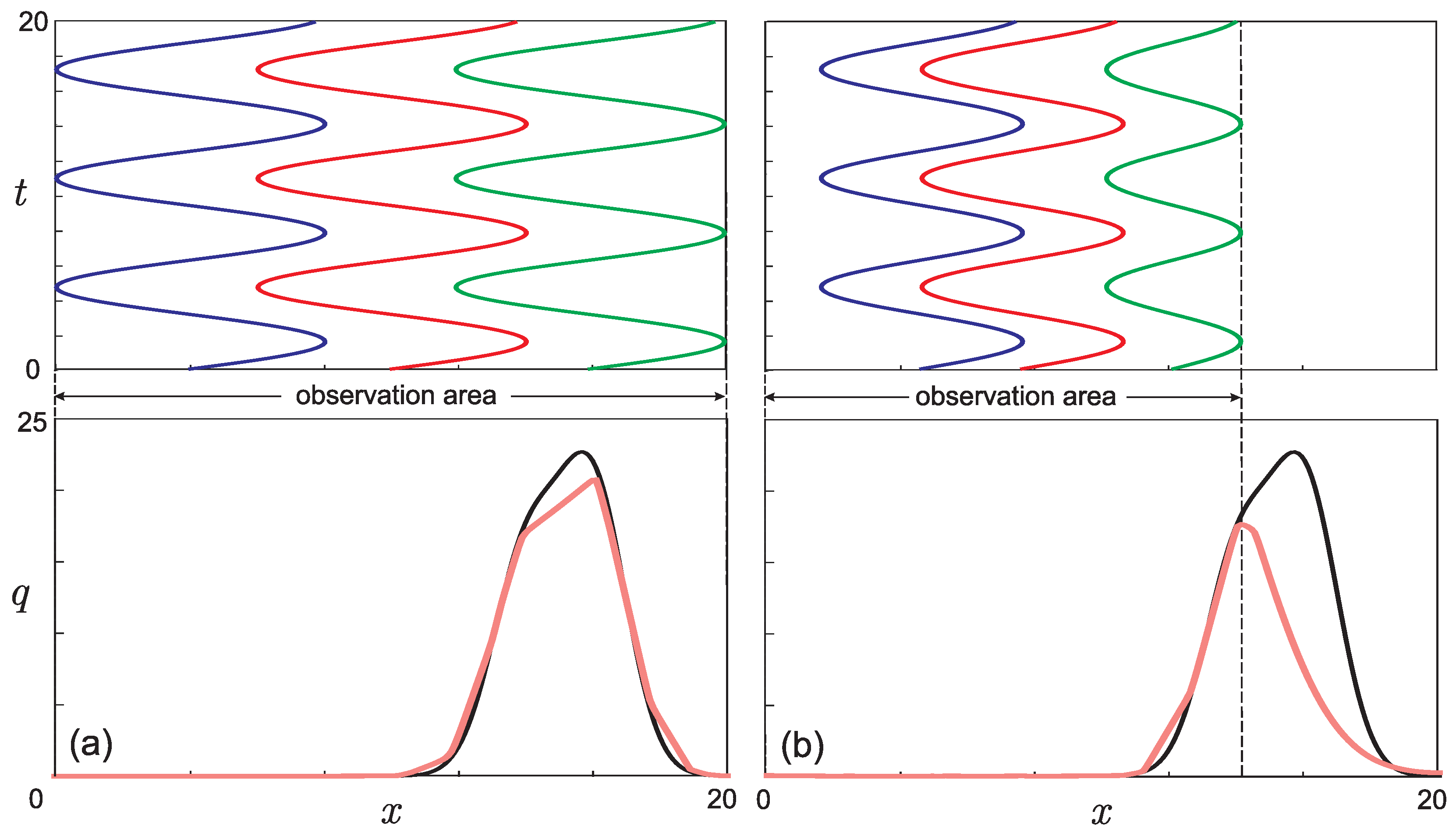
Figure 4a shows the curves (10) and the result of function q ( x ) q inv ( x ) retrieval for the specified model parameters. The curves (10) in the top picture well cover the region ( x , t ) [ 0 , 20 ] × [ 0 , 20 ] , and the solution q inv ( x ) reproduces the model function q model ( x ) over the entire area under consideration.

3.2. A Model Example with a Set of Curves That Fractionally Cover the Region of the Unknown Function q ( x ) Definition

Now we consider a model example for the same set of parameters (9) as in the previous example, but with another set of curves:
f 1 1 ( t ) = 3 sin ( t ) + 5 , f 1 2 ( t ) = 3 sin ( t ) + 8 , f 1 3 ( t ) = 2 sin ( t ) + 12.5 .
For the specified set of parameters, we have simulated the functions f 2 i ( t ) , i = 1 , I ¯ , I = 3 according to the algorithm described in Section 3.1.
The steepest descent method was implemented using uniform meshes (11) and (12) with N = 200 and M = 200 , the descent parameter β s = 3.5 × 10 3 , the regularization parameter α = 1 , the number of iterations of the gradient method S = 3000 , and the initial approximation q ( 0 ) ( x ) 0 . When solving the adjoint problem (7), the Formula (13) with ω = 0.01 was used.
Figure 4b shows the curves (14) and the result of the function q ( x ) q inv ( x ) retrieval for the specified model parameters. The curves (14) in the top picture cover only part of the region ( x , t ) [ 0 , 20 ] × [ 0 , 20 ] , and the solution q inv ( x ) reproduces the model function q model ( x ) quite well only in the area covered by the model curves (14).

3.3. Example of the Real Experimental Data Processing

Now we consider the inverse problem (3) and (4) for a set of parameters corresponding to the given biophysical model:
λ 1 = 27.17 , λ 2 = 0.99 , t 0 = 5 , L = 20 , T = 20 , γ ( x ) = k e b x k , k = 1.84835308 , b = 0.18203879 , B T * = 0.27 .
As additional information, we used the following arrays of experimental data from Table 1, Table 2 and Table 3 ( I = 3 ):
To process these experimental data, we interpolated the table values ( t e x p i , f 1 e x p i ) and ( t e x p i , f 2 e x p i ) , i = 1 , 3 ¯ , onto a uniform mesh (11) with a given number of intervals M. We have used the processed experimental data to numerically solve the original inverse problem by means of the steepest descent method.
The steepest descent method was implemented using uniform meshes (11) and (12) with N = 200 and M = 200 , the descent parameter β s = 2.5 × 10 3.5 , the regularization parameter α = 10 , the number of iterations of the gradient method S = 3000 , and the initial approximation q ( 0 ) ( x ) 0 . When solving the adjoint problem (7), the Formula (13) with ω = 0.01 was used.
Figure 5 shows the experimental sets of values f 1 e x p i ( t e x p i ) , i = 1 , 3 ¯ and the result of the function q ( x ) q inv ( x ) retrieval for the indicated experimental parameters.

4. Discussion

  • Each group of laboratory mice in the experiment described in [22] was kept in isolation and could be considered as an individual population. However, the experiment actually involved three pairs of parental mice, which can be considered one group of six mice at the initial time. The original goal of the work was to confirm the assumption that in each group of mice, the number of phenotypic differences in the first generation was different. If the initial pairs of laboratory mice in the experiment were identical, then the three different phenotypic curves shown in Figure 3b would not appear.
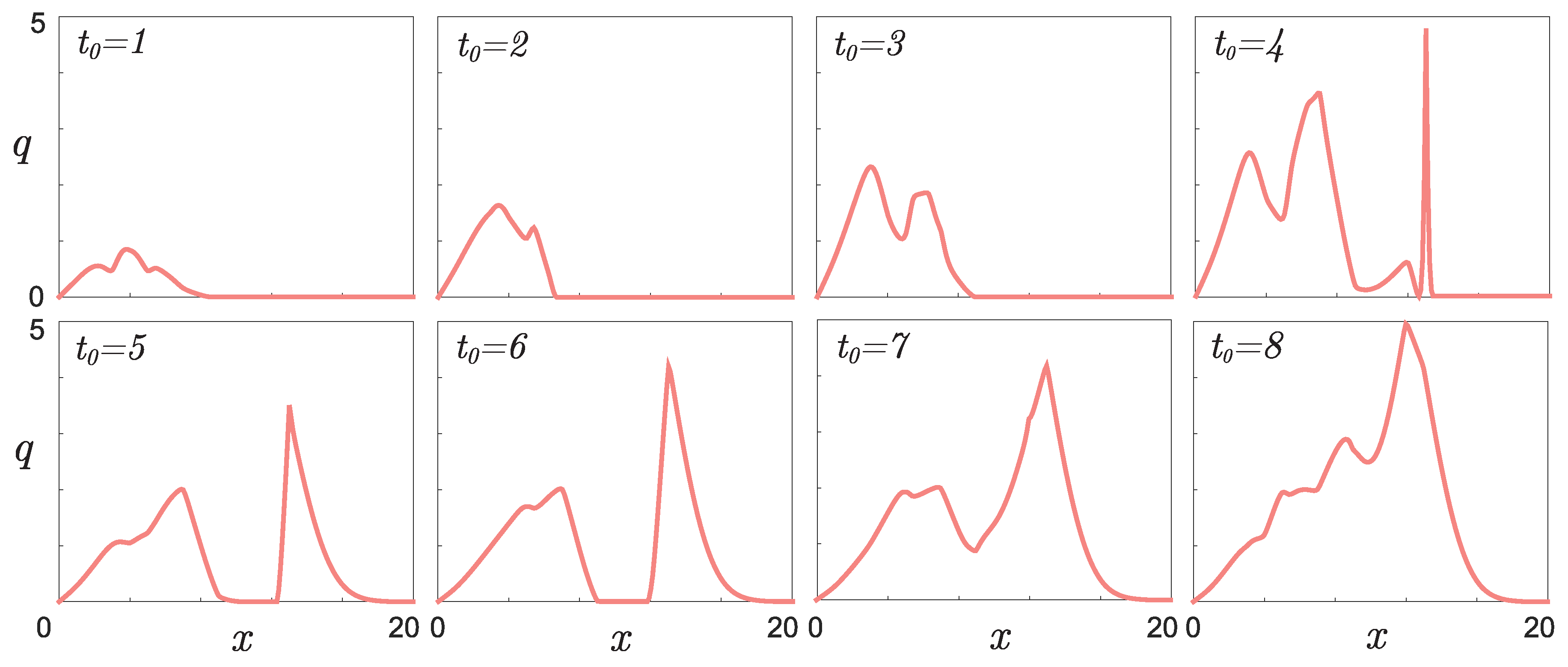
  • Figure 6 shows the result of the function retrieving that defines the initial phenotypic differences in the mouse population described in [22] for different values of parameter t 0 , which indicates the time for mutation accumulation to a number sufficient for the appearance of visible differences in individuals.
    From the form of the retrieved initial function, it follows that among the six initial mice, given t 0 4 , there is at least one individual phenotypically different from the others. For example, the green line in Figure 3b may correspond to a pair of “identical” parental mice that gave rise to a population in which visible differences appeared only in the fifth generation. However, if you take a couple of different mice, then a new mutant line will appear already in the second generation (red line). Apparently, the most realistic values are t 0 = 4 or t 0 = 5 , since with such a delay time, regardless of the number of individuals at the initial time, there are no more than two different phenotypic groups in the initial set of mice, as a result of which all initial individuals could be considered identical in the experiment.
  • The presence of a dip in the graphs of the retrieved initial data can be explained by the lack of points on the experimental graphs. Indirectly, this assumption is confirmed by the result of solving the model example presented in Figure 5: with a lack of input data, the initial curve is restored worse.
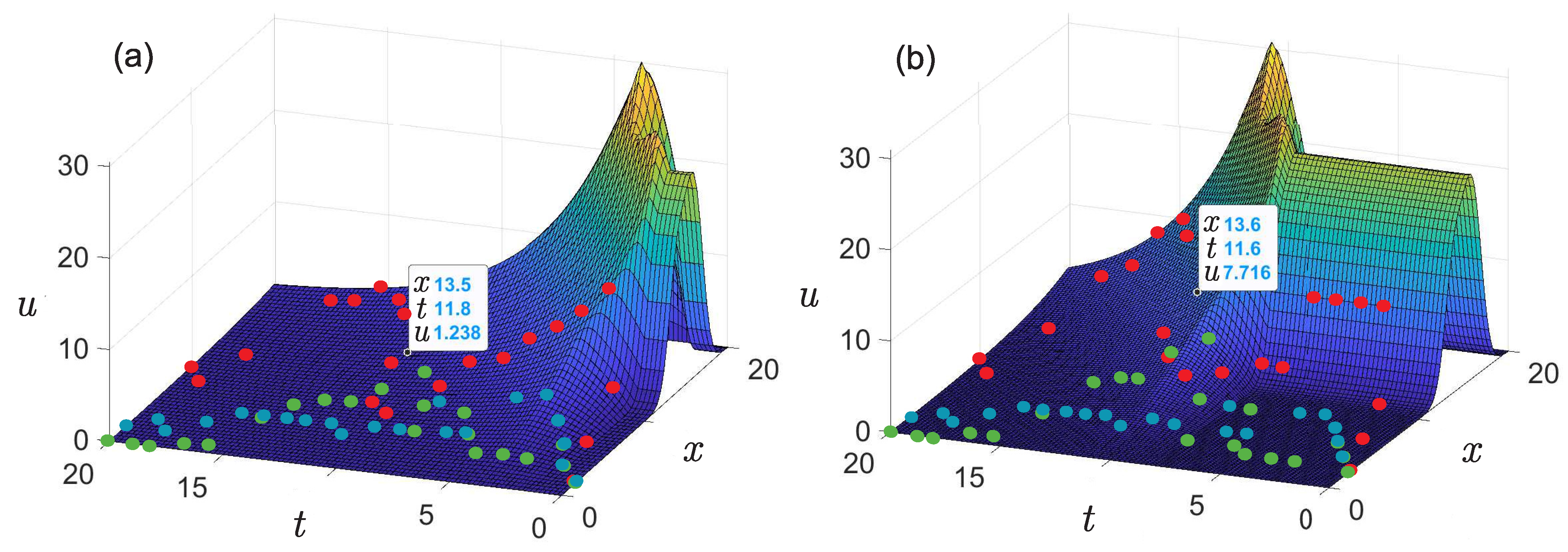
    The absence of a dip in the retrieved curve at t 0 = 8 is due to the fact that the function describing the solution of the direct problem with such a time delay lies in that region of the phase space ( x , t ) (see Figure 3a) for which there is sufficient data. This assumption can also be illustrated on three-dimensional graphs of the solution u ( x , t ) to the direct problem (Figure 7). The blue, red, and green points marked on the graphs correspond to the known coordinates ( x , t ) of the nodes on the phase curves f 1 e x p i , i = 1 , 3 ¯ , indicated, respectively, in Table 1, Table 2 and Table 3. The graph in Figure 7a corresponds to t 0 = 1 . It can be seen that at most points where the experimental data are given, the value of the function u ( x , t ) is almost equal to zero. Therefore, the initial function is poorly restored from these data (see Figure 6 for t 0 = 1 ). The graph in Figure 7b corresponds to t 0 = 8 . Practically all nodal points fall into the range of nonzero values of the function u ( x , t ) . The initial function is restored without “dips” (see Figure 6 for t 0 = 8 ). However, this result cannot be considered physically substantiated since it yields to the conclusion that initially there were too many phenotypically different mice in the population, which contradicts the large delay in mutation accumulation.
  • The way to improve the retrieval quality is to increase the number of experimental curves in the coverage area.

5. Conclusions

This paper presents an algorithm for retrieving the initial conditions of the initial-boundary value problem for the diffusion equation with a priori information on the values of the direct problem solution on several curves in phase spaces.
Despite the small amount of known data, we managed to make an assumption regarding the time of the mutations’ accumulation to a number sufficient for the appearance of visible differences in individuals in the mouse population and found that the initial set of mice in the experiment described in [22] already consisted of at least two phenotypically different groups of mice. This result was possible thanks to the active development of methods for solving coefficient inverse problems for partial differential equations with data on curves inside the domain (see [34,35,36,37,38,39]).
The results obtained in the course of solving the inverse problem can be used in the analysis of the dynamics of congenital diseases.

Author Contributions

Conceptualization, A.S., N.L. and D.L.; methodology, D.L. and M.S.; software, R.A.; validation, A.S., N.L. and R.A.; formal analysis, A.S. and N.L.; investigation, A.S.; writing—original draft preparation, R.A., N.L. and A.S.; writing—review and editing, D.L. and M.S.; visualization, D.L.; supervision, N.L.; project administration, N.L.; funding acquisition, N.L. All authors have read and agreed to the published version of the manuscript.

Funding

This research was funded by Russian Science Foundation (project 23-11-00069).

Data Availability Statement

Not applicable.

Acknowledgments

The team of authors thanks the Foundation for the Development of Theoretical Physics and Mathematics “BASIS” for supporting the young scientist Raul Argun.

Conflicts of Interest

The authors declare no conflict of interest.

Appendix A. Obtaining Additional Information for Solving the Inverse Problem from Experimental Data (Tables in Appendix Section Were Obtained with the Participation of Anastasia Garayeva)

Since the article [22] does not contain data on the number of mice in each generation, to obtain the dependence of the number of mice (N) on the generation number (n) (Figure 3a) and the functions f 1 i , i = 1 , 2.3 in Table 1, Table 2 and Table 3, we used the equation [21]:
[ N ( n ) ] = N ( n 1 ) r 3 N ( n 1 ) + r 4 N ( n 1 ) ,
where r 3 is a mortality rate constant and r 4 is a birth rate constant. Square brackets mean rounding to the nearest integer.
Mice mortality and birth rate constants were determined using experimental data from [22]. The results are summarized in Table A1. All values are calculated for the total number of mutant mice in all three mutant groups. Column I shows the generation numbers. Column II contains information from [22] on the mice’s survival (the proportion of mice that survived to a reproductive age of 8 weeks). Column III contains information about the average number of offspring per mating. The birth rate constant ( r 4 , column IV) is defined as the product of survival (column II) and the number of offspring per mating (column III). The mortality rate constant ( r 3 , column V) is defined as the difference between the number of offspring per mating (column III) and the birth rate constant r 4 , and means the proportion of offspring that did not survive to puberty.
Table A1. The data to obtain mice mortality and birth rate constants.
IIIIIIIVV
GenerationMice SurvivalOffspring per Mating r 4 r 3
0–20.672.641.770.87
3–60.511.310.66810.6419
7–120.490.960.47040.4896
Table A2 summarizes the information needed to plot the curves in Figure 3a. Column I contains the generation number (n). Column II contains the total number of mutant mice in three groups (N) calculated from equation (A1). Columns III, IV, and V indicate the number of phenotypic differences in each of the mutant groups, depending on the generation. They contain the same values f 2 i , i = 1 , 2 , 3 , as in Table 1, Table 2 and Table 3, respectively. Obviously, these values coincide with the number of groups of phenotypically indistinguishable individuals in each generation. Column VII gives the average number of individuals per group of phenotypically indistinguishable mice. By multiplying this number by the number of phenotypic differences in a given generation for the respective group (columns III, IV, V), the number of mice in each group can be calculated. These values for each of the three groups are presented in columns VIII, IX, and X. Those calculated values that turned out to be less than the number of groups of phenotypically identical mice indicated in columns III, IV, and V are highlighted in red. Obviously, the calculation in this case gave underestimated results. Therefore, when compiling the sets of values f 1 i , i = 1 , 2 , 3 , respectively, in Table 1, Table 2 and Table 3, we replaced the calculated values with the number of groups of identical mice (values highlighted in blue), since the average number of mice in each such group does not exceed 1 (see values in column VII).
Table A2. The data to obtain the number of mice in each generation: values f 1 i , i = 1 , 2 , 3 , respectively, in Table 1, Table 2 and Table 3 for graphs in Figure 3a. Red colors marks the underestimated values, blue coloured are the values with which we replaced the underestimated ones in the Table 1, Table 2 and Table 3.
IIIIIIIVVVIVIIVIIIIXX
nN f 2 1 f 2 2 f 2 3 F = f 2 1 + f 2 2 + f 2 3 N / F f 1 1 = ( N / F ) f 2 1 f 1 2 = ( N / F ) f 2 2 f 1 3 = ( N / F ) f 2 3
0611132222
11112142.85363
22212145.45115
32224173.176133
42324173.257133
52324173.347133
62425292.665135
724253102.355127
823352102.37125
923365141.615108
1022469191.175711
1122479201.094810
12215129260.824107
13215189320.653125
14215198320.643125
15205205300.673133
16205191250.794151
17194191230.843151
18192130150.842110
191926081.55390
201814052.432100

References

  1. Peisajovich, S.; Garbarino, J.; Wei, P.; Lim, W. Rapid Diversification of Cell Signaling Phenotypes by Modular Domain Recombination. Science 2010, 328, 368–372. [Google Scholar] [CrossRef] [PubMed] [Green Version]
  2. Showalter, A.; Tsai, M. A reexamination of the nucleotide incorporation fidelity of DNA polymerases. Biochemistry 2002, 41, 10571–10576. [Google Scholar] [CrossRef]
  3. Echols, H.; Goodman, M.F. Fidelity mechanisms in DNA replication. Annu. Rev. Biochem. 1991, 60, 477–511. [Google Scholar] [CrossRef] [PubMed]
  4. Kunkel, T. Evolving Views of DNA Replication (In)Fidelity. Cold Spring Harb. Symp. Quant. Biol. 2009, 74, 91–101. [Google Scholar] [CrossRef]
  5. Kunkel, T.; Burgers, P. Dividing the workload at a eukaryotic replication fork. Trends Cell Biol. 2008, 18, 521–527. [Google Scholar] [CrossRef] [PubMed] [Green Version]
  6. McCulloch, S.; Kunkel, T. The fidelity of DNA synthesis by eukaryotic replicative and translesion synthesis polymerases. Cell Res. 2008, 18, 148–161. [Google Scholar] [CrossRef] [Green Version]
  7. Charles, J.S. Quantifying the contributions of base selectivity, proofreading and mismatch repair to nuclear DNA replication in Saccharomyces cerevisiae. DNA Repair 2015, 31, 41–51. [Google Scholar] [CrossRef] [Green Version]
  8. Alberts, B. Molecular Biology of the Cell; Garland Science, Taylor and Francis Group: New York, NY, USA, 2015. [Google Scholar]
  9. Burgers, P. Polymerase Dynamics at the Eukaryotic DNA Replication Fork. J. Biol. Chem. 2009, 284, 4041–4045. [Google Scholar] [CrossRef] [Green Version]
  10. Prindle, M.; Loeb, L. DNA Polymerase Delta in Dna Replication and Genome Maintenance. Environ. Mol. Mutagen. 2012, 53, 666–682. [Google Scholar] [CrossRef] [Green Version]
  11. Johnson, R.; Klassen, R.; Prakash, L.; Prakash, S. A Major Role of DNA Polymerase δ in Replication of Both the Leading and Lagging DNA Strands. Mol. Cell 2015, 59, 163–175. [Google Scholar] [CrossRef] [Green Version]
  12. Lujan, S.; Williams, J.; Kunkela, T. DNA polymerases divide the labor of genome replication. Trends Cell Biol. 2016, 26, 640–654. [Google Scholar] [CrossRef] [PubMed] [Green Version]
  13. Ma, X.; Dong, L.; Liu, X.; Ou, K.; Yang, L. POLE/POLD1 mutation and tumor immunotherapy. J. Exp. Clin. Cancer Res. 2022, 41, 216. [Google Scholar] [CrossRef] [PubMed]
  14. Gola, M.; Stefaniak, P.; Godlewski, J.; Jereczek-Fossa, B.; Starzyńska, A. Prospects of POLD1 in Human Cancers: A Review. Cancers 2023, 15, 1905. [Google Scholar] [CrossRef] [PubMed]
  15. Godlewski, J.; Stefaniak, P.; Kiezun, J.; Krazinski, B. DNA Polymerase Delta 1 Catalytic Subunit (POLD1) as a Prognostic Factor in Clear Cell Renal Cell Carcinoma Patients. In Vivo 2022, 36, 1188–1194. [Google Scholar] [CrossRef] [PubMed]
  16. Brunet, E.; Rouzine, I.; Wilke, C. The stochastic edge in adaptive evolution. Genetics 2008, 179, 603–620. [Google Scholar] [CrossRef] [PubMed] [Green Version]
  17. Hallatschek, O.; Geyrhofer, L. Collective fluctuations in the dynamics of adaptation and other traveling waves. Genetics 2016, 202, 1201–1227. [Google Scholar] [CrossRef]
  18. Travis, J.; Travis, E. Mutator dynamics in fluctuating environments. Proc. Biol. Sci. 2002, 269, 591–597. [Google Scholar] [CrossRef]
  19. Good, B.; Desai, M. Evolution of Mutation Rates in Rapidly Adapting Asexual Populations. Genetics 2016, 204, 1249–1266. [Google Scholar] [CrossRef]
  20. Desai, M.; Fisher, D. The balance between mutators and nonmutators in asexual populations. Genetics 2011, 188, 997–1014. [Google Scholar] [CrossRef] [Green Version]
  21. Garaeva, A.; Sidorova, A.; Levashova, N.; Tverdislov, V. Self-Organized Criticality in the Autowave Model of Speciation. Mosc. Univ. Phys. Bull. 2020, 75, 398–408. [Google Scholar] [CrossRef]
  22. Uchimura, A.; Higuchi, M.; Minakuchi, Y.; Ohno, M.; Toyoda, A.; Fujiyama, A.; Miura, I.; Wakana, S.; Nishino, J.; Yag, T. Germline mutation rates and the long-term phenotypic effects of mutation accumulation in wild-type laboratory mice and mutator mice. Genome Res. 2015, 25, 1125–1134. [Google Scholar] [CrossRef] [Green Version]
  23. Lynch, M.; Ackerman, M.; Gout, J.; Long, H.; Sung, W.; Thomas, W.; Foster, P. Genetic drift, selection and the evolution of the mutation rate. Nat. Rev. Genet. 2016, 17, 704–714. [Google Scholar] [CrossRef] [PubMed]
  24. Butuzov, V.; Nefedov, N.; Schneider, K. Singularly perturbed boundary value problems for systems of Tikhonov’s type in case of exchange of stabilities. J. Differ. Equ. 1999, 159, 427–446. [Google Scholar] [CrossRef] [Green Version]
  25. Butuzov, V.; Nefedov, N.; Schneider, K. On a singularly perturbed system of parabolic equations in the case of intersecting roots of the degenerate equation. Comput. Math. Math. Phys. 2002, 42, 176–187. [Google Scholar]
  26. Tikhonov, A.N.; Goncharsky, A.V.; Stepanov, V.V.; Yagola, A.G. Numerical Methods for the Solution of Ill-Posed Problems; Kluwer Academic Publishers: Dordrecht, The Netherlands, 1995. [Google Scholar]
  27. Haskell, B.C. The method of steepest descent for non-linear minimization problems. Q. Appl. Math. 1944, 2, 258–261. [Google Scholar] [CrossRef] [Green Version]
  28. Kabanikhin, S.; Shishlenin, M. Quasi-solution in inverse coefficient problems. J. Inverse Ill-Posed Probl. 2008, 16, 705–713. [Google Scholar] [CrossRef]
  29. Vasin, V.; Eremin, I. Operators and Iterative Processes of Fejér Type: Theory and Applications; Walter de Gruyter: Berlin, Germany, 2009. [Google Scholar]
  30. Klyuchinskiy, D.; Novikov, N.; Shishlenin, M. CPU-time and RAM memory optimization for solving dynamic inverse problems using gradient-based approach. J. Comput. Phys. 2021, 439, 110374. [Google Scholar] [CrossRef]
  31. Hairer, E.; Wanner, G. Solving Ordinary Differential Equations II. Stiff and Differential-Algebraic Problems; Springer: Berlin/Heidelberg, Germany, 1996. [Google Scholar]
  32. Rosenbrock, H. Some general implicit processes for the numerical solution of differential equations. Comput. J. 1963, 5, 329–330. [Google Scholar] [CrossRef] [Green Version]
  33. Wen, X. High order numerical methods to a type of delta function integrals. J. Comput. Phys. 2007, 226, 1952–1967. [Google Scholar] [CrossRef]
  34. Lukyanenko, D.; Borzunov, A.; Shishlenin, M. Solving coefficient inverse problems for nonlinear singularly perturbed equations of the reaction-diffusion-advection type with data on the position of a reaction front. Commun. Nonlinear Sci. Numer. Simul. 2021, 99, 105824. [Google Scholar] [CrossRef]
  35. Lukyanenko, D.; Yeleskina, T.; Prigorniy, I.; Isaev, T.; Borzunov, A.; Shishlenin, M. Inverse problem of recovering the initial condition for a nonlinear equation of the reaction-diffusion-advection type by data given on the position of a reaction front with a time delay. Mathematics 2021, 9, 342. [Google Scholar] [CrossRef]
  36. Levashova, N.; Gorbachev, A.; Argun, R.; Lukyanenko, D. The problem of the non-uniqueness of the solution to the inverse problem of recovering the symmetric states of a bistable medium with data on the position of an autowave front. Symmetry 2021, 13, 680. [Google Scholar] [CrossRef]
  37. Argun, R.; Gorbachev, A.; Lukyanenko, D.; Shishlenin, M. On some features of the numerical solving of coefficient inverse problems for an equation of the reaction-diffusion-advection-type with data on the position of a reaction front. Mathematics 2021, 9, 2894. [Google Scholar] [CrossRef]
  38. Argun, R.; Gorbachev, A.; Levashova, N.; Lukyanenko, D. Inverse problem for an equation of the reaction-diffusion-advection type with data on the position of a reaction front: Features of the solution in the case of a nonlinear integral equation in a reduced statement. Mathematics 2021, 9, 2342. [Google Scholar] [CrossRef]
  39. Isakov, V.; Kabanikhin, S.; Shananin, A.; Shishlenin, M.; Zhang, S. Algorithm for determining the volatility function in the Black-Scholes model. Comput. Math. Math. Phys. 2019, 59, 1753–1758. [Google Scholar] [CrossRef]
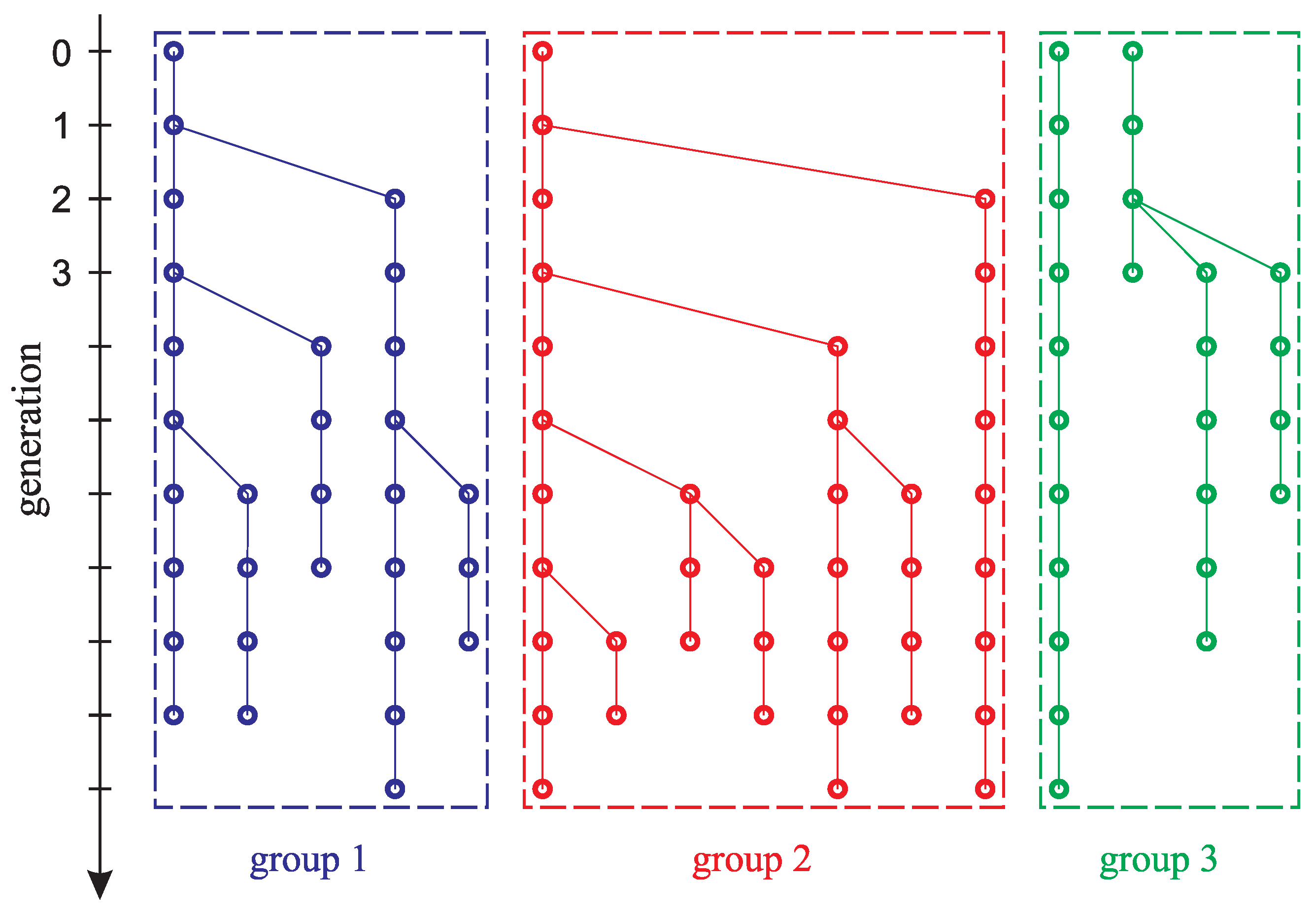
Figure 1. Schematic representation of the mutant lines’ appearance. Each isolated group of mice is marked with a separate color. Each circle represents a group of phenotypically identical individuals. Circles at the same horizontal level correspond to the same generation in the mouse population. The lines connecting the circles represent the transition from the generation of parents to the generation of children. Each mutant line on the scheme is traced as a set of circles connected by vertical lines. Each line branching off to the side means a transition from parents to descendants phenotypically different from the latter.
Mathematics 11 03180 g001
Figure 2. Illustration of the direct problem solution change over time: the numerical solution u ( x , t ) (thick red line), the function u 1 ( x , t ) (solid black line), and the function u 2 ( x , t ) (dashed black line).
Mathematics 11 03180 g002
Figure 3. The graphs obtained from experimental results [22]: (a) dynamics of the number of individuals x in each of the three mutant groups of mice over generations (t); and (b) dynamics in the phenotypic differences (adapted from [21]) (u) for the three mutant groups of mice over generations t. Different mutant groups are marked with different colors.
Mathematics 11 03180 g003
Figure 4. Top pictures: (a) model curves (10): f 1 1 ( t ) (blue line), f 1 2 ( t ) (red line), f 1 3 ( t ) (green line); and (b) model curves (14): f 1 1 ( t ) (blue line), f 1 2 ( t ) (red line), f 1 3 ( t ) (green line). Bottom pictures: the model function q model ( x ) (black line) and the retrieved function q inv ( x ) (red line) for the parameter set (9) and (10).
Mathematics 11 03180 g004
Figure 5. Top picture: experimental curves drawn with the sets of values f 1 e x p 1 ( t e x p ) , (Table 1, blue line), f 1 e x p 2 ( t e x p ) , (Table 2, red line), and f 1 e x p 3 ( t e x p ) , (Table 3, green line). Bottom picture: the retrieved function q inv ( x ) for the experimental parameter set (15).
Mathematics 11 03180 g005
Figure 6. Results of retrieving the initial conditions of the problem (6) with different delay times.
Mathematics 11 03180 g006
Figure 7. Graph of the direct problem solution, u ( x , t ) . The points on the graph correspond to the known coordinates ( x , t ) of nodes on the phase curves f 1 e x p 1 (Table 1, blue points), f 1 e x p 2 (Table 2, red points), f 1 e x p 3 (Table 3, green points). (a) t 0 = 1 . (b) t 0 = 8 . The coordinates in squares show the difference in the values of the function u ( x , t ) at the reference points for different t 0 .
Mathematics 11 03180 g007
Table 1. Sets of experimental values for plotting the curves f 1 1 ( t ) and f 2 1 ( t ) (blue color in Figure 3).
t e x p 1 01234567891011121314151617181920
f 1 e x p 1 235677557554555554232
f 2 e x p 1 111222223344555554221
Table 2. Sets of experimental values for plotting the curves f 1 2 ( t ) and f 2 2 ( t ) (red color in Figure 3).
t e x p 2 01234567891011121314151617181920
f 1 e x p 2 2611131313131212107812181920191913910
f 2 e x p 2 1224445556671218192019191364
Table 3. Sets of experimental values for plotting the curves f 1 3 ( t ) and f 2 3 ( t ) (green color in Figure 3).
t e x p 3 01234567891011121314151617181920
f 1 e x p 3 23533357581110998511000
f 2 e x p 3 111111232599998511000
Disclaimer/Publisher’s Note: The statements, opinions and data contained in all publications are solely those of the individual author(s) and contributor(s) and not of MDPI and/or the editor(s). MDPI and/or the editor(s) disclaim responsibility for any injury to people or property resulting from any ideas, methods, instructions or products referred to in the content.