Article

Effects of Exploration Weight and Overtuned Kernel Parameters on Gaussian Process-Based Bayesian Optimization Search Performance

College of Industrial Technology, Nihon University, 1-2-1, Izumi, Narashino, Chiba 275-8575, Japan
Mathematics 2023, 11(14), 3067; https://doi.org/10.3390/math11143067
Submission received: 7 June 2023 / Revised: 4 July 2023 / Accepted: 7 July 2023 / Published: 11 July 2023

Abstract

:
Gaussian process-based Bayesian optimization (GPBO) is used to search parameters in machine learning, material design, etc. It is a method for finding optimal solutions in a search space through the following four procedures. (1) Develop a Gaussian process regression (GPR) model using observed data. (2) The GPR model is used to obtain the estimated mean and estimated variance for the search space. (3) The point where the sum of the estimated mean and the weighted estimated variance (upper confidence bound, UCB) is largest is the next search point (in the case of a maximum search). (4) Repeat the above procedures. Thus, the generalization performance of the GPR is directly related to the search performance of the GPBO. In procedure (1), the kernel parameters (KPs) of the GPR are tuned via gradient descent (GD) using the log-likelihood as the objective function. However, if the number of iterations of the GD is too high, there is a risk that the KPs will overfit the observed data. In this case, because the estimated mean and variance output by the GPR model are inappropriate, the next search point cannot be properly determined. Therefore, overtuned KPs degrade the GPBO search performance. However, this negative effect can be mitigated by changing the parameters of the GPBO. We focus on the weight of the estimated variances (exploration weight) of the UCB as one of these parameters. In a GPBO with a large exploration weight, the observed data appear in various regions in the search space. If the KP is tuned using such data, the GPR model can estimate the diverse regions somewhat correctly, even if the KP overfits the observed data, i.e., the negative effect of overtuned KPs on the GPR is mitigated by setting a larger exploration weight for the UCB. This suggests that the negative effect of overtuned KPs on the GPBO search performance may be related to the UCB exploration weight. In the present study, this hypothesis was tested using simple numerical simulations. Specifically, GPBO was applied to a simple black-box function with two optimal solutions. As parameters of GPBO, we set the number of KP iterations of GD in the range of 0–500 and the exploration weight as { 1 , 5 } . The number of KP iterations expresses the degree of overtuning, and the exploration weight expresses the strength of the GPBO search. The results indicate that, in the overtuned KP situation, GPBO with a larger exploration weight has better search performance. This suggests that, when searching for solutions with a small GPBO exploration weight, one must be careful about overtuning KPs. The findings of this study are useful for successful exploration with GPBO in all situations where it is used, e.g., machine learning hyperparameter tuning.

1. Introduction

Gaussian process-based Bayesian optimization (GPBO) optimizes black-box functions and is adopted to save time and/or reduce costs. For example, it is used for concrete design [1,2], material design [3,4,5], and tuning hyperparameters in machine learning (for support vector machines [6,7,8], random forest models [9,10] and neural networks [9,11,12], etc.). Appropriate parameters can be obtained more rapidly using GPBO compared with simple methods such as grid search. For example, Wu et al. [9] reported that the computation time of hyperparameter tuning in machine learning can be reduced significantly using GPBO. Snoek et al. [11] reported that when GPBO was used for tuning, the developed convolutional neural networks had higher generalization scores than networks with parameters tuned by an expert of machine learning.
To perform GPBO, a Gaussian process regression (GPR) model must be developed, which is computationally expensive. The computational cost of the kernel inverse matrix required in GPBO is O ( n 3 ) for a data size of n [13]. Due to the fact that n increases with each successive GPBO iteration, the computational cost increases. Therefore, sparse matrix methods [13,14,15,16] and mini-batch methods [17] have been proposed for reducing the computational cost.
In the log-likelihood-based objective function, the kernel inverse matrix is used to tune the hyperparameters of the GPR model [18]. Gradient-based methods [17,19,20], evolutionary algorithms [21,22], and Markov chain Monte Carlo methods [23] have been adopted for hyperparameter tuning of the GPR model. Cross-validation [18] is adopted for tuning the kernel parameters (KPs) to avoid overfitting to the observed data. However, because the size of the observed data gradually increases, performing cross-validation at the beginning of GPBO is difficult. Therefore, we cannot perform cross-validation at the beginning of GPBO to tune the hyperparameters of the GPR model. Moreover, cross-validation increases the computational cost [18].
In the early stages of GPBO, the sample size is insufficient. Additionally, it is difficult to properly tune a GPR model by a small sample size [24,25]. Therefore, consider the situation wherein the KPs are tuned using all samples instead of using a method that reduces the number of data, such as cross-validation. In this case, because there are no data for validation, it is not known to what extent the KPs should be fitted to the observed data. Thus, there is a risk of overtuning the GPR model. Overtuned GPR models can correctly estimate observed regions but cannot properly estimate unobserved regions [26]. GPBO is an algorithm that searches for the optimal solution in unobserved regions. Therefore, if unobserved areas cannot be correctly estimated, a proper search cannot be performed. From this viewpoint, the search performance of Bayesian optimization using an overfitted GPR model is expected to be poor.
The negative effect of overtuned KPs on the search performance depends on other parameters of GPBO. We focus on the exploration weight of the upper confidence bound (UCB) [27,28], which is a GPBO parameter. Generally, when the exploration weight is set to a large value, the next search point tends to be selected from regions with insufficient observations; therefore, the observed samples appear in various areas. In this case, even if the KPs are overfitted to the observed samples, the GPR model can correctly estimate the various input domains. In contrast, with a small exploration weight, because the observed samples appear in only limited regions, the overfitted GPR model only estimates limited regions; therefore, its generalization score is worse.
This implies that the risk of overtuned KPs degrading the search performance depends on the exploration weight. We verified this hypothesis by analyzing the relationships among the overtuned KPs, exploration weight, and GPBO search performance. The results indicated that, for GPBO, more attention must be paid to the overtuning of the KPs in the case of smaller exploration weights. Additionally, it is necessary to pay attention to avoid overtuning KPs when searching for the solution via GPBO with a small exploration weight. These findings are useful for successful exploration with GPBO in all situations where it is used, e.g., hyperparameter tuning in machine learning.
As indicated by previous studies [21,24,25], the likelihood function in GPR may have multiple minimal solutions, making it difficult to find a globally optimal solution. Therefore, we focused on gradient descent (GD), which can rapidly obtain a local minimal solution, as a method for tuning the KPs. This method is widely used for tuning the KPs of GPR models [17,19,20].

2. Gaussian Process-Based Bayesian Optimization

2.1. Surrogate Model

In this study, we use the GPR model as a surrogate model for Bayesian optimization, which we call GPBO. This method outputs the estimated average and variance by assuming a Gaussian distribution from the dataset D consisting of pairs of observed input and output values.
Here, the output value y is obtained as
y = f ( x ) + ϵ ,
where x = [ x 1 x D ] is the D-dimensional input vector, f ( x ) is a black-box function, and ϵ denotes observation noise. In addition, we consider a situation in which a dataset
D = { ( x n , y n ) | n = 1 , , N }
is collected via N observations. In the case of GPR, assuming that the average of y is zero, the average and variance values of the output y for the new input data x are given as follows:
E [ y | x , D , θ ] = k ( θ ) K ( θ ) 1 y ,
V [ y | x , D , θ ] = k ( θ ) k ( θ ) K ( θ ) 1 k ( θ )
where y = [ y 1 y N ] . K ( θ ) is a kernel matrix defined as follows:
K ( θ ) = k ( x i , x j ; θ ) R > 0 N × N
where k ( x i , x j ; θ ) denotes the kernel function. For Gaussian kernels, the kernel function is defined as
k ( x i , x j ; θ ) = θ 1 exp | | x i x j | | 2 2 θ 2 + θ 3 δ ( i , j ) , δ ( i , j ) = 0 , i j 1 , i = j , θ R > 0 3
where θ = ( θ 1 , θ 2 , θ 3 ) is a vector comprising three KPs. Due to the fact that the estimation accuracy depends on the KPs, appropriate tuning is important. k ( θ ) and k ( θ ) are the kernels related to the observed samples x i and new sample x , respectively, and are defined as follows:
k ( θ ) = k ( x , x ; θ ) , k ( θ ) = k ( x i , x ; θ ) R > 0 N .

2.2. Tuning Kernel Parameters

As stated in the Introduction, the KP vector θ is tuned using GD. Due to the fact that the θ that maximizes the generation probability of the observed output y is desirable, using the log-likelihood, the objective function L is defined as
L ( θ ) = log p ( y | θ ) = log N ( 0 , K ( θ ) ) = log 1 ( 2 π ) N | K ( θ ) | exp 1 2 y K ( θ ) 1 y log | K ( θ ) | y K ( θ ) 1 y .
We assume that p ( y | θ ) is a Gaussian distribution consisting of the average 0 and the covariance matrix K ( θ ) . When we adopt the gradient method for the objective function, θ may be negative. Due to the fact that the Gaussian KP θ requires a plus (see Equation (6)), θ is redefined as follows:
θ = g ( θ ) = exp ( θ ) , θ = [ θ 1 θ 2 θ 3 ]
where the map g is
g : R 3 R > 0 3 .
Therefore, when the gradient method is run as the search target θ and the obtained parameter is transformed into θ using Equation (9), θ will certainly be positive. Therefore, we use the update equation for the KPs, as follows:
θ ( t g + 1 ) = θ ( t g ) + γ L exp ( θ ( t g ) )
where t g represents the iteration count, θ ( t g ) is the t g -th specific value of θ , and γ represents the learning rate. This partial differentiation is as follows:
L exp ( θ ) = tr K ( exp ( θ ) ) 1 K ( exp ( θ ) ) + K ( exp ( θ ) ) 1 y K ( exp ( θ ) ) K ( exp ( θ ) ) 1 y .
Due to the fact that K is the matrix consisting of kernel functions, i.e., K ( exp ( θ ) ) , the partial derivative of k ( x i , x j ; exp ( θ ) ) with respect to θ 1 , θ 2 , θ 3 is required, i.e.,
k ( x i , x j ; exp ( θ ) ) θ 1 = exp ( θ 1 ) exp | | x i x j | | 2 2 exp ( θ 2 ) ,
k ( x i , x j ; exp ( θ ) ) θ 2 = exp ( θ 1 ) exp ( θ 2 ) | | x i x j | | 2 2 exp | | x i x j | | 2 2 exp ( θ 2 ) ,
k ( x i , x j ; exp ( θ ) ) θ 3 = exp ( θ 3 ) δ ( i , j ) .
This calculation technique was described by Mochihashi et al. [29].
After the parameter is updated T g times, we obtain θ ( T g ) . Substituting this into Equation (9) yields the tuned KP θ ( T g ) . According to Equation (10), the obtained parameter θ ( T g ) satisfies the condition of R > 0 3 .

2.3. Optimization Algorithm for Experiments

Using Equations (3) and (4), the acquisition function of GPBO is defined as
A ( x ; β , θ ) = E [ y | x , D , θ ] + β V [ y | x , D , θ ]
and it is called the UCB [27,28]. Here, with N observed samples, the N + 1 -th (next) observation sample is determined as follows:
x N + 1 = argmax x Ψ A ( x ; β , θ ) ,
y N + 1 = f ( x N + 1 ) + ϵ
where Ψ represents the domain of the input x . The second term of the acquisition function, which is defined in Equation (16), controls the search weight. When β is set to a large value, exploration is emphasized. Subsequently, the observation dataset is updated as
D = D { ( x N + 1 , y N + 1 ) } .
By performing this process T b times, we obtain the maximum value y max and the approximate solution x max as follows:
y max = max D y , x max = argmax x D x D y
where D y and D x are the sets consisting of the output and input values, respectively, of the set D . This procedure is presented in Algorithm 1.
Algorithm 1 Verification-targeted optimization algorithm
Input:

   Initial observation dataset D , maximum number of BO iterations T b ,

   maximum number of GD iterations T g , GD learning rate γ , exploration weight β ,

   black-box function f ( x ) , observation noise ϵ ,

   search space Ψ , initial KP θ ( 0 ) = exp ( θ ( 0 ) )

Output:

   Solution x max and its value y max

................................................................................................................................................

1:
for  t b = 1 to T b  do
2:
   for  t g = 0 to T g 1  do
3:
      θ ( t g + 1 ) θ ( t g ) + γ L exp ( θ ( t g ) )
4:
   end for
5:
    θ ( T g ) exp θ ( T g )
6:
    x N + 1 argmax x Ψ A ( x ; β , θ ( T g ) )
7:
    y N + 1 f ( x N + 1 ) + ϵ
8:
    D D { ( x N + 1 , y N + 1 ) }
9:
end for
10:
y max max D y , x max argmax x D x D y
11:
return  x max , y max
................................................................................................................................................

Notes:
· Lines 2–4: Tuning the KPs via GD;
· Lines 6–8: Decisions regarding the next search point and observation;
· Lines 10–11: Obtain an approximate solution.
“GD”: gradient descent, “BO”: Bayesian optimization

2.4. Indices

The GPBO search performance depends on the training and generalization errors of the surrogate model. Therefore, the training and generalization errors are, respectively, defined as
E t ( θ ) = 1 N n = 1 N y n E [ y n | x n , D , θ ] 2 ,
E v ( θ ) = 1 | Ψ | x Ψ f ( x ) E [ y | x , D , θ ] 2 .
Moreover, the GPBO search performance depends on whether the next search point x N + 1 and past observed points x 1 , , x N are close, i.e., if the search is performed only near past observation points, the search performance is poor. Therefore, we determine whether they are close to each other as follows:
min { | | x N + 1 x n | | 2 | n = 1 , , N } < ω
where ω denotes the threshold value. When the minimum distance on the left side is less than ω , the next search point x N + 1 is close to the previously observed points x 1 , , x N .
Furthermore, whether the KP vector θ ( T g ) obtained as T g times GD has converged is determined as follows:
| | θ ( T g ) θ ( T g 1 ) | | 2 | | θ ( T g 1 ) | | 2 < τ
where τ is the threshold for the convergence criterion. The term on the left side is called the “relative change in parameters,” and it is widely used as a convergence criterion [30,31,32].

3. Experiments

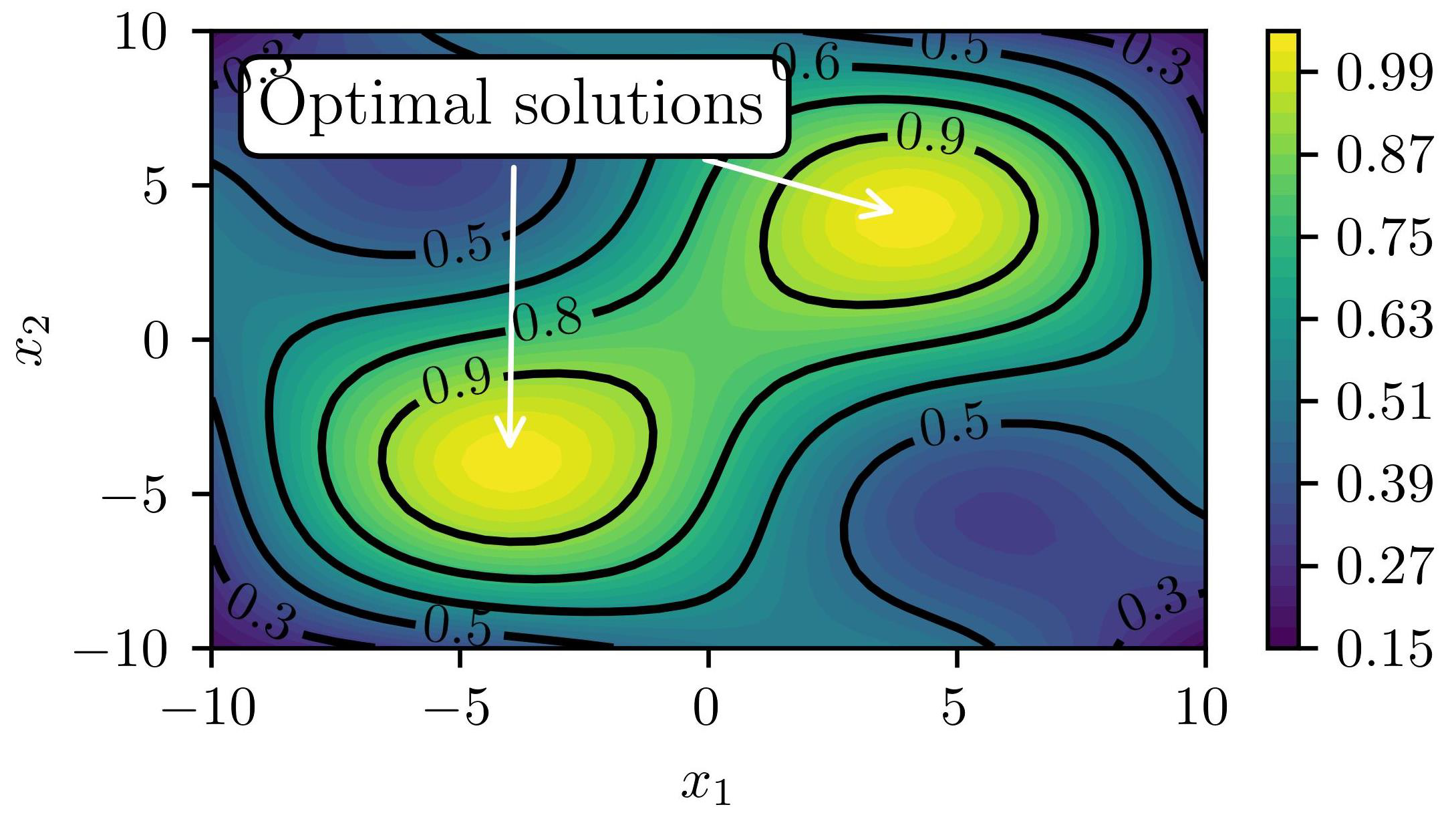
3.1. Objective and Outline

From the definition of A ( x ; β , θ ) , the search performance of GPBO depends on the KP θ . Due to the fact that the KP is obtained via GD, the maximum number of iterations for updating T g significantly affects the GPBO search performance. When the number of iterations T g is too high, the surrogate model is overfitted to the observation samples. In such cases, a relatively poor search performance is expected. When the exploration weight is set to a large value, because the observed samples occur in various regions in the input domain, the generalization error caused by overfitting may be mitigated. In contrast, when a small value is used for the exploration weight, because observation samples only occur in limited regions, the generalization error can be larger. Due to the fact that the generalization performance of the surrogate model affects the GPBO search performance, we consider that the negative effect of the overfitted KPs on the search performance depends on the exploration weight β . This hypothesis was verified through a simple numerical simulation.
We adopted the black-box function f ( x ) and its search space Ψ as follows:
f ( x ) = 1 3 sin x 1 3 sin x 2 3 ( x 1 ) 2 300 ( x 2 ) 2 300 + 5 6 , x Ψ : = [ 10 , 10 ] × [ 10 , 10 ] .
For simplicity, we set the observation noise to ϵ = 0 . The black-box function is shown in Figure 1. The adopted black-box function had two optimal solutions.
We used GPBO based on Algorithm 1, and the values of the input parameters are presented in Table 1. To verify the aforementioned hypothesis, the effects of the degree of kernel-parameter tuning and the exploration weight on the GPBO search performance were analyzed. Therefore, we adopted multiple values for the maximum number of GD iterations T g and exploration weight β . Moreover, the initial observation dataset D comprised four randomly selected points x 1 , , x 4 from the search space Ψ . To enhance the reliability of the results, we performed 20 experiments in which the same parameter conditions were used but the random seed identification was changed.

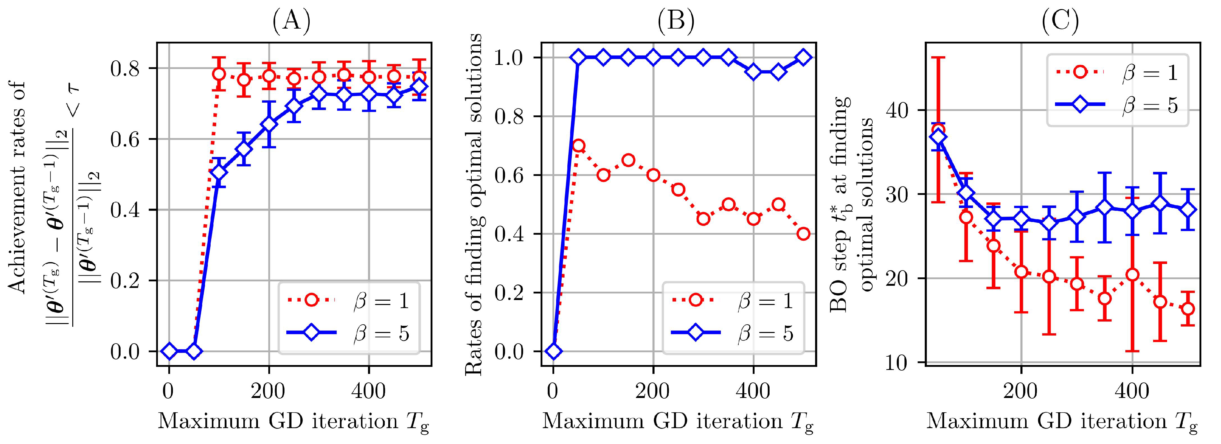
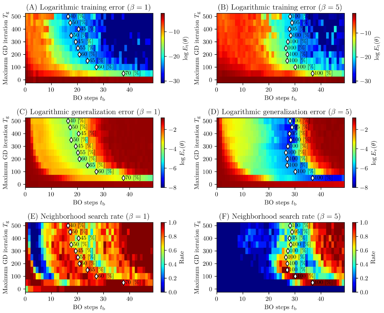
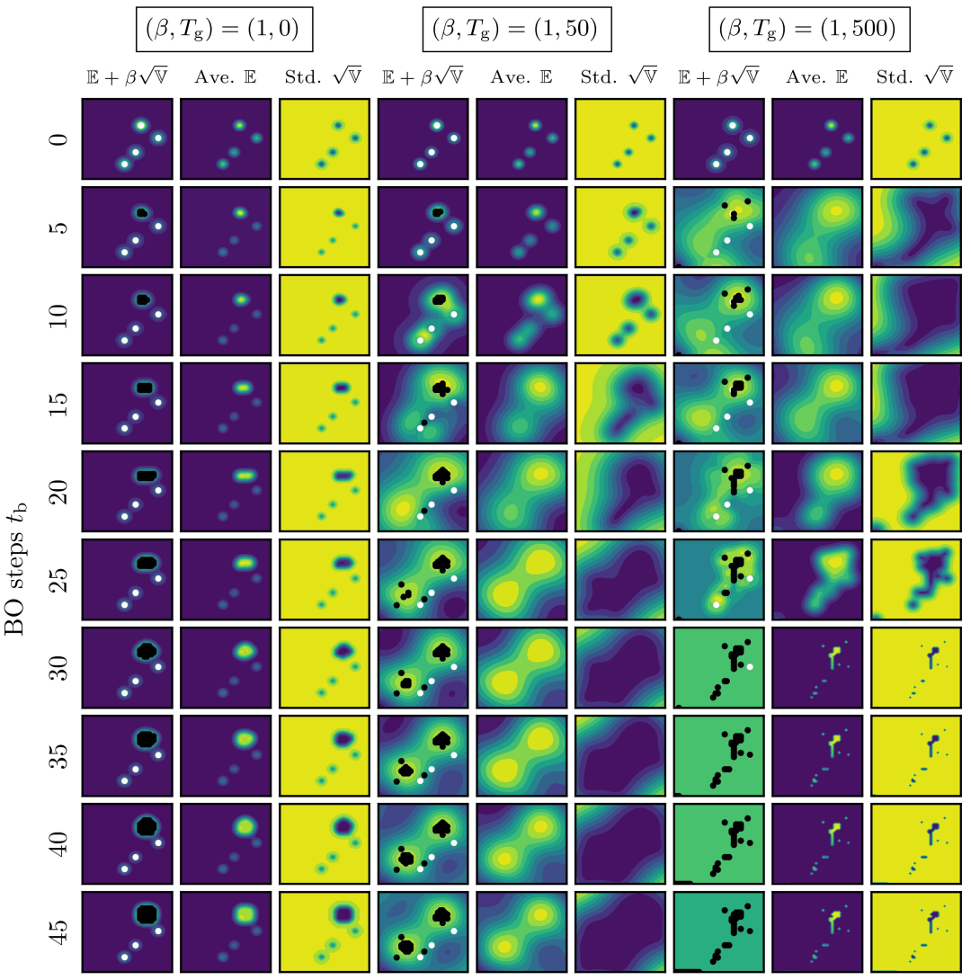
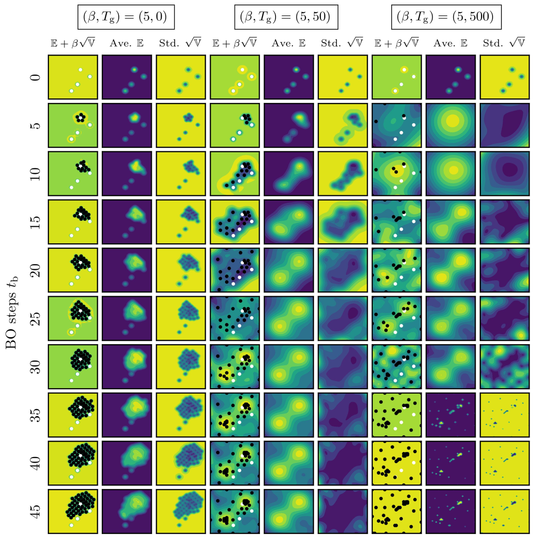
3.2. Results and discussions

The relationship between the maximum number of GD iterations and the kernel-parameter tuning is presented in Figure 2A. The figure shows the rate at which the KPs θ ( T g ) obtained via the GD of each Bayesian optimization step of 50 iterations converged. We investigated whether the convergence was determined by Equation (24) for τ = 0.01 . The results represent the averages of 20 trials with different seeds. For β = 1 and 5, Figure 2A suggests that the log-likelihood converged when the maximum number of GD iterations T g was set as more than approximately 300. Therefore, we regarded the KPs as overtuned at >300 GD iterations.
Figure 2B shows the rate of finding the two optimal solutions in 20 trials with different seeds. The maximum number of GD iterations was the degree of kernel-parameter tuning via GD. For β = 1 , a larger maximum number of GD iterations corresponded to worse search performance. In contrast, for β = 5 , even when the maximum number of GD iterations was large, the rates of finding solutions remained high. Therefore, we consider that even if KPs are overtuned to the observation dataset, in cases of a large exploration weight, GPBO can adequately search for solutions (of course, it is desirable to avoid overfitting). Figure 2C presents the average number of Bayesian optimization steps needed for finding two optimal solutions calculated using only the results where two optimal solutions were successfully found. As shown, for a smaller value of β and a larger number of KPs tuned, the optimal solutions were found faster. However, as shown in Figure 2B, the rate of correctly finding the optimal solutions was lower. Therefore, for a small β , the KPs should not be excessively tuned. In contrast, for a large β , the negative effect caused by the overtuned KPs was not observed.
Next, we verified the training error E t ( θ ) and generalization error E v ( θ ) defined by Equations (21) and (22) for analyzing the effect of the exploration weight β on the GPBO search performance. Figure 3A,B show the training errors. Figure 3C,D show the generalization errors. We transformed them into log errors, that is, using log E t ( θ ) instead of E t ( θ ) . As the maximum number of GD iterations T g and number of Bayesian optimization steps t b increased, the training errors decreased. In contrast, in the latter half of the Bayesian optimization process, a higher number of tuned KPs (i.e., larger T g ) corresponded to larger generalization errors. When the generalization error of the surrogate model was large, because the reliability of the first term of the acquisition function defined by Equation (16) was low, the GPBO search performance was poor. From these results, for β = 1 , we attribute the degradation of the GPBO search performance to the overtuning of the KPs, which increased the generalization error. For β = 5 , even when the KPs were overtuned, there were many regions with small generalization errors. Therefore, in this case, we consider that the GPBO search performance was not degraded.
When observation samples occur in a limited region, the generalization error is large, because the surrogate model based on these data cannot correctly estimate the output values of various regions in the search space. To verify this hypothesis, we used Equation (23) with ω = 0.5 and calculated the rate at which the next search point determined by Equation (17) and the observed points were close. The results are presented in Figure 3E,F. Figure 3E suggests that, when the exploration weight was set as β = 1 , the GPBO searched for areas close to previously observed samples. This was particularly true when large numbers of KPs were tuned. For example, in the case of β = 1 and T g = 500 , when the number of Bayesian optimization steps exceeded approximately 35 ( t b > 35 ), the search area of GPBO remained close to the previously observed samples. This trend was weaker for a smaller value of T g . Thus, there was a stronger tendency to search close to the previously observed samples when the KPs were overtuned. Therefore, we considered the GPBO search performance to be poor. Figure 3F suggests that, for β = 5 , the GPBO searched various areas even if the KPs were overtuned. In summary, from Figure 3E,F, the degree of kernel-parameter tuning affected whether GPBO searched areas close to previously observed samples. Moreover, a smaller exploration weight β corresponded to a higher risk. Thus, for a smaller value of β , there should be more focus on kernel-parameter tuning.
Next, we present the changes in the surrogate model for each Bayesian optimization step in Figure 4 and Figure 5. These values were β = 1 , 5 , respectively. Due to the fact that we cannot show the results for all the seeds, the results for a specific seed are shown. In the case where no KPs were tuned, that is, T g = 0 , appropriate searches were not performed regardless of β . For T g = 0 , Figure 3A–D indicate that the training and generalization errors were large. We believe that, because the surrogate model was inappropriate, the GPBO search was inappropriate.
With a small number of KPs tuned, i.e., T g = 50 , the average E generated from the surrogate model nearly succeeded in reproducing the black-box function f ( x ) regardless of β . Therefore, the rate of correctly finding the optimal solution was high (see Figure 2B).
Figure 4 and Figure 5 suggest that, when the number of iterations of KP tuning was T g = 500 , the search results depended on the exploration weight β . For β = 1 , because the GPBO searched only the neighborhood of the best point from the initial solutions, even if the search progressed, the output from the surrogate model E could not reproduce the black-box function f ( x ) . In contrast, for β = 5 , because observation samples appeared in various areas, even if the KPs were overtuned, the output of the surrogate model E reproduced the black-box function f ( x ) . The results indicate that the negative effect of overtuning the KPs on the GPBO search performance can be mitigated by increasing the exploration weight β .
However, in both the β = 1 and 5 cases, when the number of iterations of KP tuning increased ( T g = 500 ), the surrogate model output was inappropriate when the number of BO steps t b was approximately 30–35 (the cases of T g = 500 are shown in Figure 4 and Figure 5). In general, overfitting parameters to observed data increases the risk of reduced estimation performance in areas where there are no observed data. Therefore, overfitting can easily occur with high T g values. Due to the fact that this occurs in both the cases of β = 1 and 5, it is important not to overtune the KPs, regardless of the exploration weight. Although the negative effects of overtuned KPs can be mitigated by increasing the exploration weight, they cannot be completely eliminated.

4. Conclusions

The exploration weight affects the degree of exploration of GPBO. Therefore, the GPBO search performance depends on the exploration weight. In this study, we analyzed the mitigation of the negative effect of overtuning KPs as another effect of the exploration weight. The results indicate that we should pay attention to overtuning the KPs in the case of Bayesian optimization with a small exploration weight. It is preferable to use methods for avoiding the overtuning of KPs, e.g., early stopping of the GD. In contrast, for large exploration weights, the solution discovery rate is high even when overtuning the KPs. These findings are useful in all situations wherein GPBO is used, e.g., hyperparameter tuning in machine learning.
The results and discussions presented in this paper are entirely based on the black-box function defined by Equation (25). The function has two optimal solutions clearly visible in the domain. However, it is not known whether the results of this study would be reproduced if flat functions such as the Beale function [33] or the Goldstein–Price function [34] (the minimum search) were adopted. As shown in Figure 6, the structure of these functions is apparent after log transformation. A similar result can be obtained with a flat function, or a logarithmic transformation may have to be performed. These points are unclear and will be discussed in a future work.

Funding

This work was supported in part by JSPS Grants-in-Aid for Scientific Research (C) (Grant Nos. 21K04535 and 23K11310) and a JSPS Grant-in-Aid for Young Scientists (Grant No. 19K20062).

Institutional Review Board Statement

Not applicable.

Data Availability Statement

Not applicable.

Conflicts of Interest

The authors declare no conflict of interest.

References

  1. Saleh, E.; Tarawneh, A.; Naser, M.Z.; Abedi, M.; Almasabha, G. You only design once (YODO): Gaussian Process-Batch Bayesian optimization framework for mixture design of ultra high performance concrete. Constr. Build. Mater. 2022, 330, 127270. [Google Scholar] [CrossRef]
  2. Mathern, A.; Steinholtz, O.S.; Sjöberg, A.; Önnheim, M.; Ek, K.; Rempling, R.; Gustavsson, E.; Jirstrand, M. Multi-objective constrained Bayesian optimization for structural design. Struct. Multidiscip. Optim. 2021, 63, 689–701. [Google Scholar] [CrossRef]
  3. Frazier, P.I.; Wang, J. Bayesian optimization for materials design. Springer Ser. Mater. Sci. 2015, 225, 45–75. [Google Scholar] [CrossRef] [Green Version]
  4. Ohno, H. Empirical studies of Gaussian process based Bayesian optimization using evolutionary computation for materials informatics. Expert Syst. Appl. 2018, 96, 25–48. [Google Scholar] [CrossRef]
  5. Ueno, T.; Rhone, T.D.; Hou, Z.; Mizoguchi, T.; Tsuda, K. COMBO: An efficient Bayesian optimization library for materials science. Mater. Discov. 2016, 4, 18–21. [Google Scholar] [CrossRef] [Green Version]
  6. Elsayad, A.M.; Nassef, A.M.; Al-Dhaifallah, M. Bayesian optimization of multiclass SVM for efficient diagnosis of erythemato-squamous diseases. Biomed. Signal Process. Control 2022, 71, 103223. [Google Scholar] [CrossRef]
  7. Agrawal, A.K.; Chakraborty, G. On the use of acquisition function-based Bayesian optimization method to efficiently tune SVM hyperparameters for structural damage detection. Struct. Control. Health Monit. 2021, 28, e2693. [Google Scholar] [CrossRef]
  8. Xie, W.; Nie, W.; Saffari, P.; Robledo, L.F.; Descote, P.Y.; Jian, W. Landslide hazard assessment based on Bayesian optimization–support vector machine in Nanping City, China. Nat. Hazards 2021, 109, 931–948. [Google Scholar] [CrossRef]
  9. Wu, J.; Chen, X.Y.; Zhang, H.; Xiong, L.D.; Lei, H.; Deng, S.H. Hyperparameter Optimization for Machine Learning Models Based on Bayesian Optimization. J. Electron. Sci. Technol. 2019, 17, 26–40. [Google Scholar] [CrossRef]
  10. Kumar, P.; Nair, G.G. An efficient classification framework for breast cancer using hyper parameter tuned Random Decision Forest Classifier and Bayesian Optimization. Biomed. Signal Process. Control 2021, 68, 102682. [Google Scholar] [CrossRef]
  11. Snoek, J.; Larochelle, H.; Adams, R.P. Practical Bayesian Optimization of Machine Learning Algorithms. In Proceedings of the 25th International Conference on Neural Information Processing Systems, Lake Tahoe, NV, USA, 3–6 December 2012. [Google Scholar]
  12. Kolar, D.; Lisjak, D.; Pajak, M.; Gudlin, M. Intelligent Fault Diagnosis of Rotary Machinery by Convolutional Neural Network with Automatic Hyper-Parameters Tuning Using Bayesian Optimization. Sensors 2021, 21, 2411. [Google Scholar] [CrossRef] [PubMed]
  13. Snelson, E.; Ghahramani, Z. Local and global sparse Gaussian process approximations. In Proceedings of the Eleventh International Conference on Artificial Intelligence and Statistics, San Juan, Puerto Rico, 21–24 March 2007; pp. 524–531. [Google Scholar]
  14. Snelson, E.; Ghahramani, Z. Sparse Gaussian Processes using Pseudo-inputs. In Proceedings of the 18th International Conference on Neural Information Processing Systems, Vancouver, BC, Canada 5–8 December 2005. [Google Scholar]
  15. Csató, L.; Opper, M. Sparse On-Line Gaussian Processes. Neural Comput. 2002, 14, 641–668. [Google Scholar] [CrossRef] [PubMed] [Green Version]
  16. Seeger, M.W.; Williams, C.K.I.; Lawrence, N.D. Fast Forward Selection to Speed Up Sparse Gaussian Process Regression. In Proceedings of the Ninth International Workshop on Artificial Intelligence and Statistics, Key West, FL, USA, 3–6 January 2003; pp. 254–261. [Google Scholar]
  17. Chen, H.; Zheng, L.; Kontar, R.A.; Raskutti, G. Gaussian Process Parameter Estimation Using Mini-batch Stochastic Gradient Descent: Convergence Guarantees and Empirical Benefits. J. Mach. Learn. Res. 2022, 23, 1–59. [Google Scholar]
  18. Martino, L.; Laparra, V.; Camps-Valls, G. Probabilistic cross-validation estimators for Gaussian Process regression. In Proceedings of the 25th European Signal Processing Conference, EUSIPCO 2017, Kos, Greece, 28 August–2 September 2017; pp. 823–827. [Google Scholar] [CrossRef]
  19. Zhang, R.; Zhao, X. Inverse Method of Centrifugal Pump Blade Based on Gaussian Process Regression. Math. Probl. Eng. 2020, 2020, 4605625. [Google Scholar] [CrossRef]
  20. Senanayake, R.; O’callaghan, S.; Ramos, F. Predicting Spatio-Temporal Propagation of Seasonal Influenza Using Variational Gaussian Process Regression. Proc. AAAI Conf. Artif. Intell. 2016, 30, 3901–3907. [Google Scholar] [CrossRef]
  21. Petelin, D.; Filipic, B.; Kocijan, J. Optimization of Gaussian process models with evolutionary algorithms. In Lecture Notes in Computer Science (Including Subseries Lecture Notes in Artificial Intelligence and Lecture Notes in Bioinformatics); Springer: Berlin/Heidelberg, Germany, 2011; Volume 6593, pp. 420–429. [Google Scholar] [CrossRef]
  22. Ouyang, Z.L.; Zou, Z.J. Nonparametric modeling of ship maneuvering motion based on Gaussian process regression optimized by genetic algorithm. Ocean Eng. 2021, 238, 109699. [Google Scholar] [CrossRef]
  23. Cheng, L.; Ramchandran, S.; Vatanen, T.; Lietzen, N.; Lahesmaa, R.; Vehtari, A.; Lähdesmäki, H. LonGP: An additive Gaussian process regression model for longitudinal study designs. bioRxiv 2018, 259564. [Google Scholar] [CrossRef] [Green Version]
  24. Israelsen, B.; Ahmed, N.; Center, K.; Green, R.; Bennett, W., Jr. Adaptive Simulation-Based Training of Artificial-Intelligence Decision Makers Using Bayesian Optimization. J. Aerosp. Comput. Inf. Commun. 2018, 15, 38–56. [Google Scholar] [CrossRef]
  25. Rasmussen, C.E.; Williams, C.K.I. Gaussian Processes for Machine Learning; MIT Press: Cambridge, MA, USA, 2006. [Google Scholar]
  26. Deringer, V.L.; Bartók, A.P.; Bernstein, N.; Wilkins, D.M.; Ceriotti, M.; Csányi, G. Gaussian Process Regression for Materials and Molecules. Chem. Rev. 2021, 121, 10073–10141. [Google Scholar] [CrossRef]
  27. Oliveira, R.; Ott, L.; Ramos, F. Bayesian optimisation under uncertain inputs. In Proceedings of the Twenty-Second International Conference on Artificial Intelligence and Statistics, Naha, Japan, 16–18 April 2019; Volume 89, pp. 1177–1184. [Google Scholar]
  28. Ath, G.D.; Everson, R.M.; Rahat, A.A.M.; Fieldsend, J.E. Greed is Good: Exploration and Exploitation Trade-offs in Bayesian Optimisation. ACM Trans. Evol. Learn. Optim. 2021, 1, 1–22. [Google Scholar] [CrossRef]
  29. Mochihashi, D.; Oba, S. Gaussian Process and Machine Learning; Kodansha Scientific: Tokyo, Japan, 2019. [Google Scholar]
  30. Blonigen, B.A.; Knittel, C.R.; Soderbery, A. Keeping it Fresh: Strategic Product Redesigns and Welfare. Int. J. Ind. Organ. 2017, 53, 170–214. [Google Scholar] [CrossRef] [Green Version]
  31. Mareček, R.; Řĺha, P.; Bartoňová, M.; Kojan, M.; Lamoš, M.; Gajdoš, M.; Vojtĺšek, L.; Mikl, M.; Bartoň, M.; Doležalová, I.; et al. Automated fusion of multimodal imaging data for identifying epileptogenic lesions in patients with inconclusive magnetic resonance imaging. Hum. Brain Mapp. 2021, 42, 2921–2930. [Google Scholar] [CrossRef] [PubMed]
  32. Che, K.; Chen, X.; Guo, M.; Wang, C.; Liu, X. Genetic Variants Detection Based on Weighted Sparse Group Lasso. Front. Genet. 2020, 11, 155. [Google Scholar] [CrossRef] [PubMed]
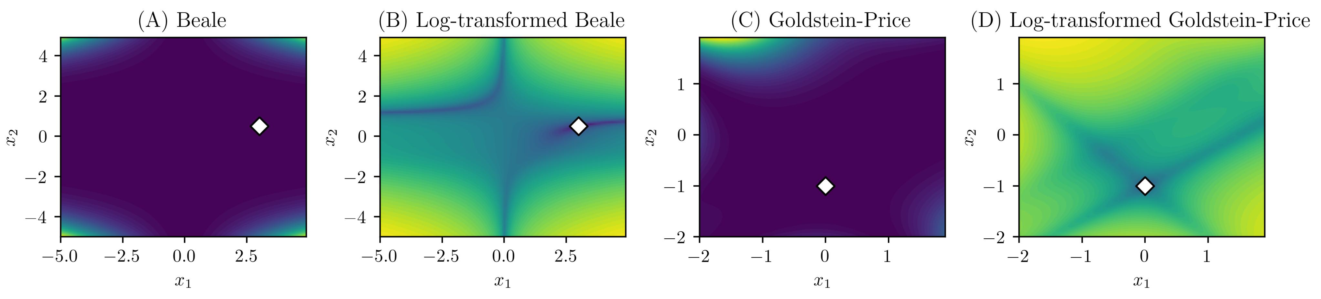
  33. Surjanovic, S.; Bingham, D. Beale Function. 2013. Available online: https://www.sfu.ca/~ssurjano/beale.html (accessed on 27 June 2023).
  34. Surjanovic, S.; Bingham, D. Goldstein-Price Function. 2013. Available online: https://www.sfu.ca/~ssurjano/goldpr.html (accessed on 27 June 2023).
Figure 1. Adopted black-box function f ( x ) defined by Equation (25).
Mathematics 11 03067 g001
Figure 2. Relationships between the maximum number of GD iterations and other indices. Figure (A) presents the convergence achievement rates for Equation (24). (First, we averaged the results of all the Bayesian optimization steps ( T b = 50 ). Then, the averages and standard deviations of the results for 20 seeds were calculated.) Figure (B) presents the rates of finding two optimal solutions (total of 20 seeds). Figure (C) presents the average number of optimization steps needed for finding two optimal solutions calculated with only the results where two optimal solutions were successfully found (total of 20 seeds). The error bars indicate the standard deviations.
Mathematics 11 03067 g002
Figure 3. (A,B) Training errors of surrogate models calculated using Equation (21) for each maximum number of GD iterations; (C,D) generalization errors calculated using Equation (22); (E,F) rates of exploring the neighborhood of past observed samples. The values of (AD) are the averages of 20 seeds, and those of (E,F) are the rates of 20 seeds. The white markers indicate the timings of finding two optimal solutions, and the percentages are the success rates of finding them in 20 trials with different seeds. These results are presented in Figure 2B,C. In the cases of β = 1 , with a larger maximum number of GD iterations, although a solution was found faster, the success rate was worse. At β = 5 , no such trend was observed.
Mathematics 11 03067 g003
Figure 4. Average E , standard deviation V of the surrogate model, and the acquisition function E + β V for the maximum number of GD iterations T g and exploration weight β = 1 calculated using Equations (3), (4) and (16). The white circles represent initial points, and the black circles represent observation points selected by the acquisition function.
Mathematics 11 03067 g004
Figure 5. Average E , standard deviation V of the surrogate model, and the acquisition function E + β V for the maximum number of GD iterations T g and exploration weight β = 5 calculated using Equations (3), (4) and (16). The white circles represent initial points, and the black circles represent observation points selected by the acquisition function.
Mathematics 11 03067 g005
Figure 6. (A) Beale function [33], (B) log-transformed Beale function, (C) Goldstein–Price function [34], and (D) log-transformed Goldstein–Price function. The white diamond mark represents the global optimal solution.
Mathematics 11 03067 g006
Table 1. Input values for Algorithm 1. { · } is a set consisting of multiple elements, i.e., multiple patterns were adopted.
ParametersValue(s)
Maximum number of GD iterations T g { 0 , 50 , 100 , , 500 }
GD learning rate γ 0.01
Maximum number of BO iterations T b 50
Exploration weight β { 1 , 5 }
Initial KP θ ( 0 ) [ 1 1 1 ]
Search space Ψ Equation (25)
Black-box function f ( x ) Equation (25)
Observation noise ϵ 0
Initial observation dataset D Four points randomly selected in Ψ
Disclaimer/Publisher’s Note: The statements, opinions and data contained in all publications are solely those of the individual author(s) and contributor(s) and not of MDPI and/or the editor(s). MDPI and/or the editor(s) disclaim responsibility for any injury to people or property resulting from any ideas, methods, instructions or products referred to in the content.

