Riemannian Formulation of Pontryagin’s Maximum Principle for the Optimal Control of Robotic Manipulators

Abstract

In this work, we consider robotic systems for which the mass tensor is identified to be the metric in a Riemannian manifold. Cost functional invariance is achieved by constructing it with the identified metric. Optimal control evolution is revealed in the form of a covariant second-order ordinary differential equation featuring the Riemann curvature tensor that constrains the control variable. In Pontryagin’s framework of the maximum principle, the cost functional has a direct impact on the system Hamiltonian. It is regarded as the performance index, and optimal control variables are affected by this fundamental choice. In the present context of cost functional invariance, we show that the adjoint variables are the first-order representation of the second-order control variable evolution equation. It is also shown that adding supplementary invariant terms to the cost functional does not modify the basic structure of the optimal control covariant evolution equation. Numerical trials show that the proposed invariant cost functionals, as compared to their non-invariant versions, lead to lower joint power consumption and narrower joint angular amplitudes during motion. With our formulation, the differential equations solver gains stability and operates dramatically faster when compared to examples where cost functional invariance is not considered.

1. Introduction

Three of the main preoccupations in robotics have for a long time been the modeling, the planning, and the control of robots. Indeed, motion planning is about finding a path for the modeled system, which satisfies the desired task. Subsequently, control enables the robot to follow the planned trajectory by guaranteeing its feasibility [1]. Thus, naturally, some of the most influential books in the field are dedicated to analyzing these matters [2,3,4,5].

Optimal control can be considered to be a bridge between planning and control in the sense that the planned motion does not purely obey geometrical considerations in the task space. Configuration parameters and their derivatives, as well as forces, are often taken into account [6,7]. This implies that restrictions on these parameters can also be taken into account during the planning stage, so that the controller focuses mainly on the stability and robustness of the trajectory tracking process. Among the optimal control methods, the application of Pontryagin’s maximum principle [8,9,10] is certainly one of the most broadly used (some robotics-related examples can be found in [11,12,13,14,15]). It provides an optimality condition that requires to be met at each time during the trajectory. The method generally involves restrictions in the form of ordinary differential equations (ODE), which are usually of the first order, therefore limiting the computational cost of their solution up to a certain extent (as implied in [10]).

One particular class of robots that has historically received much attention is that of robotic manipulators. These are typically used for industrial purposes, to perform repetitive “pick-and-place” tasks in order to increase production [16,17]. However, these have also been commonly used in more complex situations, serving for example as the upper limbs of some humanoid robots [18,19].

When deriving the equations of motion of robotic manipulators from a Lagrangian perspective, an underlying geometric structure is easily recognizable. Indeed, Christoffel symbols (of the first kind) arise and describe the effect of Coriolis and centrifugal forces on the robot links [3,5,16], even with classical model representations. Unsurprisingly, differential and Riemannian geometry have been previously used to model robotic systems [20,21,22,23,24]. These geometric formulations of robot motion dynamics have given important insights. For example, it has been previously identified that the robot mass tensor defines a Riemannian metric [20,21,24,25]. However, perhaps a rather interesting result is that when a manipulator mass tensor (the metric) has a vanishing Riemannian curvature, such as a balanced two degrees of freedom (DOF) manipulator, there exists a set of coordinates in which the motion equations become very simple [20]. The emergence of the Riemann curvature tensor in robot modeling is not common, and for this particular result, the author states that it should be more useful for manipulator analysis and design than for their direct control [20]. We shall see in this paper that the Riemann tensor naturally emerges in the context of the optimal control of robotic manipulators.

It is undeniable that geometry enables a certain understanding of physical phenomena. A remarkable analysis of the role that geometry plays in the process of motion generation (be it human or robotic) can be found in [26]. In our work, we propose a geometric formulation of Pontryagin’s maximum principle as applied to the optimal control problem of a robotic manipulator. We take up the idea that the robot mass tensor is the Riemannian metric and therefore construct an invariant running cost function where the policy is both torque and energy consumption minimization. Through variational principles first, and through Pontryagin’s maximum principle then, we propose an intrinsic covariant evolution of the optimal force required to produce motion. These equations that we call “covariant control equations” feature geometric objects, including the Riemann curvature tensor. The latter is enabled by our choice of an invariant cost function. Simulations of optimal motion show the benefits of our approach from a numerical perspective as well as from the resulting motion characteristics perspective. Our focus is on computing the forces required to cause optimal motion. Therefore, other applications of the maximum principle such as tracking problems or output feedback [27] are not discussed in the present work.

We begin by setting up our framework in Section 2 by introducing the chosen metric, the manifold tools, and the system modeling in a Riemannian formulation. Then, the background of our optimal control formulation is presented in Section 3, and we propose an invariant cost function for the optimal control of robotic manipulators in Section 4. A second-order covariant time evolution for the optimal forces required to cause motion is proposed with the corresponding proof. It is shown that a basic geometric structure is preserved with respect to previous developments. Then, Section 5 is devoted to giving a Riemannian formulation of Pontryagin’s maximum principle for the optimal control of robotic manipulators using our invariant cost functions. Physical interpretation for one of the adjoint variables results from the optimality condition. We also prove that the adjoint variables are fundamentally related and lead to our proposed covariant control equations. Finally, the impact of our Riemannian formulation of the maximum principle, on a general purpose ODE solver, is evaluated through numerical simulations of optimally controlled motion in Section 6. This last section presents the advantages on numerical robustness and on the resulting motion characteristics.

2. Riemannian Manifold

We regard robotic manipulators as multibody dynamical systems parameterized by a finite number n of configuration parameters $q^i$ where $i\in [1,n]$. Focus is set on the class of serial manipulators in which each joint supports another one further down the chain. Thus, each joint motion is ensured by an actuator placed between two neighboring segments, which exerts torque action. Q denotes the set of states $q\equiv \left\{q^i\right\}$. In the whole document, we will rely on tensor notation and apply Einstein’s summation convention on repeated indices [28,29].

2.1. Metric

Our framework relies on deriving robot dynamics from the system kinetic energy K, which is a quadratic and strictly convex form of ${\dot{q}}^i$, where the overdot denotes the rate of change with respect to time. The coefficients of K define a positive definite, configuration-dependent Hessian $M\left(q\right)$, called the mass tensor. Mass tensor components are formed by nonlinear regular functions of the state $q\in Q$. The system kinetic energy is expressed as

$$K(q,\dot{q})=\frac{1}{2}{M}_{kl}\left(q\right){\dot{q}}^k{\dot{q}}^l.$$

(1)

The mass tensor $M\left(q\right)$ is a measure of the mass distribution and inertia of the multibody system [30]. Being symmetric and positive definite, it constitutes a perfect candidate to define a metric g in a Riemannian manifold, and it has previously been identified to be one in the context of robot modeling [20,21,24,25]. Therefore, we set

$$g_{kl}\left(q\right)\equiv M_{kl}\left(q\right).$$

(2)

2.2. Manifold Tools

Therefore, the space of states Q has the structure of a Riemannian manifold in which the following tools of Riemannian geometry apply (see [28,29]).

(a)

Covariant space derivation ${\partial }_j\equiv q^j$.

(b)

Contravariant space derivation ${\partial }^k=M^{jk}{\partial }_j$.

(c)

Relationship between a vector basis $e^j$, and its dual $e_k$ such that $⟨e^j,e_k⟩={\delta }_k^j$.

(d)

Components of the inverse mass tensor $M^{-1}=M^{jl}$ such that $M_{ij}{M}^{jl}={\delta }_i^l$.

(e)

The connection ${\Gamma }_{ik}^l=\frac{1}{2}{M}^{jl}\left({\partial }_i{M}_{lk}+{\partial }_k{M}_{li}-{\partial }_l{M}_{ik}\right)$ is symmetric ${\Gamma }_{ki}^j={\Gamma }_{ik}^j$ and defines the differentials $\mathrm{d}{e}_j={\Gamma }_{jk}^l\mathrm{d}{q}^k{e}_l$ and $\mathrm{d}{e}^j=-{\Gamma }_{kl}^j\mathrm{d}{q}^k{e}^l$.

(f)

The relationship between covariant components ${\phi }_j$ and contravariant components ${\phi }^k$ is established through the metric: ${\phi }_j=M_{jk}{\phi }^k$, ${\phi }^k=M^{kj}{\phi }_j$.

(g)

Covariant differential of a vector field $\phi \equiv {\phi }^j{e}_j$: $\mathrm{d}\phi =\left({\partial }_l{\phi }^j+{\Gamma }_{lk}^j{\phi }^k\right)\mathrm{d}{q}^l{e}_j$.

(h)

Covariant differential of a covector field $\phi \equiv {\phi }_l{e}^l$: $\mathrm{d}\phi =\left({\partial }_k{\phi }_l-{\Gamma }_{kl}^j{\phi }_j\right)\mathrm{d}{q}^k{e}^l$.

(i)

Ricci’s identities

$$\left\{\begin{array}{ccc}\hfill {\partial }_j{M}_{kl}& =& {\Gamma }_{jk}^p{M}_{lp}+{\Gamma }_{jl}^p{M}_{kp}\hfill \\ \hfill {\partial }_j{M}^{kl}& =& -{\Gamma }_{jp}^k{M}^{pl}-{\Gamma }_{jp}^l{M}^{pk}.\hfill \end{array}\right.$$

(3)

(j)

Covariant derivative of a scalar field: $\mathrm{d}V={\partial }_{l}V\mathrm{d}{q}^l=⟨\nabla V,\mathrm{d}{q}^j{e}_j⟩$ and $\nabla V={\partial }_{l}V{e}^l$.

(k)

Covariant derivative of a covector field $\phi ={\phi }_l{e}^l$: $\mathrm{d}\phi \equiv ⟨\nabla \phi ,\mathrm{d}{q}^j{e}_j⟩$ and $\nabla \phi =\left({\partial }_k{\phi }_l-{\Gamma }_{kl}^j{\phi }_j\right)e^k{e}^l$.

(l)

Second covariant derivative of a scalar field V: ${\nabla }^{2}V=\nabla (\nabla V)$ becomes

$${\nabla }^{2}V=\left({\partial }_k{\partial }_{l}V-{\Gamma }_{kl}^j{\partial }_{j}V\right)e^k{e}^l.$$

(4)

(m)

Components $R_{ikl}^j$ of the Riemann curvature tensor:

$$R_{ikl}^j={\partial }_l{\Gamma }_{ik}^j-{\partial }_k{\Gamma }_{il}^j+{\Gamma }_{ik}^p{\Gamma }_{pl}^j-{\Gamma }_{il}^p{\Gamma }_{pk}^j.$$

(5)

(n)

Anti-symmetry of the Riemann curvature tensor: $R_{ikl}^j=R_{ilk}^j$.

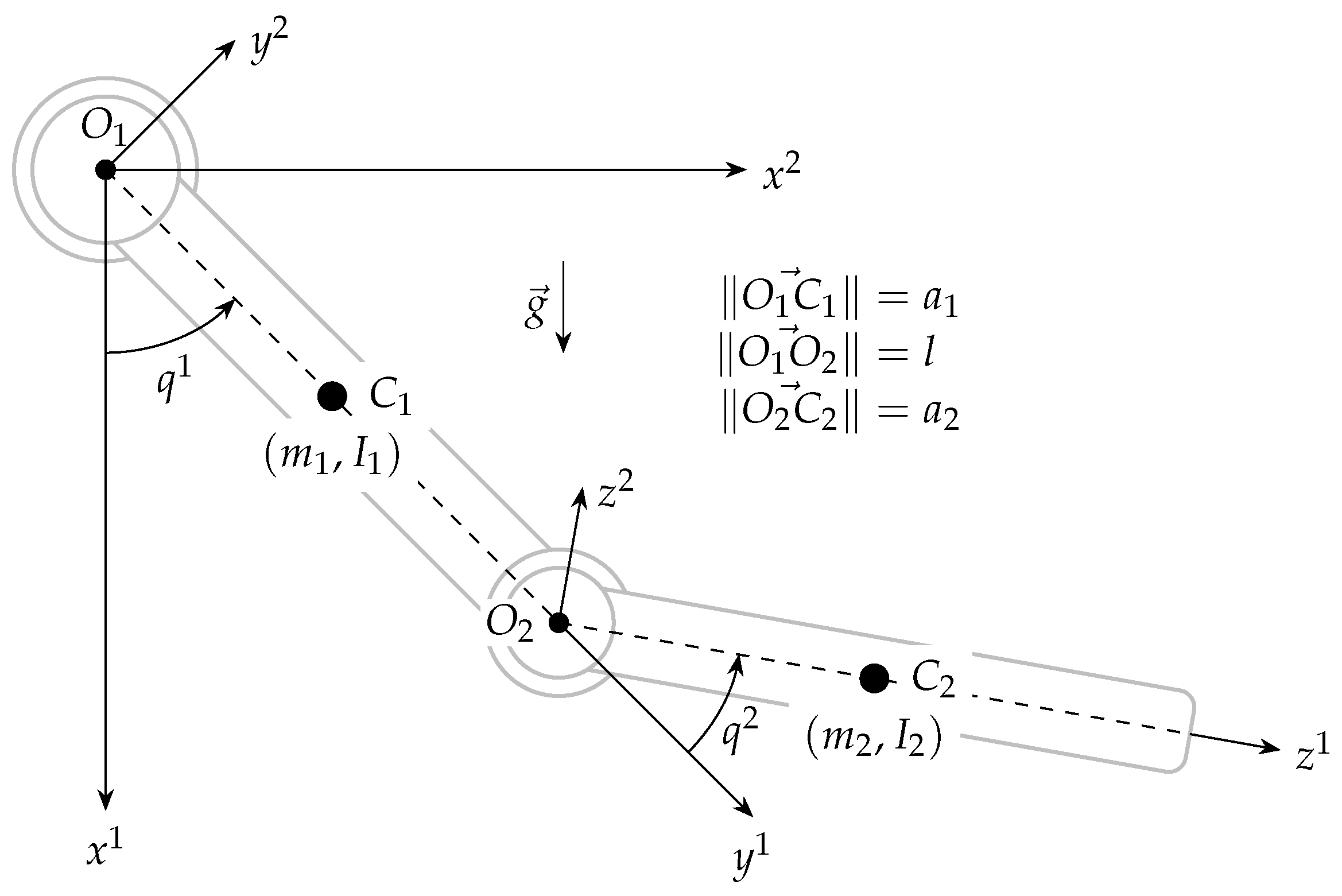
2.3. Manipulator Dynamics

Along with the kinetic energy defined by (1), we consider the gravitational potential $V=V\left(q\right)$, which is configuration dependent. This potential models gravity actions and is defined as a product between the system mass, the local gravitational field intensity, and the center of mass height.

The system Lagrangian is defined as $L(q,\dot{q})=K(q,\dot{q})-V\left(q\right)$. When a forcing control $u_i$ is exerted at the joint (typically a torque for our class of robots), the Euler–Lagrange equations that describe the dynamics for each of the generalized coordinates

$$\frac{\mathrm{d}}{\mathrm{d}t}\left(\frac{\partial L}{\partial {\dot{q}}^i}\right)-\frac{\partial L}{\partial q^i}=u_i$$

(6)

must be satisfied (see [24,30]). Upon inserting (1), the covariant second-order equations of motion are found [24,31,32]:

$$M_{kl}\left({\ddot{q}}^l+{\Gamma }_{ij}^l{\dot{q}}^i{\dot{q}}^j\right)+{\partial }_{k}V=u_k.$$

(7)

Thus, the robotic manipulator motion is governed by Equation (7). By recalling that $u^j=M^{ji}{u}_i$, the contravariant components of the torques u can be formulated:

$${\ddot{q}}^j+{\Gamma }_{kl}^j{\dot{q}}^k{\dot{q}}^l+M^{jl}{\partial }_{l}V=u^j.$$

(8)

Note that Equations (7) and (8) can be presented in a more compact form. This is achieved by noticing that the first two terms of the above equations compose the second covariant time derivative of the configuration parameter q. Recall that

$$\frac{\mathrm{d}q}{\mathrm{d}t}={\dot{q}}^i{e}_i.$$

(9)

This expression can be differentiated again by considering property (e) of Section 2.2:

$$\frac{{\mathrm{d}}^{2}q}{\mathrm{d}{t}^2}=\frac{\mathrm{d}}{\mathrm{d}t}\left({\dot{q}}^i{e}_i\right)={\ddot{q}}^i{e}_i+{\dot{q}}^i\frac{\mathrm{d}{e}_i}{\mathrm{d}t}=\left({\ddot{q}}^i+{\Gamma }_{jk}^i{\dot{q}}^j{\dot{q}}^k\right)e_i.$$

(10)

Therefore, the covariant components (7) of the generalized force take the compact form

$$M_{kl}{\left(\frac{{\mathrm{d}}^{2}q}{\mathrm{d}{t}^2}\right)}^l+{\partial }_{k}V=u_k,$$

(11)

and the contravariant components (8) become

$${\left(\frac{{\mathrm{d}}^{2}q}{\mathrm{d}{t}^2}\right)}^j+{\partial }^{j}V=u^j.$$

(12)

Finally, the system dynamics can be established as a first-order system by introducing a variable $\zeta$, so that, according to (8),

$$\left\{\begin{array}{ccc}\hfill {\dot{q}}^j-{\zeta }^j& =& 0\hfill \\ \hfill {\dot{\zeta }}^j+{\Gamma }_{kl}^j{\zeta }^k{\zeta }^l& =& u^j-M^{jl}{\partial }_{l}V.\hfill \end{array}\right.$$

(13)

3. Riemannian Formulation of Optimal Control Background

Our optimal control problem can be summarized as the following: we wish to take the robotic system from an initial state to a final state in a prescribed time T such that the control action minimizes a chosen performance index. We select the performance index (as called in [7]) or cost functional (as called in [10]) to be an integral of the type

$${\displaystyle J\left(u\right)=\underset{0}{\overset{T}{\int }}\gamma \left(u(q,\dot{q},\ddot{q})\right)\mathrm{d}t,}$$

(14)

where u denotes the control variable. Let U denote the set of controls $u\equiv \left\{u^i\right\}$, which are assumed to belong to a restricted class of smooth, sufficiently differentiable functions in the domain $[0,T]$. It is deemed admissible if it satisfies the imposed boundary conditions [9]. Such control action can be constrained by minimizing (14) either by applying traditional variational techniques or by applying Pontryagin’s maximum principle [8,10]. The function $\gamma =\gamma \left(u\right)$ is control dependent and defines the running cost [10]. It is assumed to be continuously differentiable in $t\in \mathbb{R}$, $q\in Q$ and $u\in U$. In our work, we will refer to $J\left(u\right)$ as the performance index and to $\gamma$ as the running cost function. We will refrain from addressing to $J\left(u\right)$ as cost functional in order to avoid confusion with the running cost function $\gamma$.

The running cost function $\gamma$ can be selected to be convex in order to ease the minimization of (14). Additionally, in order to preserve a Riemannian structure, $\gamma$ should be chosen to be invariant and preferably composed by the metric $M\left(q\right)$. By choosing the particular running cost function ${\gamma }_1=u_i{u}^i$, the performance index is

$${\displaystyle J\left(u\right)=\underset{0}{\overset{T}{\int }}{\gamma }_1\left(u\right)\mathrm{d}t=\underset{0}{\overset{T}{\int }}\frac{1}{2}{M}_{kl}\left(q\right)u^k{u}^l\mathrm{d}t.}$$

(15)

It has been shown [31,32] that the optimal control variable evolves according to the following second-order nonlinear ODE:

$${\left(\frac{{\mathrm{d}}^{2}u}{\mathrm{d}{t}^2}\right)}_j+R_{klj}^i{\dot{q}}^k{\dot{q}}^l{u}_i+\left({\nabla }_{jk}^{2}V\right)u^k=0,$$

(16)

where from [32] (Equation (17)),

$${\left(\frac{{\mathrm{d}}^{2}u}{\mathrm{d}{t}^2}\right)}_i={\ddot{u}}_i-{\Gamma }_{ij}^k\left(u_k{\ddot{q}}^j+2{\dot{u}}_k{\dot{q}}^j\right)-\left({\partial }_l{\Gamma }_{ij}^k-{\Gamma }_{ji}^m{\Gamma }_{ml}^k\right){\dot{q}}^j{\dot{q}}^l{u}_k.$$

(17)

Equation (16) is a result that was first established in the framework of the classical calculus of variations in [33]; it was later established in the framework of Pontryagin’s maximum principle in [31], further proving the equivalence of both techniques; and it was recently experimentally applied to the optimal control of a robotic manipulator in [32] through the framework of the classical calculus of variations. We shall refer to (16) as the “covariant control equations”, where we shall notice the explicit presence of the Riemann curvature tensor. The emergence of this quantity, although uncommon in robot modeling and control, confirms that since we have the metric and the connection (see properties (e) and (f) in Section 2.2), the curvature is never far away. This curvature can be interpreted as a robot dynamic response sensitivity measure to certain inertial parameters [20].

Therefore, when the selected running cost function is ${\gamma }_1$, the optimal control problem becomes that of solving a coupled system of nonlinear second-order ODE involving the manipulator equations of motion (11) and the covariant control Equation (16):

$$\left\{\begin{array}{ccc}\hfill {\displaystyle {\left(\frac{{\mathrm{d}}^{2}u}{\mathrm{d}{t}^2}\right)}_j+{\partial }_{j}V}& =& u_j\hfill \\ \hfill {\displaystyle {\left(\frac{{\mathrm{d}}^{2}u}{\mathrm{d}{t}^2}\right)}_j+\left({\nabla }_{jk}^{2}V\right)u^k}& =& R_{kjl}^i{\dot{q}}^k{\dot{q}}^l{u}_i,\hfill \end{array}\right.$$

(18)

with selected initial and final conditions on q and $\dot{q}$. The system (18) is contravariant in the states q and covariant in the control variable u. This set of equations can be solved with an appropriate ODE solver, Runge–Kutta-based integrators [34], or Finite Element-based methods such as the one presented in [35].

4. Optimal Dynamics with a Velocity Cost

We wish to further generalize the previous result of Equation (16). In particular, we are interested in adding a velocity cost to the performance index (15) in order to diminish motion amplitude. We will show in the present section that adding an invariant function of the generalized velocities does not modify the basic structure of Equation (16).

4.1. Generalization of Covariant Control Equations Structure

Let us consider the following performance index.

$$J\left(u\right)={\int }_0^T\frac{1}{2}\left[u_i{u}^i+\alpha {\dot{q}}_i{\dot{q}}^i\right]\mathrm{d}t,$$

(19)

where $\alpha$ is a scalar that ensures homogeneity. Let us call its integrand ${\gamma }_2$, which is the running cost function. By property (f) of Section 2.2,

$${\gamma }_2=\frac{1}{2}\left[M_{ij}\left(q\right)u^i{u}^j+\alpha M_{ij}\left(q\right){\dot{q}}^i{\dot{q}}^j\right].$$

(20)

The first term is an invariant convex function of the control variable u. The second term is an invariant convex function of the generalized velocities $\dot{q}$, which corresponds to the system kinetic energy, scaled by $\alpha$.

Proposition 1.

Covariant control equations: optimal force evolution.

With the above performance index (19), the optimal generalized forces u satisfy the following time evolution:

$${\left(\frac{{\mathrm{d}}^{2}u}{\mathrm{d}{t}^2}\right)}_i+\left({\nabla }_{il}^{2}V\right)u^l=R_{jli}^k{\dot{q}}^j{\dot{q}}^l{u}_k+\alpha {\left(\frac{{\mathrm{d}}^{2}q}{\mathrm{d}{t}^2}\right)}_j.$$

(21)

Proof of Proposition 1. 

According to (7) and (8), $u=u(q,\dot{q},\ddot{q})$. Therefore, we can apply the so-called Euler–Lagrange equations to the proposed performance index (19) as:

$$\frac{{\mathrm{d}}^2}{\mathrm{d}{t}^2}\left(\frac{\partial {\gamma }_2}{\partial {\ddot{q}}^i}\right)-\frac{\mathrm{d}}{\mathrm{d}t}\left(\frac{\partial {\gamma }_2}{\partial {\dot{q}}^i}\right)+\frac{\partial {\gamma }_2}{\partial q^i}=0.$$

(22)

Then, we have that

$$\left\{\begin{array}{ccc}\hfill {\displaystyle \frac{\partial {\gamma }_2}{\partial {\ddot{q}}^i}}& =& {\displaystyle \frac{1}{2}{M}_{jk}\frac{d}{d{\ddot{q}}^i}\left(u^j{u}^k\right)=M_{jk}\frac{d{u}^j}{d{\ddot{q}}^i}{u}^k=M_{jk}{u}^k=u_j}\hfill \\ \hfill {\displaystyle \frac{\partial {\gamma }_2}{\partial {\dot{q}}^i}}& =& 2{\Gamma }_{ij}^k{\dot{q}}^j{u}_k+\alpha M_{ij}{\dot{q}}^j\hfill \\ \hfill {\displaystyle \frac{\partial {\gamma }_2}{\partial q^i}}& =& {\displaystyle \frac{1}{2}\left({\partial }_i{M}^{jk}\right)u_j{u}_k+u^j{\partial }_i{u}_j+\frac{\alpha }{2}\left({\partial }_i{M}_{jk}\right){\dot{q}}^j{\dot{q}}^k,}\hfill \end{array}\right.$$

(23)

where from (7),

$$\begin{array}{cc}\hfill u^j{\partial }_i{u}_j& =u^j\left[\left({\partial }_i{M}_{jk}\right){\ddot{q}}^k+\left({\partial }_i{M}_{jm}\right){\Gamma }_{kl}^m{\dot{q}}^k{\dot{q}}^l+M_{jm}\left({\partial }_i{\Gamma }_{kl}^m\right){\dot{q}}^k{\dot{q}}^l+\left({\partial }_i{\partial }_{j}V\right)\right]\hfill \\ \hfill & =u^j\left[{\partial }_i{M}_{jk}({\ddot{q}}^k+{\Gamma }_{jl}^k{\dot{q}}^j{\dot{q}}^l)+M_{jm}\left({\partial }_i{\Gamma }_{kl}^m\right){\dot{q}}^k{\dot{q}}^l+\left({\partial }_i{\partial }_{j}V\right)\right]\hfill \\ \hfill & =u^j\left[{\partial }_i{M}_{jk}(u^k-M^{kl}{\partial }_{l}V)+M_{jm}\left({\partial }_i{\Gamma }_{kl}^m\right){\dot{q}}^k{\dot{q}}^l+\left({\partial }_i{\partial }_{j}V\right)\right].\hfill \end{array}$$

(24)

Using Ricci’s identities (3) on Equations (23) and (24) terms which involve the mass tensor derivative, it follows that

$$\left\{\begin{array}{cc}\hfill {\partial }_i{M}_{jk}{\dot{q}}^j{\dot{q}}^k& ={\Gamma }_{ij}^l{\dot{q}}^j{\dot{q}}_l+{\Gamma }_{ik}^l{\dot{q}}_l{\dot{q}}^k=2{\Gamma }_{ij}^k{\dot{q}}^j{\dot{q}}_k=2{\Gamma }_{mi}^k{\dot{q}}^m{\dot{q}}_k,\hfill \\ \hfill {\partial }_i{M}_{jk}{u}^j{u}^k& ={\Gamma }_{ij}^l{u}^j{u}_l+{\Gamma }_{ik}^l{u}_l{u}^k=2{\Gamma }_{ij}^k{u}^j{u}_k=2{\Gamma }_{mi}^k{u}^m{u}_k,\hfill \\ \hfill {\partial }_i{M}^{jk}{u}_j{u}_k& =-{\Gamma }_{il}^j{u}_j{u}^l-{\Gamma }_{il}^k{u}^l{u}_k=-2{\Gamma }_{il}^k{u}^l{u}_k=-2{\Gamma }_{mi}^k{u}^m{u}_k.\hfill \end{array}\right.$$

(25)

Therefore,

$$\frac{\partial {\gamma }_2}{\partial q^i}={\Gamma }_{mi}^k{u}^m{u}_k+\left[\left({\partial }_i{\Gamma }_{jl}^k\right){\dot{q}}^j{\dot{q}}^l-{\Gamma }_{mi}^k{M}^{mj}{\partial }_{j}V\right]u_k+\left({\partial }_i{\partial }_{l}V-{\Gamma }_{li}^j{\partial }_{j}V\right)u^l+\alpha {\Gamma }_{mi}^k{\dot{q}}^m{\dot{q}}_k,$$

(26)

where the last term of the first line above corresponds to the second covariant derivative of V according to (4). Inserting the first two lines of (23) and (26) into (22) yields

$$\begin{array}{c}\hfill {\ddot{u}}_i-{\Gamma }_{ij}^k({\ddot{q}}^j{u}_k-2{\dot{q}}^j{\dot{u}}_k)-2\frac{\partial {\Gamma }_{ij}^k}{\partial q^l}{\dot{q}}^j{\dot{q}}^l{u}_k+\frac{\partial {\Gamma }_{jl}^k}{\partial q^i}{\dot{q}}^j{\dot{q}}^l{u}_k+\left({\nabla }_{il}^{2}V\right)u^l\\ \hfill +{\Gamma }_{mi}^k{u}_k\left(u^m-M^{mj}{\partial }_{j}V-{\ddot{q}}^m\right)-\alpha M_{il}\left({\ddot{q}}^l+{\Gamma }_{jk}^l{\dot{q}}^j{\dot{q}}^k\right)& =0,\hfill \end{array}$$

(27)

where the term inside the parenthesis, of the penultimate term, can be identified as ${\Gamma }_{jl}^m{\dot{q}}^j{\dot{q}}^l$ from (8); and the last term inside the parenthesis corresponds to the i-th second covariant time-derivative component of q (see Equation (10)). Thus, Equation (22) reduces to a second-order nonlinear ODE:

$$\begin{array}{c}\hfill {\ddot{u}}_i-{\Gamma }_{ij}^k({\ddot{q}}^j{u}_k-2{\dot{q}}^j{\dot{u}}_k)-\left({\partial }_l{\Gamma }_{ij}^k\right){\dot{q}}^j{\dot{q}}^l{u}_k+\left({\partial }_i{\Gamma }_{jl}^k-{\partial }_l{\Gamma }_{ij}^k+{\Gamma }_{mi}^k{\Gamma }_{jl}^m\right){\dot{q}}^j{\dot{q}}^l{u}_k\\ \hfill +\left({\nabla }_{il}^{2}V\right)u^l+\alpha {\left(\frac{{\mathrm{d}}^{2}q}{\mathrm{d}{t}^2}\right)}_i& =0.\hfill \end{array}$$

(28)

Note that the Riemann curvature tensor forms in the fourth term of the above equation if ${\Gamma }_{ji}^m{\Gamma }_{ml}^k{\dot{q}}^j{\dot{q}}^l{u}_k$ is subtracted from it. Note that by doing this, another equal term has to be added and the second covariant time derivative of the torque tensor ${\left(\frac{{\mathrm{d}}^{2}u}{\mathrm{d}{t}^2}\right)}_i$ also reveals (see Equation (17)). Therefore, the optimal control obeys the following covariant evolution equation

$${\left(\frac{{\mathrm{d}}^{2}u}{\mathrm{d}{t}^2}\right)}_i+R_{jil}^k{\dot{q}}^j{\dot{q}}^l{u}_k+\left({\nabla }_{il}^{2}V\right)u^l-\alpha {\left(\frac{{\mathrm{d}}^{2}q}{\mathrm{d}{t}^2}\right)}_i=0,$$

(29)

which confirms (21). Thus, the optimal force evolution equation preserves the basic structure of the covariant control Equation (16) in the first three terms of (29). □

4.2. Optimization Procedure

When the running cost function ${\gamma }_2$ (20) is selected, the optimal control problem becomes that of solving a coupled system of nonlinear second-order ODE involving the manipulator equations of motion (11) and the newly proposed covariant control Equation (21):

$$\left\{\begin{array}{ccc}\hfill {\displaystyle {\left(\frac{{\mathrm{d}}^{2}q}{\mathrm{d}{t}^2}\right)}_j+{\partial }_{j}V}& =& u_j\hfill \\ \hfill {\displaystyle {\left(\frac{{\mathrm{d}}^{2}u}{\mathrm{d}{t}^2}\right)}_j+\left({\nabla }_{jk}^{2}V\right)u^k}& =& {\displaystyle R_{kjl}^i{\dot{q}}^k{\dot{q}}^l{u}_i+\alpha {\left(\frac{{\mathrm{d}}^{2}q}{\mathrm{d}{t}^2}\right)}_j,}\hfill \end{array}\right.$$

(30)

with selected initial and final conditions on q and $\dot{q}$.

5. Optimal Dynamics through Pontryagin’s Maximum Principle

Let us consider the performance index (19) in order to control the dynamics (8).

5.1. Pontryagin’s Maximum Principle

This method [8,10] introduces Lagrange multipliers, which are regarded as adjoint states (or co-states) to form a Hamiltonian function H of the states and the co-states. Let us introduce this function H such that

$$H(\dot{x},\lambda ,\gamma )=\lambda \dot{x}-\gamma ,$$

(31)

where $x=\{q,\zeta \}=\{q,\dot{q}\}$ is the vector of states which are continuous quantities; $\lambda =\{p,\xi \}$ is the vector of co-states or adjoint parameters, and are also continuous quantities; $\gamma$ is the selected cost function.

Proposition 2.

Physical interpretation of one adjoint variable.

When the performance index (19) is stationary, the adjoint variable ${\xi }_j$ is equal to the force required to cause the optimal motion $u_j$:

$${\xi }_j=u_j.$$

(32)

Proof of Proposition 2. 

With the selected running cost function ${\gamma }_2$, the Hamiltonian function $H(\dot{x},\lambda ,\gamma )$ is formed as

$$H(\dot{x},\lambda ,\gamma )=p_j{\zeta }^j+{\xi }_j\left[-{\Gamma }_{kl}^j{\zeta }^k{\zeta }^l-M^{jl}{\partial }_{j}V+u^j\right]-\frac{1}{2}{M}_{kl}{u}^k{u}^l-\frac{\alpha }{2}{M}_{kl}{\zeta }^k{\zeta }^l$$

(33)

By applying Pontryagin’s maximum principle, i.e., by nulling the derivative of the above Hamiltonian with respect to the control variable $u^i$, $\frac{\partial \mathcal{H}}{\partial u^i}=0$, an explicit interpretation of one adjoint variable is obtained:

$${\xi }_j=M_{jl}{u}^l=u_j.$$

(34)

We can see that one of the adjoint states is exactly the control variable, which corresponds to the joint torque. This further generalizes the result proposed in [31] (Proposition 4) and proves that adding a velocity cost does not modify the nature of this adjoint variable. □

At the optimum, i.e., when condition (34) holds, the Hamiltonian can be explicited as

$$H=p_j{\zeta }^j+{\xi }_j\left[-{\Gamma }_{kl}^j{\zeta }^k{\zeta }^l-M^{jl}{\partial }_{j}V\right]+\frac{1}{2}{M}^{kl}{\xi }_k{\xi }_l-\frac{\alpha }{2}{M}_{kl}{\zeta }^k{\zeta }^l.$$

(35)

Motion equations describing the states derive from the above Hamiltonian. They are given by the symplectic first-order ODE

$${\dot{q}}^j=H{p}_j,{\dot{\zeta }}^j=H{\xi }_j.$$

(36)

Adjoint equations describing the co-states also derive from the Hamiltonian. They are given by the symplectic first-order ODE

$${\dot{p}}_j\left(t\right)=-\frac{\partial H}{\partial q^j},{\dot{\xi }}_j\left(t\right)=-\frac{\partial H}{\partial {\zeta }^j}.$$

(37)

Equation (36) expresses the system dynamics (13) as a first-order system. Following Equations (35) and (37), we explicit the set of two first-order nonlinear ODE governing the adjoint variables as

$$\begin{array}{cc}\hfill {\dot{p}}_j& =\left({\partial }_j{\Gamma }_{kl}^i\right){\zeta }^k{\zeta }^l{\xi }_i+{\partial }_j\left(M^{il}{\partial }_{l}V\right){\xi }_i-\frac{1}{2}\left({\partial }_j{M}^{kl}\right){\xi }_k{\xi }_l+\frac{\alpha }{2}\left({\partial }_j{M}_{kl}\right){\zeta }^k{\zeta }^l\hfill \end{array}$$

(38)

$$\begin{array}{cc}\hfill {\dot{\xi }}_j& =2{\Gamma }_{kj}^i{\zeta }^k{\xi }_i+\alpha M_{kj}{\zeta }^k-p_j.\hfill \end{array}$$

(39)

Using Ricci’s identities (3) (see Equation (25)), the expression (38) can be further developed as:

$$\begin{array}{cc}\hfill {\dot{p}}_j& =\left({\partial }_j{\Gamma }_{kl}^i\right){\zeta }^k{\zeta }^l{\xi }_i+\left({\nabla }_{jl}^{2}V\right){\xi }^l+{\Gamma }_{jk}^i\left({\xi }^k-M^{kl}{\partial }_{l}V\right){\xi }_i+\alpha {\Gamma }_{jk}^i{\zeta }^k{\zeta }_i\hfill \\ \hfill & =\left({\partial }_j{\Gamma }_{kl}^i\right){\zeta }^k{\zeta }^l{\xi }_i+\left({\nabla }_{jl}^{2}V\right){\xi }^l+{\Gamma }_{jk}^i({\dot{\zeta }}^k+{\Gamma }_{ml}^k{\zeta }^m{\zeta }^l){\xi }_i+\alpha {\Gamma }_{jk}^i{\zeta }^k{\zeta }_i\hfill \\ \hfill & =\left({\partial }_j{\Gamma }_{kl}^i\right){\zeta }^k{\zeta }^l{\xi }_i+\left({\nabla }_{jl}^{2}V\right){\xi }^l+{\Gamma }_{jk}^i{\xi }_i{\left(\frac{\mathrm{d}\zeta }{\mathrm{d}t}\right)}^k+\alpha {\Gamma }_{jk}^i{\zeta }^k{\zeta }_i,\hfill \end{array}$$

(40)

where the covariant time derivative of $\zeta$ arises from (10) and (13).

Proposition 3.

Second-order representation of the adjoint variables.

Covariant control Equation (21) is the second-order representation of the first-order system composed of Equations (39) and (40).

Proof of Proposition 3. 

An expression of $p_j$ can be obtained from ${\dot{\xi }}_j$ (39) as

$$p_j=2{\Gamma }_{kj}^i{\zeta }^k{\xi }_i+\alpha M_{kj}{\zeta }^k-{\dot{\xi }}_j.$$

(41)

The above can be differentiated with respect to time in order to obtain another expression of ${\dot{p}}_j=\frac{\mathrm{d}{p}_j}{\mathrm{d}t}$:

$${\dot{p}}_j=2\left({\partial }_l{\Gamma }_{kj}^i\right){\zeta }^k{\zeta }^l{\xi }_i+2{\Gamma }_{kj}^i{\dot{\zeta }}^k{\xi }_i+2{\Gamma }_{kj}^i{\zeta }^k{\dot{\xi }}_i+\alpha \left({\partial }_l{M}_{kj}\right){\zeta }^k{\zeta }^l+\alpha M_{kj}{\dot{\zeta }}^k-{\ddot{\xi }}_j.$$

(42)

Therefore, Equations (40) and (42) can be confronted because they require to be equal. By developing this equality and organizing terms, we have that:

$$\begin{array}{c}\hfill {\ddot{\xi }}_j-{\Gamma }_{kj}^i\left({\dot{\zeta }}^k{\xi }_i+2{\zeta }^k{\dot{\xi }}_i\right)-\left({\partial }_l{\Gamma }_{kj}^i\right){\zeta }^k{\zeta }^l{\xi }_i+\left({\nabla }_{jl}^{2}V\right){\xi }^l-\alpha M_{ij}\left({\zeta }^i+{\Gamma }_{jk}^i{\zeta }^j{\zeta }^k\right)\\ \hfill +\left({\partial }_j{\Gamma }_{kl}^i-{\partial }_l{\Gamma }_{kj}^i\right){\zeta }^k{\zeta }^l{\xi }_i+{\Gamma }_{jm}^i{\xi }_i\left({\xi }^m-M^{ml}{\partial }_{l}V-{\dot{\zeta }}^m\right)& =0,\hfill \end{array}$$

(43)

which is equivalent to

$$\begin{array}{c}\hfill {\ddot{\xi }}_j-{\Gamma }_{kj}^i\left({\dot{\zeta }}^k{\xi }_i+2{\zeta }^k{\dot{\xi }}_i\right)-\left({\partial }_l{\Gamma }_{kj}^i\right){\zeta }^k{\zeta }^l{\xi }_i+\left({\nabla }_{jl}^{2}V\right){\xi }^l-\alpha {\left(\frac{{\mathrm{d}}^{2}q}{\mathrm{d}{t}^2}\right)}_j\\ \hfill +\left({\partial }_j{\Gamma }_{kl}^i-{\partial }_l{\Gamma }_{kj}^i+{\Gamma }_{kl}^m{\Gamma }_{mj}^i\right){\zeta }^k{\zeta }^l{\xi }_i& =0.\hfill \end{array}$$

(44)

We can observe that a Christoffel symbol product is missing in the last term inside the parenthesis above in order to complete the Riemann tensor. By adding and subtracting ${\Gamma }_{kj}^m{\Gamma }_{ml}^i{\zeta }^k{\zeta }^l{\xi }_i$ to the above equation, not only does the Riemann tensor $R_{klj}^i$ appear but also the second covariant time derivative of $\xi$ (see Equation (17)). Thus, the covariant control Equation (21) arises:

$${\left(\frac{{\mathrm{d}}^2\xi }{\mathrm{d}{t}^2}\right)}_j+\left({\nabla }_{jl}^{2}V\right){\xi }^l-\alpha {\left(\frac{{\mathrm{d}}^{2}q}{\mathrm{d}{t}^2}\right)}_j+R_{klj}^i{\zeta }^k{\zeta }^l{\xi }_i=0.$$

(45)

Therefore, the adjoint variables ${\dot{p}}_j$ and ${\dot{\xi }}_j$ are the first-order representation of the covariant control Equation (21). □

5.2. Optimization Procedure

Equipped with (13), (39) and (40), the optimization procedure consists in solving the following set of first-order nonlinear ODE:

$$\left\{\begin{array}{ccc}\hfill {\dot{q}}^j& =& {\zeta }^j\hfill \\ \hfill {\dot{\zeta }}^j& =& u^j-{\Gamma }_{kl}^j{\zeta }^k{\zeta }^l-M^{jl}{\partial }_{l}V\hfill \\ \hfill {\dot{p}}_j& =& {\displaystyle \left({\partial }_j{\Gamma }_{kl}^i\right){\zeta }^k{\zeta }^l{\xi }_i+\left({\nabla }_{jl}^{2}V\right){\xi }^l+{\Gamma }_{jk}^i{\xi }_i{\left(\frac{\mathrm{d}\zeta }{\mathrm{d}t}\right)}^k+\alpha {\Gamma }_{jk}^i{\zeta }^k{\zeta }_i}\hfill \\ \hfill {\dot{\xi }}_j& =& 2{\Gamma }_{kj}^i{\zeta }^k{\xi }_i+\alpha M_{kj}{\zeta }^k-p_j.\hfill \end{array}\right.$$

(46)

This first-order system comes from applying Pontryagin’s maximum principle to the performance index (19). It is important to note that the proof of Proposition 3 implies that the first-order system (46) is equivalent to the second-order system (30).

6. Some Advantages of the Riemannian Formulation

This section is devoted to evaluating the performance of our optimal control formulation by carrying out simulations of optimally controlled motion on a two DOF robotic manipulator. Figure 1 shows a diagram of the robotic manipulator presented in [36], where values for parameters $(m_i,I_i,a_i,l)$ are provided. These parameters were used for our motion simulations.

Figure 1. Two DOF robotic manipulators. Robot parameters are: i-th link mass $m_i$; i-th moment of inertia $I_i$; distance from joint to center of mass of the i-th link $a_i$; first link length l; states $q^i$ (i-th link configuration parameter). Vector $\overrightarrow{g}$ represents the direction of gravity action.

Equations of motion can be retrieved using Equation (7) by considering the following mass tensor components:

$$\left\{\begin{array}{ccc}\hfill M_{11}& =& m_1{a_1}^2+I_1+m_2{l}^2+m_2{a_2}^2+I_2+2m_2{a}_{2}lcos\left(q^2\right)\hfill \\ \hfill M_{12}=M_{21}& =& m_2{a_2}^2+I_2+m_2{a}_{2}lcos\left(q^2\right)\hfill \\ \hfill M_{22}& =& m_2{a_2}^2+I_2.\hfill \end{array}\right.$$

(47)

We will split this section into two parts. Firstly, the followed methodology to carry out our simulations will be explained. Secondly, the results will be presented and analyzed.

6.1. Simulations Methodology

Our simulation methodology consists of evaluating the impact of our Riemannian formulation of Pontryagin’s maximum principle on a commercial ODE solver. We begin by presenting the evaluated running cost functions. Then, the optimal control method is summarized for each running cost function case. Then, a four-step evaluation methodology is proposed.

6.1.1. Running Cost Functions

Let us recall that the goal is to minimize the performance index (14) where the running cost function $\gamma$ is selected to be a convex function of the control variable. Our methodology relies in selecting a running cost function that is invariant. In the previous sections, two such functions were presented:

• ${\gamma }_1$ (Equation (15));
• and ${\gamma }_2$ (Equation (20)).

These enabled the analyses presented in the previous sections. We now wish to evaluate how these invariant running cost functions repercute the optimization process. Therefore, it is necessary to compare them with more traditionally used cost functions that are non-invariant. Recounts of frequently used cost functions for the optimal control of multibody systems can be found in [37,38]. Therefore, running cost functions ${\gamma }_1$ and ${\gamma }_2$ can be compared with the following ones:

$$\left\{\begin{array}{ccc}\hfill {\gamma }_3& =& \frac{1}{2}{A}_{kl}{u}_k{u}_l\hfill \\ \hfill {\gamma }_4& =& \frac{1}{2}{A}_{kl}{u}_k{u}_l+\frac{1}{2}{B}_{kl}{\dot{q}}^k{\dot{q}}^l,\hfill \end{array}\right.$$

(48)

(${\gamma }_3$ is used in [11,38,39,40,41] and ${\gamma }_4$ is part of the cost in [38,42]). Let us remark that the running cost functions of (48) are not invariant because A and B do not define a metric. These are square matrices instead, with constant weighting components often taken to be unitary. Therefore, it is impossible to preserve a Riemannian structure by using either ${\gamma }_3$ or ${\gamma }_4$. Without loss of generality, all of our numerical trials will be performed by setting A and B as the identity matrix.

6.1.2. Optimal Control Method

In order to optimally control the robotic manipulator motions, it suffices to find a solution to a set of ODE with fixed boundary values. The set of ODE to solve depends on the selected cost function.

• If ${\gamma }_1$ (15) is selected, there are two possibilities: either solve the second-order system (18) to directly find the main trajectory variables $(q^j,u_j)$ or, as proposed in [31], solve the following set of nonlinear first-order ODE:

  $$\left\{\begin{array}{ccc}\hfill {\dot{q}}^j& =& {\zeta }^j\hfill \\ \hfill {\dot{\zeta }}^j& =& u^j-{\Gamma }_{kl}^j{\zeta }^k{\zeta }^l-M^{jl}{\partial }_{l}V\hfill \\ \hfill {\dot{p}}_j& =& \left({\partial }_j{\Gamma }_{kl}^i\right){\zeta }^k{\zeta }^l{\xi }_i+\left({\nabla }_{jl}^{2}V\right){\xi }^l+{\Gamma }_{jk}^i{\xi }_i{\left(\frac{\mathrm{d}\zeta }{\mathrm{d}t}\right)}^k\hfill \\ \hfill {\dot{\xi }}_j& =& 2{\Gamma }_{kj}^i{\zeta }^k{\xi }_i+\alpha M_{kj}{\zeta }^k-p_j.\hfill \end{array}\right.$$

  (49)

  to find variables $(q^j,{\zeta }^j,p_j,{\xi }_j)$. Solving the system (49) also directly provides the main trajectory variables because ${\xi }_j=u_j$ (see Proposition 4 in [31]). It is important to remark that systems (18) and (49) are equivalent and lead to the same optimal trajectory when solved.
• If ${\gamma }_2$ (20) is selected, there are also two possibilities. Either solve the set of nonlinear second-order ODE (30) to directly find the main trajectory variables $(q^j,u_j)$ or solve the set of nonlinear first-order ODE (46) to find variables $(q^j,{\zeta }^j,p_j,{\xi }_j)$. Again, solving the system (46) directly provides the main trajectory variables because ${\xi }_j=u_j$ (see Proposition 2). It is important to remark that systems (30) and (46) are equivalent and lead to the same optimal trajectory when solved (see Proposition 3). Without loss of generality, we will take the homogeneity factor as α = 1 m⁻² s⁻².
• If ${\gamma }_3$ (48) is chosen, then

  $$H=p_j{\zeta }^j+{\xi }_j\left[-{\Gamma }_{kl}^j{\zeta }^k{\zeta }^l-M^{jl}{\partial }_{j}V+u^j\right]-\frac{1}{2}{A}_{kl}{u}_k{u}_l,$$

  (50)

  and therefore, optimal motion according to the above Hamiltonian can be found by solving the coupled set of nonlinear first-order ODE resulting from Equations (36) and (37).
• If ${\gamma }_4$ (48) is chosen, then

  $$H=p_j{\zeta }^j+{\xi }_j\left[-{\Gamma }_{kl}^j{\zeta }^k{\zeta }^l-M^{jl}{\partial }_{j}V+u^j\right]-\frac{1}{2}{A}_{kl}{u}_k{u}_l-\frac{1}{2}{B}_{kl}{\dot{q}}^k{\dot{q}}^l,$$

  (51)

  and therefore, optimal motion according to the above Hamiltonian can be found by solving the coupled set of nonlinear first-order ODE resulting from Equations (36) and (37).
• All of the above should be submitted to fixed boundary values in positions and velocities:

  $$\{q\left(0\right),\dot{q}\left(0\right)\}=\{a_0,b_0\},\{q\left(T\right),\dot{q}\left(T\right)\}=\{a_1,b_1\}.$$

  (52)

6.1.3. Evaluation Methodology

In order to evaluate the impact of each of the running cost functions ${\gamma }_1$ and ${\gamma }_2$, all simulations must be carried out under very close conditions. Therefore, a specific methodology will be followed for all tests. Let us remark that we will focus on solving the first-order systems (46) and (49) for our evaluations. This is because when using ${\gamma }_3$ or ${\gamma }_4$ (48), the application of Pontryagin’s maximum principle leads to systems of nonlinear first-order ODE similar to those of (46) and (49). Cost function evaluation will be carried out by taking the following steps.

Step 1. 

By increasing T of $0.1$ $\mathrm{s}$ for each test (beginning with $T=0.1$ s), solve the ODE system (49) when using ${\gamma }_1$; (46) when using ${\gamma }_2$; or the one resulting from (36) and (37) when using either ${\gamma }_3$ or ${\gamma }_4$. Fixed boundary values are taken as follows to determine each solution.

Case (a). 

Upward motion:

$$\left\{\begin{array}{ccc}\hfill {\displaystyle \{q^1\left(0\right),q^2\left(0\right)\}}& =& \{0,0\}\mathrm{rad}\hfill \\ \hfill \{{\zeta }^1\left(T\right),{\zeta }^2\left(T\right)\}& =& \{0,0\}\mathrm{rad} {\mathrm{s}}^{-1}\hfill \\ \hfill \{q^1\left(0\right),q^2\left(0\right)\}& =& \{0.8,1.0\}\mathrm{rad}\hfill \\ \hfill \{{\zeta }^1\left(T\right),{\zeta }^2\left(T\right)\}& =& \{0,0\}\mathrm{rad} {\mathrm{s}}^{-1}.\hfill \end{array}\right.$$

(53)

Case (b). 

Downward motion:

$$\left\{\begin{array}{ccc}\hfill {\displaystyle \{q^1\left(0\right),q^2\left(0\right)\}}& =& \{1.1,0.9\}\mathrm{rad}\hfill \\ \hfill \{{\zeta }^1\left(T\right),{\zeta }^2\left(T\right)\}& =& \{0,0\}\mathrm{rad} {\mathrm{s}}^{-1}\hfill \\ \hfill \{q^1\left(0\right),q^2\left(0\right)\}& =& \{0.3,0.2\}\mathrm{rad}\hfill \\ \hfill \{{\zeta }^1\left(T\right),{\zeta }^2\left(T\right)\}& =& \{0,0\}\mathrm{rad} {\mathrm{s}}^{-1}.\hfill \end{array}\right.$$

(54)

Step 2. 

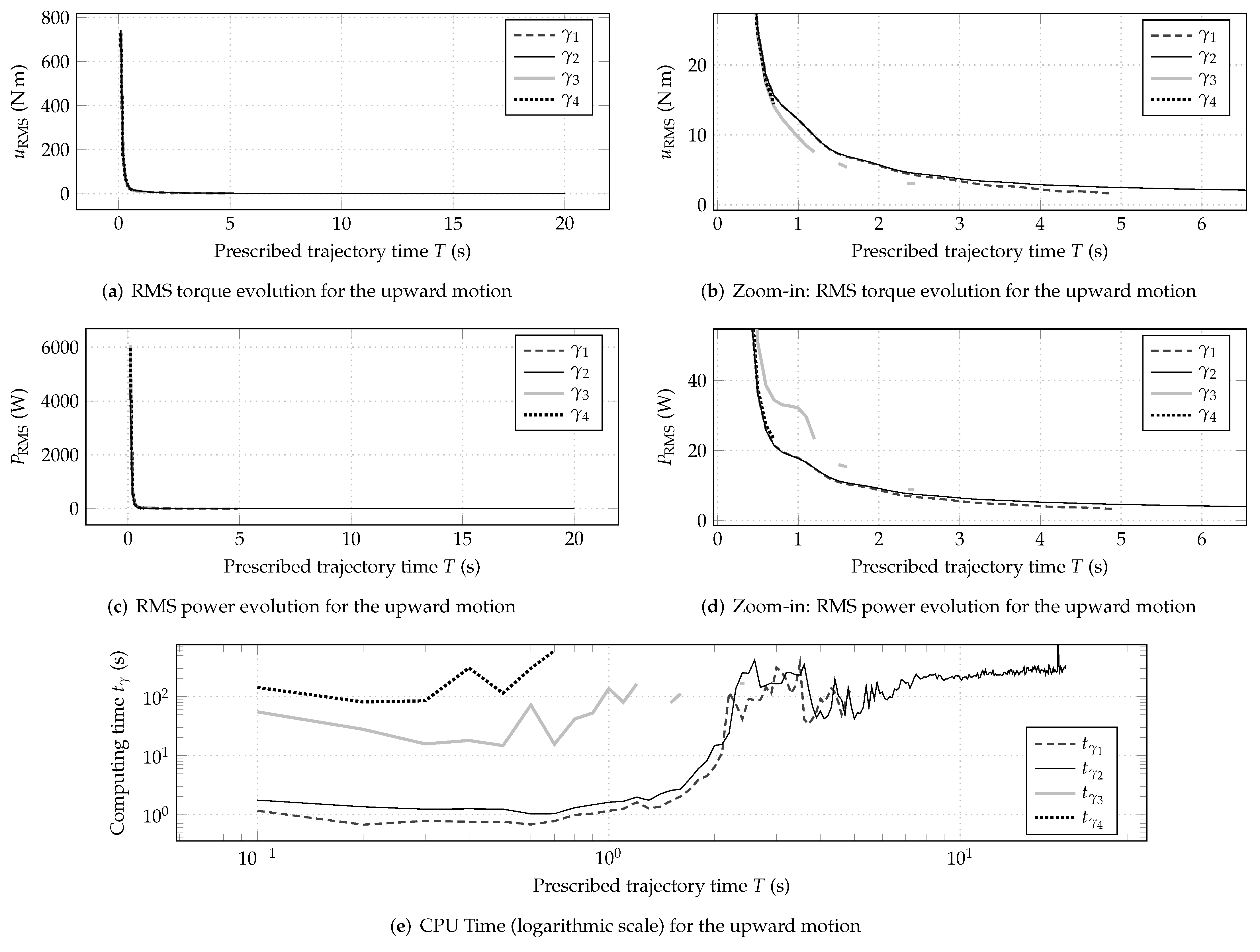
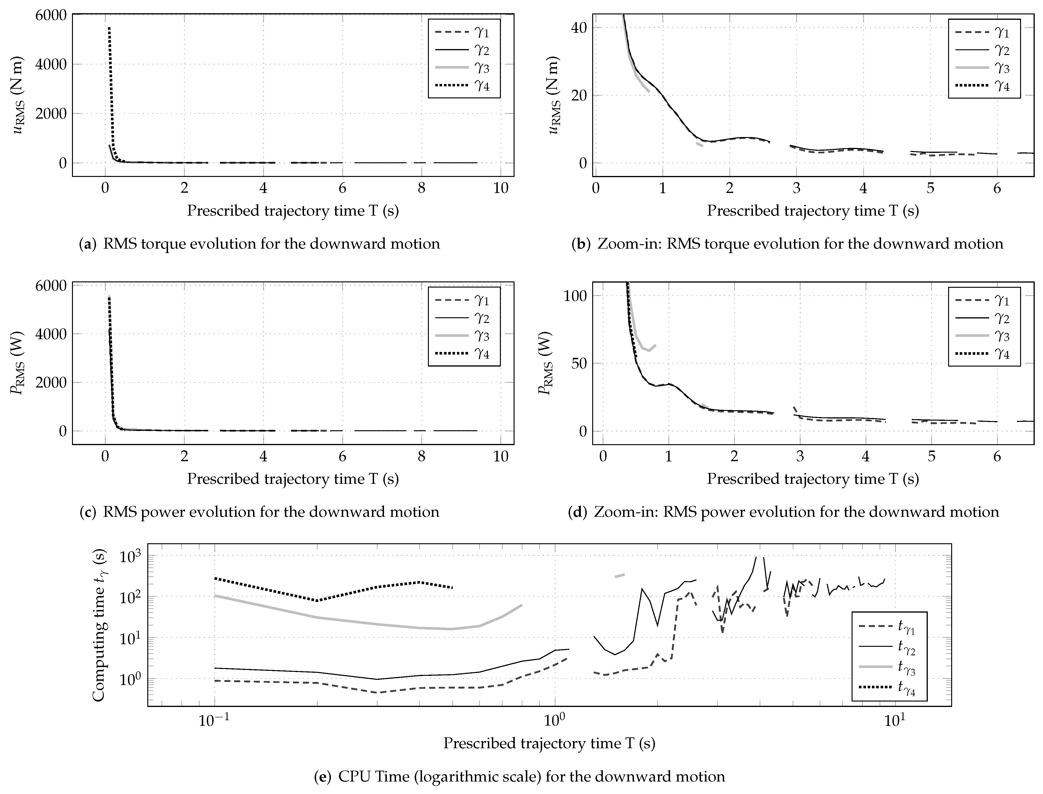
Compute the Root Mean Square (RMS) torque for each trajectory as

$$u_{\mathrm{RMS}}=\sqrt{\frac{{\int }_0^T{\sum }_{i=1}^n{u_i}^2}{T}}.$$

(55)

Step 3. 

Compute the RMS power for each trajectory as

$$P_{\mathrm{RMS}}=\sqrt{\frac{{\int }_0^T{\sum }_{i=1}^n{\left(u_i{\dot{q}}^i\right)}^2}{T}}.$$

(56)

Step 4. 

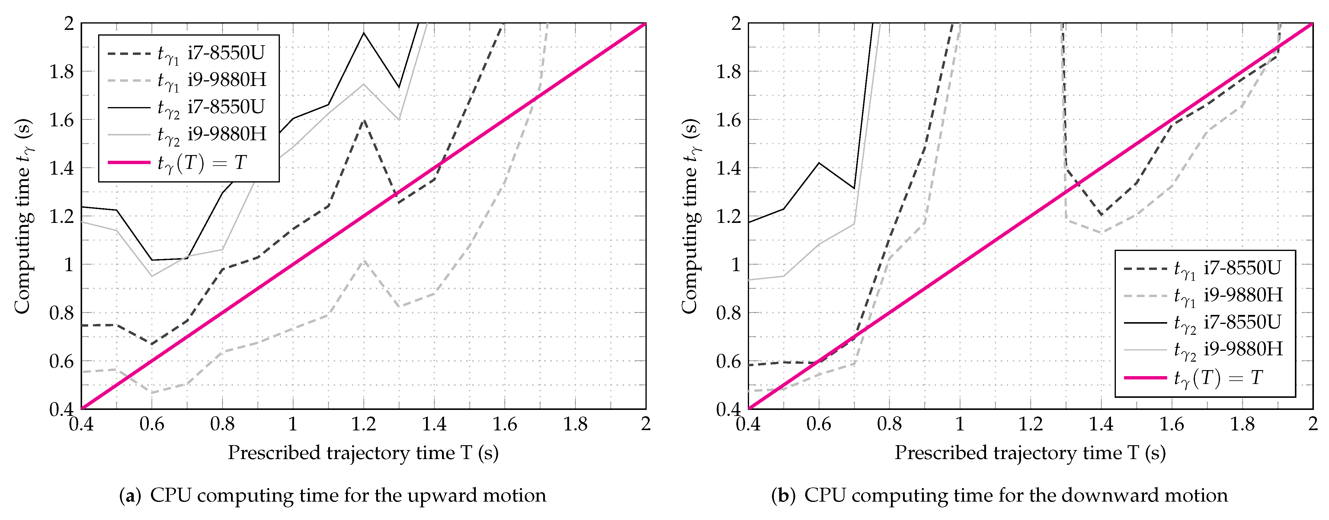
Determine the computation time for each trajectory.

Since our focus is on evaluating the impact of each cost function on the optimization process, a readily available ODE solver will be used to determine a solution to each of the encountered ODE systems. Wolfram Mathematica’s NDsolve ODE solver (version 12.3.1) was selected to perform these operations. This solver is able to function with a diversity of methods, among which shooting methods are found. This option would have been a natural candidate, but it was previously tried in [35], and the performance was not satisfactory. Instead, our results were obtained by calling the Runge–Kutta time integration method of NDSolve.

The time taken by the ODE solver to compute an optimal trajectory is referred to as computing time in our work. It is processor-dependent and determined using Mathematica’s AbsoluteTiming function. All simulations were held on a $1.8$ $\mathrm{G}$$\mathrm{Hz}$ 4-Core Intel Core i7 processor unless specified otherwise.

6.2. Results

The results of the above numerical trials will be presented and analyzed for an upward motion and a downward motion (see Step 1 of Section 6.1.3 above). Note that some results for the upward motion (Case (a)) were recently presented in the conference proceedings [43,44].

6.2.1. Increased Numerical Stability over Growing Values of T

Table 1 presents the maximum value of prescribed trajectory time T that NDSolve was able to reach with each of the four running cost functions that were tested. The table shows that our invariant running cost functions ${\gamma }_1$ and ${\gamma }_2$ are the ones that confer the solver an increased stability over extended prescribed trajectory times.

Table 1. Maximum prescribed times T for which NDSolve computes trajectories meeting conditions (53) and (54). The use of ${\gamma }_2$ allows the solver to reach higher values of T as compared to the other running cost functions. Note that both ${\gamma }_1$ and ${\gamma }_2$ are invariant; ${\gamma }_3$ and ${\gamma }_4$ are not.

Running Cost Function ${\mathit{\gamma }}_{\mathit{i}}$	Criterion	Maximum T Value for Upward Motion	Maximum T Value for Downward Motion
${\gamma }_1=\frac{1}{2}{u}^i{u}_i$	Torque	$4.9$$\mathrm{s}$	$5.7$$\mathrm{s}$
${\gamma }_2=\frac{1}{2}\left(u^i{u}_i+\alpha {\dot{q}}^i{\dot{q}}_i\right)$	Torque & velocity	$20.0$$\mathrm{s}$	$9.5$$\mathrm{s}$
${\gamma }_3=\frac{1}{2}{u}_i{u}_j$	Torque	$2.4$$\mathrm{s}$	$1.7$$\mathrm{s}$
${\gamma }_4=\frac{1}{2}\left(u_i{u}_j+{\dot{q}}^i{\dot{q}}^j\right)$	Torque & velocity	$0.7$$\mathrm{s}$	$0.5$$\mathrm{s}$

Simulation results are shown for the following: RMS torques in Figure 2a,b and Figure 3a,b; RMS power in Figure 2c,d and Figure 3c,d; and CPU computing time in Figure 2e and Figure 3e; each one was plotted versus the increasing prescribed time T. In order to better appreciate some results, Figure 2b,d show zoom-in versions of Figure 2a,c, respectively. In the same manner, Figure 3b,d are zoom-in versions of Figure 3a,c, respectively.

Figure 2. Upward motion (see Step 1 of Section 6.1.3): numerical solution of the optimal control of a two DOF robotic manipulator. Results for growing values of the prescribed trajectory time T: (a) RMS torque evolution; (b) cropped and zoomed-in version of (a); (c) RMS power evolution; (d) cropped and zoomed-in version of (c); (e) required time to compute a solution.Benefits of our invariant cost functions ${\gamma }_1$ and ${\gamma }_2$: lower RMS power values; improved solver stability with uninterrupted results up to $T=4.9\mathrm{s}$ for ${\gamma }_1$ and past $T=10\mathrm{s}$ for ${\gamma }_2$; substantially lower computing times.

Figure 3. Downward motion (see Step 1 of Section 6.1.3): numerical solution of the optimal control of a two DOF robotic manipulator. Results for growing values of the prescribed trajectory time T: (a) RMS torque evolution; (b) cropped and zoomed-in version of (a); (c) RMS power evolution; (d) cropped and zoomed-in version of (c); (e) required time to compute a solution. Benefits of our invariant cost functions ${\gamma }_1$ and ${\gamma }_2$: lower RMS power values; improved solver stability with uninterrupted results up to $T=5.7\mathrm{s}$ for ${\gamma }_1$ and up to $T=9.5\mathrm{s}$ for ${\gamma }_2$; substantially lower computing times.

First, note that not all curves attain the same prescribed time T. Let us begin with the upward motion. Only with ${\gamma }_2$ was NDSolve able to determine a solution up to $T=20$ s (see Table 1). Let us now focus on the case of ${\gamma }_3$. Curves corresponding to this running cost function display gaps because of numerical issues such as stiffness (which is quite common in similar cases [6]). This means that the solver is unable to compute a solution with ${\gamma }_3$ for certain trajectory durations T. Similar observations can be made for the downward motion: it is with ${\gamma }_2$ that the highest value of T was reached. However, this time, we see gaps in every curve because the solver struggles more than with the upward motion. Even so, robustness is still increased by using ${\gamma }_1$ and ${\gamma }_2$ instead of ${\gamma }_3$ and ${\gamma }_4$. These results confirm that our Riemannian formulation improves the solver stability with respect to the increasing prescribed times T.

6.2.2. RMS Torque, RMS Power, and CPU Computing Time

According to Figure 2a, which shows the evolution of RMS torques for the upward motion, lowest torque consumption is achieved with ${\gamma }_3$ followed by ${\gamma }_4$. However, according to Figure 2c, which shows the evolution of RMS power for the upward motion, the lowest power consumption is achieved with ${\gamma }_1$ followed by ${\gamma }_2$. The same observations can be made for the downward motion (see Figure 3).

Then, we have compared computing times $t_{{\gamma }_i}$ between similar running cost functions—${\gamma }_1$ and ${\gamma }_3$ use a torque criterion; ${\gamma }_2$ and ${\gamma }_4$ use a torque plus velocity criterion—by calculating the ratios between such times. These ratios are reported in Table 2 and characterize the performance increase resulting from our formulation in terms of CPU computing time. In other words, they quantify how the solver was able to determine a solution a number of times faster with the invariant running cost functions than with the non-invariant ones. We have also performed our tests on a $2.3$ $\mathrm{G}$$\mathrm{Hz}$ 8-Core Intel Core i9 processor to get additional computing times (processor-dependent).

Table 2. NDSolve computing time decrease factor: ratio between comparable running cost functions. The decrease in computing time resulting from our invariant running cost functions ${\gamma }_1$ and ${\gamma }_2$ is noticeable.

Motion	Upward		Upward		Downward		Downward
Ratio	$\raisebox{1ex}{${\mathit{t}}_{{\mathit{\gamma }}_3}$}\!\left/ \!\raisebox{-1ex}{${\mathit{t}}_{{\mathit{\gamma }}_1}$}\right.$ (Torque)		$\raisebox{1ex}{${\mathit{t}}_{{\mathit{\gamma }}_4}$}\!\left/ \!\raisebox{-1ex}{${\mathit{t}}_{{\mathit{\gamma }}_2}$}\right.$ (Torque and Velocity)		$\raisebox{1ex}{${\mathit{t}}_{{\mathit{\gamma }}_3}$}\!\left/ \!\raisebox{-1ex}{${\mathit{t}}_{{\mathit{\gamma }}_1}$}\right.$ (Torque)		$\raisebox{1ex}{${\mathit{t}}_{{\mathit{\gamma }}_4}$}\!\left/ \!\raisebox{-1ex}{${\mathit{t}}_{{\mathit{\gamma }}_2}$}\right.$ (Torque and Velocity)
Processor	i7-8550U	i9-9880H	i7-8550U	i9-9880H	i7-8550U	i9-9880H	i7-8550U	i9-9880H
Base Value	4	5	60	55	18	29	56	57
Average	51	73	205	138	99	85	142	146

According to these results, our formulation enables a considerable CPU time decrease. In particular, let us take the computing times $t_{\gamma }\left(T\right)$ required by our two processors to solve our optimal control exercise using ${\gamma }_1$ and ${\gamma }_2$, restrict the prescribed trajectory time window between $0.4$ and 2 $\mathrm{s}$, and plot such values. Figure 4 shows these curves for both the upward and the downward motion. Note that the values that remain below the solid straight line correspond to CPU computing times for which $t_{\gamma }\left(T\right)<T$. Optimal trajectories for which this is the case take less time to compute than the time T they require to complete. In other words, for some of these prescribed time T values, not only could real-time optimal control eventually be considered but also motion replanning.

Figure 4. CPU computing time required to obtain a solution with ${\gamma }_1$ and ${\gamma }_2$. Results for two processors: Intel i7-8550U and Intel i9-9880H on a prescribed trajectory time window comprised between $0.4$ and 2 $\mathrm{s}$. Values that remain below the solid straight line correspond to optimal trajectories that take less time to compute than they require to complete ($t_{\gamma }\left(T\right)<T$). Real-time optimal control or motion replanning could be considered in these cases.

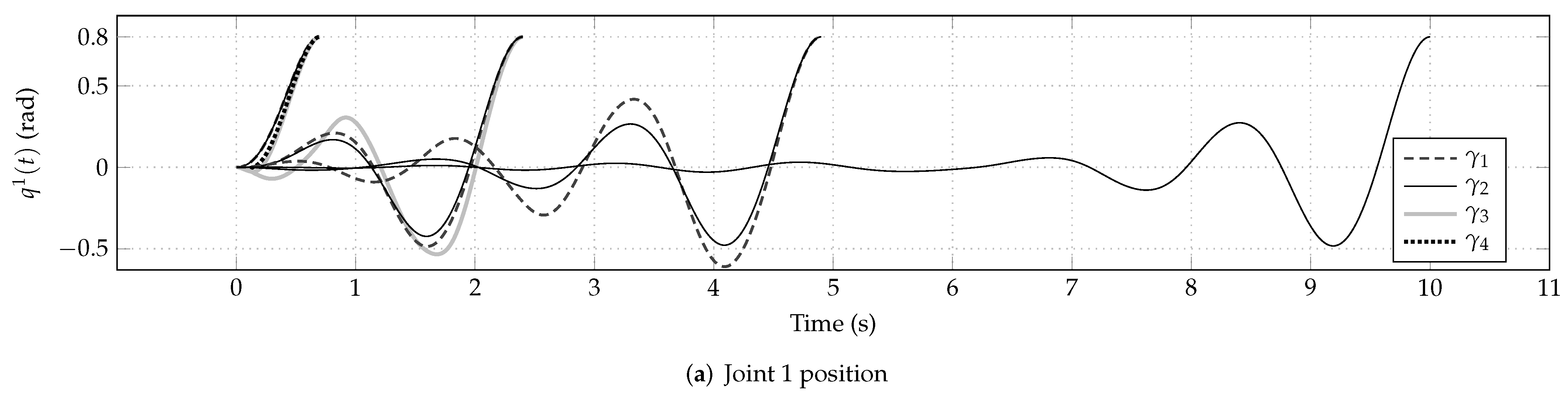
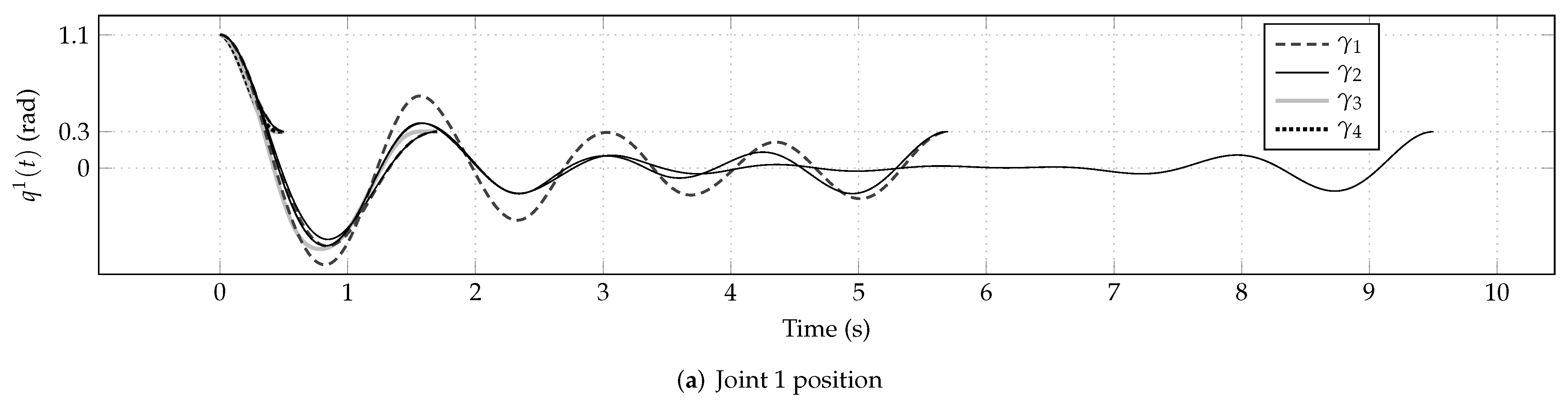
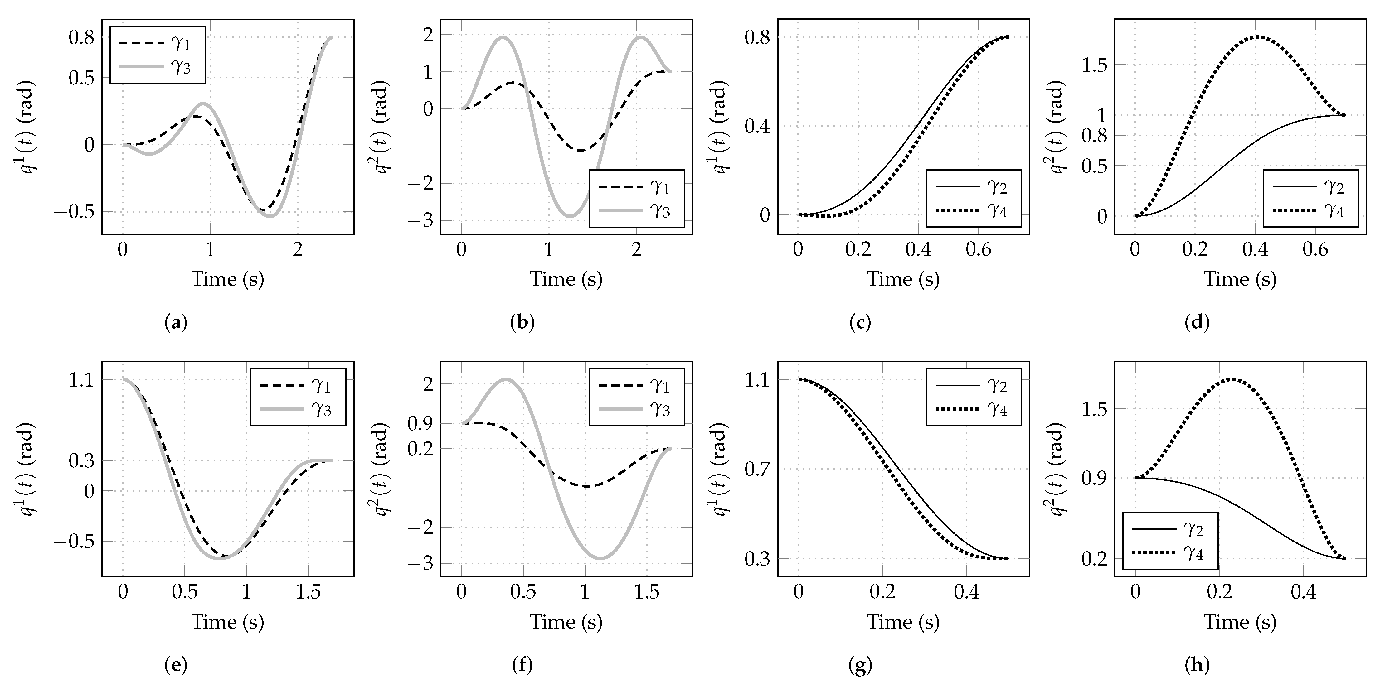
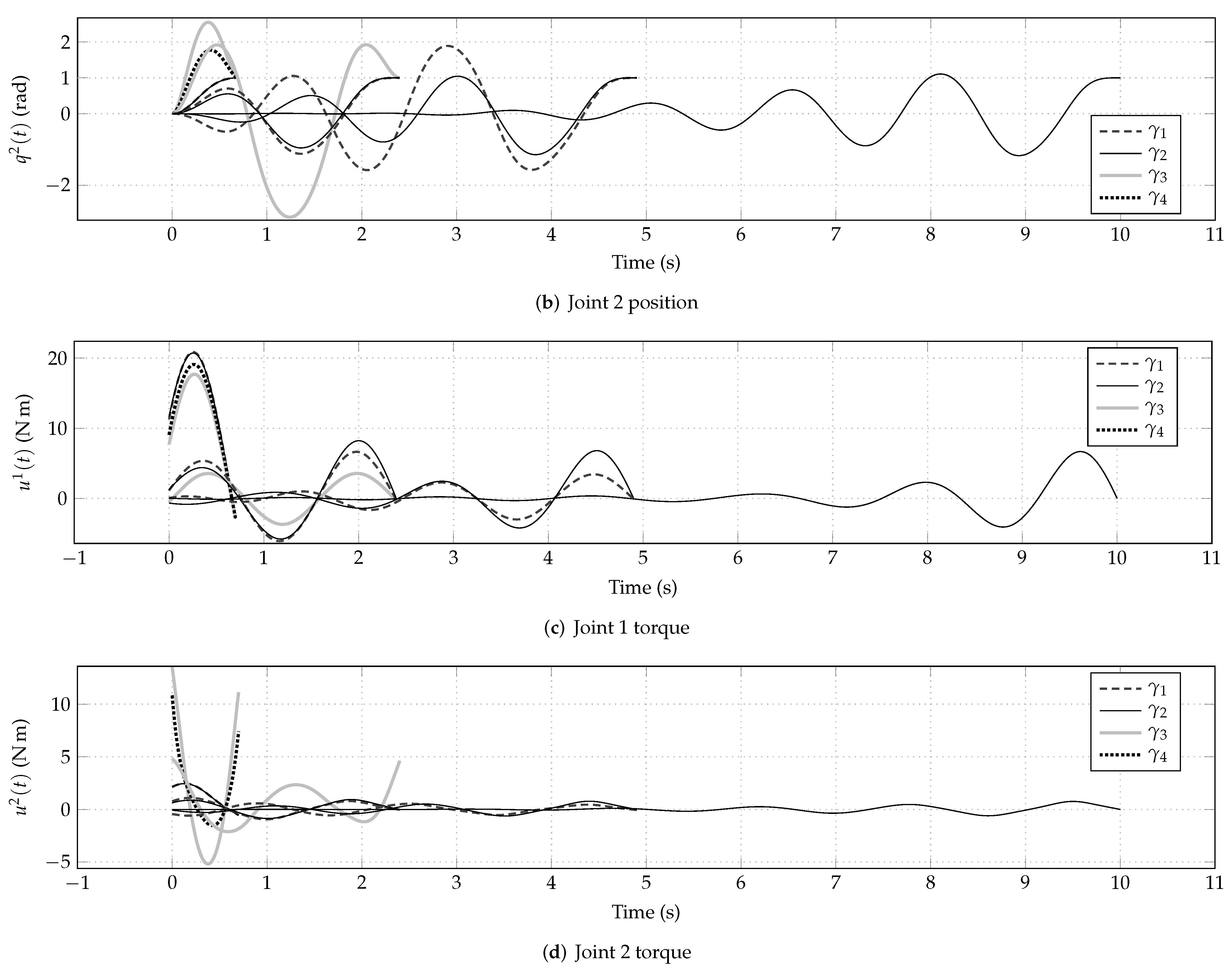
6.2.3. Observed Motion Characteristics

We now compare the results obtained with running cost functions that share similarities in their criteria. We focus on the trajectory positions in order to analyze motion characteristics. According to Figure 5, the invariant running cost functions ${\gamma }_1$ and ${\gamma }_2$ stabilize motion by narrowing the overall angular amplitude during the trajectory. This is valid for either the upward or the downward motion.

Figure 5. Comparison of positions along optimal trajectories, resulting from invariant running cost functions (${\gamma }_1$ and ${\gamma }_2$) versus non-invariant ones (${\gamma }_3$ and ${\gamma }_4$). Functions ${\gamma }_1$ and ${\gamma }_3$ share a torque criterion; functions ${\gamma }_2$ and ${\gamma }_4$ share a torque plus velocity criterion. The invariant running cost functions stabilize motion by narrowing angular amplitude. (a) Joint 1 positions with ${\gamma }_1$ and ${\gamma }_3$ for the upward motion. (b) Joint 2 positions with ${\gamma }_1$ and ${\gamma }_3$ for the upward motion. (c) Joint 1 positions with ${\gamma }_2$ and ${\gamma }_4$ for the upward motion. (d) Joint 2 positions with ${\gamma }_2$ and ${\gamma }_4$ for the upward motion. (e) Joint 1 positions with ${\gamma }_1$ and ${\gamma }_3$ for the downward motion. (f) Joint 2 positions with ${\gamma }_1$ and ${\gamma }_3$ for the downward motion. (g) Joint 1 positions with ${\gamma }_2$ and ${\gamma }_4$ for the downward motion. (h) Joint 2 positions with ${\gamma }_2$ and ${\gamma }_4$ for the downward motion.

For further analysis, consider Figure 6 and Figure 7, which show the curves of optimal torque and position along trajectories for the upward and downward motion. We have selected four simulated trajectories for T = $0.7$ $\mathrm{s}$, T = $2.4$ $\mathrm{s}$, T = $4.9$ $\mathrm{s}$, and T = 10 $\mathrm{s}$ (upward motion); T = $0.5$ $\mathrm{s}$, T = $1.7$ $\mathrm{s}$, T = $5.7$ $\mathrm{s}$ and T = $9.5$ $\mathrm{s}$ (downward motion). These values of T correspond to those of Table 1, which are the maximum values at which NDSolve successfully determined a solution with the exception of T = 10 $\mathrm{s}$ for the upward motion with ${\gamma }_2$, which was selected to improve curve readability.

Figure 6. Numerical solution of the optimal control for an upward motion (see Step 1 of Section 6.1.3). Optimal torque and position evolution along four simulated trajectories: T = $0.7$$\mathrm{s}$, T = $2.4$$\mathrm{s}$, T = $4.9$$\mathrm{s}$, and T = 10 $\mathrm{s}$. Trajectory durations correspond to values of T in Table 1, which are the maximum values at which NDSolve successfully determined a solution with the exception of T = 1 $\mathrm{s}$ for ${\gamma }_2$. Higher values of T and narrower motions are achieved with the invariants ${\gamma }_1$ and ${\gamma }_2$.

Figure 7. Numerical solution of the optimal control for a downward motion (see Step 1 of Section 6.1.3). Optimal torque and position evolution along four simulated trajectories: T = $0.5$$\mathrm{s}$, T = $1.7$$\mathrm{s}$, T = $5.7$$\mathrm{s}$, and T = $9.5$$\mathrm{s}$. Trajectory durations correspond to values of T in Table 1, which are the maximum values at which NDSolve successfully determined a solution. Higher values of T and narrower motions are achieved with the invariants ${\gamma }_1$ and ${\gamma }_2$.

Note that as T increases, a similar tendency can be observed with each running cost function. Positions oscillate toward and around the goal. However, as previously shown, oscillations tend to be narrower with our invariant running cost functions ${\gamma }_1$ and ${\gamma }_2$ than with their non-invariant counterparts ${\gamma }_3$ and ${\gamma }_4$. Torques oscillate in a similar fashion but around zero because torque consumption is being minimized.

7. Conclusive Remarks

This paper presented a Riemannian formulation of Pontryagin’s maximum principle for the optimal control of robotic manipulators where an invariant running cost function was selected under the criteria of torque and energy minimization. The presented optimal control methodology is an indirect method where the problem becomes that of solving a first-order system of ODE, which is contravariant in the states and covariant in the co-states.

By regarding the running cost as a function of the configuration parameter and its first and second time derivatives, Euler–Lagrange equations are applied. This results in a time evolution equation for the optimal torque, which is a covariant of the second order (see Proposition 1). These equations feature the Riemann curvature tensor and are addressed to as the covariant control equations.

Then, by applying Pontryagin’s maximum principle, it is further proved that the adjoint variables are in fact a first-order representation of the second-order covariant control equations mentioned above (see Proposition 3). This establishes an equivalence between the application of the Euler–Lagrange equations and Pontryagin’s maximum principle for our problem, which is made possible with the choice of our invariant running cost functions. A physical interpretation is also provided for one of the adjoint variables, which turns out to be exactly the required torque to cause motion. This means that further calculations are unnecessary in order to retrieve this physical quantity, which is needed for torque control.

Finally, the impact of our Riemannian formulation on a commercial ODE solver was briefly examined. Since the analyses in this document were enabled by the choice of invariant running cost functions, controlled motion simulations were conducted on a robotic manipulator for which four running cost functions were evaluated. Two non-invariant running cost functions (${\gamma }_3$ and ${\gamma }_4$) were compared with our invariant running cost functions (${\gamma }_1$ and ${\gamma }_2$). Then, their effect on the resulting robot motion and on a commercial ODE solver was examined. From the numerical perspective, our formulation provides these interesting benefits:

• efficient motions requiring less power (see Figure 2c and Figure 3c);
• faster operation of the ODE solver resulting in shorter computing times (see Figure 2e and Figure 3e, and Table 2);
• improved stability of the ODE solver with respect to trajectory time T (see Table 1 and Figure 2, Figure 3, Figure 6 and Figure 7);
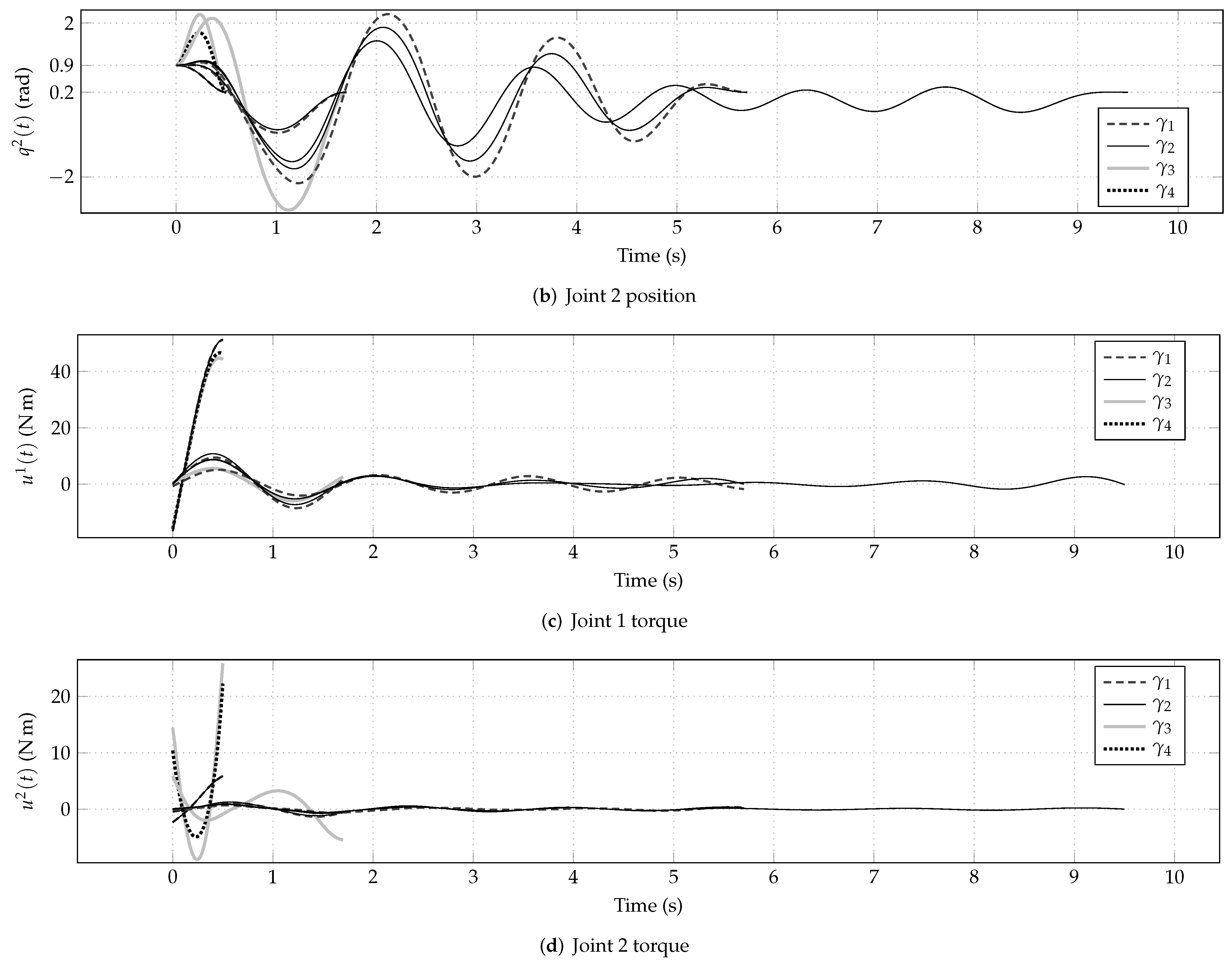
• narrower joint motions (see Figure 5).

Additionally, it has come to our attention that some of the obtained optimal trajectories could be considered for real-time optimal control or even motion replanning (see Figure 4). This results from the substantial decrease in computing time, which is made possible with our formulation.

The presented method is currently devoted to compute the optimal positions and torques along a trajectory on the premise that a tracking controller ensures that the optimal path is being followed by the robot. However, our method could be enhanced by considering tracking and output feedback. In future developments, this could enable an online optimal control strategy.

Our proposal conjugates geometry with principles of minimum force and minimum energy (as it is recommended in [26]). The result is an efficient and robust way to plan for the optimal motion of robotic manipulators. As an outlook, we recall that our proposed running cost function ${\gamma }_2$ combines torque and energy policies. In order to preserve homogeneity in this combination, a scaling factor $\alpha$ had to be used. This number was set to be unitary for the sake of generality in this work. However, this factor provides a supplementary DOF to the running cost function. Therefore, we shall analyze the effects of a variable $\alpha$ in future research.

References

- Benallegue, M.; Laumond, J.P.; Mansard, N. Springer Tracts in Advanced Robotics, Chapter Robot Motion Planning and Control: Is It More Than a Technological Problem? In Geometric and Numerical Foundations of Movements; Springer: Cham, Switzerland, 2017; Volume 117. [Google Scholar] [CrossRef]
- Latombe, J.C. Robot Motion Planning; The Springer International Series in Engineering and Computer Science; Springer: Boston, MA, USA, 1991. [Google Scholar] [CrossRef]
- Siciliano, B.; Sciavicco, L.; Villani, L.; Oriolo, G. Robotics: Modeling, Planning and Control; Advanced Textbooks in Control and Signal Processing; Springer: London, UK, 2009. [Google Scholar] [CrossRef]
- Craig, J.J. Introduction to Robotics: Mechanics and Control, 4th ed.; Pearson Education Limited: Harlow, UK, 2018. [Google Scholar]
- Spong, M.; Hutchinson, S.; Vidyasagar, M. Robot Modeling and Control, 2nd ed.; John Wiley and Sons: Hoboken, NJ, USA, 2020. [Google Scholar]
- Grancharova, A.; Johansen, T.A. Survey of Explicit Approaches to Constrained Optimal Control. In Switching and Learning in Feedback Systems; Murray-Smith, R., Shorten, R., Eds.; Springer: Berlin/Heidelberg, Germany, 2005; pp. 47–97. [Google Scholar] [CrossRef]
- Betts, J.T. Practical Methods for Optimal Control and Estimation Using Nonlinear Programming, 2nd ed.; Society for Industrial and Applied Mathematics: Philadelphia, PA, USA, 2010. [Google Scholar] [CrossRef]
- Pontryagin, L.S.; Boltyanskii, V.G.; Gamkrelidze, R.V.; Mishchenko, E.F. The Mathematical Theory of Optimal Processes; Interscience Publishers (Division of John Wiley & Sons, Inc.): New York, NY, USA, 1962. [Google Scholar]
- Mesterton-Gibbons, M. A Primer on the Calculus of Variations and Optimal Control Theory; American Mathematical Society: Providence, RI, USA, 2009; Volume 50. [Google Scholar] [CrossRef]
- Liberzon, D. Calculus of Variations and Optimal Control Theory: A Concise Introduction; Princeton University Press: Princeton, NJ, USA, 2012. [Google Scholar]
- Nikoobin, A.; Moradi, M. Optimal balancing of robot manipulators in point-to-point motion. Robotica 2011, 29, 233–244. [Google Scholar] [CrossRef]
- Boscariol, P.; Richiedei, D. Robust point-to-point trajectory planning for nonlinear underactuated systems: Theory and experimental assessment. Robot. Comput. Integr. Manuf. 2018, 50, 256–265. [Google Scholar] [CrossRef]
- Crain, A.; Ulrich, S. Experimental Validation of Pseudospectral-Based Optimal Trajectory Planning for Free-Floating Robots. J. Guid. Control Dyn. 2019, 42, 1726–1742. [Google Scholar] [CrossRef] [Green Version]
- Putkaradze, V.; Rogers, S. On the Optimal Control of a Rolling Ball Robot Actuated by Internal Point Masses. J. Dyn. Syst. Meas. Control 2020, 142, 051002. [Google Scholar] [CrossRef] [Green Version]
- Vezvari, M.R.; Nikoobin, A.; Ghoddosian, A. Zero-power balancing a two-link robot manipulator for a predefined point-to-point task. J. Mech. Sci. Technol. 2020, 34, 2585–2595. [Google Scholar] [CrossRef]
- Sciavicco, L.; Siciliano, B. Modelling and Control of Robot Manipulators, 2nd ed.; Advanced Textbooks in Control and Signal Processing; Springer: London, UK, 2000. [Google Scholar] [CrossRef]
- Pan, H.; Xin, M. Nonlinear robust and optimal control of robot manipulators. Nonlinear Dyn. 2014, 76, 237–254. [Google Scholar] [CrossRef]
- Ott, C.; Eiberger, O.; Friedl, W.; Bauml, B.; Hillenbrand, U.; Borst, C.; Albu-Schaffer, A.; Brunner, B.; Hirschmuller, H.; Kielhofer, S.; et al. A Humanoid Two-Arm System for Dexterous Manipulation. In Proceedings of the IEEE-RAS International Conference on Humanoid Robots, Genova, Italy, 4–6 December 2006; pp. 276–283. [Google Scholar] [CrossRef]
- Busch, B.; Cotugno, G.; Khoramshahi, M.; Skaltsas, G.; Turchi, D.; Urbano, L.; Wächter, M.; Zhou, Y.; Asfour, T.; Deacon, G.; et al. Evaluation of an Industrial Robotic Assistant in an Ecological Environment. In Proceedings of the 2019 28th IEEE International Conference on Robot and Human Interactive Communication (RO-MAN), New Delhi, India, 14–18 October 2019; pp. 1–8. [Google Scholar] [CrossRef]
- Spong, M. Remarks on robot dynamics: Canonical transformations and Riemannian geometry. In Proceedings of the 1992 IEEE International Conference on Robotics and Automation, Nice, France, 12–14 May 1992; Volume 1, pp. 554–559. [Google Scholar] [CrossRef]
- Park, F.; Bobrow, J.; Ploen, S. A Lie Group Formulation of Robot Dynamics. Int. J. Robot. Res. 1995, 14, 609–618. [Google Scholar] [CrossRef]
- Stokes, A.; Brockett, R. Dynamics of Kinematic Chains. Int. J. Robot. Res. 1996, 15, 393–405. [Google Scholar] [CrossRef]
- Park, F.; Choi, J.; Ploen, S. Symbolic formulation of closed chain dynamics in independent coordinates. Mech. Mach. Theory 1999, 34, 731–751. [Google Scholar] [CrossRef]
- Žefran, M.; Bullo, F. Robotics and Automation Handbook; Chapter Lagrangian Dynamics; CRC Press: Boca Raton, FL, USA, 2005. [Google Scholar]
- Gu, Y.L. Modeling and simplification for dynamic systems with testing procedures and metric decomposition. In Proceedings of the Conference Proceedings 1991 IEEE International Conference on Systems, Man, and Cybernetics, Charlottesville, VA, USA, 13–16 October 1991; Volume 1, pp. 487–492. [Google Scholar] [CrossRef]
- Bennequin, D.; Berthoz, A. Springer Tracts in Advanced Robotics, Chapter Several Geometries for Movements Generations. In Geometric and Numerical Foundations of Movements; Springer: Cham, Switzerland, 2017; Volume 117. [Google Scholar] [CrossRef]
- Athans, M.; Falb, P.L. Optimal Control: An Introduction to the Theory and Its Applications; Dover Books on Engineering; Dover Publications: New York, NY, USA, 2006. [Google Scholar]
- Lovelock, D.; Rund, H. Tensors, Differential Forms, and Variational Principles; Dover Books on Mathematics; Dover Publications: New York, NY, USA, 1989. [Google Scholar]
- Grinfeld, P. Introduction to Tensor Analysis and the Calculus of Moving Surfaces; Springer: New York, NY, USA, 2013. [Google Scholar] [CrossRef]
- Goldstein, H.; Poole, C.; Safko, J. Classical Mechanics; Addison-Wesley Series in Physics; Addison Wesley: New York, NY, USA, 2002. [Google Scholar]
- Dubois, F.; Fortuné, D.; Rojas Quintero, J.A.; Vallée, C. Pontryagin Calculus in Riemannian Geometry. In Geometric Science of Information; Nielsen, F., Barbaresco, F., Eds.; Springer International Publishing: Cham, Switzerland, 2015; pp. 541–549. [Google Scholar] [CrossRef]
- Rojas-Quintero, J.A.; Rojas-Estrada, J.A.; Villalobos-Chin, J.; Santibañez, V.; Bugarin, E. Optimal controller applied to robotic systems using covariant control equations. Int. J. Control 2021, 1–14. [Google Scholar] [CrossRef]
- Rojas-Quintero, J.A. Contribution à la Manipulation Dextre Dynamique Pour les Aspects Conceptuels et de Commande en Ligne Optimale [French]. Ph.D. Thesis, Université de Poitiers, Poitiers, France, 2013. [Google Scholar]
- Almuslimani, I.; Vilmart, G. Explicit Stabilized Integrators for Stiff Optimal Control Problems. SIAM J. Sci. Comput. 2021, 43, A721–A743. [Google Scholar] [CrossRef]
- Rojas-Quintero, J.A.; Villalobos-Chin, J.; Santibanez, V. Optimal Control of Robotic Systems Using Finite Elements for Time Integration of Covariant Control Equations. IEEE Access 2021, 9, 104980–105001. [Google Scholar] [CrossRef]
- Reyes Cortés, F.; Kelly, R. Experimental evaluation of model-based controllers on a direct-drive robot arm. Mechatronics 2001, 11, 267–282. [Google Scholar] [CrossRef]
- Berret, B.; Chiovetto, E.; Nori, F.; Pozzo, T. Evidence for composite cost functions in arm movement planning: An inverse optimal control approach. PLoS Comput. Biol. 2011, 7, e1002183. [Google Scholar] [CrossRef] [PubMed]
- Kaphle, M.; Eriksson, A. Optimality in forward dynamics simulations. J. Biomech. 2008, 41, 1213–1221. [Google Scholar] [CrossRef] [PubMed]
- Martin, B.J.; Bobrow, J.E. Minimum-Effort Motions for Open-Chain Manipulators with Task-Dependent End-Effector Constraints. Int. J. Robot. Res. 1999, 18, 213–224. [Google Scholar] [CrossRef]
- Eriksson, A. Temporal finite elements for target control dynamics of mechanisms. Comput. Struct. 2007, 85, 1399–1408. [Google Scholar] [CrossRef]
- Kelly, M. An Introduction to Trajectory Optimization: How to Do Your Own Direct Collocation. SIAM Rev. 2017, 59, 849–904. [Google Scholar] [CrossRef]
- Eriksson, A.; Nordmark, A. Temporal finite element formulation of optimal control in mechanisms. Comput. Methods Appl. Mech. Eng. 2010, 199, 1783–1792. [Google Scholar] [CrossRef]
- Morales-López, S.; Rojas-Quintero, J.A.; Ramírez-de Ávila, H.C.; Bugarin, E. Evaluation of invariant cost functions for the optimal control of robotic manipulators. In Proceedings of the 2021 9th International Conference on Systems and Control (ICSC), Caen, France, 24–26 November 2021; pp. 350–355. [Google Scholar] [CrossRef]
- Ramírez-de Ávila, H.C.; Rojas-Quintero, J.A.; Morales-López, S.; Bugarin, E. Comparing cost functions for the optimal control of robotic manipulators using Pontryagin’s Maximum Principle. In Proceedings of the 2021 XXIII Robotics Mexican Congress (ComRob), Tijuana, Mexico, 27–29 October 2021; pp. 106–111. [Google Scholar] [CrossRef]
Publisher’s Note: MDPI stays neutral with regard to jurisdictional claims in published maps and institutional affiliations. |
© 2022 by the authors. Licensee MDPI, Basel, Switzerland. This article is an open access article distributed under the terms and conditions of the Creative Commons Attribution (CC BY) license (https://creativecommons.org/licenses/by/4.0/).