Circumventing Ill-Conditioning Arising from Using Linear Multistep Methods in Approximating the Solution of Initial Value Problems

Abstract

When finding numerical solutions to stiff and nonstiff initial value problems using linear multistep methods, ill-conditioned systems are often encountered. In this paper, we demonstrate how this ill-conditioning can be circumvented without iterative refinement or preconditioning, by carefully choosing the grid point used in deriving the discrete scheme from the continuous formulation. Results of numerical experiments show that the new scheme perform very well when compared with the exact solution and results from an earlier scheme.

1. Introduction

According to Shampine [1], matrices derived from the solution of stiff initial value problems using linear multistep methods (LMMs) are almost always ill-conditioned. In this article, we show that these ill-conditioned systems can be made well- or better-conditioned. In an attempt to find numerical approximations to the initial value problem $y^{\prime }=-y$ with initial condition $y_o=1$ using the two-step Butcher’s hybrid scheme in block form by Akinola and Ajibade [2], it was discovered that by interpolating at the grid point $x=x_{n+\frac{7}{4}}$, the condition number of the resultant linear system of equations was large. The goal in this present work is to find ways in which this condition number can be reduced so that we can solve a better-conditioned system without compromising accuracy. According to [3], a matrix $\mathbf{A}$ is well-conditioned if its condition number $\kappa \left(\mathbf{A}\right)$ is close to 1 and ill-conditioned if the condition number $\kappa \left(\mathbf{A}\right)$ is significantly greater than 1. This implies that, if $\mathbf{A}$ is well-conditioned, then small changes in $\mathbf{A}$ and $\mathbf{b}$ result in corresponding small changes in $\mathbf{x}$. In the same vein, if $\mathbf{A}$ is ill-conditioned, then small changes in $\mathbf{A}$ and $\mathbf{b}$ produce large changes in the solution vector $\mathbf{x}$ [4] (see also, [5,6,7,8]). The approach we adopt to achieve our aim is threefold: instead of interpolating at $x=x_{n+\frac{7}{4}}$, we rather interpolate at $x=x_{n+\frac{5}{2}}$ on the one hand and solved an underdetermined system of linear equations involving two equations in four unknowns on the other hand, using the same grid point. The former involves solving a square system of linear equations. In [2], a theorem was proved that gives a condition for the nonsingularity of the $\mathbf{D}$ matrix used in deriving the continuous formulation of the two-step Butcher’s hybrid scheme in block form, in this paper, we also consider different values of the step sizes h for which the $\mathbf{D}$ matrix is singular, nearly singular and nonsingular to see if these affects the condition number of the matrix or solution obtained from the resulting discrete schemes.

In a closely related work by [2,9,10], the authors solved the resultant ill-conditioned system of equations without mentioning how this could be circumvented. We make it clear at this juncture that we do not lay claim to be the first to provide ways in which the solution of an ill-conditioned linear system of equations can be overcome [11]. Rather, we state how to reduce the condition number of ill-conditioned linear systems arising from LMMs for solving stiff and nonstiff initial value problems without preconditioning.

Skwame et al. [12], derived two continuous schemes from which, by interpolating at different grid points $x=x_{n+1},x=x_{n+2},x=x_{n+3},x=x_{n+4},x=x_{n+\frac{9}{2}}$ and $x=x_{n+5}$, they obtained a seventh-order block hybrid LMMs, on the one hand, and an eighth-order block hybrid LMMs, on the other. These methods were applied on some stiff initial value problems without a discussion on the ill-conditioning of the corresponding system of equations. This might be one of the reasons why the result of their numerical experiments was not good. Other literature works in which the authors did not bother to examine ill-conditioning are [13,14,15,16,17,18,19,20,21] and the references therein. It is worthy of note that Mohammed et al., in [22,23,24], provided numerical schemes based on hybrid methods for the solution of second- and third-order IVPs approximating at various grid points without discussing the steps taken to avoid solving an ill-conditioned system. This was followed by the works of [25,26,27,28,29,30,31,32,33,34,35,36,37,38,39,40] in which the authors overlooked ill-conditioning. The plan of this work is as follows: in Section 2 we present the D matrix used in this work as well as derive all the discrete schemes. Convergence analyses of the schemes is analysed in Section 3 and we bring this work to a close with some numerical experiments in Section 4.

2. Materials and Methods

The matrix $\mathbf{D}$ used in deriving the continuous scheme in [2] is

$$\mathbf{D}=\left[\begin{array}{cccccc}1& x_n& x_n^2& x_n^3& x_n^4& x_n^5\\ \\ 1& x_{n+1}& x_{n+1}^2& x_{n+1}^3& x_{n+1}^4& x_{n+1}^5\\ \\ 0& 1& 2x_n& 3x_n^2& 4x_n^3& 5x_n^4\\ \\ 0& 1& 2x_{n+1}& 3x_{n+1}^2& 4x_{n+1}^3& 5x_{n+1}^4\\ \\ 0& 1& 2x_{n+2}& 3x_{n+2}^2& 4x_{n+2}^3& 5x_{n+2}^4\\ \\ 0& 1& 2x_{n+\frac{3}{2}}& 3x_{n+\frac{3}{2}}^2& 4x_{n+\frac{3}{2}}^3& 5x_{n+\frac{3}{2}}^4\end{array}\right].$$

(1)

The above matrix was shown to be nonsingular in [2] if the step size h is not too small and we state the theorem without proof.

Theorem 1.

If the step size h is not too small, then $\mathbf{D}$ given by (1) is nonsingular.

Proof. 

See [2]. □

The following continuous scheme was discussed in [2,10]

$$\begin{array}{cc}\hfill \overline{y}\left(x\right)& =\left[\frac{-24{\omega }^5-15h{\omega }^4+40h^2{\omega }^3+30h^3{\omega }^2}{31h^5}\right]y_n+\left[\frac{24{\omega }^5+15h{\omega }^4-40h^2{\omega }^3-30h^3{\omega }^2+31h^5}{31h^5}\right]y_{n+1}\hfill \\ \\ \hfill & +\left[\frac{-96{\omega }^5-91h{\omega }^4+98h^2{\omega }^3+89h^3{\omega }^2}{372h^4}\right]f_n+\left[\frac{-28{\omega }^5-2h{\omega }^4+57h^2{\omega }^3+4h^3{\omega }^2-31h^4\omega }{31h^4}\right]f_{n+1}\hfill \\ \\ \hfill & +\left[\frac{-16{\omega }^5+21h{\omega }^4+6h^2{\omega }^3-11h^3{\omega }^2}{124h^4}\right]f_{n+2}+\left[\frac{48{\omega }^5-32h{\omega }^4-80h^2{\omega }^3+64h^3{\omega }^2}{93h^4}\right]f_{n+\frac{3}{2}}.\hfill \end{array}$$

(2)

If we evaluate (2) at $\omega =-h,\omega =-\frac{h}{2},\omega =-\frac{3h}{4}$ and its derivative at $\omega =-\frac{3h}{4}$, then

$$\begin{array}{ccc}\hfill y_{n+2}& =& -\frac{1}{31}{y}_n+\frac{32}{31}{y}_{n+1}+\frac{h}{93}\left[-f_n+12f_{n+1}+64f_{n+\frac{3}{2}}+15f_{n+2}\right]\hfill \end{array}$$

(3)

$$\begin{array}{ccc}\hfill y_{n+\frac{3}{2}}& =& \frac{37}{496}{y}_n+\frac{459}{496}{y}_{n+1}+\frac{h}{1984}\left[39f_n+648f_{n+1}+480f_{n+\frac{3}{2}}-27f_{n+2}\right]\hfill \end{array}$$

(4)

$$\begin{array}{ccc}\hfill y_{n+\frac{7}{4}}& =& \frac{243}{7936}{y}_n+\frac{7693}{7936}{y}_{n+1}+\frac{h}{31744}\left[231f_n+7644f_{n+1}+16464f_{n+\frac{3}{2}}+441f_{n+2}\right]\hfill \end{array}$$

(5)

$$\begin{array}{ccc}\hfill -\frac{315}{992}{y}_{n+1}& =& -\frac{315}{992}{y}_n+\frac{h}{1984}\left[-179f_n-1169f_{n+1}+2156f_{n+\frac{3}{2}}-1984f_{n+\frac{7}{4}}+546f_{n+2}\right].\hfill \end{array}$$

(6)

Furthermore, evaluating (2) at $\omega =-h,\omega =-\frac{h}{2},\omega =-\frac{3h}{2}$ and its derivative at $\omega =-\frac{3h}{2}$, we obtained the following four discrete schemes, which constitute the block method

$$\begin{array}{ccc}\hfill y_{n+2}& =& -\frac{1}{31}{y}_n+\frac{32}{31}{y}_{n+1}+\frac{h}{93}\left[-f_n+12f_{n+1}+64f_{n+\frac{3}{2}}+15f_{n+2}\right]\hfill \end{array}$$

(7)

$$\begin{array}{ccc}\hfill y_{n+\frac{3}{2}}& =& \frac{37}{496}{y}_n+\frac{459}{496}{y}_{n+1}+\frac{h}{1984}\left[39f_n+648f_{n+1}+480f_{n+\frac{3}{2}}-27f_{n+2}\right]\hfill \end{array}$$

(8)

$$\begin{array}{ccc}\hfill y_{n+\frac{5}{2}}& =& \frac{2484}{1984}{y}_n-\frac{500}{1984}{y}_{n+1}+\frac{h}{1984}\left[735f_n+4200f_{n+1}-2400f_{n+\frac{3}{2}}+2925f_{n+2}\right]\hfill \end{array}$$

(9)

$$\begin{array}{ccc}\hfill \frac{900}{124}{y}_{n+1}& =& \frac{900}{124}{y}_n+\frac{h}{124}\left[269f_n+1360f_{n+1}-1220f_{n+\frac{3}{2}}-124f_{n+\frac{5}{2}}+615f_{n+2}\right].\hfill \end{array}$$

(10)

3. Convergence Analysis

We examine the order, error constant, zero stability and convergence of (9) and (10) in this paper. The schemes (7) and (8) has already been studied previously.

$${\mathbf{\alpha }}_0=-\left[\begin{array}{c}\frac{2484}{1984}\\ \\ \frac{900}{124}\end{array}\right],{\mathbf{\alpha }}_1=\left[\begin{array}{c}\frac{500}{1984}\\ \\ \frac{900}{124}\end{array}\right],{\mathbf{\alpha }}_{\frac{3}{2}}=\left[\begin{array}{c}0\\ \\ 0\end{array}\right],{\mathbf{\alpha }}_{\frac{5}{2}}=\left[\begin{array}{c}1\\ \\ 0\end{array}\right],{\mathbf{\alpha }}_2=\left[\begin{array}{c}0\\ \\ 0\end{array}\right],$$

and

$${\mathbf{\beta }}_0=\left[\begin{array}{c}\frac{735}{1984}\\ \\ \frac{269}{124}\end{array}\right],{\mathbf{\beta }}_1=\left[\begin{array}{c}\frac{4200}{1984}\\ \\ \frac{1360}{124}\end{array}\right],{\mathbf{\beta }}_{\frac{3}{2}}=-\left[\begin{array}{c}\frac{2400}{1984}\\ \\ \frac{1220}{124}\end{array}\right],{\mathbf{\beta }}_{\frac{5}{2}}=\left[\begin{array}{c}0\\ \\ -1\end{array}\right],{\mathbf{\beta }}_2=\left[\begin{array}{c}\frac{2925}{1984}\\ \\ \frac{615}{124}\end{array}\right].$$

Theorem 2.

The order of the discrete schemes (9) and (10) is 5.

Proof. 

To find the order and error constant of the block scheme, we plug the above vectors in the following and after some routine simplifications, we obtain:

$$\begin{array}{cc}\hfill {\mathbf{C}}_{\mathbf{0}}& ={\mathbf{\alpha }}_0+{\mathbf{\alpha }}_1+{\mathbf{\alpha }}_{\frac{3}{2}}+{\mathbf{\alpha }}_{\frac{5}{2}}+{\mathbf{\alpha }}_2=\mathbf{0}.\hfill \\ \hfill {\mathbf{C}}_{\mathbf{1}}& =\left[{\mathbf{\alpha }}_1+2{\mathbf{\alpha }}_2+\left(\frac{3}{2}\right){\mathbf{\alpha }}_{\frac{3}{2}}+\left(\frac{5}{2}\right){\mathbf{\alpha }}_{\frac{5}{2}}\right]-\left[{\mathbf{\beta }}_0+{\mathbf{\beta }}_1+{\mathbf{\beta }}_2+{\mathbf{\beta }}_{\frac{3}{2}}+{\mathbf{\beta }}_{\frac{5}{2}}\right]=\mathbf{0}.\hfill \\ \hfill {\mathbf{C}}_{\mathbf{2}}& =\left(\frac{1}{2!}\right)\left[{\mathbf{\alpha }}_1+2^2{\mathbf{\alpha }}_2+{\left(\frac{3}{2}\right)}^2{\mathbf{\alpha }}_{\frac{3}{2}}+{\left(\frac{5}{2}\right)}^2{\mathbf{\alpha }}_{\frac{5}{2}}\right]-\left[{\mathbf{\beta }}_1+2{\mathbf{\beta }}_2+\left(\frac{3}{2}\right){\mathbf{\beta }}_{\frac{3}{2}}+\left(\frac{5}{2}\right){\mathbf{\beta }}_{\frac{5}{2}}\right]=\mathbf{0}.\hfill \\ \hfill {\mathbf{C}}_{\mathbf{3}}& =\left(\frac{1}{3!}\right)\left[{\mathbf{\alpha }}_1+2^3{\mathbf{\alpha }}_2+{\left(\frac{3}{2}\right)}^3{\mathbf{\alpha }}_{\frac{3}{2}}+{\left(\frac{5}{2}\right)}^3{\mathbf{\alpha }}_{\frac{5}{2}}\right]-\left(\frac{1}{2!}\right)\left[{\mathbf{\beta }}_1+2^2{\mathbf{\beta }}_2+{\left(\frac{3}{2}\right)}^2{\mathbf{\beta }}_{\frac{3}{2}}+{\left(\frac{5}{2}\right)}^2{\mathbf{\beta }}_{\frac{5}{2}}\right]=\mathbf{0}.\hfill \\ \hfill {\mathbf{C}}_{\mathbf{4}}& =\left(\frac{1}{4!}\right)\left[{\mathbf{\alpha }}_1+2^4{\mathbf{\alpha }}_2+{\left(\frac{3}{2}\right)}^4{\mathbf{\alpha }}_{\frac{3}{2}}+{\left(\frac{5}{2}\right)}^4{\mathbf{\alpha }}_{\frac{5}{2}}\right]-\left(\frac{1}{3!}\right)\left[{\mathbf{\beta }}_1+2^3{\mathbf{\beta }}_2+{\left(\frac{3}{2}\right)}^3{\mathbf{\beta }}_{\frac{3}{2}}+{\left(\frac{5}{2}\right)}^3{\mathbf{\beta }}_{\frac{5}{2}}\right]=\mathbf{0}.\hfill \\ \hfill {\mathbf{C}}_{\mathbf{5}}& =\left(\frac{1}{5!}\right)\left[{\mathbf{\alpha }}_1+2^5{\mathbf{\alpha }}_2+{\left(\frac{3}{2}\right)}^5{\mathbf{\alpha }}_{\frac{3}{2}}+{\left(\frac{5}{2}\right)}^5{\mathbf{\alpha }}_{\frac{5}{2}}\right]-\left(\frac{1}{4!}\right)\left[{\mathbf{\beta }}_1+2^4{\mathbf{\beta }}_2+{\left(\frac{3}{2}\right)}^4{\mathbf{\beta }}_{\frac{3}{2}}+{\left(\frac{5}{2}\right)}^4{\mathbf{\beta }}_{\frac{5}{2}}\right]=\mathbf{0}.\hfill \\ \hfill {\mathbf{C}}_{\mathbf{6}}& =\left(\frac{1}{6!}\right)\left[{\mathbf{\alpha }}_1+2^6{\mathbf{\alpha }}_2+{\left(\frac{3}{2}\right)}^6{\mathbf{\alpha }}_{\frac{3}{2}}+{\left(\frac{5}{2}\right)}^6{\mathbf{\alpha }}_{\frac{5}{2}}\right]-\left(\frac{1}{5!}\right)\left[{\mathbf{\beta }}_1+2^5{\mathbf{\beta }}_2+{\left(\frac{3}{2}\right)}^5{\mathbf{\beta }}_{\frac{3}{2}}+{\left(\frac{5}{2}\right)}^5{\mathbf{\beta }}_{\frac{5}{2}}\right]\hfill \\ \hfill & =\left[\begin{array}{c}\frac{165}{31744}\\ \\ \frac{129}{3968}\end{array}\right].\hfill \end{array}$$

Hence, ${\mathbf{C}}_{\mathbf{0}}={\mathbf{C}}_{\mathbf{1}}={\mathbf{C}}_{\mathbf{2}}={\mathbf{C}}_{\mathbf{3}}={\mathbf{C}}_{\mathbf{4}}={\mathbf{C}}_{\mathbf{5}}=\mathbf{0}$ and $\mathrm{error}\mathrm{constant}={\mathbf{C}}_6=\left[\begin{array}{c}\frac{165}{31744}\\ \\ \frac{129}{3968}\end{array}\right]\ne \mathbf{0}.$ This implies that the order of the discrete schemes (9) and (10) is 5. □

In addition, we need the following matrices in analysing the zero stability of the block method,

$$A^{\left(0\right)}=\left[\begin{array}{cccc}\hfill -\frac{32}{31}& \hfill 0& \hfill 0& \hfill 1\\ \\ \hfill -\frac{459}{496}& \hfill 1& \hfill 0& \hfill 0\\ \\ \hfill \frac{500}{1984}& \hfill 0& \hfill 1& \hfill 0\\ \\ \hfill \frac{900}{124}& \hfill 0& \hfill 0& \hfill 0\end{array}\right],\mathrm{and}{B}^{\left(0\right)}=\left[\begin{array}{cccc}\hfill 0& \hfill 0& \hfill 0& \hfill \frac{1}{31}\\ \\ \hfill 0& \hfill 0& \hfill 0& \hfill -\frac{37}{496}\\ \\ \hfill 0& \hfill 0& \hfill 0& \hfill -\frac{2484}{1984}\\ \\ \hfill 0& \hfill 0& \hfill 0& \hfill -\frac{900}{124}\end{array}\right].$$

The characteristic polynomial corresponding to (7)–(10) is given as

$$\rho \left(R\right)=det\left(R{A}^{\left(0\right)}-B^{\left(0\right)}\right)=\left|\begin{array}{c}\begin{array}{cccc}\hfill -\frac{32}{31}R& \hfill 0& \hfill 0& \hfill R-\frac{1}{31}\\ \\ \hfill -\frac{459}{496}R& \hfill R& \hfill 0& \hfill \frac{37}{496}\\ \\ \hfill \frac{500}{1984}R& \hfill 0& \hfill R& \hfill \frac{2484}{1984}\\ \\ \hfill \frac{900}{124}R& \hfill 0& \hfill 0& \hfill \frac{900}{124}\end{array}\end{array}\right|=-\frac{(225R^4+225R^3)}{31}=0.$$

The roots of the characteristic equation $\rho \left(R\right)=R^4+R^3=R^3(R+1)=0$ are $R=0$ (thrice) and $R=-1$. This leads to the following result.

Theorem 3.

The two-step Butcher’s scheme in block form (7)–(10) is zero-stable, consistent and hence convergent.

Proof. 

An LMM is zero-stable if none of the roots of its characteristic polynomial has a modulus greater than one, and each of the roots with modulus one must be distinct. Hence, zero-stability is established from above. As shown in Lemma 2, the order of the two-step scheme is $p=5$, which is greater than one, guaranteeing consistency by virtue of [41]. Having established the zero-stability and consistency of the discrete schemes, they are convergent by definition. □

3.1. Underdetermined System

In order to reduce the condition number of the matrix in [2], we considered solving an underdetermined system of linear equations

$$\begin{array}{ccc}\hfill y_{n+2}& =& -\frac{1}{31}{y}_n+\frac{32}{31}{y}_{n+1}+\frac{h}{93}\left[-f_n+12f_{n+1}+64f_{n+\frac{3}{2}}+15f_{n+2}\right]\hfill \\ \hfill -\frac{315}{992}{y}_{n+1}& =& -\frac{315}{992}{y}_n+\frac{h}{1984}\left[-179f_n-1169f_{n+1}+2156f_{n+\frac{3}{2}}-1984f_{n+\frac{7}{4}}+546f_{n+2}\right],\hfill \end{array}$$

(11)

vis-à-vis (7) and (10) below:

$$\begin{array}{ccc}\hfill y_{n+2}& =& -\frac{1}{31}{y}_n+\frac{32}{31}{y}_{n+1}+\frac{h}{93}\left[-f_n+12f_{n+1}+64f_{n+\frac{3}{2}}+15f_{n+2}\right]\hfill \\ \hfill \frac{900}{124}{y}_{n+1}& =& \frac{900}{124}{y}_n+\frac{h}{124}\left[269f_n+1360f_{n+1}-1220f_{n+\frac{3}{2}}-124f_{n+\frac{5}{2}}+615f_{n+2}\right].\hfill \end{array}$$

(12)

This means that instead of solving a four-by-four square system of linear equations, we solve an underdetermined system of two equations in four unknowns. This is explained better in the following algorithm [42]

1.

Let $\mathbf{A}$ be of full rank.

2.

Find the reduced QR factorisation of ${\mathbf{A}}^T=\mathbf{Q}\mathbf{R}$ such that $\mathbf{A}\mathbf{x}={\mathbf{R}}^T{\mathbf{Q}}^T\mathbf{x}=\mathbf{b}$ where ${\mathbf{A}}^T$ denotes the transpose of $\mathbf{A}$.

3.

Solve ${\mathbf{R}}^T\mathbf{y}=\mathbf{b}$ for $\mathbf{y}$.

4.

Compute $\mathbf{x}=\mathbf{Q}\mathbf{y}$.

3.2. Optimal Choices of Grid Points

In this section, we explain how to choose optimal grid points so as to circumvent ill-conditioning from numerical schemes derived from LMMs. In Figure 1, it is easy to see that after the grid points $x_n,x_{n+1}$ the gap between $x_{n+\frac{7}{4}}$ and $x_{n+1}$ is $\frac{3h}{4}$ and that between $x_{n+\frac{7}{4}}$ and $x_{n+2}$ is $\frac{h}{4}$, etc. This shows that the grid points are unequally spaced. Unlike in Figure 2, where with the exception of the gap between $x_n$ and $x_{n+1}$ which is h, the gap between the remaining grid points is the same, and this explains why after obtaining the continuous coefficients $h{\beta }_0,h{\beta }_1,h{\beta }_{n+2}$ and $h{\beta }_{\frac{3}{2}}$ corresponding to the grid points $x_n,x_{n+1},x_{n+\frac{3}{2}}$ and $x_{n+2}$, the next and natural choice ought to be $x_{n+\frac{5}{2}}$ and not $x_{n+\frac{7}{4}}$. With this idea in mind, it is imperative for practitioners of LMMs when deriving discrete schemes from their equivalent continuous formulations to take extra care in choosing grid points so as to avoid ill-conditioned systems, of course, the best being equally spaced grid points.

Figure 1. Unequally spaced grid points that leads to ill-conditioning (not drawn to scale).

Figure 2. Optimal choices of grid points.

4. Results

In this section, we apply the derived discrete scheme in block form on some initial value problems and make necessary comparisons to show that the choice $\omega =-\frac{3h}{2}$ reduces the condition number of the resulting matrices compared to $\omega =-\frac{3h}{4}$. We remark that our choices of step sizes is such that the matrix $\mathbf{D}$ is singular, nearly singular and nonsingular. This is depicted in Table 1, where for $h=0.001$ and $h=0.01$, the determinant of $\mathbf{D}$ is $2.325\times {10}^{-32}$ and $2.325\times {10}^{-21}$, respectively. Hence, for these choices of h, $\mathbf{D}$ is singular. In the same vein, for $h=0.05$ and $h=0.1$, the determinant of $\mathbf{D}$ is close to macheps and makes $\mathbf{D}$ nearly singular. Furthermore, as shown in Table 1 the choices $h=0.2$ and $h=0.5$ implies the $\mathbf{D}$ matrix is nonsingular.

Table 1. Choice of step sizes h.

h	$det\mathbf{D}=$$\frac{93{\mathit{h}}^{11}}{4}$	Is D (Non)Singular?
0.001	2.3250$\times {10}^{-32}$	Singular
0.010	2.3250$\times {10}^{-21}$	Singular
0.050	1.1353$\times {10}^{-13}$	Nearly singular
0.100	2.3250$\times {10}^{-10}$	Nearly singular
0.200	4.7616$\times {10}^{-7}$	Nonsingular
0.500	1.1353$\times {10}^{-2}$	Nonsingular

Example 1.

We seek the initial value problem $y^{\prime }=-y$ with $y\left(0\right)=y_0=1$, for $h=0.001,h=0.01,h=0.05,h=0.1,h=0.2,h=0.5$ and $y\left(x\right)=e^{-x}$ as an exact solution.

Using the discrete schemes (3)–(6) in block form with $y^{\prime }=f(x,y)=-y$, we multiply both sides of (3) by $\frac{93}{h}$, substitute $n=0$, replace $f_0=f(x_0,y_0)=-y_0$, $f_1=f(x_1,y_1)=-y_1$, $f_{\frac{3}{2}}=f(x_{\frac{3}{2}},y_{\frac{3}{2}})=-y_{\frac{3}{2}}$ and $f_2=f(x_2,y_2)=-y_2$. This yields

$$\frac{93}{h}{y}_2=-\frac{3}{h}{y}_0+\frac{96}{h}{y}_1-(-y_0)-12y_1-64y_{\frac{3}{2}}-15y_2,$$

and

$$\left(12-\frac{96}{h}\right)y_1+64y_{\frac{3}{2}}+\left(15+\frac{93}{h}\right)y_2=\left(1-\frac{3}{h}\right)y_0.$$

(13)

If we consider (4) and multiply both sides by $\frac{1984}{h}$, then

$$\frac{1984}{h}{y}_{\frac{3}{2}}=\frac{148}{h}{y}_0+\frac{1836}{h}{y}_1-39y_0-648y_1-480y_{\frac{3}{2}}+27y_2,$$

and

$$\left(648-\frac{1836}{h}\right)y_1+\left(480+\frac{1984}{h}\right)y_{\frac{3}{2}}-27y_2=\left(\frac{148}{h}-39\right)y_0.$$

(14)

In the same vein, after multiplying both sides of (5) by $\frac{31744}{h}$, (6) by $\frac{1984}{h}$ and with some simplifications, we obtain, respectively,

$$\left(7644-\frac{30772}{h}\right)y_1+16464y_{\frac{3}{2}}+\frac{31744}{h}{y}_{\frac{7}{4}}+441y_2=\left(\frac{972}{h}-231\right)y_0,$$

(15)

and

$$\left(-1169-\frac{630}{h}\right)y_1+2156y_{\frac{3}{2}}-1984y_{\frac{7}{4}}+546y_2=\left(-\frac{630}{h}+179\right)y_0.$$

(16)

Notice that because (3) and (4) and (7) and (8) are the same, respectively, we do not repeat the steps that led to (13) and (14). Rather we make the same substitutions as above in (9) and (10) such that

$$\left(4200+\frac{500}{h}\right)y_1-2400y_{\frac{3}{2}}+2926y_2+\frac{1984}{h}{y}_{\frac{5}{2}}=\left(\frac{2484}{h}-735\right)y_0,$$

(17)

and

$$\left(1360+\frac{900}{h}\right)y_1-1220y_{\frac{3}{2}}+615y_2-124y_{\frac{5}{2}}=\left(\frac{900}{h}-269\right)y_0,$$

(18)

are immediate. Upon imposing the appropriate initial condition $y_0=1$ and substituting $h=0.2$, Equations (13)–(16) reduce to (19), while (13), (14), (17) and (18) reduce to (20). The results of numerical experiments for this example are shown in Table 2 and Figure 3, Figure 4, Figure 5 and Figure 6, respectively. The ill-conditioned system in Akinola’s [2] paper is:

$$\left[\begin{array}{cccc}\hfill -234& \hfill 32& \hfill 0& \hfill 240\\ \hfill 8532& \hfill -10400& \hfill 0& \hfill 27\\ \hfill -146216& \hfill 16464& \hfill 158720& \hfill 441\\ \hfill -4319& \hfill 2156& \hfill -1984& \hfill 546\end{array}\right]\left[\begin{array}{c}{y}_1\\ y_{\frac{3}{2}}\\ y_{\frac{7}{4}}\\ y_2\end{array}\right]=\left[\begin{array}{c}-7\\ -701\\ 4629\\ -2971\end{array}\right]y_0.$$

(19)

Table 2. Comparing the condition numbers for the matrices derived from Example 1.

	$\mathit{\kappa }\left(\mathbf{A}\right)$	$\mathit{\kappa }\left(\mathbf{B}\right)$	$\mathit{\kappa }\left(\mathbf{C}\right)$	$\mathit{\kappa }\left(\mathbf{E}\right)$
$\mathit{h}$	$\mathbf{\omega }=-\frac{\mathbf{3}\mathit{h}}{\mathbf{4}}$	$\mathbf{\omega }=-\frac{\mathbf{3}\mathit{h}}{\mathbf{2}}$	$\mathbf{\omega }=-\frac{\mathbf{3}\mathit{h}}{\mathbf{4}}$	$\mathbf{\omega }=-\frac{\mathbf{3}\mathit{h}}{\mathbf{2}}$
Size of matrix	$4\times 4$	$4\times 4$	$2\times 4$	$2\times 4$
0.001	481.73	30.52	6.95	9.79
0.010	484.32	30.28	7.11	9.84
0.050	495.13	30.43	7.82	10.12
0.100	506.87	30.58	8.74	10.52
0.200	1041.90	64.66	21.43	22.88
0.500	540.40	43.81	18.13	14.87

Figure 3. Comparison of the norm of the difference between the exact solution and the vector ${[y_{n+1},y_{n+\frac{3}{2}}]}^T$ for different values of step sizes using the discrete schemes (3)–(6) corresponding to $\omega =-\frac{3h}{4}$ and the discrete schemes (7)–(10) corresponding to $\omega =-\frac{3h}{2}$.

Figure 4. Comparison of the norm of the residual for different values of step sizes using the discrete schemes (3)–(6) corresponding to $\omega =-\frac{3h}{4}$ and the discrete schemes (7)–(10) corresponding to $\omega =-\frac{3h}{2}$.

Figure 5. Comparison of the norm of the difference between the exact solution and the vector ${[y_{n+1},y_{n+2}]}^T$ for different values of step sizes using the discrete schemes (11) corresponding to $\omega =-\frac{3h}{4}$ and the discrete schemes (12) corresponding to $\omega =-\frac{3h}{2}$ by solving an underdetermined system of linear equations.

Figure 6. Comparison of the exact solution with those obtained from the discrete scheme (6) corresponding to $\omega =-\frac{3h}{4}$ and the discrete scheme (10) corresponding to $\omega =-\frac{3h}{2}$, using Newton’s method.

Using the two-Step Butcher’s scheme in block form with $y^{\prime }=f(x,y)=-y$, when $n=0$, (7)–(10) reduce to,

$$\left[\begin{array}{cccc}\hfill -234& \hfill 32& \hfill 240& \hfill 0\\ \hfill 8532& \hfill -10400& \hfill 27& \hfill 0\\ \hfill 6700& \hfill -2400& \hfill 2925& \hfill 9920\\ \hfill 5860& \hfill -1220& \hfill 615& \hfill -124\end{array}\right]\left[\begin{array}{c}{y}_1\\ y_{\frac{3}{2}}\\ y_2\\ y_{\frac{5}{2}}\end{array}\right]=\left[\begin{array}{c}-7\\ -701\\ 11685\\ 4231\end{array}\right]y_0.$$

(20)

When $n=2$, we have a different right-hand side from the above but the same matrix

$$\left[\begin{array}{cccc}\hfill -234& \hfill 32& \hfill 240& \hfill 0\\ \hfill 8532& \hfill -10400& \hfill 27& \hfill 0\\ \hfill 6700& \hfill -2400& \hfill 2925& \hfill 9920\\ \hfill 5860& \hfill -1220& \hfill 615& \hfill -124\end{array}\right]\left[\begin{array}{c}{y}_3\\ y_{\frac{7}{2}}\\ y_4\\ y_{\frac{9}{2}}\end{array}\right]=\left[\begin{array}{c}-7\\ -701\\ 11685\\ 4231\end{array}\right]y_2.$$

We evaluated the schemes presented in (11) and (12) on the initial value problem in this example and obtained the following respective underdetermined system of linear equations for $h=0.2$

$$\left[\begin{array}{cccc}\hfill -234& \hfill 32& \hfill 0& \hfill 240\\ \hfill -4319& \hfill 2156& \hfill -1984& \hfill 546\end{array}\right]\left[\begin{array}{c}{y}_1\\ y_{\frac{3}{2}}\\ y_{\frac{7}{4}}\\ y_2\end{array}\right]=\left[\begin{array}{c}-7\\ -2971\end{array}\right]y_0.$$

(21)

The above equation was derived from (19) with the second and third equations deleted. In the same vein, by deleting the second and third equations from (20), we obtained the following underdetermined system of two equations in four unknowns.

$$\left[\begin{array}{cccc}\hfill -234& \hfill 32& \hfill 240& \hfill 0\\ \hfill 5860& \hfill -1220& \hfill 615& \hfill -124\end{array}\right]\left[\begin{array}{c}{y}_1\\ y_{\frac{3}{2}}\\ y_2\\ y_{\frac{5}{2}}\end{array}\right]=\left[\begin{array}{c}-7\\ 4231\end{array}\right]y_0.$$

(22)

This now leads to the following result for $h=0.2$, and similar results hold for step sizes $h=0.001,h=0.01,h=0.05,h=0.1$ and $h=0.5$

Theorem 4.

Let $\mathbf{A},\mathbf{B},\mathbf{C}$ and $\mathbf{E}$ be matrices from the left-hand sides of Equations (19)–(22), respectively. The matrices $\mathbf{A}$ and $\mathbf{B}$ are nonsingular while $\mathbf{C}$ and $\mathbf{E}$ are of full rank.

Proof. 

It is not difficult to see that matrices $\mathbf{A}$ and $\mathbf{B}$ have linearly independent rows and columns. Another way to look at this is that the matrices each have four pivots. Hence, they are nonsingular. In a similar fashion, it is easy to see that $\mathrm{rank}\left(\mathbf{C}\right)=\mathrm{rank}\left(\mathbf{E}\right)=2.$ Therefore, both matrices are of full row and column rank.

We remark that the result of Theorem 4 holds in all the matrices derived from the remaining numerical examples considered in this article and there is no need for repetition. Moreover, for each iteration, the matrices $\mathbf{A},\mathbf{B},\mathbf{C}$ and $\mathbf{E}$ do not change in each example, only the right-hand sides change. The results of numerical experiments are shown in Table 2 and Figure 3, Figure 4, Figure 5 and Figure 6. For a particular value of the step size $h=0.001$ and $\omega =-\frac{3h}{4}$, from row three, column two of Table 2, one can see that the condition number of $\mathbf{A}$ is 481.73; for $\omega =-\frac{3h}{2}$, we succeeded in reducing the condition number for $\mathbf{B}$ to 30.52. In the same vein, instead of solving a square system, we observed that by solving the reduced underdetermined system of equations for $\omega =-\frac{3h}{4}$ and $\omega =-\frac{3h}{2}$, the condition numbers of $\mathbf{A}$ and $\mathbf{B}$ were further reduced to 6.95 and 9.79, respectively. Recall that the crux of this paper was to reduce the condition number of the matrix from the linear system of equations in this example for $h=0.2$ and $\omega =-\frac{3h}{4}$ from 1041.90.

This was achieved by changing $\omega$ to $\omega =-\frac{3h}{2}$ as shown in the seventh row, third column of Table 2 to 64.66 (reduction by a factor of 16). This condition number was further reduced to 21.43 and 22.88 by solving an underdetermined system instead of a square system for $\omega =-\frac{3h}{4}$ and $\omega =-\frac{3h}{2}$, respectively. To enforce the validity of our choice of grid point, for $h=0.1$, we derived a new scheme using the grid point $x=x_{n+\frac{5}{4}}$ and obtained a new matrix with a condition number of 1431.1, which is even larger than in our test case. This shows that the choice of $\omega$ is crucial to avoid solving an ill-conditioned linear system of equations. Hence, care must be taken in choosing the grid point for a linear multistep method. Even though some values of h made the $\mathbf{D}$ matrix singular, nearly singular and nonsingular, these choices of h did not affect the nonsingularity or full rankness of the corresponding matrices in this example in comparison to their effect on $\mathbf{D}$.

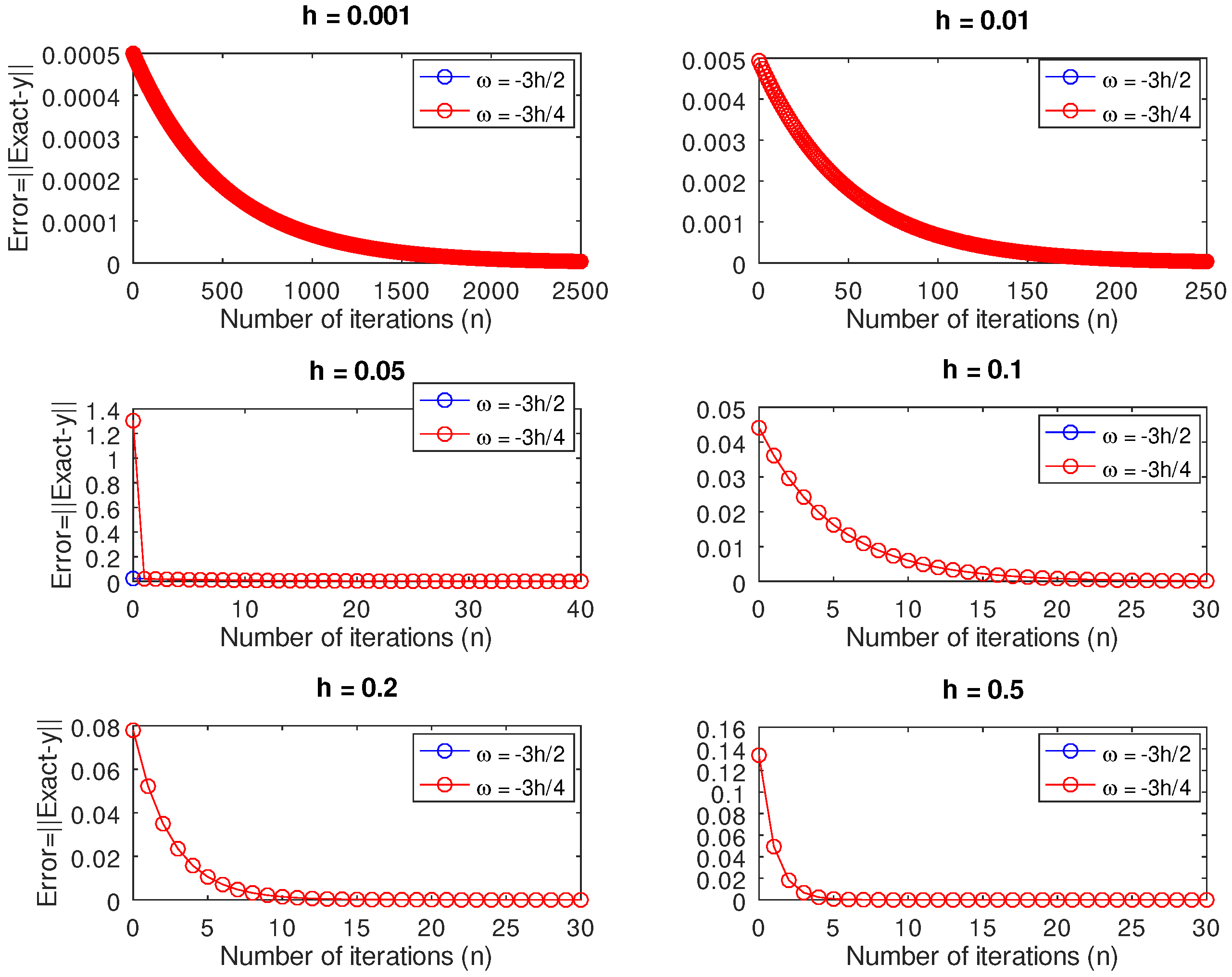
In addition to this, for different values of h, we compared the performance in terms of accuracy to see if there was a huge difference between the approximations obtained for $\omega =-\frac{3h}{4}$ and $\omega =-\frac{3h}{2}$. Since we did not want to compare oranges with apples, we limited our comparison to the norm of the difference between the vector of the exact solution and the vector ${[y_{n+1},y_{n+\frac{3}{2}}]}^T$, albeit they had the same right-hand value (against which only the corresponding entries were compared). In this example, we observed as shown in Figure 3, that for $h=0.001$, while it took $n\ge 2500$ iterations for us to achieve values less than macheps, it took 250 iterations for $h=0.01$, 40 iterations for $h=0.05$ and 30 iterations for $h=0.1,0.2$ and 0.5, respectively. We noticed several overlaps in all values of h considered, as it was very difficult to differentiate between the red and blue lines, signifying no difference in accuracy.

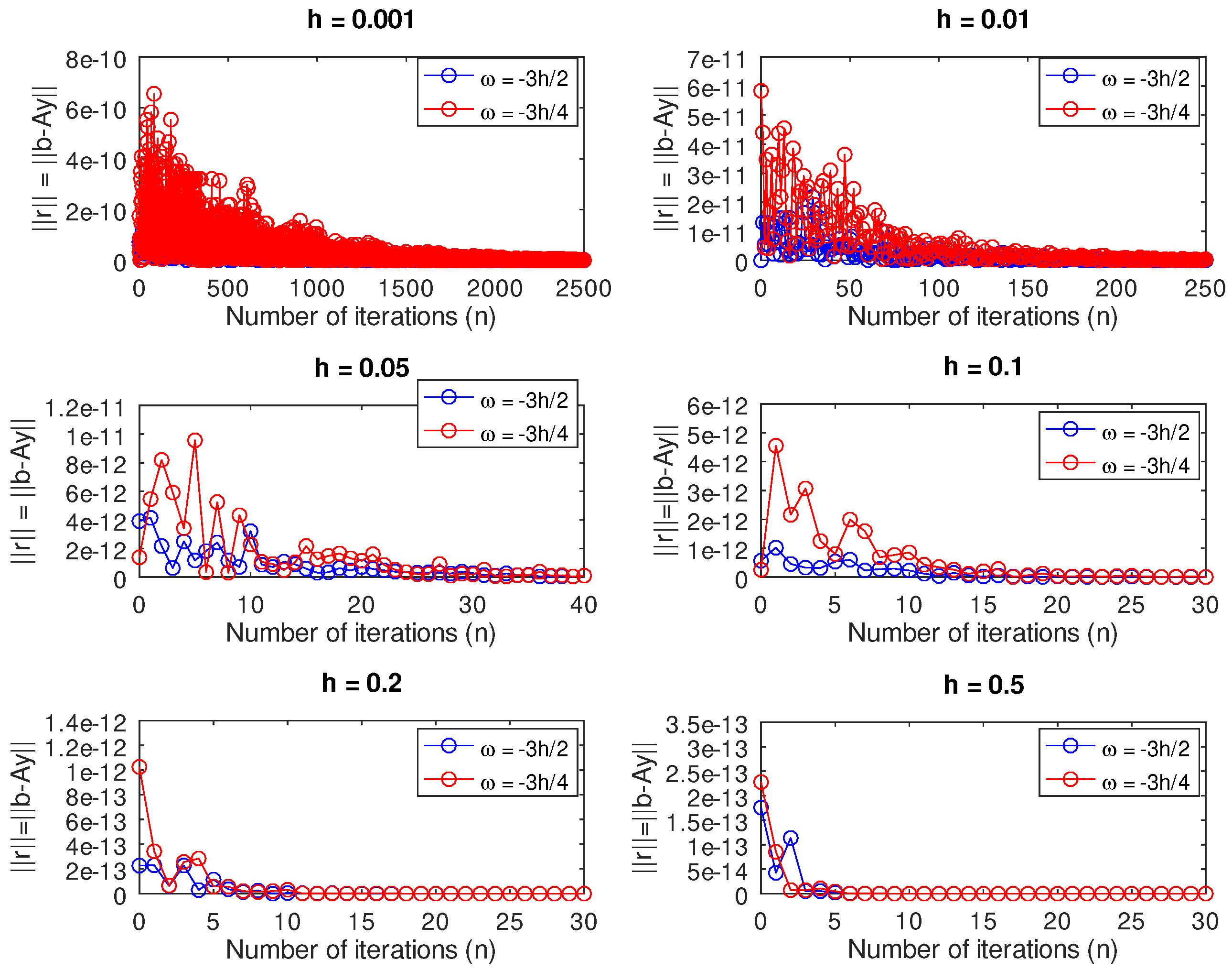
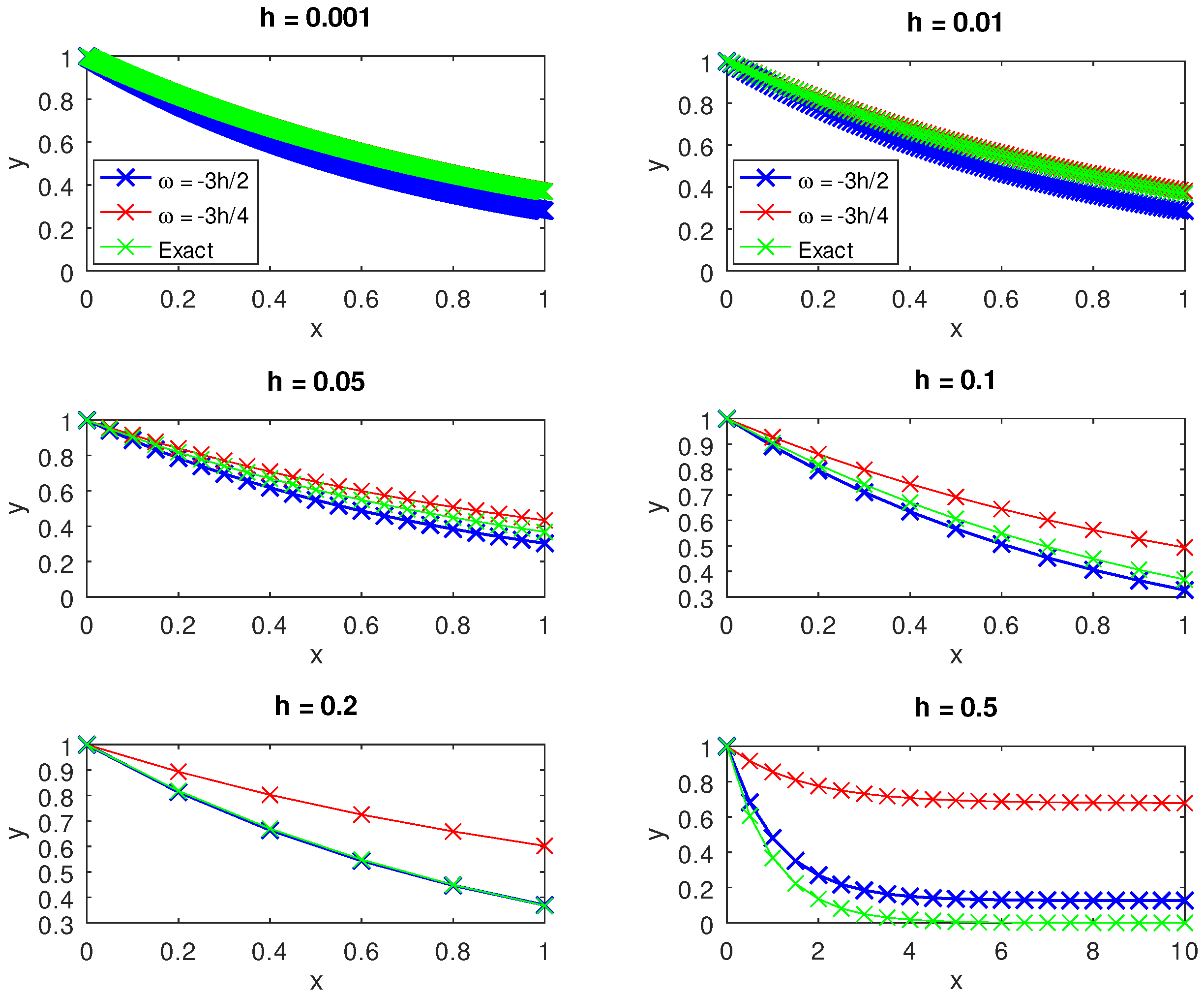
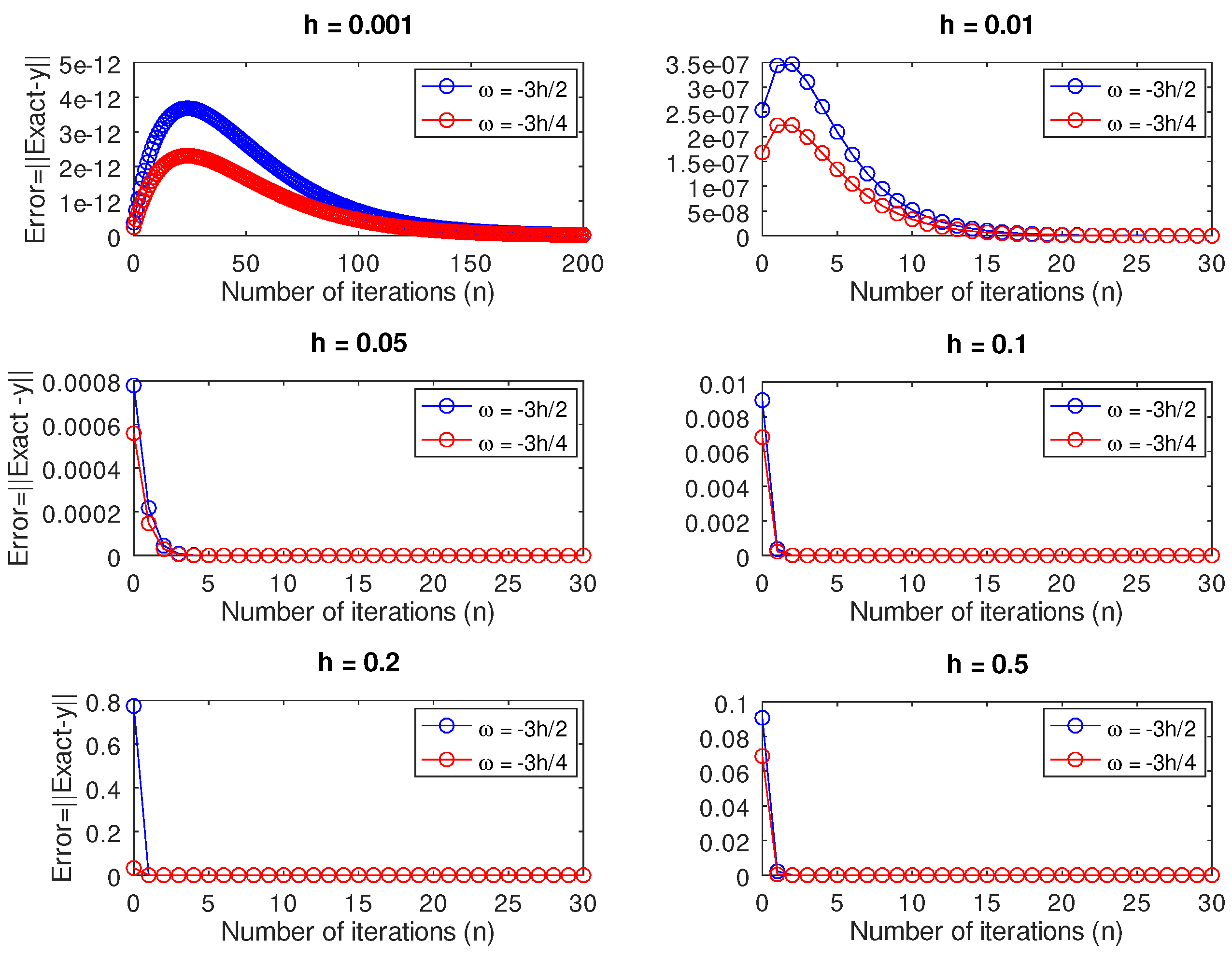
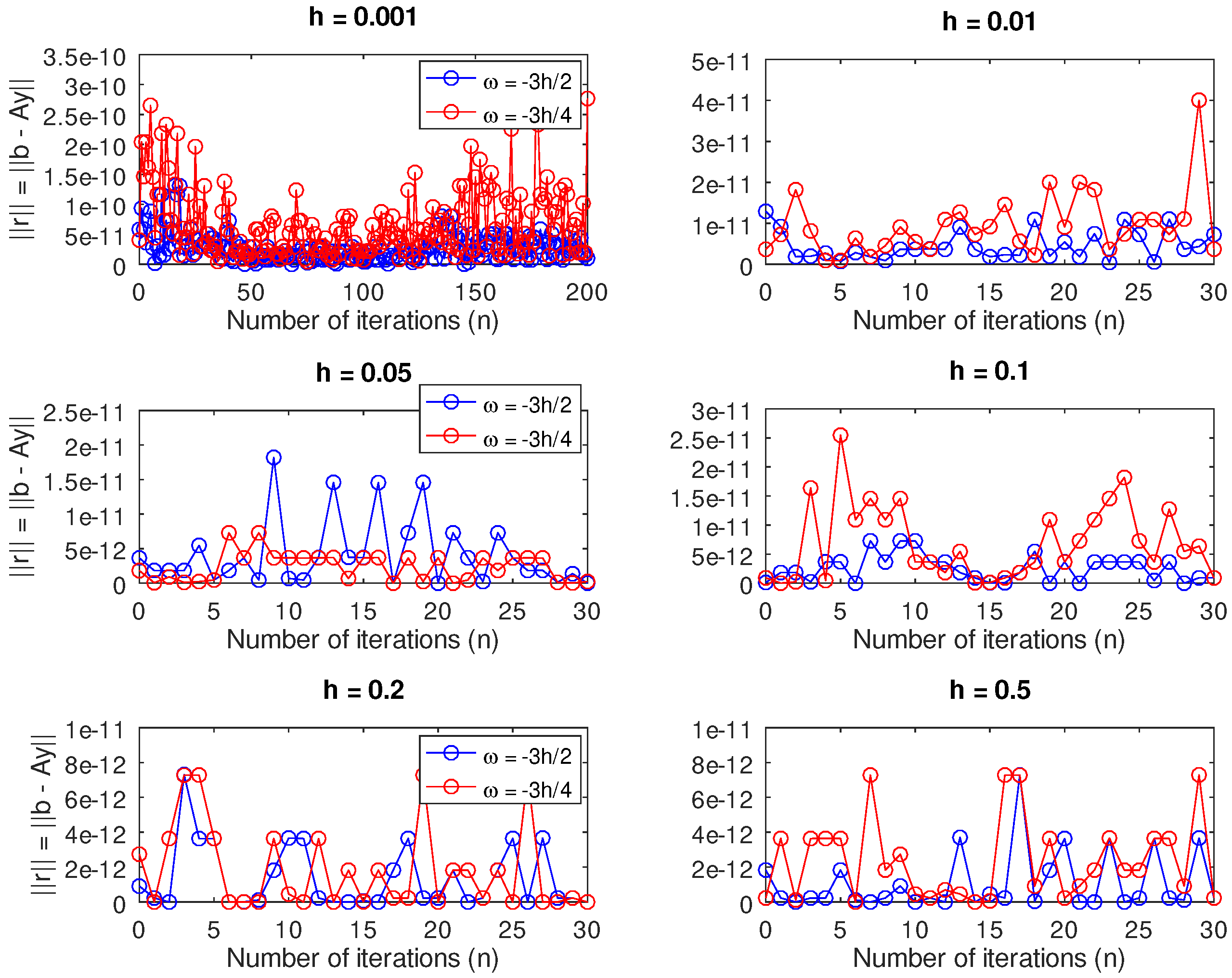
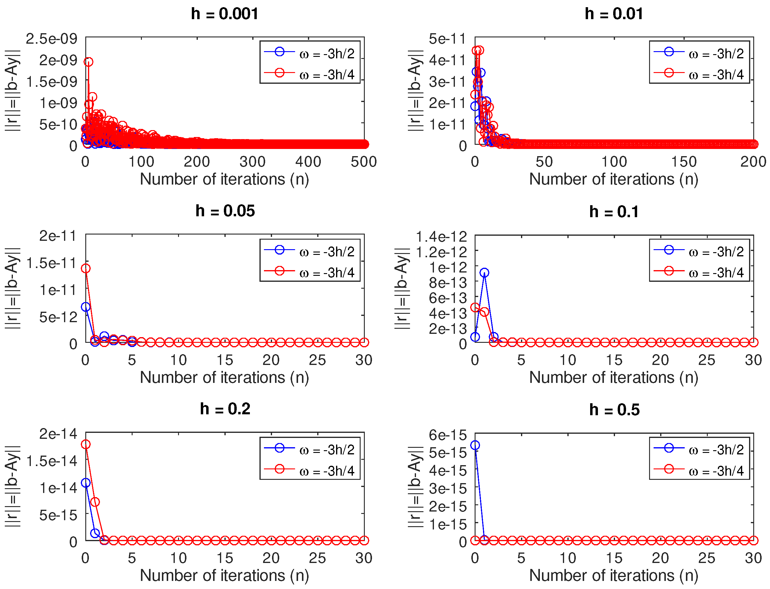
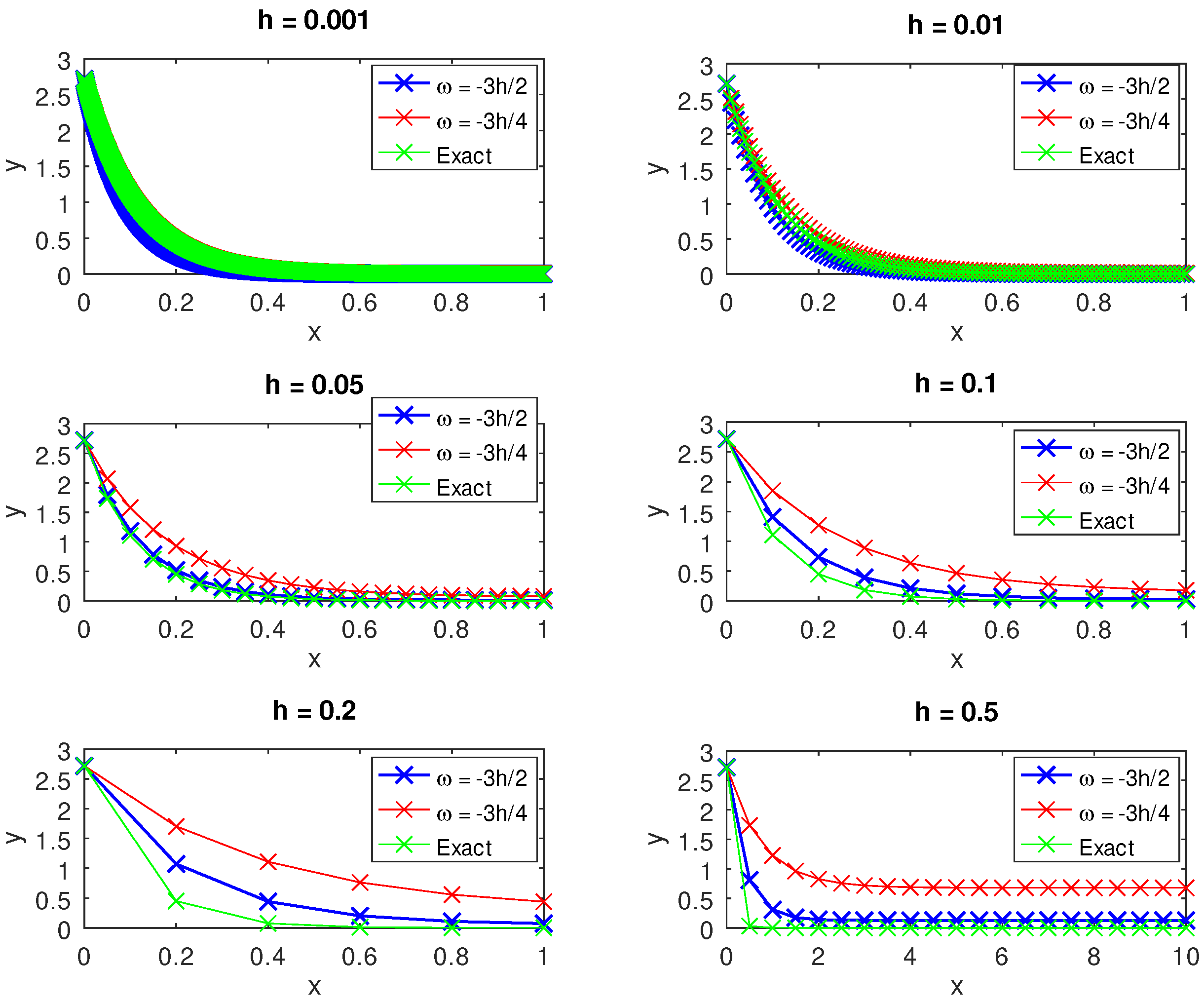
Furthermore, Figure 4 shows a plot of the norm of the residual versus the number of iterations for $\omega =-\frac{3h}{4}$ and $\omega =-\frac{3h}{2}$. We see that the schemes (7)–(10) corresponding to $\omega =-\frac{3h}{2}$, depicted by the blue lines, have a smaller norm of residual compared to the discrete schemes (3)–(10) corresponding to $\omega =-\frac{3h}{4}$, represented by the red lines. Lastly, we solved the underdetermined systems (21) and (22) for different values of h and the results are shown in Figure 5. Initially we observed that for $h=0.001$ and $h=0.01$, there were disparities in the errors between the blue and the red lines. Nevertheless, as the value of h increased, we noticed very good performance for the scheme represented by the blue line compared to the red line for $h=0.05,0.2$ and $h=0.1$. Lastly, we solved the initial value problem using Newton–Raphson’s method as shown in Figure 6, which is self-explanatory and enforces the validity of our work.

Example 2.

We seek the IVP $y^{\prime }=-20y+20sinx+cosx$ with initial condition $y\left(0\right)=y_0=1$ and exact solution $y\left(x\right)=e^{-20x}+sin\left(x\right)$ for $h=0.001,h=0.01,h=0.05,h=0.1,h=0.2$ and $h=0.5$.

Using the discrete schemes (3)–(6) in block form with $y^{\prime }=f(x,y)=-20x+20sinx+cosx$, we multiply both sides of (3) by $\frac{93}{h}$, substitute $n=0$, replace $f_0=f(x_0,y_0)=-y_0$, $f_1=f(x_1,y_1)=-y_1$, $f_{\frac{3}{2}}=f(x_{\frac{3}{2}},y_{\frac{3}{2}})=-y_{\frac{3}{2}}$ and $f_2=f(x_2,y_2)=-y_2$. This yields

$$\begin{array}{cc}\hfill \frac{93}{h}{y}_2& =-\frac{3}{h}{y}_0+\frac{96}{h}{y}_1+[20y_0-20sin{x}_0-cos{x}_0+12(-20y_1+20sin{x}_1+cos{x}_1)\\ & +64(-20y_{\frac{3}{2}}+20sin{x}_{\frac{3}{2}}+cos{x}_{\frac{3}{2}})+15(-20y_2+20sin{x}_2+cos{x}_2)],\end{array}$$

and

$$\begin{array}{c}\hfill \left(240-\frac{96}{h}\right)y_1+1280y_{\frac{3}{2}}+\left(300+\frac{93}{h}\right)y_2=\left(20-\frac{3}{h}\right)y_0+20[12sin{x}_1+64sin{x}_{\frac{3}{2}}\\ \hfill +15sin{x}_2-sin{x}_0]+12cos{x}_1+64cos{x}_{\frac{3}{2}}+15cos{x}_2-cos{x}_0.\end{array}$$

(23)

If we consider (4) and multiply both sides by $\frac{1984}{h}$, then

$$\begin{array}{cc}\hfill \frac{1984}{h}{y}_{\frac{3}{2}}& =\frac{148}{h}{y}_0+\frac{1836}{h}{y}_1+[39(-20y_0+20sin{x}_0+cos{x}_0)+648(-20y_1+20sin{x}_1+cos{x}_1)\\ & +480(-20y_{\frac{3}{2}}+20sin{x}_{\frac{3}{2}}+cos{x}_{\frac{3}{2}})-27(-20y_2+20sin{x}_2+cos{x}_2)],\end{array}$$

and

$$\begin{array}{c}\hfill \left(12960-\frac{1836}{h}\right)y_1+\left(9600+\frac{1984}{h}\right)y_{\frac{3}{2}}-540y_2=\left(\frac{148}{h}-780\right)y_0+20[39sin{x}_0+648sin{x}_1\\ \hfill +480sin{x}_{\frac{3}{2}}-27sin{x}_2]+39cos{x}_0+648cos{x}_1+480cos{x}_{\frac{3}{2}}-27cos{x}_2.\end{array}$$

(24)

In the same vein, after multiplying both sides of (5) by $\frac{31744}{h}$, (6) by $\frac{1984}{h}$ and with some simplifications we obtain, respectively,

$$\begin{array}{c}\hfill \left(152880-\frac{30772}{h}\right)y_1+329280y_{\frac{3}{2}}+\frac{31744}{h}{y}_{\frac{7}{4}}+8820y_2=\left(\frac{972}{h}-4620\right)y_0+20[231sin{x}_0+7644sin{x}_1\\ \hfill +16464sin{x}_{\frac{3}{2}}+441sin{x}_2]+231cos{x}_0+7644cos{x}_1+16464cos{x}_{\frac{3}{2}}+441cos{x}_2.\end{array}$$

(25)

and

$$\begin{array}{c}\hfill \left(-23380-\frac{630}{h}\right)y_1+43120y_{\frac{3}{2}}-39680y_{\frac{7}{4}}+10920y_2=\left(3580-\frac{630}{h}\right)y_0+20[-179sin{x}_0-1169sin{x}_1\\ \hfill +2156sin{x}_{\frac{3}{2}}-1984sin{x}_{\frac{7}{4}}+546sin{x}_2]-179cos{x}_0-1169cos{x}_1+2156cos{x}_{\frac{3}{2}}-1984cos{x}_{\frac{7}{4}}+546cos{x}_2.\end{array}$$

(26)

Since (3) and (4) and (7) and (8) are the same, respectively, there is no need to repeat the steps that led to (23) and (24). Rather, we make the same substitutions as above in (9) and (10) such that

$$\begin{array}{c}\hfill \left(84000+\frac{500}{h}\right)y_1-48000y_{\frac{3}{2}}+\frac{1984}{h}{y}_{\frac{5}{2}}+58500y_2=\left(\frac{2484}{h}-14700\right)y_0+20[735sin{x}_0+4200sin{x}_1\\ \hfill -2400sin{x}_{\frac{3}{2}}+2925sin{x}_2]+735cos{x}_0+4200cos{x}_1-2400cos{x}_{\frac{3}{2}}+2925cos{x}_2.\end{array}$$

(27)

and

$$\begin{array}{c}\hfill \left(27200+\frac{900}{h}\right)y_1-24400y_{\frac{3}{2}}-2480y_{\frac{5}{2}}+12300y_2=\left(\frac{900}{h}-5380\right)y_0+20[269sin{x}_0+1360sin{x}_1\\ \hfill -1220sin{x}_{\frac{3}{2}}-124sin{x}_{\frac{5}{2}}+615sin{x}_2]+269cos{x}_0+1360cos{x}_1-1220cos{x}_{\frac{3}{2}}-124cos{x}_{\frac{5}{2}}+615cos{x}_2.\end{array}$$

(28)

are immediate, respectively. Upon imposing the initial condition $y_0=1$ and substituting $h=0.1,0.2$, etc., appropriately, we obtain the results. Computationally speaking, after computing for $n=0$ outside the for loop, we loop for $n=1,2,\cdots$ by replacing

$$[x_1,x_{\frac{3}{2}},x_2,x_{\frac{5}{2}}],$$

with, respectively,

$$[2n+1,\left(2n+\frac{1}{2}\right),2n,\left(2n+\frac{5}{2}\right)]h,$$

on the one hand and

$$[x_1,x_{\frac{3}{2}},x_{\frac{7}{4}},x_2],$$

with, respectively,

$$[2n+1,\left(2n+\frac{1}{2}\right),\left(2n+\frac{7}{4}\right),2n]h,$$

on the other. The results of the numerical experiments are shown in Table 3 as well as Figure 7, Figure 8, Figure 9 and Figure 10. Table 3 row eight, columns two and three show that for $h=0.5$, we were able to reduce the $\kappa \left(\mathbf{A}\right)$ from 943.79 to 401.77 by changing the grid point from $x_{n+\frac{7}{4}}$ to $x_{n+\frac{5}{2}}$ corresponding to $\omega =-\frac{3h}{4}$ and $\omega =-\frac{3h}{2}$, respectively. In the same vein, by solving an underdetermined system of equations derived from the discrete schemes (11) and (12), we further reduced the condition number from 943.79 to 63.53 corresponding to the grid point $x_{n+\frac{7}{4}}$ ($\omega =-\frac{3h}{4}$) and from 401.77 to 32.39 corresponding to the grid point $x_{n+\frac{5}{2}}$ ($\omega =-\frac{3h}{2}$), respectively. This example also shows that with a carefully chosen grid point, one can successfully avoid solving an ill-conditioned linear system of equations.

Table 3. Comparison of the condition numbers for the matrices derived from Example 3.

	$\mathit{\kappa }\left(\mathbf{A}\right)$	$\mathit{\kappa }\left(\mathbf{B}\right)$	$\mathit{\kappa }\left(\mathbf{C}\right)$	$\mathit{\kappa }\left(\mathbf{E}\right)$
$\mathit{h}$	$\mathbf{\omega }=-\frac{\mathbf{3}\mathit{h}}{\mathbf{4}}$	$\mathbf{\omega }=-\frac{\mathbf{3}\mathit{h}}{\mathbf{2}}$	$\mathbf{\omega }=-\frac{\mathbf{3}\mathit{h}}{\mathbf{4}}$	$\mathbf{\omega }=-\frac{\mathbf{3}\mathit{h}}{\mathbf{2}}$
Size of matrix	$4\times 4$	$4\times 4$	$2\times 4$	$2\times 4$
0.001	484.04	30.45	7.09	9.84
0.010	504.68	30.61	8.55	10.43
0.050	540.51	42.62	16.84	14.29
0.100	523.26	68.44	28.35	19.30
0.200	494.89	120.17	46.31	26.15
0.500	636.20	259.00	62.22	31.70

Figure 7. Comparison of the norm of the difference between the exact solution and the vector ${[y_{n+1},y_{n+\frac{3}{2}}]}^T$ for different values of h using the discrete schemes (3)–(6) corresponding to $\omega =-\frac{3h}{4}$ and the discrete schemes (7)–(10) corresponding to $\omega =-\frac{3h}{2}$.

Figure 8. Comparison of the norm of the residual for different values of h using the discrete schemes (3)–(6) corresponding to $\omega =-\frac{3h}{4}$ and the discrete schemes (7)–(10) corresponding to $\omega =-\frac{3h}{2}$.

Figure 9. Comparison of the norm of the difference between the exact solution and the vector ${[y_{n+1},y_{n+2}]}^T$ for different values of step sizes using the discrete schemes (11) corresponding to $\omega =-\frac{3h}{4}$ and the discrete schemes (12) corresponding to $\omega =-\frac{3h}{2}$, by solving an underdetermined system of linear equations.

Figure 10. Comparison of the exact solution with those obtained from the discrete scheme (6) corresponding to $\omega =-\frac{3h}{4}$ and the discrete scheme (10) corresponding to $\omega =-\frac{3h}{2}$, using Newton’s method.

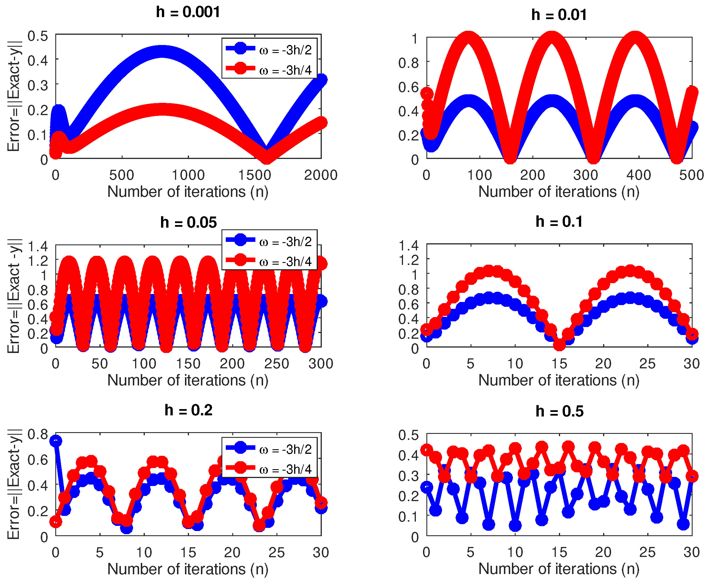
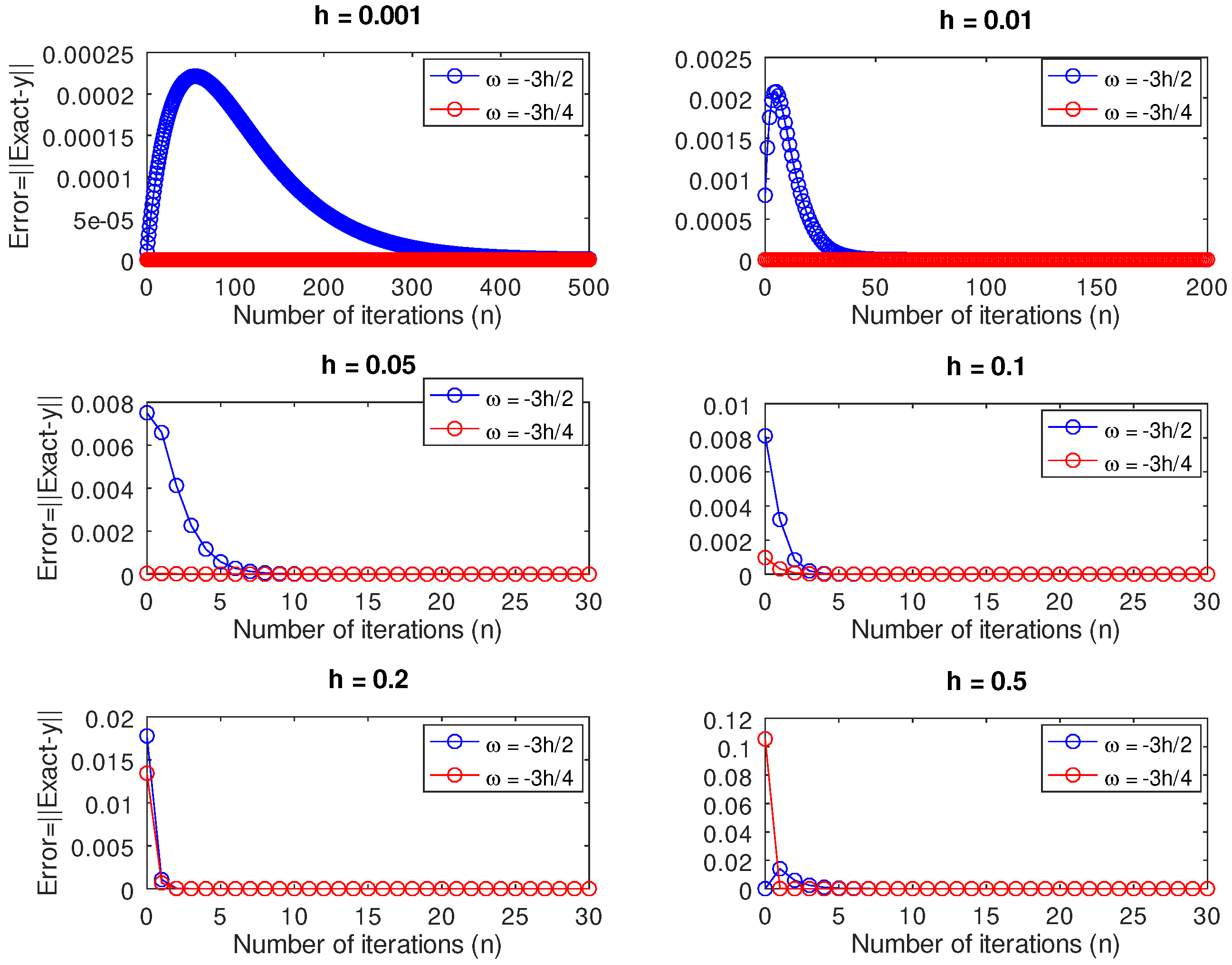
As shown in Figure 7, we see that although there were initial disparities in the plot of the error against the number of iterations for $h=0.001$ and $h=0.01$, as n increased, this difference fizzled out and for the remaining values of h, we observe that there was hardly any noticeable difference between the accuracy of the two schemes in the absence of round-off errors. With the exception of $h=0.05$, Figure 8 shows that the performance of the accuracy at the two grid points is the same. As shown in Figure 9, with the exception of $h=0.001$, the error obtained by solving the underdetermined linear system of equations using $\omega =-\frac{3h}{2}$ was much smaller than that from using $\omega =-\frac{3h}{4}$ in the remaining step sizes. Using Newton’s method and as shown in Figure 9, we see that the new scheme corresponding to $\omega =-\frac{3h}{2}$ performed better in terms of accuracy than the scheme corresponding to $\omega =-\frac{3h}{4}$ for $h=0.2$ and $0.5$. We used the one-dimensional Newton–Raphson method to solve the same example and Figure 10 shows results of the numerical experiment that the error was smaller for $\omega =-\frac{3h}{2}$ than $\omega =-\frac{3h}{4}$.

Example 3.

We seek numerical approximations to the initial value problem $y^{\prime }=-9y$ with initial condition $y\left(0\right)=e$, for $h=0.001,h=0.01,h=0.05,h=0.1,h=0.2,h=0.5$ with $y\left(x\right)=e^{1-9x}$ as an exact solution.

We substituted $f(x,y)=-9y$ into each of the discrete schemes (3)–(6), (7)–(10), (11) and (12) for $h=0.001,h=0.01,h=0.05,h=0.1,h=0.2,h=0.5$ and n. The results of the numerical experiments are shown in Table 4 as well as Figure 11, Figure 12, Figure 13 and Figure 14. Table 4 row seven, columns two and three show that for $h=0.2$, we were able to reduce the $\kappa \left(\mathbf{A}\right)$ from 494.89 to 120.17 by changing the grid point from $x_{n+\frac{7}{4}}$ to $x_{n+\frac{5}{2}}$ corresponding to $\omega =-\frac{3h}{4}$ and $\omega =-\frac{3h}{2}$, respectively. In the same vein, by solving an underdetermined system of equations derived from the discrete schemes (11) and (12), we further reduced the condition number from 494.89 to 46.21 corresponding to the grid point $x_{n+\frac{7}{4}}$ ($\omega =-\frac{3h}{4}$) and from 120.17 to 26.15 corresponding to the grid point $x_{n+\frac{5}{2}}$ ($\omega =-\frac{3h}{2}$), respectively. This example also shows that with a carefully chosen grid point, one can successfully avoid solving an ill-conditioned linear system of equations.

Table 4. Comparison of the condition numbers for the matrices derived from Example 2.

	$\mathit{\kappa }\left(\mathbf{A}\right)$	$\mathit{\kappa }\left(\mathbf{B}\right)$	$\mathit{\kappa }\left(\mathbf{C}\right)$	$\mathit{\kappa }\left(\mathbf{E}\right)$
$\mathit{h}$	$\mathbf{\omega }=-\frac{\mathbf{3}\mathit{h}}{\mathbf{4}}$	$\mathbf{\omega }=-\frac{\mathbf{3}\mathit{h}}{\mathbf{2}}$	$\mathbf{\omega }=-\frac{\mathbf{3}\mathit{h}}{\mathbf{4}}$	$\mathbf{\omega }=-\frac{\mathbf{3}\mathit{h}}{\mathbf{2}}$
Size of matrix	$4\times 4$	$4\times 4$	$2\times 4$	$2\times 4$
0.001	487.14	30.36	7.28	9.91
0.010	524.45	32.41	10.78	11.48
0.050	517.65	71.35	30.77	20.29
0.100	496.70	132.23	49.06	27.11
0.200	601.39	237.34	61.31	31.35
0.500	943.79	401.77	63.53	32.39

Figure 11. Comparison of the norm of the difference between the exact solution and the vector ${[y_{n+1},y_{n+2}]}^T$ for different values of step sizes using the discrete schemes (11) corresponding to $\omega =-\frac{3h}{4}$ and the discrete schemes (12) corresponding to $\omega =-\frac{3h}{2}$, by solving an underdetermined system of linear equations.

Figure 12. Comparison of the norm of the difference between the exact solution and the vector ${[y_{n+1},y_{n+\frac{3}{2}}]}^T$ for different values of h using the discrete schemes (3)–(6) corresponding to $\omega =-\frac{3h}{4}$ and the discrete schemes (7)–(10) corresponding to $\omega =-\frac{3h}{2}$.

Figure 13. Comparison of the norm of the residual for different values of step sizes using the discrete schemes (3)–(6) corresponding to $\omega =-\frac{3h}{4}$ and the discrete schemes (7)–(10) corresponding to $\omega =-\frac{3h}{2}$.

Figure 14. Comparison of the exact solution with those obtained from the discrete scheme (6) corresponding to $\omega =-\frac{3h}{4}$ and the discrete scheme (10) corresponding to $\omega =-\frac{3h}{2}$, using Newton’s method.

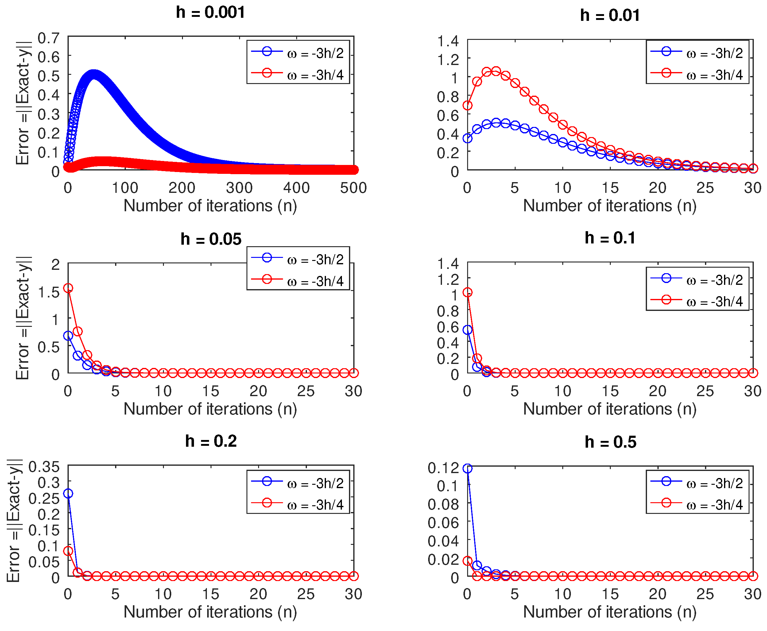
Initially, Figure 12 shows that for $h=0.001$ and $h=0.01$, there was a slow convergence to the exact solution by evaluating at the grid point $x_{n+\frac{5}{2}}$ compared to $x_{n+\frac{7}{4}}$. These two step sizes corresponded to the two instances in which the $\mathbf{D}$ matrix was singular. A similar scenario pans out for $h=0.05$ and $h=0.1$, in which cases the matrix $\mathbf{D}$ was nearly singular but the convergence was quicker than that of the former choices of h. We obtained better approximations to the exact solution for those two values of h in which the $\mathbf{D}$ matrix was nonsingular. However, we noticed in Figure 13 that there were no significant differences between the norm of the residual of the two schemes. Except when $h=0.001$, Figure 11 shows that by solving the resulting underdetermined system of equations using the two schemes (11) and (12), the error is smaller in the remaining step sizes for $\omega =-\frac{3h}{2}$ than for $\omega =-\frac{3h}{4}$.

5. Conclusions

The aim of this paper was achieved, in the sense that we reduced the condition number of the linear systems of equations derived from initial value problems with a carefully chosen grid point $x=x_{n+\frac{5}{2}}$ corresponding to $\omega =-\frac{3h}{2}$ instead of $x=x_{n+\frac{7}{4}}$ corresponding to $\omega =-\frac{3h}{4}$. In addition, we discovered that the order of the discrete scheme was preserved with this choice but with a different error constant. Henceforth, we suggest that researchers should pay rapt attention to the choice of the grid point so as to avoid solving ill-conditioned systems. We also showed that this condition number could be further reduced if one solves an underdetermined system of two equations in four unknowns for both stiff and nonstiff initial value problems. When compared with the exact solution, the results of numerical experiments showed that the new scheme outperformed the former.

References

- Shampine, L.F. Ill-conditioned matrices and the integration of stiff ODEs. J. Comput. Appl. Math. 1993, 48, 279–292. [Google Scholar] [CrossRef]
- Akinola, R.O.; Ajibade, K.J. A Proof of the Non-Singularity of the D Matrix Used in Deriving the two–Step Butcher’s Hybrid Scheme for the Solution of Initial Value Problems. J. Appl. Math. Phys. 2021, 9, 3177–3201. [Google Scholar] [CrossRef]
- Burden, R.L.; Faires, J.D. Numerical Analysis, 9th ed.; Richard Stratton: Boston, MA, USA, 2011. [Google Scholar]
- Ortega, J.M. Numerical Analysis; A Second Course; Academic Press: New York, NY, USA, 1972; Volume 201, p. 33. [Google Scholar]
- Golub, G.H.; Wilkinson, J.H. Ill-conditioned eigensystems and the computation of the Jordan canonical form. SIAM Rev. 1976, 18, 578–619. [Google Scholar] [CrossRef]
- Peters, G.; Wilkinson, J.H. Inverse iteration, ill-conditioned equations and Newton’s method. SIAM Rev. 1979, 21, 339–360. [Google Scholar] [CrossRef]
- Farooq, M.; Salhi, A. Improving the solvability of Ill–conditioned systems of linear equations by reducing the condition number of their matrices. J. Korean Math. Soc. 2011, 48, 939–952. [Google Scholar] [CrossRef]
- Douglas, C.C.; Lee, L.; Yeung, M. On Solving Ill Conditioned Linear Systems. Procedia Comput. Sci. 2016, 80, 941–950. [Google Scholar] [CrossRef]
- Sirisina, U.W.; Kumleng, G.M.; Yahaya, Y.A. A New Butcher Type two-Step Block Hybrid Multistep Method for Accurate and Efficient Parallel Solution of Ordinary Differential Equations. Abacus Math. Ser. 2004, 31, 1–7. [Google Scholar]
- Akinola, R.O. An Accurate Implementation of the Two-Step Butcher’s Hybrid Scheme on Initial Value Problems. Bachelor’s Thesis, University of Jos, Jos, Nigeria, 2001. [Google Scholar]
- Demmel, J.W. Applied Numerical Linear Algebra; Society for Industrial and Applied Mathematics: Philadelphia, PA, USA, 1997. [Google Scholar]
- Chen, W.; Wu, W.X.; Teng, Z.D. Complete Dynamics in a Nonlocal Dispersal Two-Strain SIV Epidemic Model with Vaccinations and Latent Delays. Appl. Comput. Math. 2020, 19, 360–391. [Google Scholar]
- Kamoh, N.M.; Gyemang, D.G.; Soomiyol, M.C. On One Justification on the Use of Hybrids for the Solution of First Order Initial Value Problems of Ordinary Differential Equations. Pure Appl. Math. J. 2017, 6, 137–143. [Google Scholar]
- Adiguzel, R.S.; Aksoy, U.; Karapinar, E.; Erhan, I.M. On the solutions of Fractional Differential Equations via Geraghty Type Hybrid Contractions. Appl. Comput. Math. 2021, 20, 313–333. [Google Scholar]
- Adee, S.O.; Atabo, V.O. Improved two-Point Block Backward Differentiation Formulae for Solving First Order Stiff Initial Value Problems of Ordinary Differential Equations. Niger. Ann. Pure Appl. Sci. 2020, 3, 200–209. [Google Scholar] [CrossRef]
- Ozyapici, A.; Karanfiller, T. New integral operator for solutions of differential equations. TWMS J. Pure Appl. Math. 2020, 11, 131–143. [Google Scholar]
- Shokri, A. The symmetric P-stable Hybrid Obrenchkoff Methods for the numerical solution of second order IVPs. TWMS J. Pure Appl. Math. 2012, 5, 28–35. [Google Scholar]
- Shokri, A. An explicit trigonometrically fitted ten-step method with phase-lag of order infinity for the numerical solution of the radial Schrodinger equation. J. Appl. Comput. Math. 2015, 14, 63–74. [Google Scholar]
- Shokri, A.; Tahmourasi, M. A new two-step Obrenchkoff method with vanished phase-lag and some of its derivatives for the numerical solution of radial Schrodinger equation and related IVPs with oscillating solutions. Iran. J. Math. Chem. 2017, 8, 137–159. [Google Scholar]
- Sunday, J.; Chigozie, C.; Omole, E.O. A pair of three-step hybrid block methods for the solutions of linear and non-linear first order systems. Eur. J. Math. Stat. 2022, 3, 13–23. [Google Scholar] [CrossRef]
- Omole, E.O.; Jeremiah, O.A.; Adoghe, L.O.A. A class of Continuous Implicit Seventh–eight method for solving y′=f(x,y) using power series. Int. J. Chem. Math. Phys. 2020, 4, 39–50. [Google Scholar] [CrossRef]
- Mohammed, U.; Adeniyi, R.B. A Three Step Implicit Hybrid Linear Multistep Method for the Solution of Third Order Ordinary Differential Equations. Gen. Math. Notes 2014, 25, 62–74. [Google Scholar]
- Mohammed, U.; Jiya, M.; Mohammed, A.A. A class of six step block method for solution of general second order ordinary differential equations. Pac. J. Sci. Technol. 2010, 11, 273–277. [Google Scholar]
- Mohammed, U. A class of implicit five step block method for general second order ordinary differential equations. J. Niger. Math. Soc. 2010, 30, 25–39. [Google Scholar]
- Awoyemi, D.O. A P-stable linear multistep method for solving general third order of ordinary differential equations. Int. J. Comput. Math. 2003, 80, 985–991. [Google Scholar] [CrossRef]
- Awoyemi, D.O.; Idowu, O. A class hybrid collocation methods for third order of ordinary differential equations. Int. J. Comput. Math. 2005, 82, 1287–1293. [Google Scholar] [CrossRef]
- Awoyemi, D.O.; Kayode, S.J.; Adoghe, L.O. A four–point fully implicit method for numerical integration of third-order ordinary differential equations. Int. J. Phys. Sc. 2014, 9, 7–12. [Google Scholar] [CrossRef]
- Sagir, A.M. On the approximate solution of continuous coefficients for solving third order ordinary differential equations. Int. J. Math. Comput. Sci. Eng. 2014, 8, 39–43. [Google Scholar]
- Badmus, A.M.; Yahaya, Y.A. Some multi derivative hybrid block methods for solution of general third order ordinary differential equations. Niger. J. Sci. Res. 2009, 8, 103–107. [Google Scholar]
- Aliev, F.A.; Aliyev, N.A.; Hajiyeva, N.S.; Mahmudov, N.I. Some Mathematical Problems and their solutions for the oscillating systems with Liquid Dampers: A Review. Appl. Comput. Math. 2021, 20, 339–365. [Google Scholar]
- Fatunla, S.O. A class of block methods for second order IVPs. Int. J. Comput. Math. 1994, 55, 119–133. [Google Scholar] [CrossRef]
- Bouazza, Z.; Souid, M.S.; Günerhan, H. Multiterm boundary value problem of Caputo fractional differential equations of variable order. Adv. Differ. Equ. 2021, 2021, 400. [Google Scholar] [CrossRef]
- Hossen, B.; Roshid1, H.; Ali, Z. Modified Double Sub-equation Method for Finding Complexiton Solutions to the (1 + 1) Dimensional Nonlinear Evolution Equations. Int. J. Appl. Comput. Math. 2017, 3, 679–697. [Google Scholar] [CrossRef]
- Adee, S.O.; Onumanyi, P.; Sirisena, U.W.W.; Yahaya, Y.A. Note on starting numerov method more accurately by a hybrid formula of order four for an initial value problem. J. Comput. Appl. Math. 2005, 175, 369–373. [Google Scholar]
- Jator, S.N. A sixth order linear multistep method for the direct solution of y′′′=f(x,y,y′). Int. J. Pure Appl. Math. 2007, 40, 457–472. [Google Scholar]
- Jator, S.N. On the numerical integration of third order boundary value problems by a linear multistep method. Int. J. Pure Appl. Math. 2008, 46, 375–388. [Google Scholar]
- Jator, S.N.; Li, J. A self-starting linear multistep method for a direct solution of the general second order initial value problem. Int. J. Comput. Math. 2007, 86, 827–836. [Google Scholar] [CrossRef]
- Jator, S.N. Multiple finite difference methods for solving third order ordinary differential equations. Int. J. Pure Appl. Math. 2008, 43, 253–265. [Google Scholar]
- Olabode, B.T.; Yusuph, Y. A new block method for special third order ordinary differential equations. J. Math. Stat. 2009, 5, 167–170. [Google Scholar] [CrossRef][Green Version]
- Yahaya, Y.A.; Adegboye, Z.A. Construction and Implementation of a 4-Step Implicit Collocation Method for Solution of First and Second Order ODEs. Pac. J. Sci. Technol. 2012, 13, 159–165. [Google Scholar]
- Henrici, P. Discrete Variable Methods in Ordinary Differential Equations; John Wiley: New York, NY, USA, 1962; p. 407. [Google Scholar]
- Trefethen, L.N.; Bau, D., III. Numerical Linear Algebra; SIAM: Philadelphia, PA, USA, 1997. [Google Scholar]
Publisher’s Note: MDPI stays neutral with regard to jurisdictional claims in published maps and institutional affiliations. |
© 2022 by the authors. Licensee MDPI, Basel, Switzerland. This article is an open access article distributed under the terms and conditions of the Creative Commons Attribution (CC BY) license (https://creativecommons.org/licenses/by/4.0/).