Balancing Cost and Demand in Electricity Access Projects: Case Studies in Ecuador, Mexico and Peru

Abstract

Rural areas in developing countries have the highest concentrations of unelectrified communities. There is a clear link between electricity consumption and the Human Development Index, as highlighted by the 7th Development Goal of the United Nations. Estimating the energy needs of the previously nonelectrified population is imprecise when designing rural electrification projects. Indeed, daily energy demand and peak power assessments are complex, since these values must be valid over the project’s lifetime, while tight budgets do not allow for the systems to be oversized. In order to assist project promoters, this study proposes a fuzzy mixed integer linear programming model (FMILP) for the design of wind–PV rural electrification systems including uncertainty in the demand requirements. Two different FMILP approaches were developed that maximized the minimum or the average satisfaction of the users. Next, the FMILP approaches were applied to six Latin American communities from three countries. Compared with the deterministic MILP (where the energy and peak power needs are considered as specific values), the FMILP results achieved a better balance between the project cost and the users’ satisfaction regarding the energy and peak power supplied. Regarding the two approaches, maximizing the users’ minimum satisfaction obtained globally better solutions.

1. Introduction

“Ensuring access to affordable, reliable, sustainable and modern energy for all” has been recognized as the 7th Sustainable Development Goal of the United Nations [1]. Indeed, a connection exists between the Human Development Index (HDI) and energy access [2]: for less developed regions, slight increases in electricity consumption lead to huge socioeconomic growth, significantly improving the population’s living standards. However, a significant proportion of the population in rural areas of developing countries still lack such a service [3].

Extending electricity access through the national grid can have important techno-economic limitations in rural and remote areas because of the dispersion of demand and low end-user consumption. In contrast, standalone systems based on renewable energy are appropriate for isolated communities [4]. In particular, hybrid wind–photovoltaic (PV) systems can reduce costs and improve supply quality in comparison with single-technology projects [5]. Hybrid systems have proven to be suitable to address the electricity needs of residential clusters [6]. Additionally, the combination of individual supplies and microgrids can help medium-dispersed communities achieve a proper balance between extension lines and cost increases [7]. However, the whole design is complex, having to study many locations and sizes for generators, along with all possible connections among demand points to form the corresponding microgrids [8]. Hence, decision support tools are recommended for designing electrification systems correctly [8,9].

There is ample literature dealing with design tools for rural electrification systems including mathematical models and heuristic algorithms [10,11,12]. Many works focus on dimensioning a combination of generation technologies to cover the demand at minimum cost. The most used software is HOMER [13], which includes a detailed analysis of the demand, the energy resources and the equipment. For instance, Raji and Luta [14] used HOMER to design a community microgrid in South Africa, obtaining a technically and economically viable solution. Other optimization methods, such as integer linear programming, have also been used to evaluate wind–PV systems [15]. On the other hand, the distribution of electricity from generators to end users has been less studied [16], with the particular context of medium-dispersed communities receiving even less attention. ViPOR [17] considers, through simulated annealing, the location and electricity needs of each demand point to evaluate whether microgrid extension or individual supply is less expensive. García-Villoria et al. [18] developed a heuristic process to find the minimum cost combination of wind and PV technologies as well as microgrids and individual systems to distribute electricity in remote and medium-dispersed communities.

In the above works, demand was considered as a deterministic value, and the results are, therefore, subject to the quality of its estimation [19]. Consequently, the estimation of demand becomes critical, since an underestimation can leave the inhabitants dissatisfied, while an overestimation can unnecessarily increase the project costs. Inexact predictions will negatively impact the socioeconomic development of the area and/or produce economically unsustainable solutions. However, the real demand can be influenced by several factors such as [11] the local climate and geographic characteristics, the economy and culture, or the typology of consumers and their lifestyle. Therefore, the estimation of demand is inevitably subject to uncertainty [20,21].

In order to obtain robust designs regarding demand uncertainty, different approaches have been developed [22]. A relevant research area has focused on developing predictive algorithms for future demand estimation. For instance, genetic algorithms have been used to forecast the electricity requirements of populations in Turkey [23], Iran [24] and Mauritius [25]. For this purpose, social, economic and environmental indicators are gathered, and optimization algorithms aim to minimize deviation indicators. These algorithms have also been combined with artificial neural networks to improve the prediction results [26]. Under a different approach, Domenech et al. [27] developed an optimization–multicriteria methodology to design wind–PV electrification projects, which, first, generates a set of solutions for different demand scenarios and then selects the best one in terms of several criteria. Nevertheless, the project promoter still has to quantify the demand scenarios as unique values. From a different perspective, fuzzy logic can help solve complex problems with data uncertainty in the energy sector [28]. For instance, Onar et al. [29] developed a decision model with multiple fuzzy criteria for different experts to aid investors in selecting the most appropriate energy technology. Li et al. [30] proposed a fuzzy programming approach for planning an electrical energy generating system. Mohammadi et al. [31] introduced fuzzy elements in an MILP model to help in planning energy systems managing demand uncertainty. The results can help to achieve a balance between the guaranteed energy, the system cost and environmental problems. Vahedipour-Dahraie et al. [32] proposed a risk-averse probabilistic framework to schedule virtual power plants, taking into account demand response and uncertainty. The model helps to mitigate the negative impacts of uncertainty on the plant’s performance. Wang et al. [33] developed a stochastic multiobjective model to design hybrid energy systems, considering demand and solar radiation uncertainty through probability distributions.

The reviewed works focused mainly on large- or medium-sized energy systems, while the analysis of demand uncertainty in the context of small-scale systems for newly electrified populations is scarce (Hossain et al.) [34]. As indicated by Domenech et al. [8], ad hoc tools considering the specific details of end users are required in order to improve the medium- and long-term sustainability of energy systems for these populations. Galleguillos-Pozo et al. [35] developed and compared five fuzzy MILP (FMILP) models, considering different assumptions, to design PV systems that balance the project cost and the demand satisfaction. This paper combined wind energy, controllers and batteries as well as detailed novel electrical features to make the most efficient FMILP model for exploring a wider range of solutions and obtaining better and more detailed electrification options. Hence, two FMILP models are proposed for designing wind–PV rural electrification projects, defining the best location and size of equipment for distribution through microgrids and individual supplies.

Consequently, the project promoters obtained a very powerful tool to assist in decision making when implementing projects in developing countries as well as robust solutions that are not dependent on the exact estimation of demand. Two modeling assumptions were considered and compared for the FMILP model: (a) to ensure that the least satisfied user was as satisfied as possible; (b) to ensure that the global satisfaction of all users was as high as possible. To validate the proposed solution procedure, six case studies were solved: six real communities from three Latin American countries (i.e., Ecuador, Mexico and Peru). The characteristics of the regions studied vary significantly (i.e., forest, semi-arid and highland), which tested the model’s performance in different contexts. The solutions obtained (with FMILP) were compared with those that would have been obtained without considering demand uncertainty (with MILP). Compared to MILP, the FMILP results achieved a better balance between the project cost and the users’ satisfaction in terms of the energy and peak power supplied. Regarding the modeling approaches, maximizing the minimum satisfaction obtained globally better solutions.

The remainder of the paper is organized as follows: Section 2 describes the specific problem including the design of wind–PV systems and uncertainty in users’ demand estimation; Section 3 details the FMILP models for balancing the cost and the demand supplied; Section 4 presents the six case studies and the input data for the validation; Section 5 discusses the results of the case studies; finally, Section 6 highlights the main conclusions.

2. Problem Description

This section first describes the technical considerations of PV–wind electrification systems (Section 2.1); then, the complexity of estimating the electricity demand of end users is highlighted (Section 2.2).

2.1. Systems Design

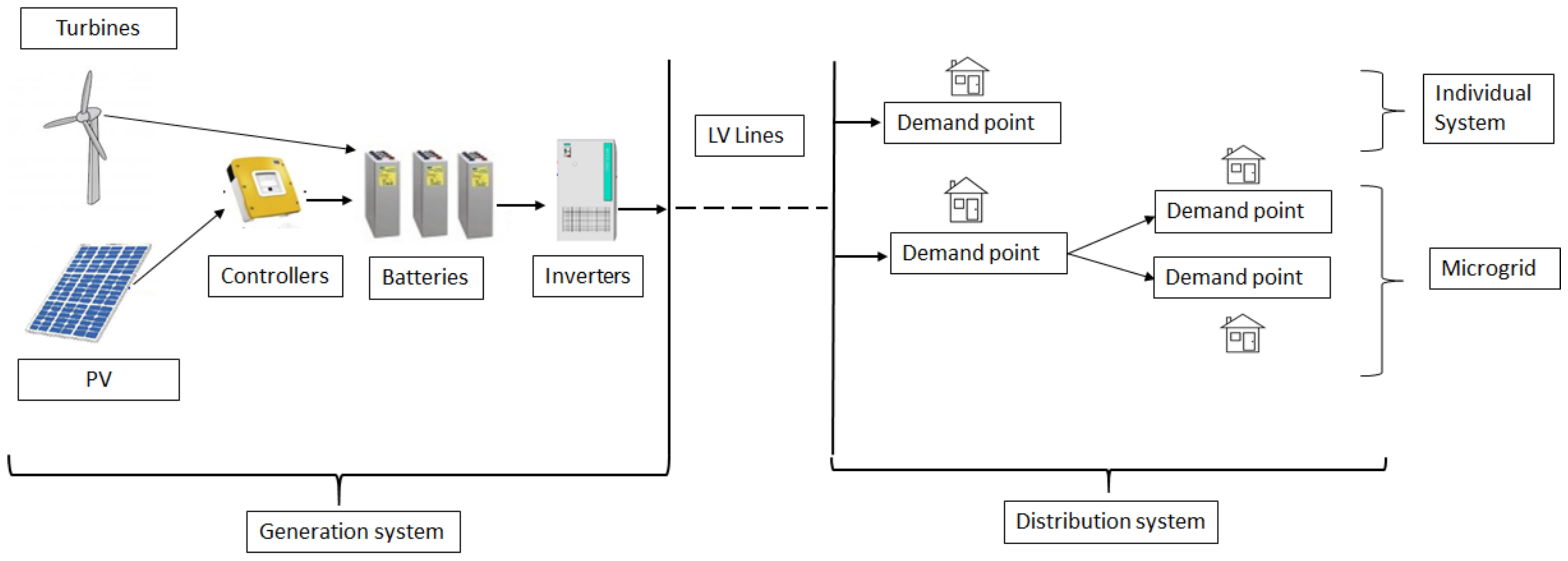
Figure 1 shows the elements of the electrification systems dealt with in this paper (adapted from [36]). The population was dispersed among the demand points (houses, schools, health centers, etc.), each at a different location and having its own energy and peak power requirements. PV panels and wind turbines were used in order to supply the demand. Controllers protected the charge and discharge of the batteries, where the energy was stored for supply during non-generation periods. Next, inverters transformed the DC from the batteries into AC, which is better suited for most appliances. All this equipment was placed at a generation point, which was the only demand point in the case of individual systems or one of the demand points in the case of microgrids. The electricity was distributed at low voltage (LV) among microgrid demand points, using a radial structure suitable for rural areas in developing countries [17]. In addition, meters were installed at microgrid points to track users’ consumption.

Figure 1. Scheme of the rural electrification systems (adapted from [36]).

2.2. Demand Estimation

Determining the energy and peak power demand of end users is complex and involves quantitative and qualitative information regarding the population as well as the energy sources prior to electrification [20]. In order to gather such information, local and regional databases can be consulted, end-users surveyed and interviewed and meetings held with specific categories of the population (women, children, elders, etc.). In addition, the surroundings of the community must be examined to identify any other characteristics, such as climatology or nearby villages, that can influence consumption [37]. Finally, the future expectations and productive activities to be developed during the project’s lifetime must also be evaluated [38].

With the above information, the energy and peak power consumption of each demand point must be assessed; this is a complex task that is, logically, subject to uncertainty. Moreover, economies of scale and the staggered nature of equipment can lead to small variations in the demand having a significant impact on the project cost (and vice versa). Consequently, rather than defining unique values, it is easier for project promoters to determine both an essential demand, below which the project would not satisfy users’ essential needs and an improved demand, above which the project would be too expensive [35]. A balance has to be sought between these two scenarios, maximizing the energy and peak power supplied on the one hand, while minimizing the project cost on the other.

2.3. Problem Formulation

Considering the above, the model developed to address the problem described must consider the following elements:

• As input data: The location and electricity requirements of demand points as well as the cost and technical characteristics of the equipment;
• As variables: The detailed solution including the equipment to be installed at each point and the microgrid connections between points;
• As an objective function: The maximization of end-users’ satisfaction, considering the project cost as well as the energy and peak power supplied;
• As constraints: The satisfaction of users’ electricity requirements taking into account uncertainty and the technical relationships between the equipment installed and the structure of the distribution microgrids.

3. Mathematical Modeling

In this work, two FMILP models are proposed for designing rural electrification projects, defining the best location and size of equipment as well as the distribution through microgrids and individual supplies. The models balance the project cost and the energy and peak power within the limits defined by the essential and improved demands. In order to introduce this balance into the models, the end-users’ satisfaction regarding the energy, peak power and cost are included by means of several variables, normalized on a 0–1 scale. Hence, the solutions defined the satisfaction values for each of the three issues examined. For the essential demand (or lower values), the minimum energy and peak power were supplied to end users; thus, satisfaction was 0. In contrast, the project entailed the minimum cost; thus, satisfaction was 1. For the improved demand (or higher values), the maximum energy and peak power were supplied to end users; therefore, satisfaction was 1. In contrast, the project incurred the maximum cost; thus, satisfaction was 1. Finally, a linear progression from 0 to 1 was assumed for intermediate scenarios. This behavior was modeled as in the literature [39,40] and was validated by electrification experts [35].

Next, two FMILP models were developed to optimally design standalone wind–PV electrification systems for rural communities in developing countries, balancing the project cost and the demand supplied. The deterministic (nonfuzzy) model can be found in Ferrer-Martí et al. [36], although slight changes were made to better represent solutions: a wind controller was added to each wind turbine for the proper tracking of these devices, and the efficiency of the batteries and inverters was adjusted.

As explained before, the balance between the project cost and the demand supplied was introduced through several satisfaction variables: λ_C for the cost; λ_E for the energy; λ_P for the peak power. However, balancing these three issues can be conceived under different approaches, depending on the relative importance given to each one. Galleguillos-Pozo et al. [35] compared diverse approaches for a simpler problem (neither considering wind energy, controllers and batteries nor technical aspects such as voltage drops or equipment efficiencies, as done here), concluding that the best option is to directly compare the cost satisfaction (which tends toward cheap and low-demand solutions) with the average energy and peak power satisfaction (which tends toward expensive and high-demand solutions), without calibration parameters (which simplifies decision making for project promoters).

It must be noted that two modeling approaches were proposed regarding energy and peak power satisfaction. First (Section 3.1) was the maximization of the minimum satisfaction: the least satisfied demand point was focused on, assuming that if this point was satisfied, the remaining ones would also be more or equally satisfied. Second (Section 3.2) was the maximization of the average satisfaction: the focus was on satisfying all of the demand points as much as possible. The results were then be compared to identify those better representing the end-users’ preferences.

3.1. Minimum Satisfaction Fuzzy Model

The approach modeled in this section assumed the maximization of the minimum satisfaction, i.e., the satisfaction of the least satisfied demand point of the community. The input data, variables, objective function and constraints are described below. In each subsection, the data and the constraints that introduce fuzziness are highlighted.

3.1.1. Input Data

• Indices:

  a 

  Used to go through wind turbine options;

  b 

  Used to go through battery options;

  c 

  Used to go through LV line options;

  d 

  Used to go through demand points (when referring to downstream points);

  i 

  Used to go through inverter options;

  p 

  Used to go through demand points;

  q 

  Used to go through demand points (when referring to upstream points);

  s 

  Used to go through PV panel options;

  z 

  Used to go through PV controller options.

• General parameters:

  A 

  Number of wind turbine options (a = 1, …, A);

  B 

  Number of battery options (b = 1, …, B);

  C 

  Number of LV line options (c = 1, …, C);

  CA_a 

  Cost (USD) of wind turbine a, including the support structure and a controller (a = 1, …, A);

  CB_b 

  Cost (USD) of battery b (b = 1, …, B);

  CC_c 

  Cost (USD/m) of line c, including the support structure (c = 1, …, C);

  CI_i 

  Cost (USD) of inverter i (i = 1, …, I);

  CM 

  Cost (USD) of a meter;

  CS_s 

  Cost (USD) of panel s, including the support structure (s = 1, …, S);

  CZ_z 

  Cost (USD) of controller z (z = 1, …, Z);

  DB 

  Maximum depth of discharge (unit fraction) allowed for the batteries;

  EA_p,a 

  Energy (Wh/day) provided by wind turbine a located at point p (p = 1, …, N; a = 1, …, A);

  EB_b 

  Capacity (Wh) of battery b (b = 1, …, B);

  ES_s 

  Energy (Wh/day) provided by panel s (s = 1, …, S);

  I 

  Number of inverter options (i = 1, …, I);

  IC_c 

  Maximum admissible intensity (A) of line c (c = 1, …, C);

  L^MAX 

  Maximum distance [m] at which 2 microgrid points can be directly connected;

  L_p,d 

  Distance (m) between points p and d (p = 1, …, N; d = 1, …, N);

  N 

  Number of demand points (houses, schools, health centers, etc.);

  NA 

  Maximum number that can be installed at the same point;

  NS 

  Maximum number that can be installed at the same point;

  PI_i 

  Peak power (W) of inverter i (i = 1, …, I);

  PS_s 

  Nominal power (W) of panel s (s = 1, …, S);

  PZ_z 

  Peak power (W)of controller z (z = 1, …, Z);

  Q_p 

  Set of points d that can be the destination of a microgrid line from point p (p = 1, …, N; d = 1, …, N: p ≠ d and L_p,d ≤ L^MAX);

  RC_c 

  Electrical resistance (Ω/m) of line c (c = 1, …, C);

  S 

  Number of PV panel options (s = 1, …, S);

  VB 

  Requested self-sufficiency (days) of the batteries;

  V^MAX 

  Maximum voltage (V) above which demand points cannot be supplied;

  V^MIN 

  Minimum voltage (V) below which demand points cannot be supplied;

  V^N 

  Nominal voltage (V);

  Z 

  Number of PV controller options (z = 1, …, Z);

  α 

  Calibration parameter for the objective function;

  ηB 

  Efficiency (unit fraction) of the batteries;

  ηC 

  Efficiency (unit fraction) of the lines;

  ηI 

  Efficiency (unit fraction) of the inverters.

• Parameters that model fuzziness:

  C^MAX 

  Maximum project cost. This value can be determined solving the deterministic model for the improved demand (E_p^MAX and P_p^MAX) [36];

  C^MIN 

  Minimum project cost. This value can be determined solving the deterministic model for the essential demand (E_p^MIN and P_p^MIN) [36];

  E_p^MAX 

  Improved energy demand (Wh/day) requested by demand point p (p = 1, …, N);

  E_p^MIN 

  Essential energy demand (Wh/day) requested by demand point p (p = 1, …, N);

  P_p^MAX 

  Improved peak power demand (W) requested by demand point p (p = 1, …, N);

  P_p^MIN 

  Essential peak power demand (W) requested by demand point p (p = 1, …, N);

  ΔC

  Project cost range. ΔC = C^MAX − C^MIN;

  ΔE_p

  Energy demand (Wh/day) range of point p (p = 1, …, N). ΔE_p = E_p^MAX − E_p^MIN;

  ΔP_p

  Peak power demand (W) range of point p (p = 1, …, N). ΔP_p = P_p^MAX − P_p^MIN.

3.1.2. Variables

• Integer non-negative:

  xa_p,a 

  Number of wind turbines type a installed at point p (p = 1, …, N; a = 1, …, A);

  xb_p,b 

  Number of batteries type b installed at demand point p (p = 1, …, N; b = 1, …, B);

  xi_p,i 

  Number of inverters type i installed at demand point p (p = 1, …, N; i = 1, …, I);

  xs_p,s 

  Number of PV panels type s installed at demand point p (p = 1, …, N; s = 1, …, S);

  xz_p,z 

  Number of controllers type z installed at demand point p (p = 1, …, N; z = 1, …, Z).

• Real non-negative:

  ed_p 

  Energy (Wh/day) supplied to demand point p (p = 1, …, N);

  fe_p,d 

  Energy flow (Wh/day) between demand points p and d (p = 1, …, N; d ∊ Q_p);

  fp_p,d 

  Power flow (W) between demand points p and d (p = 1, …, N; d ∊ Q_p);

  pd_p 

  Peak power (W) supplied to demand point p (p = 1, …, N);

  v_p 

  Voltage at demand point p (p = 1, …, N|v_p ∊ (V^MIN; V^MAX)).

• Binary:

  xc_p,d,c ∊ {0; 1}

  One if a line type c directly connects demand points p and d; 0 otherwise (p = 1, …, N; d ∊ Q_p; c = 1, …, C);

  xg_p ∊ {0; 1}

  One if at least one generator (wind turbine and/or PV panel) is installed at demand point p; 0 otherwise (p = 1, …, N);

  xm_p ∊ {0, 1}

  One if demand point p belongs to a microgrid (p = 1, …, N).

• Dimensionless real non-negative that model fuzziness:

  λ_C 

  Satisfaction with regards to the project cost;

  λ_E 

  Satisfaction of the least satisfied point regarding the energy supplied;

  λ_P 

  Satisfaction of the least satisfied point regarding the peak power supplied.

3.1.3. Objective Function

The objective function (1) aims to maximize the global satisfaction of end users with the solution obtained. This function includes, on the one hand, the project cost satisfaction (which tends toward cheap and low-demand solutions) and, on the other, the average between the energy and peak power satisfactions (which tend toward expensive and high-demand solutions). In addition, the objective function is calibrated through the α parameter, which allows for assigning more or less importance to one or another element, depending on the case study examined. This parameter also enables carrying out sensitivity analyses to examine the importance of the cost satisfaction vs. the energy and peak power satisfactions. In this paper, a value of α = 0.5 was considered, according to previous works [35]. Finally, note that λ_C, λ_E and λ_P are dimensionless variables that represent the satisfaction of end users in regard to the solution on a 0–1 scale, as in the literature [33]. Their values are determined after solving the model (Section 5).

$$\left[MAX\right]\alpha \cdot \lambda \_C+\frac{1}{2}\left(1-\alpha \right)\left(\lambda \_E+\lambda \_P\right)$$

(1)

3.1.4. Constraints

• General constraints

This is example two of an equation: Constraints (2), (3) and (4) define the generation points (xg_p = 1), as those are where the wind turbines and/or PV panels are located. Constraints (2) and (3) also limit the number of generators that can be installed at the same point. Constraint (5) sizes the batteries installed at each generation point so that they cover the demand of the point (ed_p, defined later in the fuzzy constraints) plus the dependent points through the output LV lines, taking the self-sufficiency requested, the depth of discharge and the efficiencies into account. Constraints (6) and (7) link the energy and power flows with the existence of an LV line between any two demand points, p and d. Constraint (8) establishes the radial structure of the microgrids: demand points can only have an input LV line, except for generation points, which cannot have any. Constraints (9) and (10), respectively, define the voltage drop between any two connected demand points and the maximum intensity that can flow. Constraint (11) sizes solar controllers according to the nominal power of the PV panels installed at each generation point. Constraint (12) means that inverters can only be installed at generation points. Finally, constraints (13) and (14) force meters to be installed at microgrid-connected points.

${\displaystyle \sum _{a=1}^{A}x{a}_{p,a}\le NA\cdot x{g}_p}$	$p=1,\dots ,N$	(2)
${\displaystyle \sum _{s=1}^{S}x{s}_{p,s}}\le NS\cdot x{g}_p$	$p=1,\dots ,N$	(3)
${\displaystyle \sum _{a=1}^{A}x{a}_{p,a}+{\displaystyle \sum _{s=1}^{S}x{s}_{p,s}\ge x{g}_p}}$	$p=1,\dots ,N$	(4)
${\displaystyle \sum _{b=1}^{B}E{B}_b\cdot x{b}_{p,b}\frac{DB\cdot \eta B\cdot \eta I}{VB}+}{\displaystyle \sum _{j=1}^N\frac{E_j^{MAX}}{\eta C}}\left(1-x{g}_p\right)\ge e{d}_p+{\displaystyle \sum _{d\in Q_p}f{e}_{p,d}}$	$p=1,\dots ,N$	(5)
$f{e}_{p,d}\le \left({\displaystyle \sum _{j=1}^N\frac{E_j^{MAX}}{\eta C}}\right){\displaystyle \sum _{c=1}^{C}x{c}_{p,d,c}}$	$p=1,\dots ,N;d\in Q_p$	(6)
$f{p}_{p,d}\le \left({\displaystyle \sum _{j=1}^N\frac{P_j^{MAX}}{\eta C}}\right){\displaystyle \sum _{c=1}^{C}x{c}_{p,d,c}}$	$p=1,\dots ,N;d\in Q_p$	(7)
${\displaystyle \sum _{q=1|p\in Q_q}^N{\displaystyle \sum _{c=1}^{C}x{c}_{q,p,c}}+x{g}_p\le 1}$	$p=1,\dots ,N$	(8)
$v_p-v_d\ge \frac{L_{p,d}\cdot R{C}_c\cdot f{p}_{p,d}}{V^N}-\left(V^{MAX}-V^{MIN}\right)\left(1-x{c}_{p,d,c}\right)$	$p=1,\dots ,N;d\in Q_p;c=1,\dots ,C$	(9)
$\frac{f{p}_{p,d}}{V^N}-\left({\displaystyle \sum _{j=1}^N\frac{P_j^{MAX}}{V^{MIN}\cdot \eta C}}\right)\left(1-x{c}_{p,d,c}\right)\le I{C}_c$	$p=1,\dots ,N;d\in Q_p;c=1,\dots ,C$	(10)
${\displaystyle \sum _{z=1}^{Z}P{Z}_z}\cdot x{z}_{p,z}\ge {\displaystyle \sum _{s=1}^{S}P{S}_s\cdot x{s}_{p,s}}$	$p=1,\dots ,N$	(11)
$x{i}_{p,i}\le \left({\displaystyle \sum _{j=1}^N\frac{P_p^{MAX}}{P{I}_i}}\right)x{g}_p$	$p=1,\dots ,N;i=1,\dots ,I$	(12)
${\displaystyle \sum _{d\in Q_q}{\displaystyle \sum _{c=1}^{C}x{c}_{p,d,c}}}\le \left(P_p^{MAX}-1\right)x{m}_p$	$p=1,\dots ,N$	(13)
${\displaystyle \sum _{q=1|p\in Q_q}^N{\displaystyle \sum _{c=1}^{C}x{c}_{q,p,c}\le x{m}_p}}$	$p=1,\dots ,N$	(14)

• Constraints that model fuzziness

Constraint (15) defines the cost satisfaction variable (λ_C). The cost of the equipment installed (left side of the inequality: wind turbines, PV panels, controllers, batteries, inverters, meters and LV lines) ranges between the minimum cost (C^MIN, for full satisfaction λ_C = 1) and the maximum cost (C^MAX = C^MIN + ΔC, for null satisfaction λ_C = 0). Constraint (16) carries out an energy balance at each demand point. The energy supplied to a point through the input lines or the generators installed at that point (left side of the inequality) must be higher than or equal to the energy consumed by the point (ed_p) plus the energy supplied to the dependent points through the output lines (last element). Constraints (17) and (18) define the energy consumption of each demand point. The consumption of a point ranges between the essential demand (E_p^MIN, for null satisfaction λ_E = 0) to the improved demand (E_p^MAX = E_p^MIN + ΔE_p, for full satisfaction λ_E = 1). In addition, the efficiency of the LV lines must be considered (or not) depending on whether it is a point supplied by a microgrid (or a generation point). Considering this, the sum in brackets is included in both constraints as an upper bound to activate/disable one or another. Hence, in the case of generation points (xg_p = 1), constraint (17) is activated and (18) disabled. Therefore, the consumption of the point (ed_p) will be directly a value between E_p^MIN and E_p^MIN + ΔE_p, depending on the value taken by λ_E. In contrast, for points supplied through a microgrid, constraint (17) is disabled and (18) activated; therefore, the consumption (ed_p) still ranges between E_p^MIN and E_p^MIN + ΔE_p but also considers the LV lines’ efficiency (ηC). Additionally, note that the inequalities are defined in such a way that λ_E takes the satisfaction value of the least satisfied demand point among the N points. Constraints (19), (20) and (21) are analogous to (16), (17) and (18), respectively, except for the peak power demand.

$\begin{array}{l}{\displaystyle \sum _{p=1}^N{\displaystyle \sum _{a=1}^{A}C{A}_a\cdot x{a}_{p,a}}}+{\displaystyle \sum _{p=1}^N{\displaystyle \sum _{s=1}^{S}C{S}_s\cdot x{s}_{p,s}}}+{\displaystyle \sum _{p=1}^N{\displaystyle \sum _{z=1}^{Z}C{Z}_z\cdot x{z}_{p,z}}}+{\displaystyle \sum _{p=1}^N{\displaystyle \sum _{b=1}^{B}C{B}_b\cdot x{b}_{p,b}}}+\\ +{\displaystyle \sum _{p=1}^N{\displaystyle \sum _{i=1}^{I}C{I}_i\cdot x{i}_{p,i}}}+{\displaystyle \sum _{p=1}^{P}CM\cdot x{m}_p}+{\displaystyle \sum _{p=1}^N{\displaystyle \sum _{d\in Q_p}{\displaystyle \sum _{c=1}^C{L}_{p,d}\cdot C{C}_c\cdot x{c}_{p,d,c}}}}\le C^{MIN}+\Delta C\left(1-\lambda \_C\right)\end{array}$		(15)
${\displaystyle \sum _{q=1|p\in Q_q}^{N}f{e}_{q,p}}+\eta B\cdot \eta I\left({\displaystyle \sum _{a=1}^{A}E{A}_{p,a}\cdot x{a}_{p,a}+{\displaystyle \sum _{s=1}^{S}E{S}_s\cdot x{s}_{p,s}}}\right)\ge e{d}_p+{\displaystyle \sum _{d\in Q_p}f{e}_{p,d}}$	$p=1,\dots ,N$	(16)
$e{d}_p\ge E_p^{MIN}+\Delta E_p\cdot \lambda \_E-\left({\displaystyle \sum _{j=1}^N\frac{E_j^{MAX}}{\eta C}}\right)\left(1-x{g}_p\right)$	$p=1,\dots ,N$	(17)
$e{d}_p\ge \frac{E_p^{MIN}+\Delta E_p\cdot \lambda \_E}{\eta C}-\left({\displaystyle \sum _{j=1}^N\frac{E_j^{MAX}}{\eta C}}\right)x{g}_p$	$p=1,\dots ,N$	(18)
${\displaystyle \sum _{q=1p\in Q_q}^{N}f{p}_{q,p}+{\displaystyle \sum _{i=1}^{I}P{I}_i\cdot x{i}_{p,i}}}\ge p{d}_p+{\displaystyle \sum _{d\in Q_p}f{p}_{p,d}}$	$p=1,\dots ,N$	(19)
$p{d}_p\ge P_p^{MIN}+\Delta P_p\cdot \lambda \_P-\left({\displaystyle \sum _{j=1}^N\frac{P_j^{MAX}}{\eta C}}\right)\left(1-x{g}_p\right)$	$p=1,\dots ,N$	(20)
$p{d}_p\ge \frac{P_p^{MIN}+\Delta P_p\cdot \lambda \_P}{\eta C}-\left({\displaystyle \sum _{j=1}^N\frac{P_j^{MAX}}{\eta C}}\right)x{g}_p$	$p=1,\dots ,N$	(21)

3.2. Average Satisfaction Fuzzy Model

Unlike the above model, which considered the maximization of the least satisfied demand point, now the maximization of satisfaction of all points is taken into account. Consequently, a specific satisfaction variable is considered for each point, and the objective function and some constraints are modified as described below.

• Dimensionless real non-negative variables that model fuzziness:

  λ_E_p 

  Satisfaction of demand point p regarding the energy supplied (p = 1, …, N);

  λ_P_p 

  Satisfaction of demand point p regarding the peak power supplied (p = 1, …, N).

• Objective function

The objective function (1’) substitutes (1) in order to maximize the global satisfaction of end users. This function includes, on the one hand, the project cost satisfaction and, on the other, the average between the energy and peak power satisfactions for all the demand points. In addition, a calibration parameter α is included and, in this paper, a 0.5 value was considered [35].

$$\left[MAX\right]\alpha \cdot \lambda \_C+\frac{1}{2N}\left(1-\alpha \right)\left({\displaystyle \sum _{p=1}^N\lambda \_E_p}+{\displaystyle \sum _{p=1}^N\lambda \_P_p}\right)$$

(1’)

• Constraints

Constraints (17’), (18’), (20’) and (21’), respectively, substitute (17), (18), (20) and (21). Note that instead of λ_E and λ_P, now λ_E_p and λ_P_p are used.

$e{d}_p\ge E_p^{MIN}+\Delta E_p\cdot \lambda \_E_p-\left({\displaystyle \sum _{j=1}^N\frac{E_j^{MAX}}{\eta C}}\right)\left(1-x{g}_p\right)$	$p=1,\dots ,N$	(17’)
$e{d}_p\ge \frac{E_p^{MIN}+\Delta E_p\cdot \lambda \_E_p}{\eta C}-\left({\displaystyle \sum _{j=1}^N\frac{E_j^{MAX}}{\eta C}}\right)x{g}_p$	$p=1,\dots ,N$	(18’)
$p{d}_p\ge P_p^{MIN}+\Delta P_p\cdot \lambda \_P_p-\left({\displaystyle \sum _{j=1}^N\frac{P_j^{MAX}}{\eta C}}\right)\left(1-x{g}_p\right)$	$p=1,\dots ,N$	(20’)
$p{d}_p\ge \frac{P_p^{MIN}+\Delta P_p\cdot \lambda \_P_p}{\eta C}-\left({\displaystyle \sum _{j=1}^N\frac{P_j^{MAX}}{\eta C}}\right)x{g}_p$	$p=1,\dots ,N$	(21’)

4. Case Studies

Six case studies from three different Latin American countries were examined in order to evaluate the above FMILP models. The main characteristics of the communities and their population are described as follows: two from the Ecuadorian Amazon (Section 4.1), two from a semi-arid Mexican area (Section 4.2) and two from the Peruvian highlands (Section 4.3). Note that the characteristics of the communities varied significantly in order to test the performance of the proposed solving procedure in different contexts. Finally, the techno-economic parameters of the equipment considered for the analysis are detailed (Section 4.4).

4.1. Ecuadorian Communities

The two communities studied were Suraka (2°02′21″ S–76°21′29″ W) and Conambo (2°00′22″ S–76°27′08″ W) (Figure 2). Both have similar standards of living, access to basic services and cultural characteristics. Regarding basic services, neither of them has access to drinking water, sewage systems or electricity. Suraka had 12 demand points: nine houses, two community centers and one school. In contrast, Conambo is a particularly large community, with 61 demand points: 49 houses, 8 school classrooms and 4 community centers (i.e., one meeting room, two dining rooms and one waiting room). Finally, according to the project promoters, wind turbines were not considered for the Amazon communities because of this technology’s negative environmental impact (mainly, tree felling).

Figure 2. Layout of the Ecuadorian communities.

4.2. Mexican Communities

The communities studied were Tuzal (16°42′11″ N–93°55′02″ W) and Villa del Rio (16°44′42″ N–93°55′13″ W) (Figure 3), located in the state of Chiapas. This state is in the south of the country and has the lowest HDI: 0.667; there are approximately 6000 communities without access to electricity [41]. Tuzal is 90 km from the regional capital and had 14 houses, 1 school, 1 community center, 1 store and 1 church. None of the houses have drinking water; therefore, it must be carried from a nearby well. Access to this community is difficult because of the mountainous relief. Villa del Rio is 100 km from the regional capital and had 20 houses, 1 school, 1 community center, 2 stores and 2 churches. Access to the community is also difficult because of the mountainous relief and dirt roads.

Figure 3. Layout of the Mexican communities.

4.3. Peruvian Communities

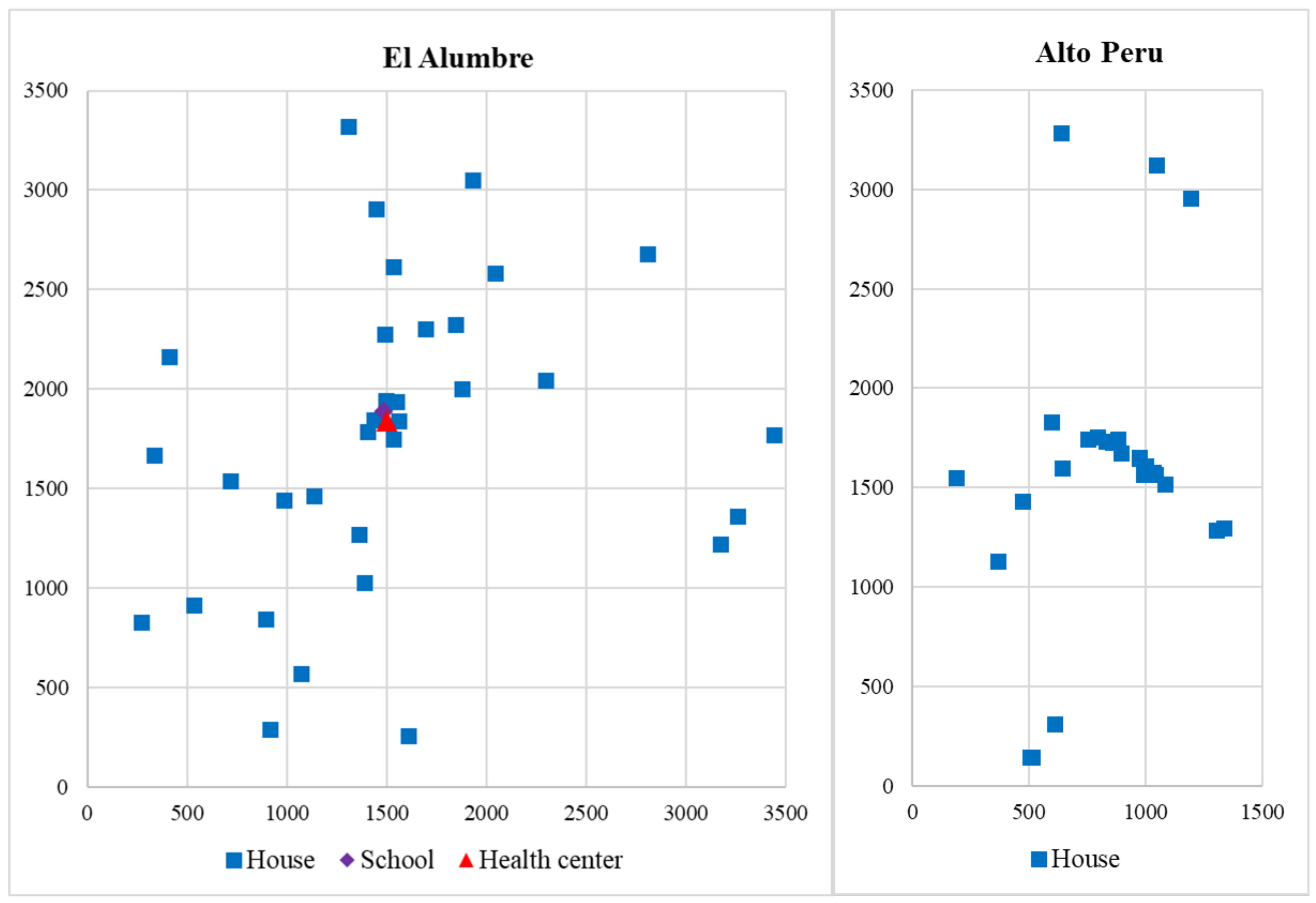
The two studied communities were El Alumbre (6°52′57″ S–78°26′23″ W) and Alto Peru (6°54′25″ S–78°37′24″ W) (Figure 4). The former had 33 houses, 1 school and 1 health center, widely dispersed. Alto Peru had 26 houses, 50% of them concentrated in 30% of the territory. The wind resource in both communities was variable; in some parts of the community, the wind resource was high, while other parts had low to moderate wind resource. The solar resource was highly significant, constant and the same for both communities.

Figure 4. Layout of the Peruvian communities.

4.4. Input Data

Table 1 summarizes the data used for evaluating the proposed solving procedure. The data are different for the three countries studied. Regarding the essential and improved demands, values were defined together with experts from each country, according to the specific needs of each region’s population. Based on these scenarios, the maximum (C^MAX) and minimum (C^MIN) costs for each community are calculated using the deterministic MILP model [36]. The other data were gathered from commercial catalogues, the literature review and consultations with project promoters. The models were solved with the ILOG CPLEX 12.6 on a 2.40 GHz, CPU Intel Core 15-1135G7 computer with 12 GB of RAM.

Table 1. Input data for each community and country.

Community		Ecuador		Mexico		Peru
		Suraka	Conambo	Tuzal	Villa del Rio	El Alumbre	Alto Peru
Demand Points	Demand points N	12	61	18	26	35	26
	Maximum distance LMAX (m)	500		500		500
Energy Demand	Essential EpMIN (Wh/day)	1000 (all)		100 (other) 750 (houses) 1500 (churches)		280 (houses) 975 (other)	280 (houses)
	Improved EpMAX (Wh/day)	1500 (all)		150 (other) 1125 (houses) 2250 (churches)		420 (houses) 1463 (other)	420 (houses)
Peak Power Demand	Essential PpMIN (W)	600 (all)		50 (other) 300 (houses) 750(churches)		200 (houses) 600 (school) 1000 (health c.)	200 (houses)
	Improved PpMAX (W)	900 (all)		75 (other) 450 (houses) 1125 (churches)		300 (houses) 900 (school) 1500 (health c.)	300 (houses)
Wind Turbines	Options A	n.a.		6		4
	Maximum number NA	n.a.		28		28
	Energy EApa (Wh/day)	n.a.		180 to 121,487		61 to 16,464
	Cost CAa (USD)	n.a.		1565 to 40,242		974 to 5132
PV Panels	Options S	1		5		4
	Maximum number NS	40		52		52
	Energy ESs (Wh/day)	1179		403 to 1048		217 to 652
	Nominal power PSs (W)	330		100 to 260		50 to 150
	Cost CSs (USD)	350		197 to 245		451 to 800
PV Controller	Options Z	2		4		4
	Peak power PZz (W)	480 to 2880		50 to 200		50 to 200
	Cost CZz (USD)	300 to 700		67 to 125		67 to 125
Batteries	Options B	2		4		4
	Capacity EBb (Wh)	1800 to 3600		24,422 to 63,360		1500 to 3000
	Cost CBb (USD)	300 to 850		132 to 387		225 to 325
	Discharge DB (u.f.)	0.60		0.60		0.60
	Self-sufficiency VB (days)	3		2		2
	Efficiency ηB (u.f.)	0.85		0.85		0.85
Inverters	Options I	2		5		4
	Peak power PIi (W)	600 to 3600		450 to 3000		300 to 3000
	Cost CIi (USD)	400 to 2000		60 to 582		377 to 2300
	Efficiency ηI	0.85		0.85		0.85
Meters	Cost CM (USD)	50		50		50
LV Lines	Options C	2		3		2
	Resistance RCc (Ω/m)	0.0016 to 0.0030		0.0017 to 0.0027		0.0017 to 0.0027
	Intensity ICc (A)	60 to 96		89 to 101		89 to 101
	Cost CCc (USD/m)	3.94 to 6.03		4.90 to 5.25		4.90 to 5.00
	Nominal voltage VN (V)	220		220		220
	Minimum voltage VMIN (V)	210		210		210
	Maximum voltage VMAX (V)	230		230		230
	Efficiency ηC (u.f.)	0.90		0.90		0.90

5. Results and Discussion

This section, first of all, discusses the results obtained for the six studied communities in regard to how balanced solutions were obtained with the proposed FMILP models (Section 5.1). Then, the two modeling assumptions (i.e., minimum satisfaction and average satisfaction) are compared to identify the most suitable one (Section 5.2).

5.1. Results for the Six Case Studies

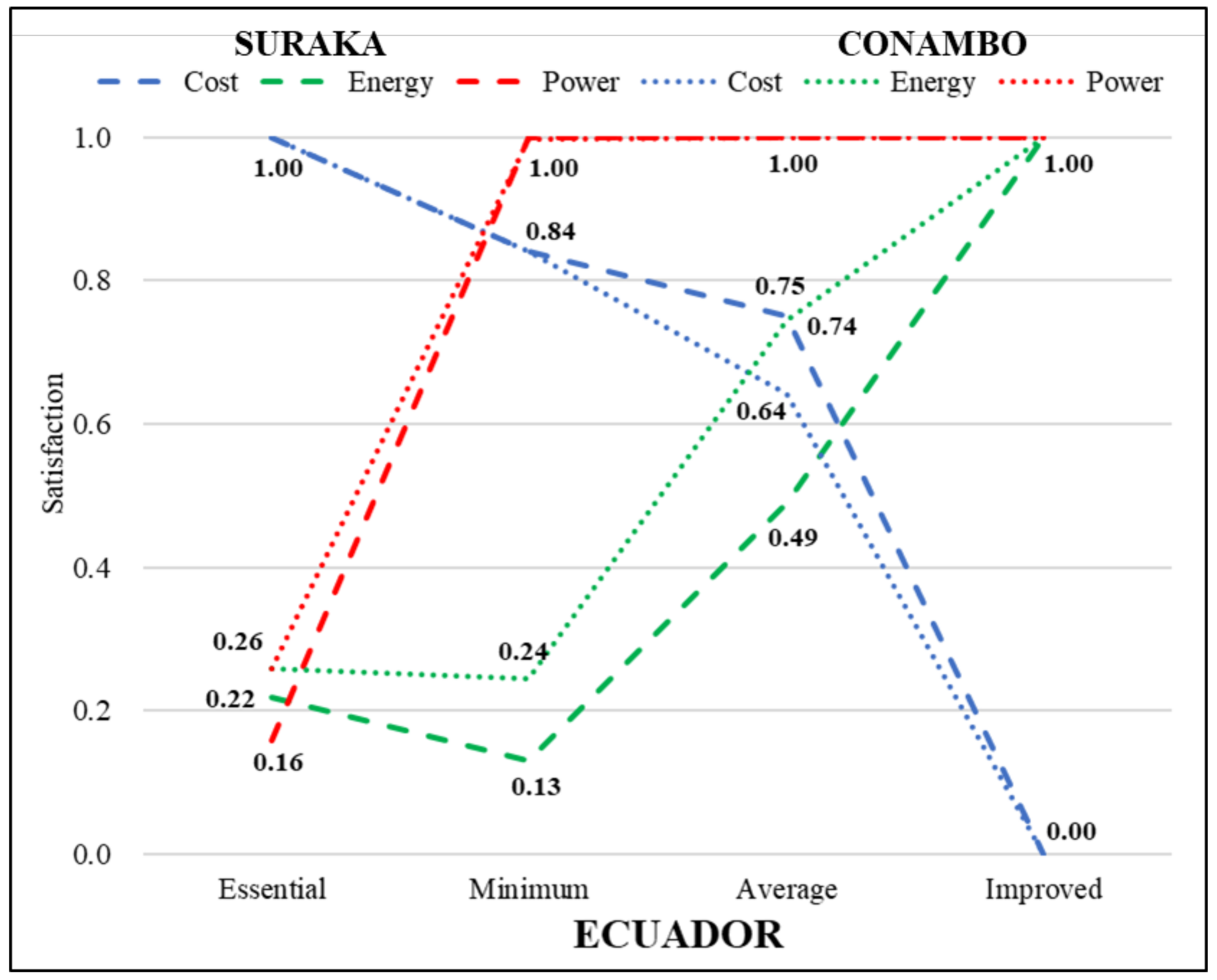
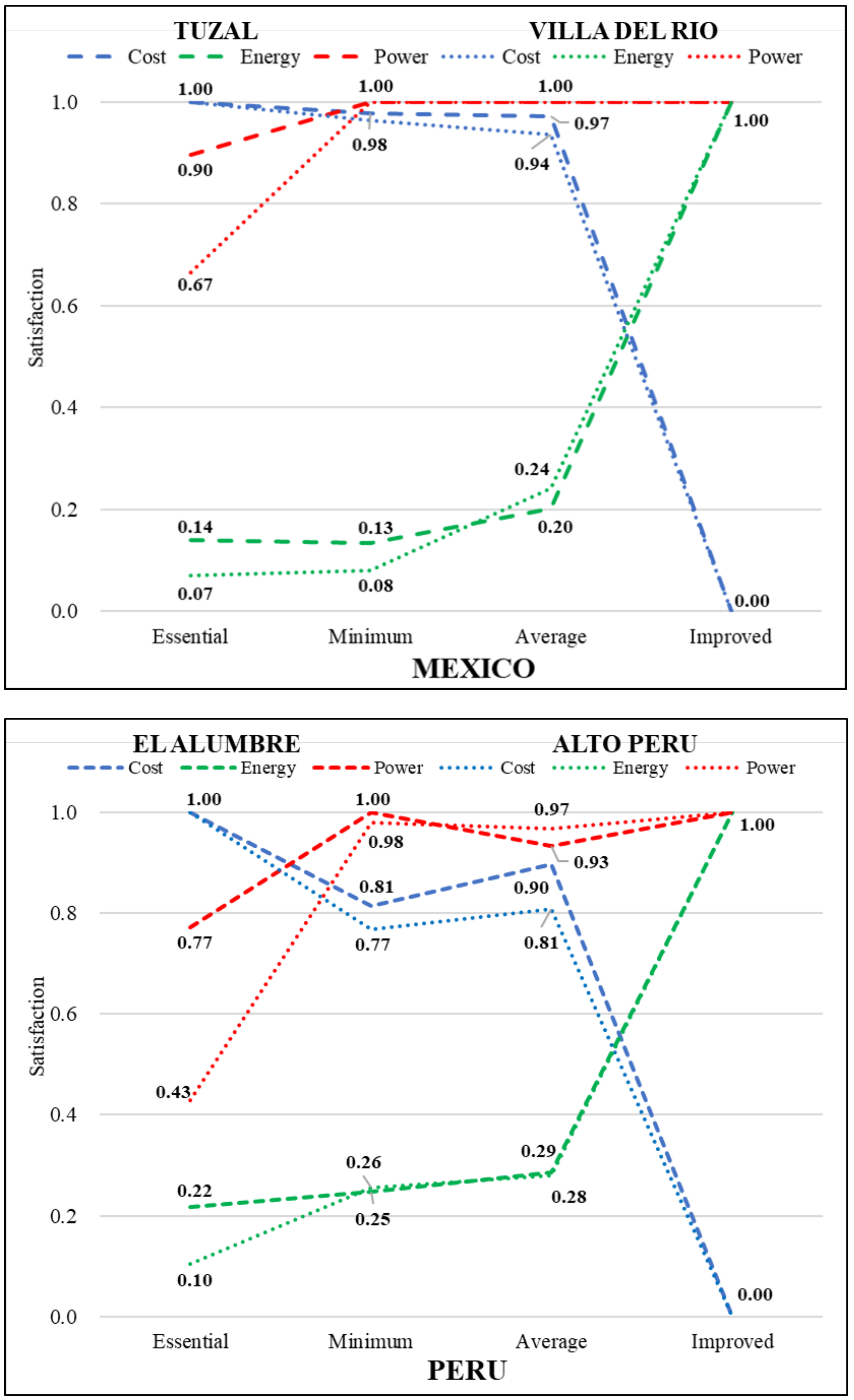
Figure 5 shows the results of satisfaction regarding the cost λ_C (blue), energy λ_E (green) and peak power λ_P (red) for the six studied communities. The results are organized in three images per country, using dashed (i.e., Suraka, Tuzal and El Alumbre) or dotted lines (i.e., Conambo, Villa del Rio and Alto Peru). The results are shown for the four solutions obtained in each community. The results of the deterministic MILP model are presented at the extremes of the figure: essential demand (top left) and improved demand (top right). The results of the FMILP models are presented in the middle: minimum satisfaction (mid-left) and average satisfaction (mid-right). Hence, for instance, in Suraka (Ecuador), Figure 5 shows the values of λ_C = 1.00, λ_E = 0.22 and λ_P = 0.16 obtained for the essential demand with the deterministic MILP model and λ_C = 0.84, λ_E = 0.13 and λ_P = 1.00 obtained with the minimum satisfaction FMILP model.

Figure 5. Results for the 6 case studies.

Regarding the MILP results, the essential demand solutions have full cost satisfaction and very low energy satisfaction with, occasionally, high power satisfaction. Indeed, the essential demand solutions were not limited to null energy and power satisfaction (equal to 0.0). The reason for this is the staggered nature of the equipment and economies of scale, which means that, in some cases, a higher energy and/or peak power demand than needed is supplied without increasing the cost. This varies depending on the community; for instance, in Tuzal the essential demand MILP model obtained an energy satisfaction of 0.14 and a power satisfaction of 0.90. In contrast, the energy satisfaction in Suraka was 0.22 and the peak power was 0.16. However, improved demand solutions always obtain full satisfaction for the energy and peak power and null satisfaction when it came to the cost.

Regarding the FMILP solutions, when compared to the essential demand solutions, they provided similar energy satisfaction (slightly lower or higher, depending on the community) but with significantly higher peak power satisfaction in exchange for slightly more expensive solutions. For instance, in Alto Peru energy satisfaction increased from 0.10 (essential) to 0.26 (minimum) or 0.28 (average) and the peak power from 0.43 (essential) to 0.98 (minimum) or 0.97 (average). These improvements were accomplished with a small reduction in the cost satisfaction from 1.00 (essential) to 0.77 (minimum) or 0.81 (average). When compared to the improved demand solutions, the FMILP solutions provided similar peak power satisfaction but less energy satisfaction to obtain a much higher cost satisfaction.

Thus, the results confirm that the solutions obtained with the FMILP were more balanced than those from the deterministic MILP. In general, the FMILP solutions compensate for a reduction in one of the satisfaction variables with an increase in one of the other two satisfaction indicators. Therefore, the use of the FMILP models reduces the negative effects of uncertainty and obtains robust and globally better solutions in terms of satisfaction.

It is also worth noting that, in all of the Ecuadorian and Mexican communities, the average satisfaction assumption showed results with an energy satisfaction and equal peak power satisfaction similar to the minimum satisfaction assumption, but the average assumption solutions had a higher cost. In contrast, the Peruvian communities showed the opposite situation. Therefore, the comparison between these two modeling assumptions is not straightforward and is further examined in Section 5.2.

5.2. Comparison of Assumptions

The above section showed the most balanced solutions obtained with the FMILP models rather than with the deterministic model. However, the discussion regarding the minimum satisfaction and the average satisfaction assumptions needs to be examined in more detail. In this regard, note that the objective functions of the FMILP models (see Equations (1) and (1’)) balance the cost satisfaction with the average of the energy and peak power satisfactions. Therefore, the comparison of assumptions in Figure 5 is not straightforward, since variations in cost satisfaction are not directly proportional to variations in energy or peak power satisfaction.

In order to deal with this, both assumptions were compared. Figure 6 shows the 12 solutions examined (i.e., six communities with two assumptions per community). For each solution, two values were calculated: the minimum satisfaction objective function (1), top image; the average satisfaction objective function (1’), bottom image. For instance, in Suraka, the minimum satisfaction FMILP was solved, and the obtained value of the objective function (1) was 1.40 (top). For this solution, the value of the other objective function (1’) was calculated manually, obtaining 1.41 (bottom). Additionally, also for Suraka, the average satisfaction FMILP was solved, and the obtained value of the objective function (1’) was 1.49 (bottom). For this solution, the value of the other objective function (1) was calculated manually, obtaining 1.25 (top).

Figure 6. Comparison of the objective function values between assumptions.

As shown in Figure 6, logically, the minimum satisfaction solutions (red bars) in the top image are higher than the average satisfaction solutions (green bars) for all of the communities; the opposite occurs in the bottom image. However, the differences between bar sizes were significantly higher for the minimum satisfaction objective function (top) than for the average satisfaction objective function (bottom). For instance, in Conambo the difference was 0.19 for the minimum satisfaction objective function (1.33 vs. 1.14), while it was only 0.05 for the average satisfaction objective function (1.46 vs. 1.51). In El Alumbre, the differences were even higher: 0.54 (1.44 vs. 0.90) and 0.07 (1.44 vs. 1.51), respectively. Consequently, the average satisfaction solutions logically obtained top values for their objective function (1’), but their performance on the minimum satisfaction objective function (1) was limited. In contrast, the minimum satisfaction solutions are more recommendable, since they logically obtained the top values in their objective function (1) and, in addition, they achieved close-to-top values in terms of the average satisfaction objective function (1’).

In short, as a recommendation for project promoters willing to design an electrification project for a community without electricity, where demand is difficult to estimate, the authors suggest solving the two proposed FMILP models; the obtained solutions would balance, in a different way, the satisfaction regarding the cost, energy and peak power. Then, a choice can be made between these two solutions based on the very specific details of each one, taking into account the opinion of experts and the community. However, the general recommendation is that the minimum satisfaction FMILP model obtains globally better solutions.

6. Conclusions

Estimating demand in settlements accessing electricity for the first time is complex and subject to uncertainty. With the current tools, project developers must obtain a unique electrification solution (the quality of which logically depends on the estimated demand) or examine different demand values (each one leading to a different solution with a different cost) and then manually analyze the best one. In both cases, the decision-making process has limitations that might impact on the performance of the finally implemented solution. To overcome this situation, this work developed a tool that enables satisfaction with regard to the project cost and the energy and peak power supplied to end users to be balanced.

In order to do so, a novel FMILP model was proposed, based on a modeling approach tested in the literature as efficient, to balance the cost satisfaction and the energy and peak power satisfaction. Hence, project promoters have a powerful tool for designing rural electrification projects in developing countries, combining wind and PV technologies as well as microgrids and individual systems, while taking into account the uncertainty in demand estimation. Rather than being subject to a specific demand value, the novel FMILP model enables a range of values to be specified and the most balanced solution is returned. In addition, two assumptions were modeled: maximizing the minimum satisfaction (focus on the least satisfied demand point) and maximizing the average satisfaction (global satisfaction of all points).

The validation of the proposed solving procedure was performed using six case studies from three Latin American countries (i.e., Ecuador, Mexico and Peru). In particular, two demand scenarios were defined: an essential demand, to cover basic end-user needs, and an improved demand, above which solutions would be considered too expensive. The FMILP solutions (one for each assumption) were compared with those obtained with a deterministic MILP model. The results show that the MILP models led to low-supply or expensive solutions, while the FMILP models allowed for a balance between the cost, energy and peak power to be achieved. Finally, the results for the FMILP models under the two assumptions were compared. Although the two models can be easily solved and the best option can then be selected based on specific details, the minimum satisfaction FMILP model is recommended in the case of promoters wanting a unique solution, since it obtains the top values for minimum satisfaction as well as close-to-top values for average satisfaction.

Prior to this work, project promoters could obtain a unique electrification solution, subject to the quality of the estimation of end-users’ demand. In the case of wanting to test different demand scenarios, they had to solve each one manually through the deterministic MILP model and then select the best one after a discussion that might not be straightforward. In contrast, with the proposed FMILP models, this process is simplified. Now, project promoters only have to delimit the range of demand values, and the most balanced solution is directly obtained with each of the two FMILP models developed.

References

- United Nations (UN). 2030 Agenda for Sustainable Development; United Nations: New York, NY, USA, 2015. [Google Scholar]
- Eras-Almeida, A.A.; Egido-Aguilera, M.A. What is still necessary for supporting the SDG7 in the most vulnerable contexts? Sustainability 2020, 12, 7184. [Google Scholar] [CrossRef]
- International Energy Agency (IEA). Global Status Report. Towards a Zero-Emission, Efficient and Resilient Buildings and Construction Sector; International Energy Agency: Paris, France, 2018; ISBN 978-92-807-3729-5. [Google Scholar]
- Madriz-Vargas, R.; Bruce, A.; Watt, M. The future of community renewable energy for electricity access in rural Central America. Energy Res. Soc. Sci. 2018, 35, 118–131. [Google Scholar] [CrossRef]
- Mehrjerdi, H. Modeling, integration, and optimal selection of the turbine technology in the hybrid wind-photovoltaic renewable energy system design. Energy Convers. Manag. 2020, 205, 112350. [Google Scholar] [CrossRef]
- Sima, C.A.; Lazaroiu, G.C.; Dumbrava, V.; Tirsu, M. A hybrid system implementation for residential cluster. In Proceedings of the 2017 International Conference on Electromechanical and Power Systems, Iasi, Romania, 11–13 October 2017; pp. 275–280. [Google Scholar] [CrossRef]
- Hirsch, A.; Parag, Y.; Guerrero, J. Microgrids: A review of technologies, key drivers, and outstanding issues. Renew. Sustain. Energy Rev. 2018, 90, 402–411. [Google Scholar] [CrossRef]
- Domenech, B.; Ferrer-Martí, L.; Pastor, R. Comparison of various approaches to design wind-PV rural electrification projects in remote areas of developing countries. WIREs Energy Environ. 2019, 8, e332. [Google Scholar] [CrossRef]
- Mavromatidis, G.; Orehounig, K.; Carmeliet, J. A review of uncertainty characterization approaches for the optimal design of distributed energy systems. Renew. Sustain. Energy Rev. 2018, 88, 258–277. [Google Scholar] [CrossRef]
- Anoune, K.; Bouya, M.; Astito, A.; Abdellah, A.B. Sizing methods and optimization techniques for PV-wind based hybrid renewable energy system: A review. Renew. Sustain. Energy Rev. 2018, 93, 652–673. [Google Scholar] [CrossRef]
- Liu, Y.; Yu, S.; Zhu, Y.; Wang, D.; Liu, J. Modeling, planning, application and management of energy systems for isolated areas: A review. Renew. Sustain. Energy Rev. 2018, 82, 460–470. [Google Scholar] [CrossRef]
- Lyden, A.; Pepper, R.; Tuohy, P.G. A modelling tool selection process for planning of community scale energy systems including storage and demand side management. Sustain. Cities Soc. 2018, 39, 674–688. [Google Scholar] [CrossRef]
- Soukeyna, M.; Ramdhane, I.B.; Ndiaye, D.; Elmamy, M.; Menou, M.; Yahya, A.M.; Mahmoud, A.K.; Youm, I. Feasibility analysis of hybrid electricity generation system by HOMER for Mauritanian northern coast. Int. J. Phys. Sci. 2018, 13, 120–131. [Google Scholar] [CrossRef]
- Raji, A.K.; Luta, D.N. Modeling and optimization of a community microgrid components. Energy Procedia 2019, 156, 406–411. [Google Scholar] [CrossRef]
- Sima, C.A.; Popescu, M.O.; Popescu, C.L.; Alexandru, M.; Popa, L.B.; Dumbrava, V.; Panait, C. Energy management of a cluster of buildings in a university campus. In Proceedings of the 2021 12th International Symposium on Advanced Topics in Electrical Engineering, Bucharest, Romania, 25–27 March 2021. [Google Scholar] [CrossRef]
- Rojas-Zerpa, J.C.; Yusta, J.M. Application of multicriteria decision methods for electric supply planning in rural and remote areas. Renew. Sustain. Energy Rev. 2015, 52, 557–571. [Google Scholar] [CrossRef]
- Bhagavathy, S.M.; Pillai, G. PV microgrid design for rural electrification. Designs 2018, 2, 33. [Google Scholar] [CrossRef]
- García-Villoria, A.; Domenech, B.; Ferrer-Martí, L.; Juanpera, M.; Pastor, R. Ad-hoc heuristic for design of wind-photovoltaic electrification systems, including management constraints. Energy 2021, 212, 118755. [Google Scholar] [CrossRef]
- Ciupageanu, D.A.; Barelli, L.; Lazaroiu, G. Real-time stochastic power management strategies in hybrid renewable energy systems: A review of key applications and perspectives. Electr. Power Syst. Res. 2020, 187, 106497. [Google Scholar] [CrossRef]
- Riva, F.; Ahlborg, H.; Hartvigsson, E.; Pachauri, S.; Colombo, E. Electricity access and rural development: Review of complex socio-economic dynamics and causal diagrams for more appropriate energy modelling. Energy Sustain. Dev. 2019, 43, 203–223. [Google Scholar] [CrossRef]
- Peters, J.; Sievert, M.; Toman, M.A. Rural electrification through mini-grids: Challenges ahead. Energy Policy 2019, 132, 27–31. [Google Scholar] [CrossRef]
- Good, N.; Ellis, K.A.; Mancarella, P. Review and classification of barriers and enablers of demand response in the smart grid. Renew. Sustain. Energy Rev. 2017, 72, 57–72. [Google Scholar] [CrossRef]
- Ozturk, H.K.; Canyurt, O.E.; Hepbasli, A.; Utlu, Z. An application of genetic algorithm search techniques to the future total exergy input/output estimation. Energy Sources Part A 2006, 28, 715–725. [Google Scholar] [CrossRef]
- Azadeh, A.; Ghaderi, S.F.; Tarverdian, S.; Saberi, M. Integration of artificial neural networks and genetic algorithm to predict electrical energy consumption. Appl. Math. Comput. 2007, 186, 1731–1741. [Google Scholar] [CrossRef]
- Badurally Adam, N.R.; Dauhoo, M.Z.; Elahee, M.K. A simulated-based genetic algorithm for the forecasting of monthly peak electricity demand. Int. J. Oper. Res. 2017, 28, 164–182. [Google Scholar] [CrossRef]
- Badurally Adam, N.R.; Elahee, M.K.; Dauhoo, M.Z. Forecasting of peak electricity demand in Mauritius using the non-homogeneous Gompertz diffusion process. Energy 2011, 36, 6763–6769. [Google Scholar] [CrossRef]
- Domenech, B.; Ferrer-Martí, L.; Pastor, R. Hierarchical methodology to optimize the design of stand-alone electrification systems for rural communities considering technical and social criteria. Renew. Sustain. Energy Rev. 2015, 51, 182–196. [Google Scholar] [CrossRef][Green Version]
- Suganthi, L.; Iniyan, S.; Samuel, A. Applications of fuzzy logic in renewable energy systems—A review. Renew. Sustain. Energy Rev. 2015, 48, 585–607. [Google Scholar] [CrossRef]
- Onar, S.C.; Oztaysi, B.; Otay, İ.; Kahraman, C. Multi-expert wind energy technology selection using interval-valued intuitionistic fuzzy sets. Energy 2015, 90, 274–285. [Google Scholar] [CrossRef]
- Li, G.; Sun, W.; Huang, G.H.; Lv, Y.; Liu, Z.; An, C. Planning of integrated energy-environment systems under dual interval uncertainties. Int. J. Electr. Power 2018, 100, 287–298. [Google Scholar] [CrossRef]
- Mohammadi, M.; Noorollahi, Y.; Mohammadi-ivatloo, B. Fuzzy-based scheduling of wind integrated multi-energy systems under multiple uncertainties. Sustain. Energy Technol. Assess. 2020, 37, 100602. [Google Scholar] [CrossRef]
- Vahedipour-Dahraie, M.; Rashidizadeh-Kermani, H.; Anvari-Moghaddam, A.; Siano, P. Risk-averse probabilistic framework for scheduling of virtual power plants considering demand response and uncertainties. Int. J. Electr. Power 2020, 121, 106126. [Google Scholar] [CrossRef]
- Wang, J.; Qi, X.; Ren, F.; Zhang, G.; Wang, J. Optimal design of hybrid combined cooling, heating and power systems considering the uncertainties of load demands and renewable energy sources. J. Clean. Prod. 2021, 281, 125357. [Google Scholar] [CrossRef]
- Hossain, M.A.; Chakrabortty, R.K.; Ryan, M.J.; Pota, H.R. Energy management of community energy storage in grid-connected microgrid under uncertain real-time prices. Sustain. Cities Soc. 2021, 66, 102658. [Google Scholar] [CrossRef]
- Galleguillos-Pozo, R.; Domenech, B.; Ferrer-Martí, L.; Pastor, R. Design of stand-alone electrification systems using fuzzy mathematical programming approaches. Energy 2021, 228, 120639. [Google Scholar] [CrossRef]
- Ferrer-Martí, L.; Domenech, B.; García-Villoria, A.; Pastor, R. A MILP model to design hybrid wind-photovoltaic isolated rural electrification projects in developing countries. Eur. J. Oper. Res. 2013, 226, 293–300. [Google Scholar] [CrossRef]
- Pillot, B.; Muselli, M.; Poggi, P.; Dias, J.B. Historical trends in global energy policy and renewable power system issues in Sub-Saharan Africa: The case of solar PV. Energy Policy 2019, 127, 113–124. [Google Scholar] [CrossRef]
- López-González, A.; Domenech, B.; Gómez-Hernández, D.; Ferrer-Martí, L. Renewable microgrid projects for autonomous small-scale electrification in Andean countries. Renew. Sustain. Energy Rev. 2017, 79, 1255–1265. [Google Scholar] [CrossRef]
- Bilgen, B. Application of fuzzy mathematical programming approach to the production allocation and distribution supply chain network problem. Expert Syst. Appl. 2010, 37, 4488–4495. [Google Scholar] [CrossRef]
- Mendel, J.M.; Korjani, M.M. A new method for calibrating the fuzzy sets used in fsQCA. Inf. Sci. 2018, 468, 155–171. [Google Scholar] [CrossRef]
- Gómez-Hernández, D.F.; Domenech, B.; Moreira, J.; Farrera, N.; López-González, A.; Ferrer-Martí, L. Comparative evaluation of rural electrification project plans: A case study in Mexico. Energy Policy 2019, 129, 23–33. [Google Scholar] [CrossRef]
Publisher’s Note: MDPI stays neutral with regard to jurisdictional claims in published maps and institutional affiliations. |
© 2022 by the authors. Licensee MDPI, Basel, Switzerland. This article is an open access article distributed under the terms and conditions of the Creative Commons Attribution (CC BY) license (https://creativecommons.org/licenses/by/4.0/).