1. Introduction
Experimental designs were introduced firstly in agricultural projects. Industrial and laboratory researchers were inspired to adopt them into clinical trials of pharmaceuticals in humans because of their distinction in monitoring the experimental process to minimize errors. A clinical trial’s primary purpose is to find the optimum medical treatment by comparing the benefits of competing therapies at minimal costs and within a short period. Doing so with the least possible errors is highly critical [
1].
The first clinical trial designs utilized classical experimental designs. According to medical and physiological science progress, there was a need to change some elements during the trial process. The sample size could be modified, some trials could be terminated early, or the trial stages adjusted; the classical analysis cannot accommodate these modifications. Therefore, adaptive designs have been developed. An adaptive design is a method that involves modification of a current trial’s design or statistical procedure in response to the data generated from the trials. In addition, they allow investigators to identify the best treatment under study without compromising its validity and integrity [
2]. The types of adaptive design methods generally considered in clinical trials include an adaptive treatment switching design, a group sequential design, a biomarker-adaptive design, an adaptive randomization design, a drop-the-losers design, a sample size re-estimation design, and a hypothesis-adaptive design [
2].
An interim analysis (a group sequential design) is one of the most popular options. Using interim analysis has several benefits that can be loosely categorized into ethical, administrative, and economic categories. On the other hand, a group sequential design is morally imperative to control the results of clinical trials, including those involving human subjects, to minimize individual risks [
3].
Since group sequential testing procedures became widely used in medical experiments. The procedures were crucial to be developed by researchers to generalize and modify procedures for varying circumstances. By way of example, Maurer and Bretz developed a class of group-sequential-weighted Bonferroni procedures with multiple endpoints, for which the correlations of sequential statistics are used. Consequently, the power was increased, while the family-wise error rate was effectively controlled [
4]. On the other hand, Yiyong Fu presented follow-up work to Maurer and Bretz, proposing a Holm-type step-down exact parametric procedure for situations in which correlations are unknown. Further, he briefly outlined an extension of the partially parametric Seneta–Chen method that is naturally a group sequential design [
5]. Zhenming Shun examined an approach that combined sample size re-estimation, a negative stop (stochastic curtailment), and group sequential analysis in a single interim analysis conducted with normal data [
6].
Urach and Posch also considered an approach to improve critical boundaries for multi-arm experiments by using multi-arm group sequential designs with a simultaneous stopping rule. The resulting designs are also intended to optimize their boundaries’ shape and determine their operating characteristics [
7].
Most researchers recently adopted well-known procedures, such as the O’Brien and Fleming, Pocock, and Haybittle–Peto procedures [
8].
For the development of group sequential testing procedures, O’Brien and Fleming (1979) provided a primary inspiration in this field [
9], since they presented a direct and valuable group sequential testing procedure to compare two treatments in clinical trials. When one treatment performs better than the other, the trial is terminated using a smaller sample, where the procedure offers the same Type I error and power rates as a fixed one-stage chi-square test for categorical data.
The usage of this procedure can be seen in several medical studies. For example, Motzer used the O’Brien and Fleming stopping boundaries to end his experiment, entitled “efficacy of everolimus in advanced renal cell carcinoma”, early [
10]. In addition, Goldberg’s study was stopped after 50% of patients responded to his study, entitled “randomized controlled trial of fluorouracil plus leucovorin, irinotecan, and oxaliplatin combinations in patients with previously untreated metastatic colorectal cancer.” [
11]. Furthermore, Baily used it in their designed trial to examine whether male circumcision was protective against HIV infection [
12]. In addition to this, Marcus terminated the Gallium trials earlier by using the O’Brien and Fleming interim analysis. These trials involved follicular lymphoma patients [
13].
The O’Brien and Fleming multiple testing procedure has been modified several times by researchers, such as Kung-Jong Lui, who examined the performance of the O’Brien–Fleming multiple testing procedure when intraclass correlations were presented [
14]. Along with this, he enhanced the original procedure by increasing the number of stages and the number of treatments. Moreover, in Hammouri’s study (2013), the stopping bounds of the O’Brien–Fleming procedure were corrected, and the validation was verified after the correction was applied. When she reviewed the multiple testing methods’ stopping bounds, a non-monotonicity problem in the critical values was noticed. The solution was that the number of simulations producing critical values was increased compared to the number of simulations in the initial process. That facilitated the procedure with monotonic critical values. Indeed, when more iterations were added to the simulation, the critical values got larger and made the rejection of the null hypotheses harder, leading to control of the Type I error. Furthermore, the O’Brien–Fleming procedure was updated in Hammouri’s work to make it more flexible via three implementations. Each implementation was executed separately. Two of these three implementations are the optimal allocation, where the idea is to allocate more patients to the better treatment after each interim analysis. The other implementation allows for different sample weights for different stages instead of an equal sample size within the various stages [
15].
O’Brien and Fleming (1979) procedure was built using balanced randomization. In this paper, the randomization will be changed to an unbalanced one. Randomization is known to eliminate potential bias and confounders from clinical trials. It is the standard gold method for statistical power. One asset that can be used with multiple-testing methods is unbalanced randomization, which seems favorable due to several constraints. Scientists preferred to use optimal proportions to solve two problems: minimize the number of failures with the power, which is fixed, and maximize the homogeneity test’s power with a fixed sample size [
16].
Optimal experimental design can be obtained by carefully allocating treatment to study subjects; subjects are randomized to less toxic or more effective treatment regimens. There are many different optimal allocation designs for clinical trials available in the literature. For example, response-adaptive randomization (RAR) design is used to find the optimal allocations for clinical trials with multiple endpoints. RAR designs can be traced to Thompson (1933), Robbins (1952), and Zelen (1969) [
17,
18,
19]. An example of optimal allocation of patients with RAR designs is the randomized play-the-winner rule. Hu and Rosenberger’s (2003) method for optimal RAR procedures involved formalizing the objectives and deriving the optimal allocation proportion for binary responses [
20]. Thus, the OWMP will use optimal allocation instead of equal allocation.
One more change will be including the unequal weights in the subsamples. In the literature, Lehmacher and Wassmer (1999) proposed a method that uses adaptive sample size calculations in group sequential trials; the method is for the adaptive planning of sample sizes for group sequential clinical trials [
21]. The method was for group sequential trials that combined the results from separate stages using the normal inverse method. The method allows for data-driven reassessments of the sample size without exaggerating the Type I error rate. Next, Proschan and Chi suggested two different two-stage adaptive designs that keep the Type I error rate steady. Proschan’s adaptive design is essential to accomplish an anticipated statistical power while restraining the maximum sample size. Furthermore, Chi’s adaptive design consists of the main stage with adequate power to reject the null hypothesis and an implementation stage that permits increasing the sample size if the actual effect size is smaller than anticipated [
22].
Usually, when a new method is developed from previous methods, a Monte Carlo simulation is used to validate the new one. A Monte Carlo simulation is a system for doing what-if analysis that allows users to measure the reliability of different analyses’ results and inferences. In the 1940s, Jon von Neumann and Ulam developed the Monte Carlo simulation, a handy statistical tool for evaluating multiple scenarios in-depth to study uncertain situations. Additionally, simulation studies are associated with pseudo-random sampling, which creates data from computer experiments. Since data generation processes are known in advance, simulation studies have the advantage of understanding and studying the performance of statistical methods [
23,
24,
25].
In this current study, a new method has been developed that incorporates optimal allocation and varying sample weights at different stages, together with the O’Brien and Fleming multiple testing procedure named the optimal weighted multiple-testing procedure. Furthermore, Type I error and power have been studied to determine if the new method is effective using Monte Carlo simulations.
3. The Proposed Procedure OWMP
3.1. The New Methodology
Using the corrected critical values and then combining the procedure with the optimal allocation together with different sample weights, the procedure was enhanced for efficiency.
The method is suggested as follows:
There is a total sample size , and a number of stages , as well as the sample weights {, …, } and α, which are all chosen in advance. where sample weights {, …, } are used to get each stage sample size , where 0 and ∑= 1. For each , the sample size for each stage is calculated as follows:
For , is calculated as = round (× N), if is even. Otherwise = round ( N) + 1; because equal allocation is used in the first stage. Furthermore, equal allocation is used in other stages when the optimal ratio equals zero or one.
For the last stage , to cover the rounding that is used in the previous stages.
Now, for , treatments A and B are assigned to and subjects, respectively. Where and must be equal and ( = + ). For , A stage with subjects are divided to and subjects assigned to treatment A and B, respectively.
Where
with
=
, and
and
are success rates from the previous stage for treatment A, and treatment B, respectively [
26]. Therefore,
=
−
for all
. Then for each stage
subjects are randomized, and their measurements are observed. Each subsample will be added to the previous subsamples for the same treatment. At that time
is calculated. Where
is the usual Pearson chi-square statistic.
is compared to
where α is the size of the test, and
is a critical value from
Table 2. If
, then the study is terminated, and the null hypothesis is rejected. Otherwise
and
, the study is terminated, and the null hypothesis fails to be rejected. However, if
, and
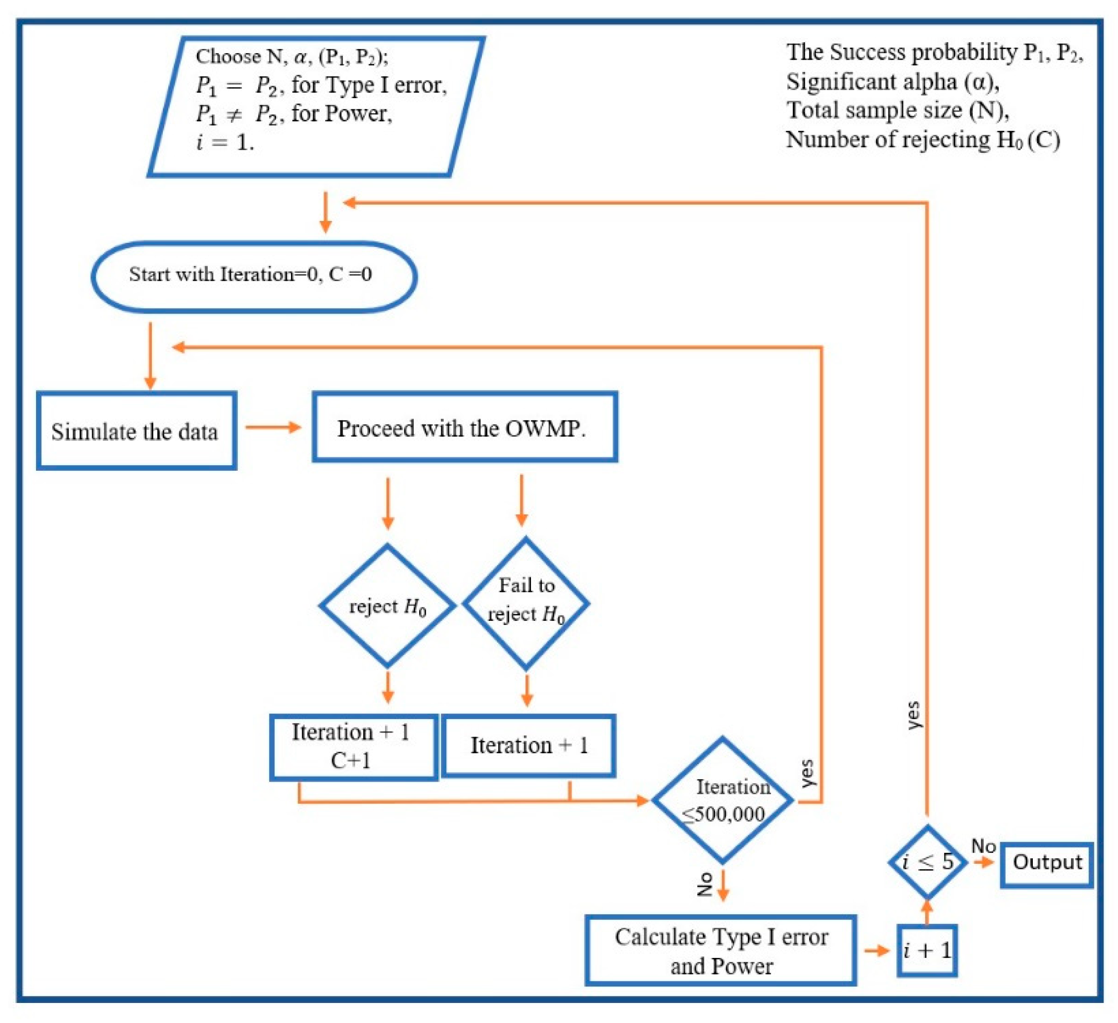
, the procedure proceeds to the next stage. The method is illustrated in
Figure 2.
3.2. Type I Error and Power to Validate the OWMP
This section utilizes Monte Carlo simulations to investigate the Type I error and the power of the OWMP. A theoretical approach can, in many situations, be challenging to implement, much less to find a precise answer. Using Monte Carlo simulations can provide an alternative to theoretical analysis. In the case of O’Brien and Fleming, they used an approximation distribution, so they used simulation to show that a fixed one-stage chi-square test has the same Type I error rate and power as theirs. So, the same approach was used in the current work, and all simulations were run using SAS software.
3.2.1. Testing Type I Error Algorithm
In order to calculate the Type I error, success probabilities
,
and critical value
were chosen with different sample sizes for all values of
. In each case of
, both subsamples are generated from the same binomial distribution with the same success rate. Assess if the OWMP fails to reject the null hypothesis of no significant difference between groups or accepts that there is a significant difference between groups. The latter result is causing a Type I error. After repeating this 500,000 times, the proportion of rejecting
is calculated and this represents the Type I error (
Figure 3).
3.2.2. Result of Testing Type I Error
Simulations were run to calculate the Type I error for the multiple-testing procedure using SAS code. Sample sizes of various scenarios were considered. Almost identical results were obtained for all sample sizes that were used. Compared to the usual chi-square, the OWMP maintained, if not decreased, the Type I error. With higher
, it was observed that the decreasing trend intensified. The reason is that, with a larger
, the usual chi-square statistic is multiplied by a factor less than one and it is compared with a larger critical value. So, rejecting
becomes harder. For illustration, results for sample size 250 with
and sample size of 300 with
were reported in
Table 3 and
Table 4, respectively.
In the first case, with and a sample size of 250, when , the values for the Type I error ranged between 0.0499 and 0.0503. While the number of increased, the values of the Type I error monotonically decreased, where the values are between 0.0415 and 0.0438 at , which is less than 0.05, which is an even more acceptable error than the usual chi-square procedure.
Likewise, various sample sizes were used to compute the Type I error values resulting in the same conclusion. For example, the Type I error values with a sample size of 80 and 580 were calculated. The values ranged between 0.0418 and 0.0506, 0.0438 and 0.0507, respectively, for , and all values of .
Similarly, Type I error values displayed a monotonic behavior with , since the values ranged between 0.0093 and 0.0104, in the first case, with . A decrease in Type I errors has also been noted, while a rise in values has been applied, which is satisfactory since the errors do not exceed 0.0104.
Furthermore, other samples were calculated in order to determine the Type I error values. For example, values for and sample sizes of 80 and 630 were calculated. It has been observed that the error values ranged from 0.0090 to 0.0101 and from 0.0084 to 0.0101, respectively, indicating that the OWMP is working effectively regarding Type I errors.
3.2.3. Testing Power Algorithm
To evaluate the power values, a probability value was chosen for all cases and a different success probability was chosen from the set {0.15, 0.2, 0.25, 0.3} with and the number of interim analyses being 500,000, and the corrected O’Brien and Fleming critical values Sample sizes were chosen such that the sample guaranteed the power values to be equal to 0.8 using the usual chi-square test power calculation.
In each case of
, the subsamples are generated from two different binomial distributions with different
to make sure that the alternative hypothesis is true. Then, the OWMP was used to examine if
(that there is a difference between the two groups) is rejected, or a significant difference is found and
is accepted. After repeating this 500,000 times, the proportion of accepting
is computed, and this is the power rate (because
was assured to be true). The process of computing the power is illustrated in
Figure 3.
3.2.4. Result of Testing Power
The OWMP was able to preserve acceptable power values with the new implementation. The OWMP was studied for α = 0.05 and 0.01, and several values of
that guaranteed a power of 0.8, and SAS code was used to calculate the power for each case with a variety of
values.
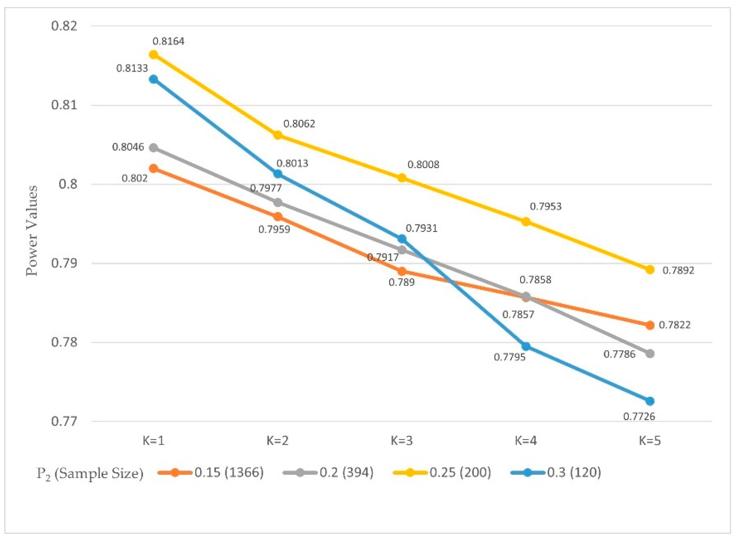
Table 5 and
Table 6,
Figure 4 and
Figure 5 show the power values from the 500,000 simulations.
The probability value was fixed, and the power rates with various values for , and , were studied.
The sample sizes 1366, 396, 200, and 120 for , and 2032, 588, 292, and 182 for were used to ensure that the power values were 0.8.
It was noticed that with the results for the power values with were between 0.8046 and 0.8164. Then, the values showed a decreased behavior when the values of were increased because the power values, when were between 0.7726 and 0.7892, with marginal errors not more than 0.0274 between the power values and the 0.8.
The power values with and were between 0.8010 and 0.8113. It was further found that by comparing the power results with the values of the power values monotonically decreased as values increased. However, the power values when were between 0.7840 and 0.7888 with marginal errors not more than 0.0160.
In both values, the marginal errors are negligible to be considered.
3.3. Calculating Rejection Rates for Each Stage
In this section, for each stage, the null hypothesis rejection rates, along with the sample sizes required to reject it were calculated.
3.3.1. Calculating Rejection Rates for Each Stage When Is True, and the Difference Is Presented
The rejections were calculated with a standard power value of 0.8, with the probabilities of success of
and
with
and the sample size was
.
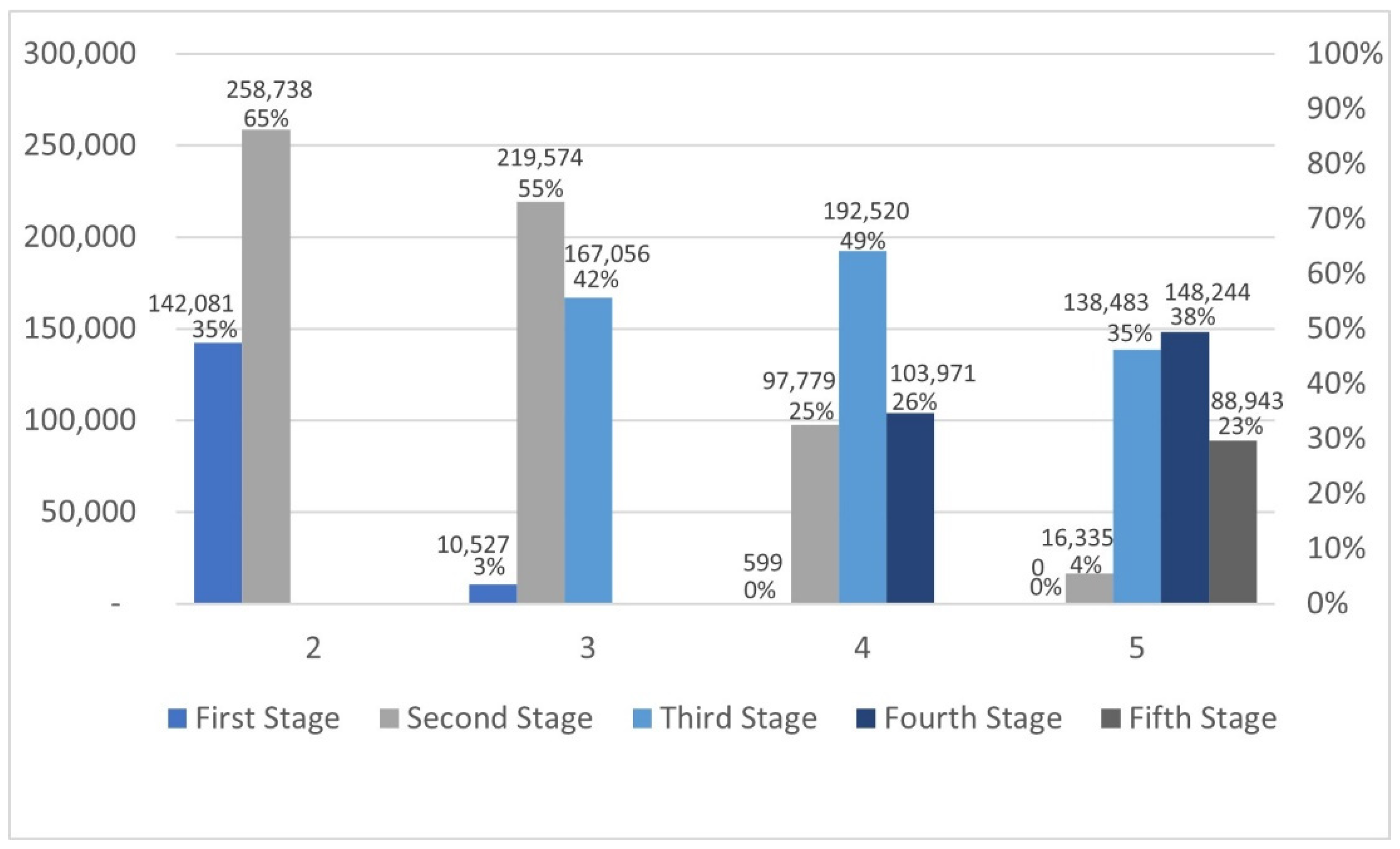
Table 7 and
Figure 6 demonstrate the needed sample size and the number of rejections of
occurring at stage
with 500,000 iterations.
With of rejections occurred in the first stage, and 65% occurred in the second stage, so the whole sample size was not needed to reject the hypothesis in more than a third of the cases. Based on , the sample size needed to reject the hypothesis in the second stage was 488, which resulted in a 55% rejection rate. The highest rejection rate with was in the third stage with 49%, and the needed sample size was 530 to reject .
In addition, in 74% of the cases, the whole sample was not needed. At , the highest rejection percentage was 38%, with a 530 sample size, and the highest percentage was at the fourth stage. Rejection occurred in 77% of cases earlier in the process.
3.3.2. Calculating Rejection Rates for Each Stage When Is True, and the Difference Is Not Presented
The rejections were calculated with
and the sample size was
. Based on 500,000 iterations,
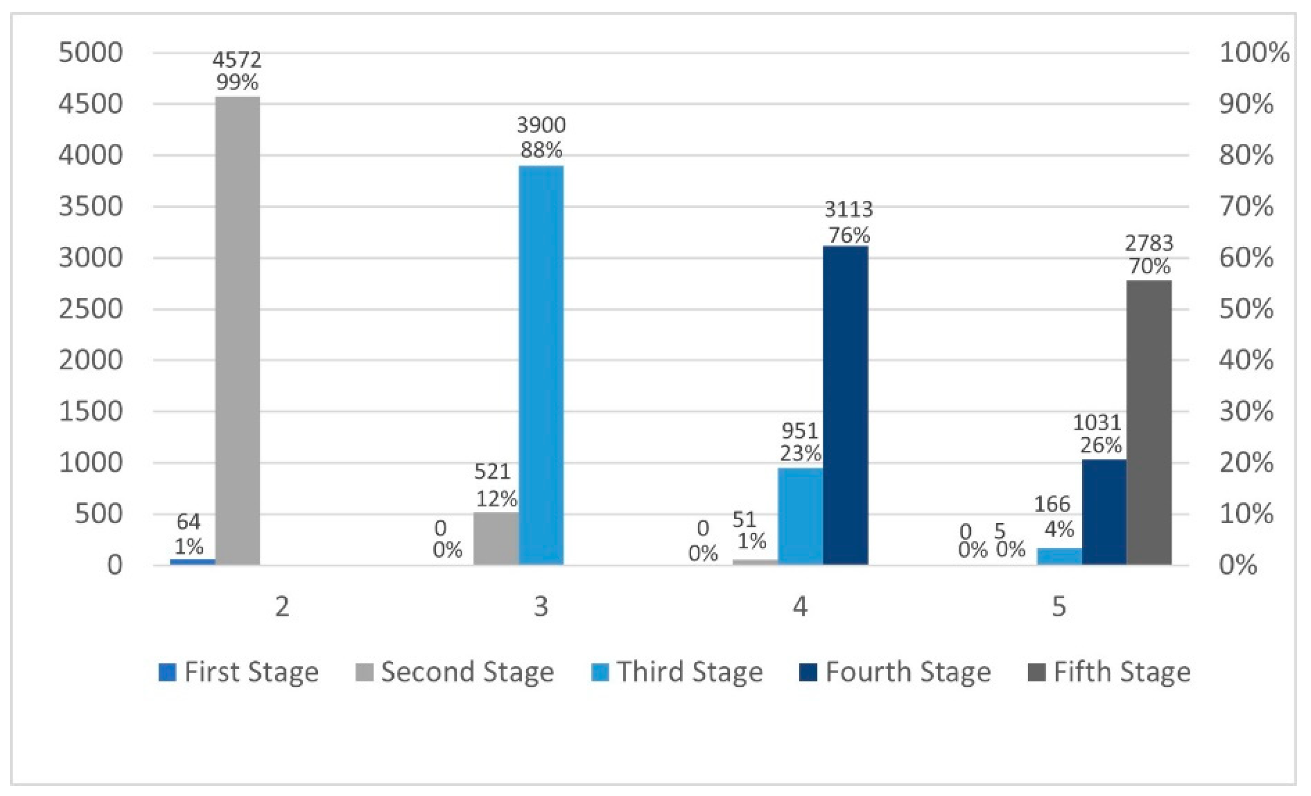
Table 8 and
Figure 7 below illustrate the required sample sizes and the number of rejections (percentages) at each stage for all values of
. It needs to be noted that these percentages are out of the 5% rejecting rate. The decision rules for this multiple-testing procedure are nearly identical to the usual chi-square one-stage procedure in the absence of early termination when
is true.
4. Examples
4.1. Example 1: Real Life Example
Three hundred individuals’ behavior was examined regarding their parents’ smoking status and how it influences their behavior. Participants were chosen based on their smoking status: 150 smokers and 150 non-smokers, then their parents’ smoking status were recorded. After assigning data for each value of from 1 to 5, OWMP was applied. The necessary sample size was also noted when the hypothesis was rejected. For illustrative purposes, both methods were applied when : the original O’Brien and Fleming method, as well as the OWMP.
Briefly, the procedure is explained for : , , , , and by using the weighted formula, we got: , , , .
For the first subsample: equal 60 because the subsample was divided equally. The chi-square statistic equals 1.534 after multiplying it by one fourth, which is not greater than the critical value of 4.0961, so we failed to reject .
For the second stage, with , and are needed to be recalculated by using the optimal allocation. Where with = .
The optimal allocation resulted in 42 and , with the chi-square statistic equal to 23.05, which is larger than the critical value after multiplying it by 2/4. Thus, is rejected.
Only two stages out of four stages, with only 196 out of the 300 participants, were needed to end the experiment and get a significant difference between the two treatments. In addition, using the original O’Brien and Fleming method, the following results were observed:
For the original procedure, equal subsamples are used as follows: 76
For the first stage, with , the chi-square statistic equals 0.163. Multiplying it by one-fourth resulted in a value that is not greater than the critical value of 4.096, so a significant difference was not found.
For the second stage, with , and the chi-square statistic for the cumulative data equals 5.856. Multiplying it by two-fourths resulted in a value that is not greater than the critical value, so a significant difference was not found again.
For the third stage, with , the chi-square statistic for the cumulative data equals 39.097. Multiplying it by third-fourth results in a value that is greater than the critical value, so a significant difference was found with using 228 participants in three stages, compared to 196 with two stages by using OWMP, which means OWMP reached the same conclusion with fewer stages and participants than the original procedure.
We can see a difference with only 180 patients, which is less than the 300 patients that would have been used in a conventional clinical trial.
4.2. Example 2: Computational Example
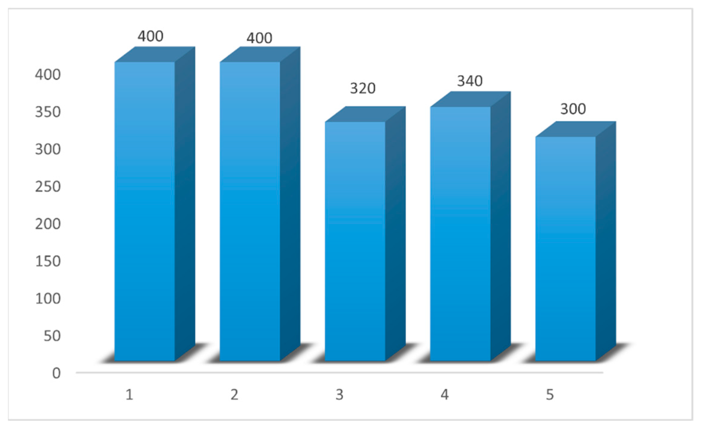
Simulated data of 400 subjects for two groups were used, with a success rate of 0.23 and 0.4 for group 1 and group 2, respectively (consequently, the alternative hypothesis is correct). Data from this trial were simulated, and the case when K equals three () was studied in detail, where = 45%, = 35%, = 20%, and by using the weighted formula, .
For the first subsample:, because the subsample was divided equally into the two groups in the first step. The chi-square statistic equals 0.88 after multiplying it by one-third. The result is not greater than the critical value of 4.02, so failed to be rejected.
For the second stage, with , and were calculated by using the optimal allocation. That resulted in 63 and . Moreover, the chi-square statistic equals 5.42, which is larger than the critical value after multiplying it by two thirds. Thus, was rejected, and a significant difference was found.
In this case, the trial is terminated using only two stages out of three stages, with only 320 of the 400 subjects needed to get a significant difference.
The remainder of the results are shown in
Table 9.
5. Discussion
Group sequential procedures based on multiple primary critical points are used as central cornerstones of strata tests to increase the efficiency of clinical trials. These multiple critical endpoints provide a complete characterization of the effect of any intervention in trials. Several of these procedures have been proposed. O’Brien and Fleming (1979) first proposed a proper multiple testing procedure. Its original critical points were modified for more accuracy and to exhibit a monotonic behavior with 1,000,000 iterations, by Hammouri [
15].
As a generalization, in this work, the O’Brien and Fleming procedure was combined with two different modifications for more fixable trials: the optimal allocation and unequal weighted allocation for subsamples. These two allocations were chosen since the optimal allocation implementation assigns more subjects to the more effective treatment. At the same time, the unequal weighted allocation allows for different subsample weights for different stages instead of equal allocation at each phase. Thus, it is possible to terminate the trial early and orient the largest number of participants toward the most effective treatment. The Type I error and power was calculated for several scenarios with several sample sizes to check the validity of this work. It was noticed that the new combination decreased the values of the Type I error and maintained the power in comparison with the usual chi-square, which indicates that OWMP is effective.
In detail, the Type I error values were computed with various values and sample sizes. The first case was with and the sample size equals . We noticed that the initial values for the Type I error with were between 0.0499 and 0.0503. The critical values monotonically decreased, whereas the number of increased, such that when the the Type I error values were between 0.0415 and 0.0438, which is less than 0.05, which means it is an acceptable error, and better than the error in the original procedures.
Moreover, with and the sample sizes equal to 80 and 580, the Type I error values were between 0.0418 and 0.0506, 0.0438 and 0.0507, respectively, which is acceptable since the values are not more than 0.0507.
Similarly, with the values of the Type I error values, in general, took on an analogous monotonic behavior, and the values were between and 0.0104. Again, the values decreased while the value increased, which is acceptable since the values are still not more than 0.0104. It is worth mentioning that the higher values occurred for , which represents the usual chi-square. Alternatively, all values were less than 0.05.
To determine whether the proposed procedure maintains the acceptance rate of the hypothesis when it is true (power), several comparisons were made with different values for success rates and sample sizes. The probability values were 0.1 with 0.15, 0.2, 0.25, and 0.3 with sample sizes 1366, 750, 200, and 120, for and 2032, 588, 292, and 182, for . The power results indicated that OWMP preserved the acceptance rate (power) despite the slightly decreasing values. The values decreased according to the division of the chi-square values by the number of stages in the interim analysis. This decrease in the chi-square values makes the rejection of harder. Nevertheless, values are still acceptable since the power values were between 0.8020 and 0.8164 for , and between 0.7726 and 0.7892 for . Thus, the difference between the values is not more than 0.044 for . In addition, for , the power values are acceptable since they remain between 0.8010 and 0.8113 for , and between 0.7840 and 0.7888 for . Thus, the difference between the values is not more than 0.0273.
Furthermore, the rejected iteration numbers and percentages were calculated under two scenarios of being true or false. Under being false, across the 500,000 samples, there was no significant difference between the OWMP and the usual chi-square test, and in the absence of early termination, the procedure’s decision rules are almost identical to those of the chi-square test. In contrast, when is true, the OWMP terminated the trial early in most cases, indicating that a smaller sample size is required to reject the hypothesis compared to the usual chi-square test.
The usual chi-square procedure collects data in much the same way as the O’Brien and Fleming multiple testing procedure and the proposed OWMP in this paper, but at once. Because the chances of a Type I error and power are basically the same for all procedures, the multiple testing procedures appear to gain nearly a considerable advantage over the usual chi-square procedure. Furthermore, the new OWMP is more flexible than the original multiple testing procedure. Researchers who would have otherwise adopted a single sampling design can now review their data periodically and terminate the study early if one treatment proves to be superior to the other, without sacrificing any of the advantages of sequential methods.
As a result, the OWMP proposed in this work is believed to be more effective than both the single sample approach and the O’Brien and Fleming multiple testing.
In our subsequent work, a plan was made to compare the OWMP performance to other previous procedures developed for testing binary outcomes, and to explore the possibility of generalizing other multiple testing procedures by combining different allocations to prechosen approaches [
27,
28,
29,
30,
31,
32,
33,
34]. We also plan to modify the original O’Brien and Fleming procedure by combining it with several new allocation methods. Furthermore, the proposed approach will be further expanded, by using the modification used for the O’Brien and Fleming original procedure, from two to ten treatments and the number of stages from five to ten by using more iterations to broaden our scope [
35].


