Abstract
For energy management systems, it is crucial to determine, in advance, the available energy from renewable sources to be dispatched in the next hours or days, in order to meet their generation and consumption goals. Predicting the photovoltaic power output strongly depends on accurate weather forecasting data and properly photovoltaic panel models. In this context, several traditional thermal models are expected to become obsolete due to the removal of the widely used Nominal Module Operating Temperature parameter, stated in the IEC 61215-2:2021 standard, according to reports of longer time periods in test data processing. The main contribution of the photovoltaic power estimation algorithm developed in this paper is the integration of an accurate procedure to calculate the hourly day-ahead power output of a photovoltaic plant, based on three simplified thermal models in steady state. These models are proposed and evaluated as remedial alternatives to the removal of the Nominal Module Operating Temperature parameter—a subject that has not been widely addressed in the related literature. The proposed estimation algorithm converts specific Numerical Weather Prediction data and solar module specifications into photovoltaic power output, which can be used in energy management applications to provide economic and ecological benefits. This approach focuses on rooftop-mounted mono-crystalline silicon photovoltaic panel arrays and incorporates a nonlinear translation of Standard Test Conditions parameters to real operating conditions. All necessary input data are provided for the analysis, and the accuracy of experimental results is validated using appropriate error metrics.
1. Introduction
Solar energy is a promising renewable energy source capable of driving the world’s current and future energy consumption needs [1]. It has received special attention due to the ongoing depletion of fossil fuels and their negative environmental impact. Over 40 countries, including Mexico, have pledged to tackle the climate crisis associated with polluting energy sources and achieving Net-Zero emissions by 2050 or shortly thereafter [2]. As a competitive solution to this scenario, solar energy has proven to be both abundant and environmentally friendly. In recent years, solar photovoltaics have experienced a remarkable boom in developing and developed countries. The solar photovoltaics market achieved its largest annual capacity increase ever recorded, reaching 407 Giga-Watts (GW) in 2023, and bringing the global cumulative solar photovoltaic (PV) power capacity to 1589 GW by the same year [1].
Positive increases in the penetration of distributed PV generation can also become problematic when considering the inherent uncertainty of variable weather conditions. High variability in solar energy generation has been associated with grid disruptions and shortages [3]. On sunny days, high PV power generation can meet the consumers’ internal demand and produce significant surplus energy to supply the power grid. Conversely, on cloudy or rainy days, power generation may fall short of expected targets, negatively impacting continuity and reliability quality parameters.
As a viable alternative to mitigate the negative impacts of Variable Renewable Energy (VRE), Energy Management Systems (EMSs) can optimize generation and consumption during energy surplus and shortage conditions. Economic benefits can be achieved by reducing financial losses caused by energy imbalances and improper energy dispatching. Optimization strategies prioritize the dispatch of renewable energy, resulting in ecological benefits such as minimizing dependence on fossil fuels, lowering carbon footprints, and reducing greenhouse gas emissions. To realize these benefits, energy management strategies require accurate power forecasting models to estimate, in advance, the available energy from renewable sources, for the next few hours or days.
Several methods in the literature employ PV power estimators based on historical weather records to perform short-term forecasting. Statistical models have been widely used as simple tools that establish correlations between meteorological input variables and PV power output. However, they often overlook future atmospheric conditions, which negatively affects their accuracy. In contrast, machine learning algorithms have become the most widely adopted approach for PV power estimation in recent studies, due to their ability to capture the dynamic and variable nature of environmental conditions. These models typically rely on historical data but can also incorporate weather predictions, thereby improving their reliability and accuracy. In addition, many power estimation methods incorporate physical equations to transform meteorological inputs into power output. However, some of these approaches might depend on detailed PV panel models requiring parameters and specifications rarely provided by manufacturers, making them impractical for real applications.
Weather Prediction Data (WPD) has become a critical component in PV power estimation. Among the most commonly used sources for WPD are Numerical Weather Prediction (NWP) systems. NWP are widely adopted due to their capability to simulate atmospheric dynamics with high spatial and temporal resolution. By integrating satellite imagery and infrared observations, these systems provide accurate forecasts suitable for PV power estimation.
The overall performance of PV power plants is significantly affected by various factors such as shading, module degradation, and variable conditions of humidity, wind speed, irradiance, and temperature, among others. Shading losses—caused by shadows from trees and buildings, dust accumulation and manufacturing imperfections—and power degradation over the PV panels’ lifetime are major contributors to reduced power capacity. However, accounting for all these factors considerably increases the complexity of system modeling. Considering common operating practices and panel specifications—such as PV mounting installations located away from trees and buildings, regular cleaning maintenance, and the use of new solar modules—can significantly simplify PV power models. Accordingly, the estimation methodology proposed in this paper focuses on the most significant effects resulting from variations in irradiance and temperature, in order to incorporate a simplified PV model.
As the PV panels efficiency strongly depends on the module temperature, one of the most commonly used parameters in traditional PV models is the Nominal Module Operating Temperature (NMOT). This parameter was introduced in the IEC 61215-2:2016 standard as an update to the Nominal Operating Cell Temperature (NOCT), to estimate the temperature of PV modules under certain local environmental conditions of solar irradiance, ambient temperature, wind speed, and so on [4]. However, Section A.11 of the IEC 61215-1:2021 standard [5] describes the removal of NMOT, according to reports of longer time periods in test data processing. Since no replacement parameter is proposed in the standard, new PV models require alternative methods to determine the module temperature without relying on NMOT.
In this paper, a PV power estimation algorithm is proposed to determine the hourly day-ahead power output of a PV plant. The algorithm integrates accurate local weather prediction data from NWP systems with simplified thermal models in steady state. Three simplified PV thermal models are proposed and evaluated as remedial alternatives to the removal of the NMOT parameter, filling the gap in the recent literature on PV power estimation models in this context.
The PV power model employed in this work incorporates parameters and specifications under Standard Test Conditions (STCs), which are commonly provided by PV panel manufacturers, and applies appropriate mathematical translations to convert them to non-standard operating conditions. A validated case study is presented, focusing exclusively on monocrystalline PV module technology, which accounted for nearly 98% of the PV module market in 2024 [6]. Furthermore, a sloped rooftop-mounting configuration is considered, as it represented the largest share of solar PV installations in 2023 [1].
The proposed PV power estimation algorithm is used by an EMS—not described in this work—to mitigate the variable effects of PV generation, for an industrial consumer in Mexico, where the hourly estimation of the day-ahead PV power capacity is essential.
2. Solar Power Forecasting
PV power generation strongly depends on solar irradiance and ambient temperature, which are influenced by variable weather conditions. Solar power forecasting, based on weather predictions at specific site locations, has proven to be an essential source of information for numerous planning processes within the energy industry. Furthermore, it serves as an effective tool for integrating VRE resources, such as PV solar, into power systems [7,8,9].
2.1. Numerical Weather Predictors
Solar power prediction systems typically rely on numerical weather models, as these are uniquely capable of simulating atmospheric behavior in the near future. Consequently, NWP models are the physical models most commonly used in weather forecasting applications [7,10]. NWP models divide the atmosphere into grid cells, with sizes ranging from a few hundred meters to twenty km, and calculate the meteorological average parameters for each cell. Commercial weather forecasting services achieve greater accuracy by employing weighted combinations of multiple NWP models, each specializing in specific weather conditions such as storms, high-pressure fronts, morning fog, and etc. Pure statistical methods, based on historical records and observed values, are also used in solar power prediction. They perform best for the intra-hour time horizon (shortest-term forecasts), but may have some value out from time scales extending beyond two to three hours [9].
In the proposed estimation algorithm, local Weather Prediction Data (WPD) of solar irradiation and ambient temperature are provided by commercial weather forecast services, such as those offered in [11,12]. These commercial providers incorporate specialized NWP technologies, based on visible and infrared channel data captured by geosynchronous orbiting satellites, positioned all around the world to provide hour and intra-hour weather forecasting resolutions in the short- and shortest-term horizons, respectively. This is why such commercial WPD systems can achieve hourly accuracy metrics for Global Horizontal Irradiance (GHI) around rMAE values from 10% to 12%, depending on the forecasting global area.
2.2. Time Horizons
Distinct time scales for forecasting are used to predict the power capacity that PV modules will generate over the coming hours or days. The most common time horizons are listed below:
- Shortest-term forecasting (1 min to 6 h ahead): Essential for intraday energy market trading, power regulation, balancing, dispatch, and curtailment operations.
- Short-term forecasting (6 to 48 h ahead): Applied in day-ahead energy market trading, power regulation markets, load flow calculations, and PV-integrated energy management systems.
- Medium-term forecasting (2 to 20 days ahead): Typically used for trading energy markets, congestion management, and maintenance planning.
- Long-term forecasting (Weeks, months, seasonal and years ahead): Useful for power unit commitment, generation, transmission and distribution management, trading, hedging, planning and resource optimization, and investment planning of PV projects.
A general principle to consider is that forecasting accuracy decreases as the look-ahead time increases [8,9,13,14]. Consequently, the proposed methodology focuses on short-term forecasting to estimate the PV power output for the next 24 h.
2.3. Conversion of Weather Prediction into Solar Power Forecasting
There are three prevalent methods for converting meteorological data into power forecasts: statistical, physical, and hybrid approaches [14,15,16,17].
- Statistical methods utilize historical and real-time power generation data, along with NWP data, to “train” predictive models using machine learning algorithms such as artificial neural networks, regression models, autoregressive models, support vector machines, and Markov chains, among others.
- Physical methods use specific weather data inputs (e.g., from NWP) and directly convert them into PV power output through PV panel models.
- Hybrid methods combine statistical and physical approaches to achieve higher accuracy in cases where sufficient weather data are available.
As a common practice, PV power generation data is often recorded by measurement systems at the plant location. However, specific local historical weather data may not be available. Consequently, in cases where such data is insufficient or unavailable, the proposed estimation methodology applies a physical forecasting scheme based on specific NWP data points—such as Diffuse Horizontal Irradiance (DHI), Direct Normal Irradiance (DNI), albedo, wind speed, and ambient temperature—to model and convert WPD into PV power output.
3. PV Power Estimating Models in Literature
As an essential part of EMS, various PV power forecasting models have been developed and adopted in recent literature. VRE forecasting is widely used in electric system operations, such as dispatch, real-time balancing, and reserve requirements, to cost-effectively balance load and generation in intra-day and day-ahead scheduling. This leads to reduced fuel costs, improved system reliability, and minimized curtailment of renewable resources [8]. Reducing fossil fuel consumption, along with implementing energy efficiency measures, not only generates financial savings but also promotes emissions reductions and carbon dioxide removal, thereby mitigating environmental impact [2].
The most recent, popular and heterogeneous methodologies for PV power forecasting can be classified according to their underlying architectural method or mathematical structure into statistical, machine learning, physical, and hybrid models [17].
3.1. Statistical Models
Statistical models utilize the historical data of dependent variables (e.g., solar irradiance, ambient temperature) to identify the correlation between input variables and PV power output. These models often incorporate additional information derived from independent variables (e.g., day of the week, hour of the day, month number), commonly referred to as exogenous variables. Time series of historical data are analyzed using Autoregressive (AR), Integrated (I), and Moving Average (MA) algorithms, which together form the basis of some of the simplest forecasting models, such as ARMA and ARIMA models [10]. Statistical models are generally simple, computationally efficient, and effective for very short-term forecasting [17]. However, they are highly sensitive to missing or incomplete data and often fail to accurately represent nonlinear relationships between dependent variables [10].
As mentioned in Section 2.1, some limited PV power estimators use weather prediction methods for forecasting PV power output based solely on historical data, which consists of past weather samples and measurements (without considering WPD). This is the case in [18], where statistical methods for weather prediction might exhibit a poor performance in the short-term. Similarly, in [19], a day-ahead forecasting of solar irradiance and temperature based on historical and target data is performed using a Multilayer Perceptron Neural Network (MLPNN). At these time scales, accurate forecasting models should combine predicted weather conditions with historical data [7].
3.2. Machine Learning Models
Machine Learning (ML)-based models are the most widely adopted for PV power estimation in literature [14], mainly due to their high accuracy in short-term forecasting horizons [10]. Their popularity stems from their ability to effectively capture the highly nonlinear relationships between environmental input variables and PV power output [14].
These models extract relevant information using training algorithms that establish mathematical relationships between historical solar generation data and meteorological conditions. ML algorithms that rely on labeled datasets with known input–output pairs are referred to as supervised learning algorithms. Examples include regression algorithms, Artificial Neural Networks (ANNs), Support Vector Machines (SVMs), and k-Nearest Neighbors (k-NNs), among others. In contrast, unsupervised learning algorithms do not require labeled outputs and are used to discover hidden structures in the data. Common unsupervised methods include k-means clustering, hierarchical clustering, ensemble methods, boosting, bagging, and decision trees [10].
Deep Learning (DL) models represent a specialized subclass of ML algorithms, which can be either supervised or unsupervised. These models are composed of advanced neural networks with multiple layers and memory units, allowing them to extract deep and specific features from dependent variables [14]. The DL models most commonly used for PV power forecasting include Convolutional Neural Networks (CNNs) and Long Short-Term Memory (LSTM) networks [14]. In general, the performance of ML algorithms is highly dependent on the quality and availability of the training data, as well as on significant weather variations over short timeframes [10]. Historical input datasets often contain a significant number of outliers, noise, or missing values, which can substantially degrade forecast accuracy. For this reason, pre-processing methods are critical to enhancing the performance of ML models [16]. Moreover, establishing a robust relationship between input and output variables requires appropriate training parameters and, in some cases, feature selection or refinement based on relevant criteria [10].
3.3. Physical Models
Physical models for PV power systems use site-specific information, detailed climate parameters, panel orientation, and module-specific parameters and specifications to develop mathematical equations for determining the output power of a solar array. When based solely on solar irradiance analysis, these models remain relatively simple; however, their complexity increases significantly when additional parameters—such as ambient temperature and wind speed—are considered [15]. Unlike statistical models, physical models do not rely on historical data to estimate PV power output. Instead, they incorporate physical specifications of the PV array along with weather forecast data, typically obtained from Numerical Weather Prediction (NWP) systems. This makes them highly efficient for short-term forecasting applications [16].
In the present work, a physical model is adopted that utilizes specific weather-dependent parameters (WDPs), along with PV module specifications provided by manufacturers, to estimate the power output of a solar array. Some applied physical models from literature are included and described in Section 3.5.
3.4. Hybrid Models
Hybrid models are structured combinations of statistical, machine learning, and physical approaches that have gained considerable attention in PV power forecasting due to their ability to leverage the strengths of individual models and capture diverse patterns in the data. These models can be integrated either sequentially or in parallel, depending on the adopted forecasting architecture [17]. In a sequential configuration, the output of one model is the input to the subsequent model. In contrast, parallel configurations utilize individual models operating independently, whose corresponding outputs are weighted and integrated to produce the final forecasting result [20]. Some of the hybrid models commonly reported in the literature include the following: Physical–Statistical Hybrid Models: These approaches combine physical formulations to represent PV system parameters with statistical techniques that capture data variability and enhance modeling flexibility. Physical–Machine Learning Hybrid Models: In addition to the precision of physical modeling, the integration of machine learning techniques—such as ANN, SVM, and CNN—allows these models to effectively capture complex dynamics, nonlinear relationships, and uncertainties associated with PV power generation [17]. In most scenarios, hybrid models tend to outperform the individual models they incorporate. Nevertheless, similar to standalone machine learning approaches, their performance is highly dependent on the quality and quantity of the training dataset. Consequently, in cases with limited historical data, optimized physical models are often more suitable and reliable [20].
3.5. Applications of Physical Modes in Literature
Several physical PV panel models in energy management applications assume a linear relationship between the maximum PV power output capacity and the solar irradiance on the PV panel surface. Such is the case in [21], where a power estimation model describes a simple linear relation between PV power output and the global irradiance on the PV panel surface. The same linear model is used in [22] to calculate the PV power output of a hybrid renewable power system, including the temperature coefficient and the de-rating factor. A similar case is proposed in [23], where the called Ostwald’s technique is used to estimate the PV power output by mean of a linear contribution of the total irradiance on the PV panel surface. In [24,25] the ratio of the total irradiance on the PV panels and the STC irradiance value is used to determine the PV power output. Additionally, a simple PV generation model, based on a linear relationship between solar irradiance, panel efficiency, and photovoltaic area, is employed in [26] to estimate the power exchange of a grid-connected PV plant. However, under real operating conditions, solar irradiance and PV power output are the subjects of nonlinear behavior [10]. According to the exhaustive analyses presented in [27,28], as well as certified irradiance performance data of PV modules under STC conditions from manufacturers (e.g., REC panel modules [29]), the output capacity of PV panels exhibits a logarithmic dependence on solar irradiance, with a particularly pronounced effect under low-irradiance conditions (i.e., 1–300 W/m2). Therefore, linear approximation models lead to significant errors in PV power estimation and prediction processes.
In addition, thermal PV models are typically used in combination with solar irradiance models to describe the dependence of PV power output on module temperature. In this context, one of the most commonly used parameters for estimating PV module temperature is the NOCT parameter, the predecessor of NMOT [30]. Authors in [25,31] use this parameter in thermal models to determine the PV module’s temperature under operating environmental conditions. Although NMOT is still included as a useful parameter in manufacturers’ datasheets (e.g., Qcells Panel Modules [32])—primarily due to its compatibility with traditional thermal models and existing simulation tools, and due to industry inertia—it is expected to become obsolete following its removal from current industry standards.
Furthermore, energy management strategies and optimized PV power estimation methods—such as the one described in [33]—consider that the parameters from diode-equivalent models of PV modules exhibit a significant nonlinear relationship with power output. Therefore, these parameters must be previously transformed to allow finer and more accurate estimation performance. A similar circuit equivalent model, based on electric parameters and specifications, is described in [34] to improve the grid-connected stability of PV power plants. Nevertheless, certain parameters—such as the cell voltage , diode voltage , and the series and shunt resistances, and —are rarely provided by manufacturers of PV modules, making these models impractical for real applications.
As can be seen, the reviewed literature reveals several areas of opportunity in PV power estimation modeling. In this paper, the proposed algorithm focuses on integrating a proper procedure to estimate PV power output based on the nonlinear relationship between widely available STC parameters of PV panels and predicted solar irradiance. Additionally, a physical method, without the requirement for historical weather records, is adopted to convert WPD from commercial NWP into day-ahead PV power output forecasting, performing adequately in the short term. Furthermore, three alternative thermal models are proposed and validated to mitigate the negative impacts associated with the removal of NMOT from commonly used standard parameters.
4. PV Panel Thermal Models
PV panel efficiency is highly dependent on the cell operating temperature. Under real operating conditions, high incident irradiance levels cause PV cell temperature increases, which significantly affect its overall performance [31,35]. Thereby, predicting the PV power output requires appropriate thermal models of solar panels to estimate the cell/module operating temperature (), based on local environmental conditions such as solar irradiance, ambient temperature, wind speed, and more [35,36].
Thermal models used to estimate can be classified into two main approaches: steady state and transient/dynamic state. In the steady state, simplified thermal models consider the intensity of the incoming solar irradiance, and other parameters affecting the performance of PV modules, as constant in the short period of time. Otherwise, such parameters are assumed to be time-dependent in the transient or dynamic state. In this case, complex models, performing differential equations, are more realistic and accurate in their estimation of , under rapid fluctuations of solar irradiance, in the shortest period of time [31,35]. As dynamic approaches usually require a longer computation time and specific module parameters (e.g., transmittance and absorbance), which are rarely provided by manufacturers of solar panels, only simplified thermal models in the steady state are considered in this paper.
In steady state, the energy balance of a PV module unit can be written as follows:
where and are the module/cell nominal efficiency and the total irradiance on the PV panel surface, respectively. and a are the transmittance and the absorptance of the module cover and PV layers, and are the module/cell and the ambient temperatures, and is the thermal loss coefficient (W/m2°C) [37]. From (1), several PV thermal models can be derived to determine under specific operating conditions; such is the case with model in Section 4.1.
4.1. The Nominal Module Operating Temperature (NMOT)
Traditional thermal models have been successfully applied to PV cells and modules to determine based on their nominal operating conditions. Such is the case with (2), proposed in [25,30,31] as a common method to determine , by considering the NMOT parameter defined in the IEC 61215-2:2016 standard and widely provided in most datasheets of PV panels. NMOT is the replacement for the former Nominal Operating Cell Temperature (NOCT) [4].
When usual assumptions of constant and smaller (/()) compared to unity are made [37], and the Nominal Terrestrial Environment (NTE) conditions (i.e., solar irradiance 800 W/m2, ambient temperature 20 °C, wind speed () 1 m/s) are considered, (1) can be simplified as follows:
NMOT describes the performance of a module/cell under NTE conditions [4]. Therefore, the operating module temperature for installed PV panels is defined as (3).
Here, = + m, is the Installed panel mounting NMOT. The mounting term m is °C for direct mounting and °C for rack mounting PV panels. For standoff mounting at heights of 1, 3, and 6 inches, m is °C, °C and °C, respectively [38].
The NMOT procedure described in [4] is based on the determination of the heat loss coefficients and defined in the Faiman Model [39] to calculate the module temperature. Nevertheless, reports of strict data filtering taking unacceptable periods of time led the project department of the International Electrotechnical Commission to definitely remove the NMOT test from the current IEC 61215-2:2021 [40]. Such decision urges and promotes designers of PV systems to consider alternative thermal models to determine the module operating temperature and, consequently, the power output estimation of PV panels.
Actually, the NMOT parameter is still included and issued in most of the datasheet specifications of recent PV panels around the world and still used in practice, but is expected to be withdrawn in the near future.
To solve the inconvenience of the NMOT removal, three additional thermal models are proposed and validated in this paper, as proper alternative methods to calculate the module operating temperature. These are the Ross model, the Sandia model, and the Skoplaki model.
4.2. The Ross Model
A simple and widely used model is described in the explicit Equation (4) proposed by R.G. Ross [41], as a linear expression in terms of , the Ross coefficient k, and to determine .
Here, the slope k is the ratio of the temperature rise above the ambient temperature () to the increasing irradiance () [37], with values in the range of 0.02–0.055 °C m2/W, with °C m2/W being the most broadly accepted value [42]. The Ross coefficient, k, depends on the type PV module, the mounting installation, and the cavity on the back of the module [43]. Table 1 shows the experimental values of k, according to the mounting installation of PV panels [37].

Table 1.
The Ross coefficient, k, for various PV mounting configurations.
4.3. The Sandia Model
The Sandia thermal model (5), created by the Sandia National Laboratory in the United States, is a simple method for determining based on empirical coefficients influenced by the PV panel construction, the mounting installation, and the wind speed at the specific location [36]. The model’s performance has been successfully applied to PV panels in open-rack, insulated-back, and close-to-roof mounting installation schemes, and proved to be an accurate method for wide engineering applications.
where a describes the upper limit for at low wind speeds and high solar irradiance and b is the rate at which drops as wind speed increases. is the wind speed (m/s) at standard 10 m height. Both empirical coefficients are obtained in near thermal equilibrium conditions (i.e., nominal clear sky conditions without temperature transients due to intermittent cloud cover) [36].
Measured data registers under near thermal equilibrium conditions of solar irradiance, wind speed, and wind direction, recorded over several days for a determined PV panel, in a particular mounting configuration, are fitted by a linear regression process to provide the coefficients a and b in (5). Table 2 shows some empirical coefficients used by the Sandia thermal model for two types of PV panels (Glass/cell/glass and glass/cell/polymer) and three types of mounting installation schemes [36].
Table 2.
Empirical coefficients for the Sandia thermal model.
4.4. The Skoplaki Model
The module temperature can be determined by considering some empirical correlations with the energy balance of a PV panel and the individual components of its thermal loss coefficient (). In the Skoplaki model, typical specifications of PV modules under NTE conditions, provided by manufacturers, are substituted in (1) to lead the general expression for the operating temperature (7), based only on the forced convection component of , where expected error of ignoring free convection and radiation losses is assumed to be minor [37]. The linear correlation of the wind convection coefficient, , proposed by D.L. Loveday [44], is considered as the forced component of .
Here, is the free local wind speed (m/s), well above the PV array (e.g., standard 10 m height).
Equation (7) is suitable for free-standing arrays, but can be modified to perform in other PV panel mounting configurations by means of the mounting coefficient, . Table 3 shows different values of , according to the PV array mounting configuration [37]. Therefore, the module temperature, for wind speeds (m/s), can be determined by the Skoplaki Model in (8), in terms of the three basic environmental variables and the correspondent mounting configuration scheme [37].
Table 3.
The mounting coefficient , for various PV panel mounting configurations.
5. PV Power Model
The PV power capacity of solar panels is usually expressed in terms of their Maximum Power Point () to describe the maximum power output of a PV module at STC. The STC for irradiance and cell temperature are 1000 W/m2 and °C, respectively [40]. is included in datasheets from PV panel manufacturers and can be obtained by various means (9) [27,45].
Here, and are the open-circuit voltage and the short-circuit current at STC. is the Fill Factor.
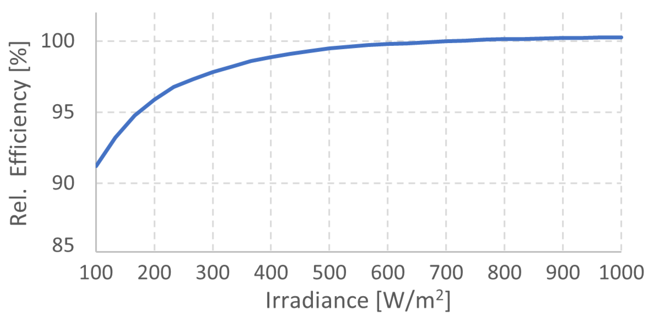
As mentioned in Section 2, PV power capacity is highly influenced by variable conditions of irradiance and temperature; hence, STC parameters must be translated into real operating conditions. The translation Equations (10) and (11) [28] are used in this paper to ensure the adequacy of the PV panel parameters at STC, to variable irradiance levels, at an initial invariable module temperature of 25 °C. Here, holds a linear relationship with , in contrast with , which exhibits a logarithmic dependence to solar irradiance.
and are the open-circuit voltage and the short-circuit current under variable irradiance levels, at invariable module temperature of 25 °C. The irradiance correction factor of the open-circuit voltage, , is inherently dimensionless and obtained from the I–V curves of the corresponding PV technology. Most common values of are 0.085 for m-Si, 0.11 for p-Si, and 0.063 for a-Si [28]. The logarithmic dependence of in (10) is clearly depicted in typical relative efficiency curves at STC, as shown Figure 1 [29].

Figure 1.
Typical efficiency performance of PV module at STC.
Therefore, (9) can be rewritten in terms of (10) and (11), for variable irradiance and standard module temperature of 25 °C, as follows:
The PV power model in (12) is used in Section 6.3 to determine the PV module efficiency under variable conditions of irradiance and temperature.
6. PV Power Estimation Algorithm
In this section, a simple procedure to estimate the PV power output capacity based on the thermal and power models described in Section 4 and Section 5, is proposed. The weather prediction data, at the PV array location, are used to determine both, the total solar irradiance on the panel surface and the module temperature, in the short-term horizon. Widely available STC parameters, provided by solar panel manufacturers, are properly translated to real operating conditions to calculate the panel efficiency and the PV power output.
6.1. Solar Irradiance on the PV Panel Surface
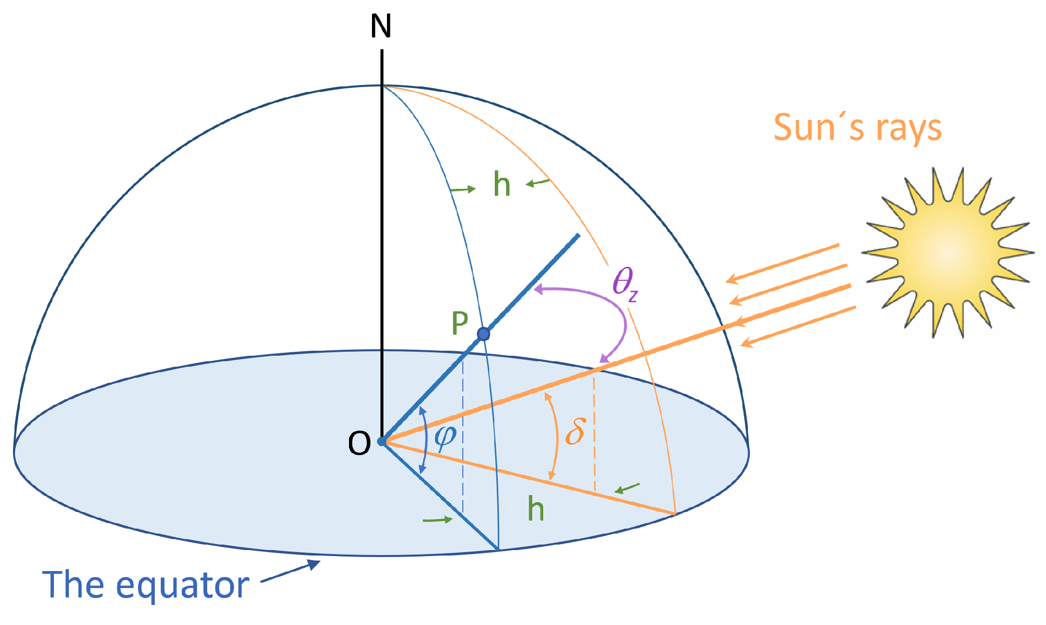
Estimation of PV power generation requires accurate prediction values of irradiance and ambient temperature at the plant location. As the sun is the principal source of irradiation in the world, it is crucial to determine the effective solar irradiance on the PV panel surface, . This value can be deduced from the GHI on the Earth’s surface in (13) and its DHI and DNI components [46]; frequently used in solar energy applications.
The solar zenith angle , is the angular difference between the vertical of the location plane (i.e., normal to earth) and the sun’s rays, as shown in Figure 2.
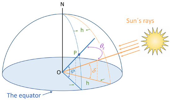
Figure 2.
Solar irradiation angles.
The Beam Horizontal Irradiance () can be deduced from (13) as follows:
Most PV panels in solar plants are mounted on tilted racks. Hence, the total irradiance, , is a fraction of corresponded on the Earth surface. The Liu and Jordan model, for isotropic diffuse sky condition, is used to determine based on three components: beam, diffuse, and global irradiance [47].
The beam solar irradiance on the PV panel surface, , is a portion of .
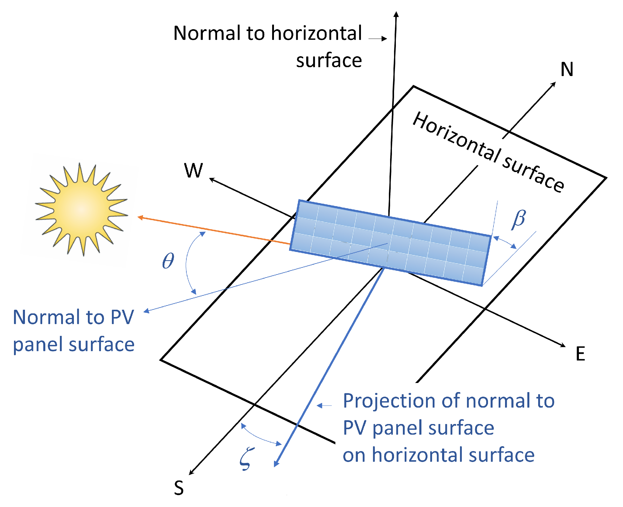
The angle of incidence, , is the angle between the normal PV panel surface and the sun’s rays, as shown in Figure 3. It is geometrically determined by the direction toward the sun at local latitude , considering the declination angle, , and the hour angle, h, as well as the PV array orientation expressed in terms of the panel tilt angle, , and the azimuth angle, [21,48].

Figure 3.
PV panel azimuth angle.
The azimuth is the angle between the projection of normal to PV panel surface to horizontal surface and the true south (westward is considered as positive, as shown in Figure 3). Both the panel tilt and azimuth angles are specific values of a particular PV plant.
For the PV plant, denotes the angle between the normal to the location plane and the sun’s rays. The cosine of can be obtained by (18).
As shown, when the PV panel surface is a horizontal plane (i.e., ), .
is the diffused solar irradiance on the PV panel surface, seen from the tilted module.
The last term in (15), the ground-reflected irradiance, , depends on the module tilt and ground reflectivity, .
The typical albedo or ground reflectivity values are 0.1–0.3, except on white surfaces (snow-covered), where reflectivities are closer to 1 [46].
6.2. Module Temperature
As mentioned in Section 4, PV panel efficiency is highly affected by the module temperature, . Traditional thermal models in the steady state have successfully used the NOCT and NMOT parameters, in STC, to determine . Due to the removal of these parameters from international standards, three alternative thermal models, based on local environmental conditions of solar irradiance, ambient temperature and wind speed, are considered in this paper. Table 4 shows a brief summary of the INMOT model (in transition), the Ross model, the Sandia model, and the Skoplaki model, described in Section 4, as alternative methods to determine the module operating temperature.
Table 4.
Thermal models for PV module operating temperature.
6.3. PV Panel Efficiency
The overall PV panel efficiency, in (22), is used to express the radio of useful work performed by a PV module to the solar irradiance, I, on its aperture surface, under STC [27,45].
Here, is the PV aperture area of a single module, or the total active area in a PV array.
Equation (22) is expressed in terms of the PV power in (12) to obtain the efficiency under variable irradiance levels, at an invariable module temperature of 25 °C, :
The PV module efficiency at variable levels of irradiance and temperature, , is obtained by (24) [49].
The temperature coefficient of , , is provided in datasheets by PV panel manufacturers.
6.4. PV Power Output
Finally, the direct current power output of a PV module or an entire array, considering nonstandard operating conditions of irradiance and temperature, can be estimated by (25).
In order to extend the proposed analysis to both alternating and direct current electric systems, as well as grid connected or isolated applications, the PV power output calculation in (25) does not involve power losses of power converters and Balance of System (BOS) equipment.
6.5. Proposed Algorithm
The PV power estimation algorithm proposed in this paper can be summarized as follows:
▹Step 1. The PV panel parameters and specifications on STC, such as , , , NMOT(°C), and (°), must be provided as input data from the manufacturers’ datasheet.
▹Step 2. The Global position angles of the PV panel array related to the sun’s rays, , , h, , and , shown in Figure 2 and Figure 3, and described in Section 6.1, must be provided as hourly input data for the entire time horizon (e.g., 24 h), on a specific day of the year.
▹Step 3. For fixed–tilted PV panels, it is necessary to determine the and by means of (17), or simplified (21) for south-facing PV modules, and (18), respectively.
▹Step 4. Determining the total solar irradiance on the PV panel surface, by means of (15) and its components (16), (19) and (20), using hourly , and , from WPD described in Section 2.1.
▹Step 5. Determining the module temperature, , by using one of the four PV thermal models proposed in Section 4, with obtained in Step 4, , or from WPD, and the properly mounting term.
▹Step 6. PV panel efficiency in (24) must be determined by means of the efficiency and power terms at invariable temperature in (23) and (12), as well as the translation Equations (10) and (11) and , , according to the PV panel technology.
▹Step 7. Finally, the PV power output estimation can be calculated by means of (25).
Steps 3–7 must be executed for each hour in the adopted prediction time, in order to fulfill the PV power estimation horizon.
A specific case study is analyzed to assess the performance of the proposed estimation algorithm.
7. Case Study
The PV power plant in the current analysis, from which the observed values originate, consists of 30 units of REC360NP2-Black Mono C-Si n-type solar panels, arranged in a sloped roof-mounted rack, facing south and tilted at 19.7°. The specific values corresponding to this configuration are m = −3 °C for the mounting term in the NMOT model described in Section 4.1, according to the rack mounting installation; k = 0.025 °C m2/W for the Ross coefficient defined in Section 4.2; a = −3.56 and b = −0.0750 for the Sandia Model in Section 4.3, according to the open rack category in Table 2; and = 1 for the mounting coefficient related to the Skoplaki model in Section 4.4, according to the sloped roof category in Table 3. The PV plant is located in Mich, Mexico, where = 19.7°. The relevant PV panel parameters under STC from datasheet are = 360 W, = 10.62 A, = 33.9 V, = 11.3 A, = 40.8 V, NMOT = 44.3 °C, = 19.7%, = 1.82 m2, °C−1 [29]. Table 5 shows a sample of the day-ahead WPD from commercial forecast service, corresponded to the 87th day of the year 2024.
Table 5.
Day-ahead WPD from commercial service.
8. Results
The proposed PV power estimation algorithm, summarized in Section 6.5, was applied daily during the case study and registered from March to September of 2024. PV thermal and power models in Section 4 and Section 5 are evaluated to compare their performance and accuracy. Estimated and observed PV power values are used in this section to provide daily, weekly, and monthly validation for the mentioned evaluation time. Corresponding validation metrics are described in the Appendix A.
Daily WPDs are considered to determine the hourly day-ahead prediction values of total irradiance on the PV panel surface, , and the PV power output (), for each of the proposed thermal models in Section 4. Table 6 shows an example of the day-ahead estimation outcomes corresponding to the case study and the WPD in Table 5.
Table 6.
Day ahead total irradiance and PV power output estimation outcomes.
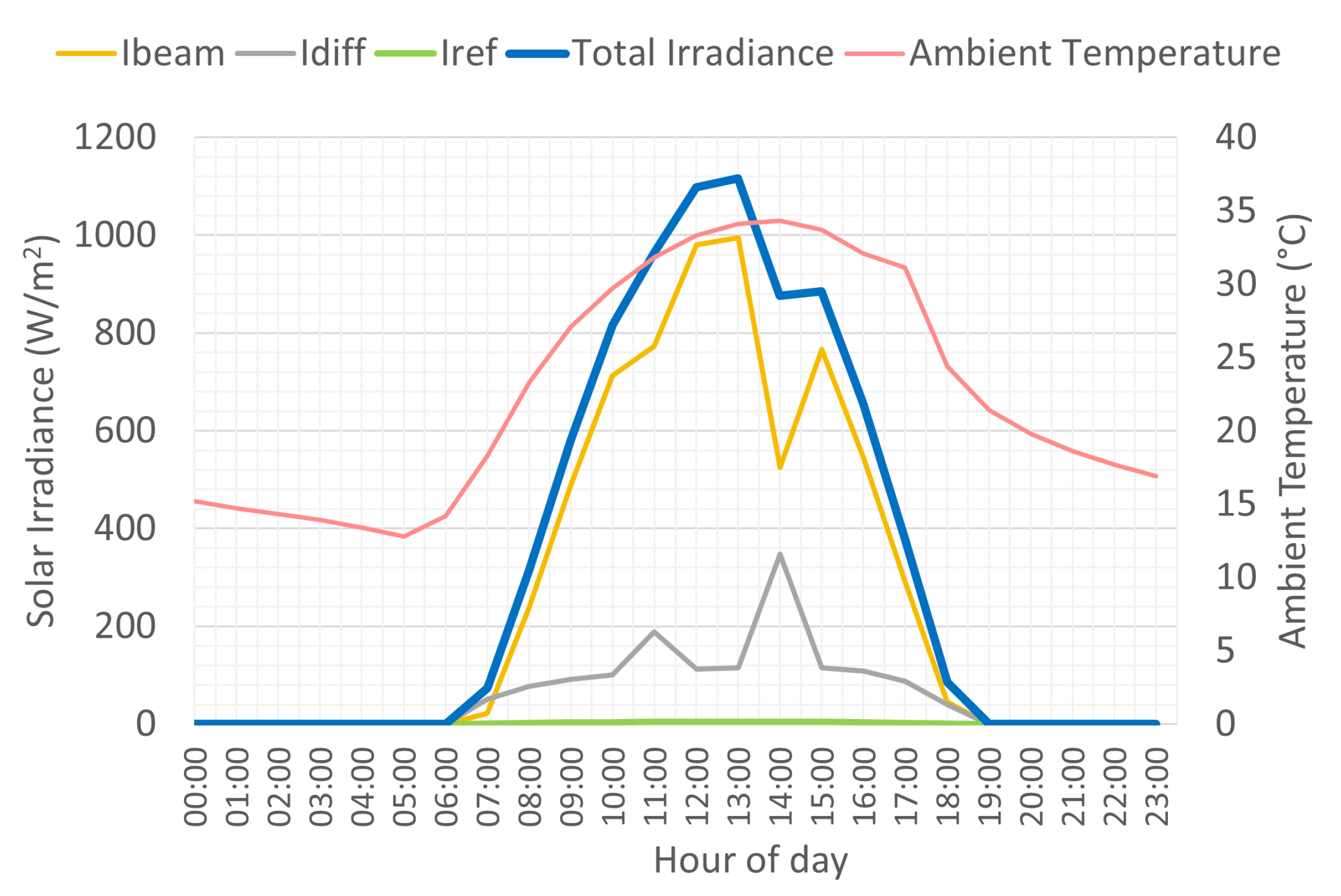
Figure 4 depicts the total irradiance, , and its components , , and described in (15). The ambient temperature, from Table 5, is also included in the graph. Here, the highest levels of total irradiance and ambient temperature are predicted between 11:00 and 15:00 hours.

Figure 4.
Total irradiance on PV panel surface, irradiance components and ambient temperature.
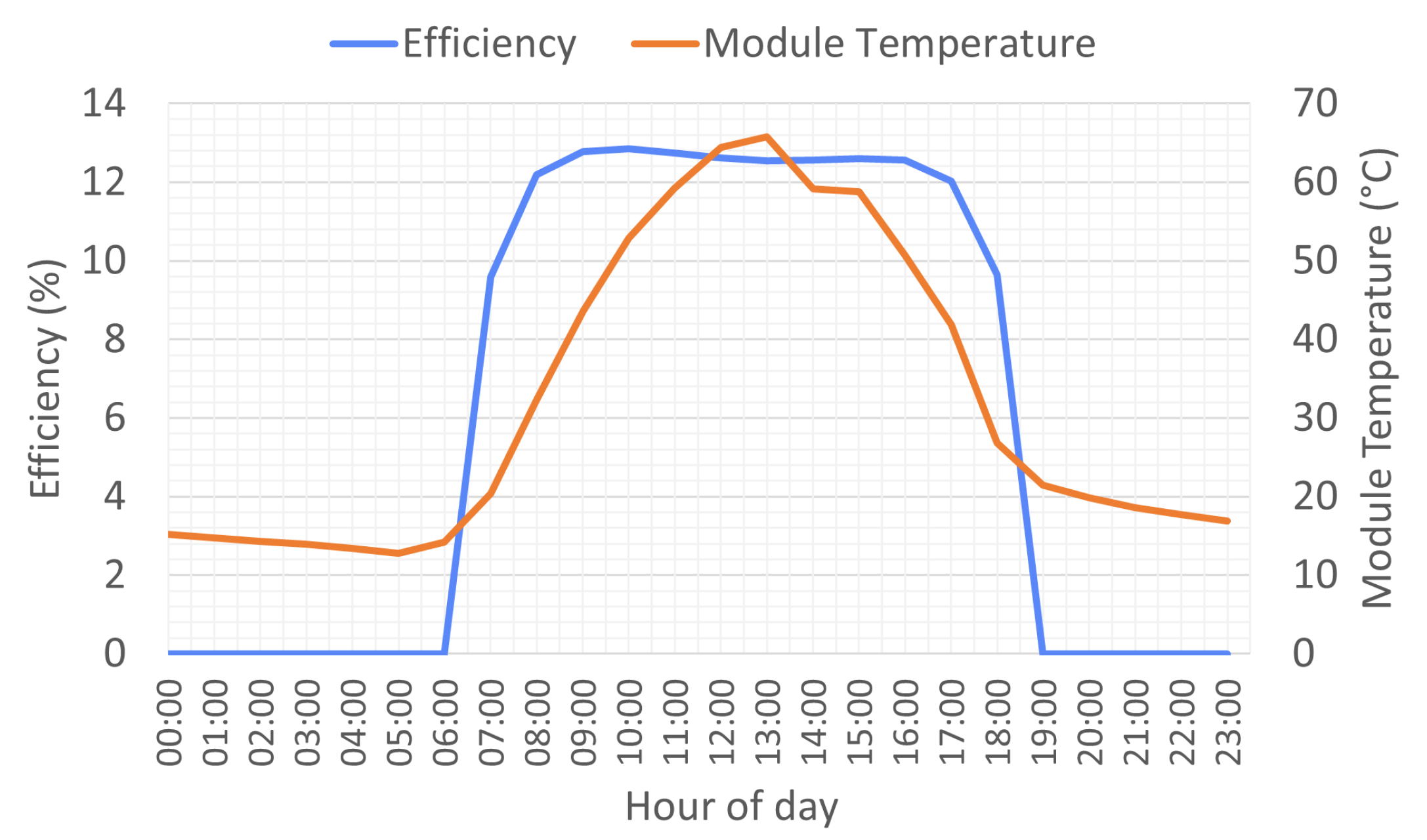
The traditional NMOT model is used in Figure 5 to display the hourly efficiency of PV panels under nonstandard conditions of irradiance and temperature considered in (24). As mentioned in Section 4, a temperature increase above the NMOT level flattens the efficiency curve, thereby negatively affecting the performance of PV modules.
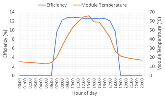
Figure 5.
Module efficiency vs. temperature.
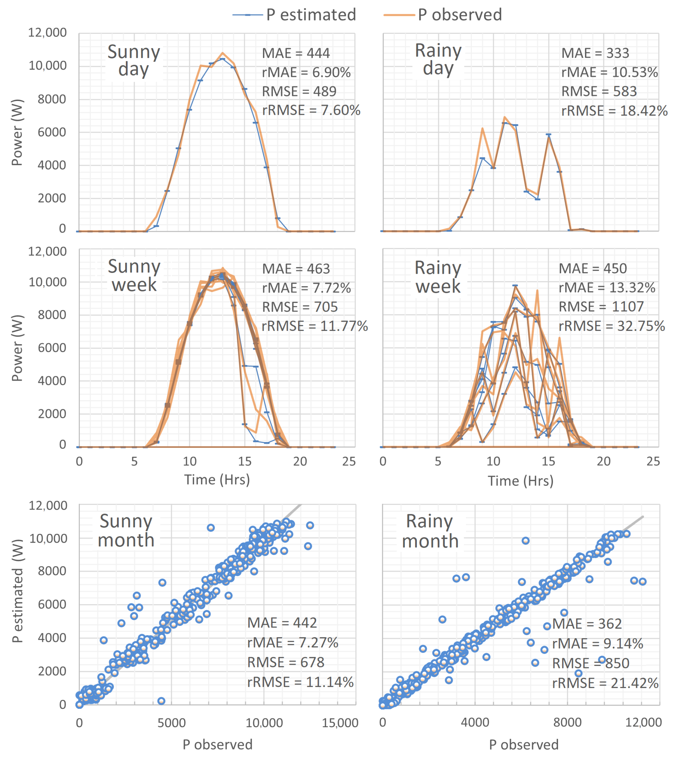
The NMOT model is used once again in Figure 6 to compare the PV power estimation performance under clear and cloudy sky conditions (i.e., sunny and rainy days). Here, lower irradiance levels on a rainy day produce lower PV power output, which leads to smaller values of MAE (i.e., MAE = 333 W). However, wider differences between observed and estimated values cause higher RMSE (i.e., RMSE = 583 W). Similarly, the variable conditions during a rainy week in September, contrasted with the stable weather conditions of a sunny week in March, clearly reflect a wider dispersion between observed and estimated values, and hence a significant increase in rMAE (from rMAE = 7.72% to 13.32%) and rRMSE (from rRMSE = 11.77% to 32.75%).
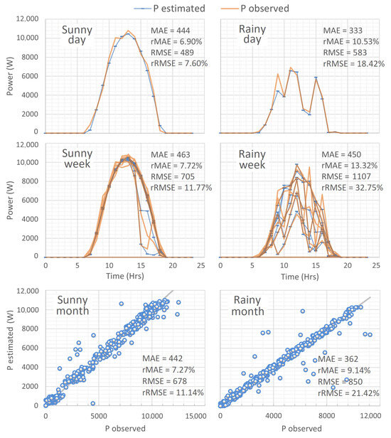
Figure 6.
Daily, weekly and monthly validation outcomes under sunny and rainy weather conditions.
In general, as the averaging period of day-ahead predictions is extended (e.g., from weekly to monthly or monthly to annual), errors tend to decrease due to the fundamental properties of averages. This is the reason why corresponding weekly error metrics can be significantly greater than monthly values in the lower part of Figure 6. Furthermore, greater dispersion is clearly identified by graphical inspection between the cloudy and rainy monthly analysis than the same case of sunny and clearly conditions.
8.1. Daily Validation
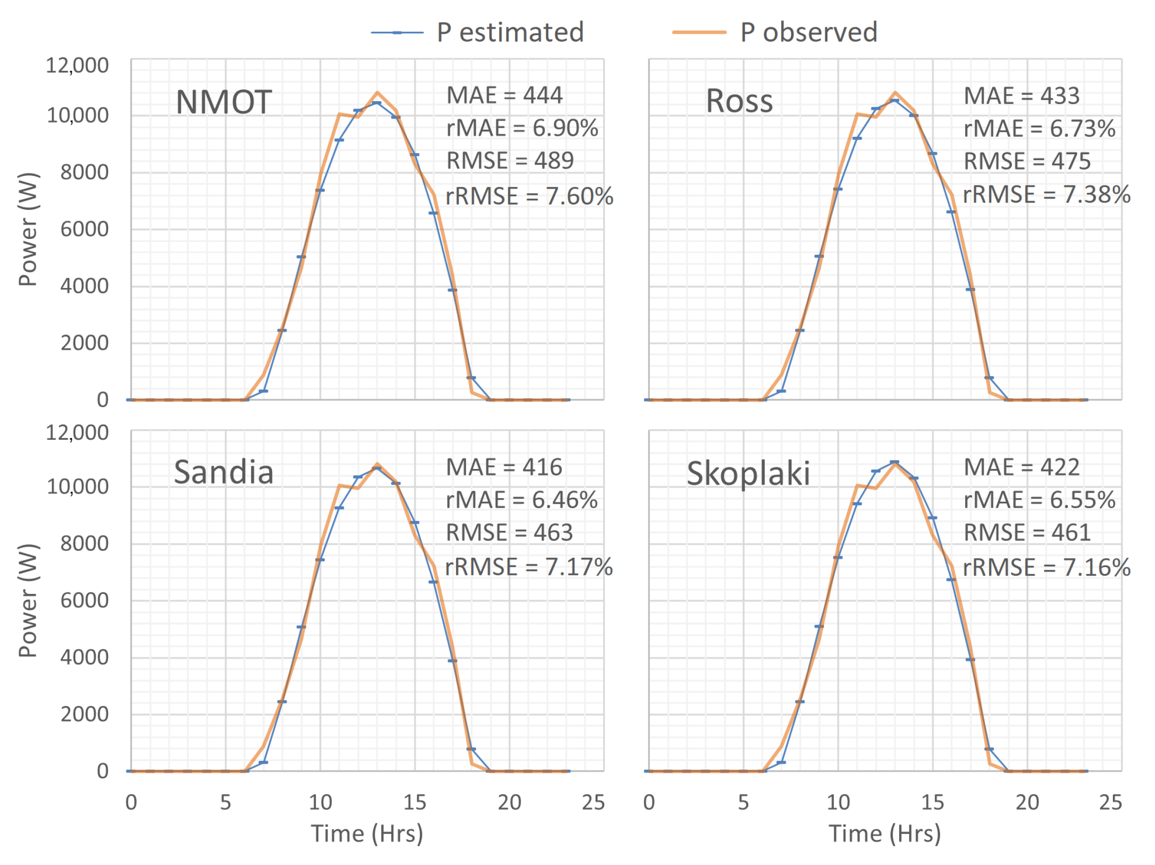
Estimated and observed values of the hourly PV power output, corresponding to a random day in March, are shown in Figure 7. Here, the PV power output estimation values are obtained by using (25) and the thermal models proposed in Section 4. As shown, low error metrics around rMAE between 6.46% and 6.9% and rRMSE between 7.16% and 7.60% reflect the high accuracy of the estimated values from the NMOT, Rosss, Sandia, and Skoplaki models. Furthermore, similar graphs and small differences among the proposed thermal models for the daily analysis are observed, with the Sandia model achieving the lowest rMAE under the corresponding weather conditions.
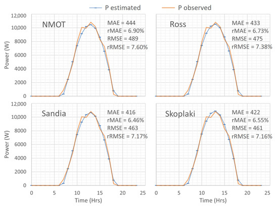
Figure 7.
Daily validation of PV power output in the case study.
8.2. Weekly Validation
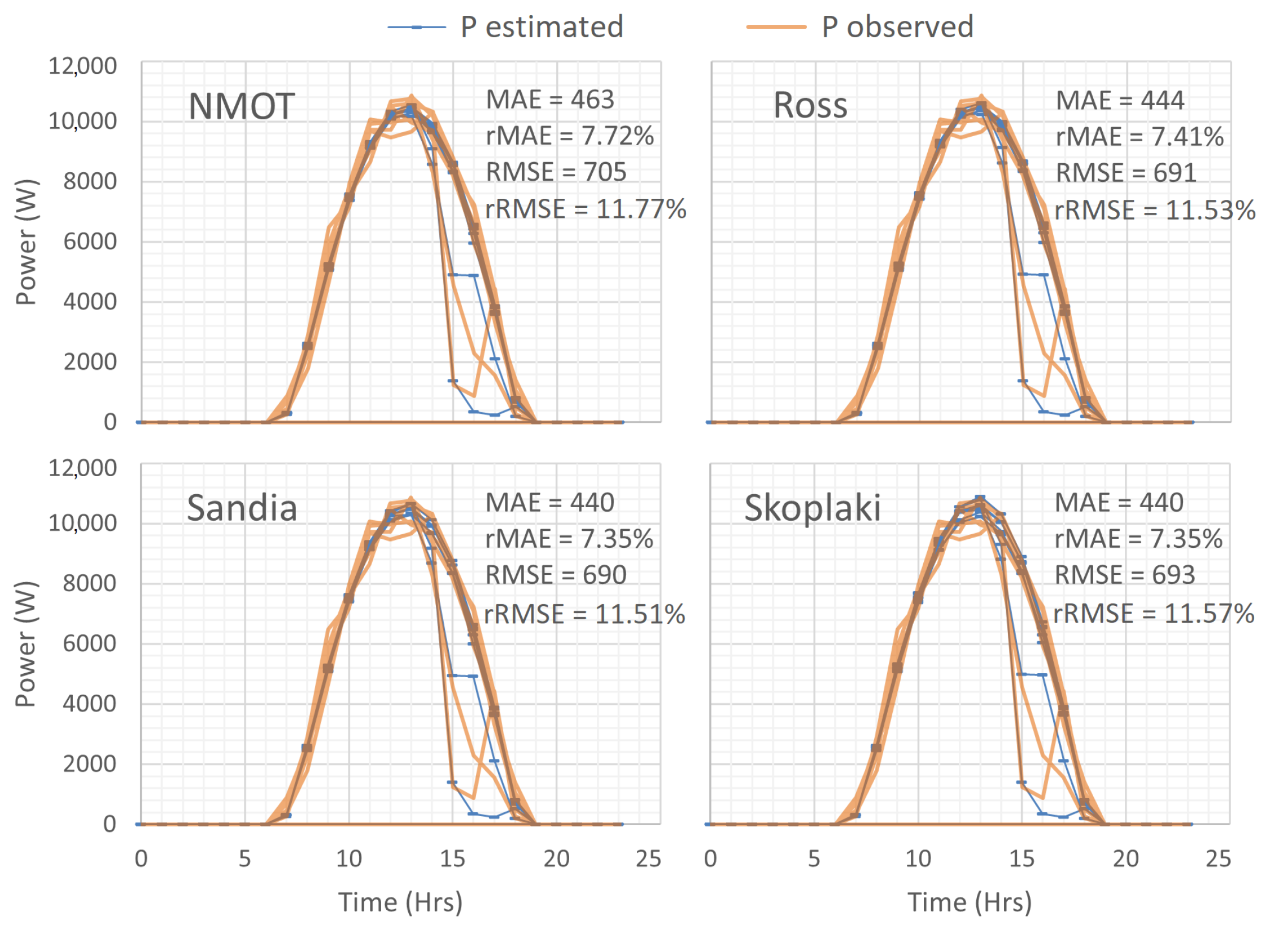
In the weekly comparison of PV power output estimation using the proposed thermal models, the averaging time for error metrics is longer than in the daily analysis. Larger differences between estimated and observed values, driven by broader weather variations, are considered. Consequently, a significant increase in the weekly error metrics is observed in Figure 8. However, smaller differences among the error metrics of the proposed thermal models are obtained. In this case, the minimum rMAE of 7.35% is achieved by the Sandia and Skoplaki models, followed closely by the Ross model with 7.41% and the NMOT model with 7.72%.
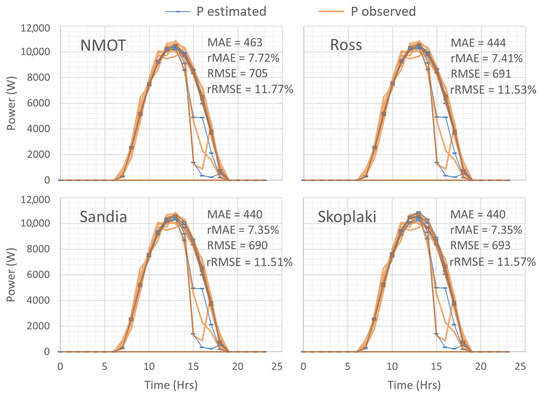
Figure 8.
Weekly validation of PV power output in the case study.
8.3. Monthly Validation
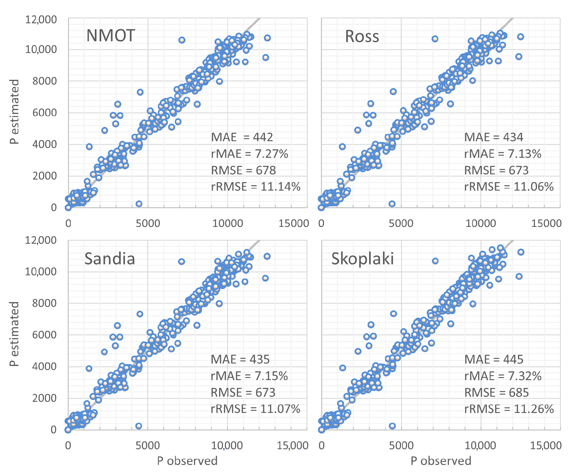
The monthly analysis in Figure 9 depicts the similarity in validation outcomes for all the proposed thermal models, performing under the same weather conditions. The Ross model achieves the lowest rMAE value (7.13%) and rRMSE value (11.06%), followed closely by the Sandia model (7.15% and 11.07%, respectively), the NMOT model (7.27% and 11.14%), and the Skoplaki model (7.32% and 11.26%).
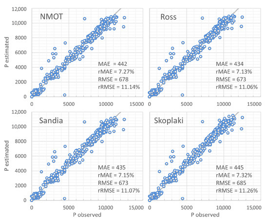
Figure 9.
Monthly validation of PV power output in the case study.
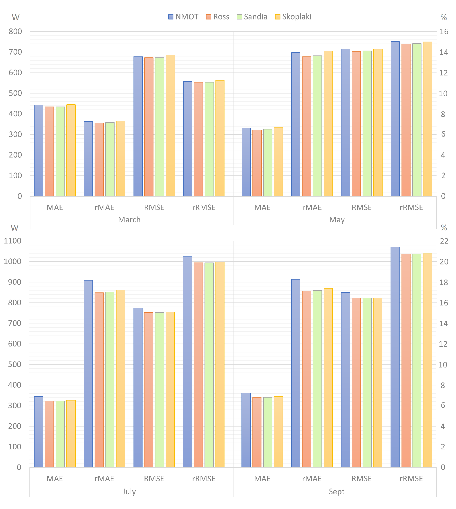
The accuracy metrics of PV power estimators in the literature report rMAE values in the range of 7.86% to 30% for the short-term horizon [18]. The monthly validation of the proposed methodology exhibits a remarkable performance, with rMAE values ranging from 6.77% to 9.14%. Figure 10 shows the accuracy metrics of all proposed models for the months of March, May, July, and September 2024. This Figure presents a column chart that clearly illustrates the performance of each thermal model evaluated in the case study. The results for the individual models exhibit strong consistency across all months, indicating stable behavior under varying conditions. Notably, the differences among the models are minimal, with rMAE and rRMSE values differing by no more than 1.2%, which underscores the overall similarity in their predictive capabilities. As shown in the Figure 10, the Ross model is the most accurate, consistently registering the lowest error values across all metrics. It is followed by the Sandia model, while the NMOT and Skoplaki models alternate in the lower accuracy positions.
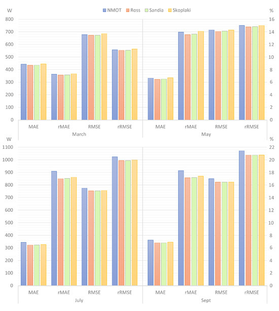
Figure 10.
PV power output validation for all proposed thermal models.
9. Conclusions
Several methods have been developed in the literature to determine, in advance, the power output capacity of PV plants. Each of these methods exhibits particular strengths, weaknesses, and areas of opportunity, depending on the application field and available resources. In this paper, some areas for improvement are identified, and a proper procedure is proposed to estimate PV power output for the short-term horizon. The effectiveness of the proposed PV power estimation algorithm relies on both the accuracy of the commercial WPD used and the performance of the utilized PV panel model. The highly correlated and similar responses of the proposed PV thermal models suggest that the Ross, Sandia, and Skoplaki models all represent viable and competitive alternative approaches to address the NMOT removal stated in the IEC 61215-1:2021 standard, with the Ross model standing out as the most accurate in this case study.
The PV power estimation algorithm developed in this paper represents an accurate tool that enables planning operators to enhance energy management strategies by calculating, in advance, the power capacity of a PV plant. Although a quantitative analysis of financial savings or emission reductions is not performed, an improved forecasting methodology enhances the reliability and sustainability of PV generation, reducing the reliance on higher-cost energy from non-renewable sources that use fossil fuels. These practices promote the integration of renewable resources into the grid and provide economic and ecological benefits for end-users and the environment.
10. Future Work
Future research will focus on extending the proposed estimation approach to other photovoltaic technologies, such as cadmium telluride (CdTe), copper indium gallium selenide (CIGS), and multijunction solar cells. These technologies present different thermal behaviors and efficiency profiles, which may affect the accuracy of power output predictions under variable environmental conditions. In addition, the methodology will be adapted to assess photovoltaic systems equipped with mobile mounting structures, such as single-axis solar trackers, where dynamic tilt angles and irradiance profiles introduce further variability in power output. These extensions will help evaluate the robustness and versatility of the proposed thermal modeling approach in broader application scenarios.
Author Contributions
Conceptualization, J.G.M.-P., M.M.-M., J.C.O.-G. and A.L.N.-G.; Methodology, J.G.M.-P., M.M.-M. and J.C.O.-G.; Software, J.G.M.-P., M.M.-M. and A.L.N.-G.; Validation, J.G.M.-P., M.M.-M. and J.C.O.-G.; Formal analysis, J.G.M.-P., M.M.-M., J.C.O.-G. and A.L.N.-G.; Investigation, J.G.M.-P., M.M.-M., J.C.O.-G. and A.L.N.-G.; Resources, J.G.M.-P., M.M.-M., J.C.O.-G. and A.L.N.-G.; Data curation, J.G.M.-P., M.M.-M., J.C.O.-G. and A.L.N.-G.; Writing—original draft, J.G.M.-P., M.M.-M., J.C.O.-G. and A.L.N.-G.; Writing—review and editing, J.G.M.-P., M.M.-M., J.C.O.-G. and A.L.N.-G.; Visualization, J.G.M.-P., M.M.-M., J.C.O.-G. and A.L.N.-G.; Supervision, J.G.M.-P., M.M.-M., J.C.O.-G. and A.L.N.-G.; Project administration, J.G.M.-P., M.M.-M., J.C.O.-G. and A.L.N.-G. All authors have read and agreed to the published version of the manuscript.
Funding
This research received no external funding.
Institutional Review Board Statement
Not applicable.
Informed Consent Statement
Not applicable.
Data Availability Statement
Data are contained within the article.
Conflicts of Interest
The authors declare no conflicts of interest.
Abbreviations
| EMS | Energy Management Systems. | |
| GW | Giga-Watt. | |
| VRE | Variable Renewable Energy. | |
| PV | Photovoltaic. | |
| NWP | Numerical Weather Prediction. | |
| WPD | Weather Prediction Data. | |
| STC | Standard Test Conditions. | |
| NTE | Nominal Terrestrial Environment. | |
| NMOT | Nominal Module Operating Temperature. | |
| INMOT | Installed Nominal Module Operating Temperature. | |
| GHI | Global Horizontal Irradiance. | |
| DHI | Diffuse Horizontal Irradiance. | |
| DNI | Direct Normal Irradiance. | |
| BHI | Beam Horizontal Irradiance. | |
| m-Si | Mono-crystalline silicon. | |
| p-Si | Poly-crystalline silicon. | |
| a-Si | Amorphous- silicon. | |
| MAE | Mean Absolute Error. | |
| rMAE | relative Mean Absolute Error. | |
| RMSE | Root Mean Square Error. | |
| rRMSE | relative Root Mean Square Error. | |
| e.g., | Exempli gratia. | |
| i.e., | Id est. | |
| P | Power capacity | W. |
| I | Irradiance | W/m2. |
| T | Temperature | °C. |
| Temperature coefficient | °C−1. | |
| Efficiency. | % | |
| Transmittance | dimensionless. | |
| a | Absorptance | dimensionless. |
| U | Thermal coefficient | W/m2°C. |
| Wind speed | m/s. | |
| m | Temperature mounting term | °C. |
| k | The Ross coefficient | °C m2/W. |
| Wind convection coefficient | m/s. | |
| Free local wind speed | m/s. | |
| The Scoplaki mounting coefficient | dimensionless. | |
| Open circuit voltage | V. | |
| Short circuit current | A. | |
| Fill factor | dimensionless. | |
| Irradiance correction factor | dimensionless. | |
| Angle of incidence | degrees. | |
| Solar zenith angle | degrees. | |
| Local latitude | degrees. | |
| Declination angle | degrees. | |
| h | Hour angle | degrees. |
| Panel tilt angle | degrees. | |
| Azimuth angle | degrees. | |
| Albedo | dimensionless. | |
| A | Aperture area | m2. |
Appendix A. Validation Metrics
Four common error metrics used in the solar energy field to assess the accuracy of forecasting models, are considered in current analysis: The Mean Absolute Error (MAE) in (A1), performs as a natural measurement of average error given its low sample variance, the Root Mean Square Error (RMSE) in (A2), considered also as a measurement of dispersion error but substantially more influenced by outliers, the relative MAE (rMAE) in (A3), provides the best practical measure of relative dispersion error, and the relative RMSE (rRMSE) in (A4) [18,50].
where and are the estimated and observed PV power, respectively, and N is the number of observations. In PV power output analysis, the MAE and RMSE are expressed in Watts (W), while the rMAE and rRMSE are typically expressed as a percentage (%).
References
- Renewables 2024: Global Status Report—REN21 Secretariat. Available online: https://www.ren21.net/reports/global-status-report/ (accessed on 15 January 2025).
- Net Zero by 2050—A Roadmap for the Global Energy Sector—International Energy Agency. Available online: https://www.iea.org/reports/net-zero-by-2050 (accessed on 15 January 2025).
- Woyte, A.; Van Thong, V.; Belmans, R.; Nijs, J. Voltage fluctuations on distribution level introduced by photovoltaic systems. IEEE Trans. Energy Convers. 2006, 21, 202–209. [Google Scholar] [CrossRef]
- IEC 61215-2:2016; Terrestrial Photovoltaic (PV) Modules—Design, Qualification and Type Approval—Part 2: Test Procedures. International Electrotechnical Commission: Geneva, Switzerland, 2016.
- IEC 61215-1:2021; Terrestrial Photovoltaic (PV) Modules—Design, Qualification and Type Approval—Part 1: Test requirements. International Electrotechnical Commission: Geneva, Switzerland, 2021.
- Trends in Photovoltaic Applications 2024: Report IEA PVPS T1-43:2024—Photovoltaic Power Systems Technology Collaboration Programme—International Energy Agency. Available online: https://iea-pvps.org/wp-content/uploads/2024/10/IEA-PVPS-Task-1-Trends-Report-2024.pdf (accessed on 3 March 2025).
- Zieher, M.; Lange, M.; Focken, U. Variable Renewable Energy Forecasting—Integration into Electricity Grids and Markets—A Best Practice Guide; vRE Discussion Series; Federal Ministry for Economic Cooperation and Development: Eschborn, Germany, 2015; p. 29. Available online: https://www.ctc-n.org/resources/variable-renewable-energy-forecasting-integration-electricity-grids-and-markets-best-0 (accessed on 15 January 2025).
- Tian, T.; Chernyakhovskiy, I. Forecasting Wind and Solar Generation: Improving System Operations, Greening the Grid; National Renewable Energy Laboratory: Golden, CO, USA, 2016; p. 2. Available online: https://www.nrel.gov/docs/fy16osti/65728.pdf (accessed on 15 January 2025).
- Tuohy, A.; Zack, J.; Haupt, S.E.; Sharp, J.; Ahlstrom, M.; Dise, S.; Grimit, E.; Mohrlen, C.; Lange, M.; Casado, M.G.; et al. Solar forecasting: Methods, challenges, and performance. IEEE Power Energy Mag. 2015, 13, 50–59. [Google Scholar] [CrossRef]
- Gupta, P.; Singh, R. Pv power forecasting based on data-driven models: A review. Int. J. Sustain. Eng. 2021, 14, 1733–1755. [Google Scholar] [CrossRef]
- Solar Forecasting Services for the Diverse Needs of the Solar Power Industry—Solar Anywhere Forecast. Available online: https://www.solaranywhere.com/products/solaranywhere-forecast/ (accessed on 15 January 2025).
- Solar Data Services, in the Cloud. Solcast: A DVN Company. Available online: https://solcast.com/ (accessed on 15 January 2025).
- Ahmed, R.; Sreeram, V.; Mishra, Y.; Arif, M.D. A review and evaluation of the state-of-the-art in PV solar power forecasting: Techniques and optimization. Renew. Sustain. Energy Rev. 2020, 124, 109792. [Google Scholar] [CrossRef]
- Dimd, B.D.; Völler, S.; Cali, U.; Midtgard, O.M. A Review of Machine Learning-Based Photovoltaic Output Power Forecasting: Nordic Context. IEEE Access 2022, 10, 26404–26425. [Google Scholar] [CrossRef]
- Iheanetu, K.J. Solar photovoltaic power forecasting: A review. Sustainability 2022, 14, 17005. [Google Scholar] [CrossRef]
- Wu, Y.-K.; Huang, C.-L.; Phan, Q.-T.; Li, Y.-Y. Completed Review of Various Solar Power Forecasting Techniques Considering Different Viewpoints. Energies 2022, 15, 3320. [Google Scholar] [CrossRef]
- Di Leo, P.; Ciocia, A.; Malgaroli, G.; Spertino, F. Advancements and Challenges in Photovoltaic Power Forecasting: A Comprehensive Review. Energies 2025, 18, 2108. [Google Scholar] [CrossRef]
- Ramirez-Vergara, J.; Bosman, L.B.; Leon-Salas, W.D.; Wollega, E. Ambient temperature and solar irradiance forecasting prediction horizon sensitivity analysis. Mach. Learn. Appl. 2021, 6, 100128. [Google Scholar] [CrossRef]
- Tayab, U.; Yang, F.; El-Hendawi, M.; Lu, J. Energy management system for a grid-connected microgrid with photovoltaic and battery energy storage system. In Proceedings of the IEEE Australian & New Zealand Control Conference (ANZCC), Melbourne, VIC, Australia, 7–8 December 2018; pp. 141–144. [Google Scholar]
- Mayer, M.J. Benefits of physical and machine learning hybridization for photovoltaic power forecasting. Renew. Sustain. Energy Rev. 2022, 168, 112772. [Google Scholar] [CrossRef]
- Khan, M.S.; Ramli, M.A.M.; Sindi, H.F.; Hidayat, T.; Bouchekara, H.R.E.H. Estimation of solar radiation on a PV panel surface with an optimal tilt angle using electric charged particles optimization. Electronics 2022, 11, 2056. [Google Scholar] [CrossRef]
- Oladigbolu, J.O.; Ramli, M.A.M.; Al-Turki, Y.A. Feasibility study and comparative analysis of hybrid renewable power system for off-grid rural electrification in a typical remote village located in Nigeria. IEEE Access 2020, 8, 171643–171663. [Google Scholar] [CrossRef]
- Mas’ud, A. Comparison of three machine learning models for the prediction of hourly PV output power in Saudi Arabia. Ain Shams Eng. J. 2022, 13, 101648. [Google Scholar] [CrossRef]
- Shivam, K.; Tzou, J.; Wu, S. A multi-objective predictive energy management strategy for residential grid-connected pv-battery hybrid systems based on machine learning technique. Energy Convers. Manag. 2021, 237, 114103. [Google Scholar] [CrossRef]
- Sun, V.; Asanakham, A.; Deethayat, T.; Kiatsiriroat, I. A new method for evaluating nominal operating cell temperature (NOCT) of unglazed photovoltaic thermal module. Energy Rep. 2020, 6, 1029. [Google Scholar] [CrossRef]
- Guidara, I.; Souissi, A.; Chaabene, M. Novel configuration and optimum energy flow management of a grid-connected photovoltaic battery installation. Comput. Electr. Eng. 2020, 85, 106677. [Google Scholar] [CrossRef]
- Randall, J.F.; Jacot, J. Is am1.5 applicable in practice? Modelling eight photovoltaic materials with respect to light intensity and two spectra. Renew. Energy 2003, 28, 1851–1864. [Google Scholar] [CrossRef]
- Anderson, A.J. Photovoltaic Translation Equations: A New Approach—Final Subcontract Report—National Renewable Energy Laboratory. 1996. Available online: https://www.osti.gov/biblio/177401 (accessed on 15 January 2025).
- REC Solar Panels: N-Peak Technology—REC Group. Available online: https://www.recgroup.com/sites/default/files/documents/information_sheet_rec_n-peak_2_series_us_rev_a.pdf (accessed on 15 January 2025).
- Mattei, M.; Notton, G.; Cristofari, C.; Muselli, M.; Poggi, P. Calculation of the polycrystalline PV module temperature using a simple method of energy balance. Renew. Energy 2006, 31, 553–567. [Google Scholar] [CrossRef]
- Trinuruk, P.; Sorapipatana, C.; Chenvidhya, D. Estimating operating cell temperature of BIPV modules in Thailand. Renew. Energy 2009, 34, 2515–2523. [Google Scholar] [CrossRef]
- Qcells Solar Panels: Q.PEAK DUO XL-G11S.3/BFG. Available online: https://us.qcells.com/q-peak-duo-xl-g11s-bfg/ (accessed on 5 May 2025).
- Huang, Y.; Huang, C.; Chen, S.; Yang, S. Optimization of module parameters for PV power estimation using a hybrid algorithm. IEEE Trans. Sustain. Energy 2020, 11, 2210–2219. [Google Scholar] [CrossRef]
- Shi, S.; Zhang, Y.; Fang, C.; Wang, Y.; Ni, A.; Fu, Z. Energy management mode of the photovoltaic power station with energy storage based on the photovoltaic power prediction. In Proceedings of the 6th International Conference on Systems and Informatics (ICSAI), Shanghai, China, 2–4 November 2019; pp. 319–324. [Google Scholar] [CrossRef]
- Santos, L.D.O.; Carvalho, P.C.M.; Filho, C.D.O. Photovoltaic cell operating temperature models: A review of correlations and parameters. IEEE J. Photovoltaics 2022, 12, 179–190. [Google Scholar] [CrossRef]
- King, D.L.; Boyson, W.E.; Kratochvil, J.A. Photovoltaic Array Performance Model—Sandia Report; Photovoltaic System Research Division—Sandia National Laboratories: Oak Ridge, TN, USA, 2004. [Google Scholar] [CrossRef]
- Skoplaki, E.; Boudouvis, A.G.; Palyvos, J.A. A simple correlation for the operating temperature of photovoltaic modules of arbitrary mounting. Sol. Energy Mater. Sol. Cells 2008, 92, 1393–1402. [Google Scholar] [CrossRef]
- Fuentes, M.K. A Simplified Thermal Model for Flat-Plate Photovoltaic Arrays. Photovoltaic System Research Division—Sandia National Laboratories. 1987. Available online: https://www.osti.gov/biblio/6802914 (accessed on 15 January 2025).
- Faiman, D. Assessing the outdoor operating temperature of photovoltaic modules. Prog. Photovoltaics Res. Appl. 2008, 16, 307–315. [Google Scholar] [CrossRef]
- IEC 61215-2:2021; Terrestrial Photovoltaic (PV) Modules—Design, Qualification and Type Approval—Part 2: Test Procedures. International Electrotechnical Commission: Geneva, Switzerland, 2021.
- Ross, R.G. Interface design considerations for terrestrial solar cell modules. In Proceedings of the 12th IEEE Photovoltaic Specialists Conference, Pasadena, CA, USA, 1 January 1976. [Google Scholar]
- Ye, Z.; Nobre, A.; Reindl, T.; Luther, J.; Reise, C. On PV module temperatures in tropical regions. Sol. Energy 2013, 88, 80–87. [Google Scholar] [CrossRef]
- Aoun, N. Outdoor testing of free standing PV module temperature under desert climate: A comparative study. Int. J. Ambient. Energy 2019, 42, 1484–1491. [Google Scholar] [CrossRef]
- Loveday, D.L.; Taki, A.H. Convective heat transfer coefficients at a plane surface on a full-scale building facade. Int. J. Heat Mass Transf. 1996, 39, 1729–1742. [Google Scholar] [CrossRef]
- Singh, P.; Ravindra, N.M. Temperature dependence of solar cell performance—An analysis. Sol. Energy Mater. Sol. Cells 2012, 101, 36–45. [Google Scholar] [CrossRef]
- Ouiqary, A.; Kheddioui, E.; Smiej, M. Evaluation of the Global Horizontal Irradiation (GHI) on the ground from the images of the second generation European meteorological satellites MSG. J. Comput. Commun. 2023, 11, 1–11. [Google Scholar] [CrossRef]
- Liu, B.; Jordan, R. Daily insolation on surfaces tilted towards equator. ASHRAE J. 1961, 10. [Google Scholar]
- Duffie, J.A.; Beckman, W.A.; Blair, N. Solar radiation. In Solar Engineering of Thermal Processes—Photovoltaics and Wind, 5th ed.; John Wiley and Sons, Inc.: Hoboken, NJ, USA, 2020; pp. 3–44. [Google Scholar]
- Lorenz, E.; Scheidsteger, T.; Hurka, J.; Heinemann, D.; Kurz, C. Regional PV power prediction for improved grid integration. Prog. Photovoltaics Res. Appl. 2011, 19, 757–771. [Google Scholar] [CrossRef]
- Hoff, T.E.; Perez, R.; Kleissl, J.; Renné, D.; Stein, J. Reporting of irradiance modeling relative prediction errors. Prog. Photovoltaics Res. Appl. 2013, 21, 1514–1519. [Google Scholar] [CrossRef]
Disclaimer/Publisher’s Note: The statements, opinions and data contained in all publications are solely those of the individual author(s) and contributor(s) and not of MDPI and/or the editor(s). MDPI and/or the editor(s) disclaim responsibility for any injury to people or property resulting from any ideas, methods, instructions or products referred to in the content. |
© 2025 by the authors. Licensee MDPI, Basel, Switzerland. This article is an open access article distributed under the terms and conditions of the Creative Commons Attribution (CC BY) license (https://creativecommons.org/licenses/by/4.0/).