Abstract
Malware detection datasets often contain a huge number of features, many of which are irrelevant, noisy, and duplicated. This issue diminishes the efficacy of Machine Learning models used for malware detection. Feature Selection (FS) is an approach commonly used to reduce the number of features in a malware detection dataset to a smaller set of features to facilitate the ease of the Machine Learning process. The Arithmetic Optimization Algorithm (AOA) is a relatively new efficient optimization algorithm that can be used for FS. This work introduces a new malware detection system called the improved AOA method for FS (AOAFS) that enhances the performance of Machine Learning techniques for malware detection. The AOAFS contains three key enhancements. First, the K-means clustering method is used to improve the initial population of the AOAFS. Second, sixteen Binary Transfer Functions are applied to model the binary solution space for FS in the AOAFS. Finally, Dynamic Opposition-based Learning is utilized to improve the mutation capability of the AOAFS. Several malware datasets were used to compare the AOAFS to four popular Machine Learning algorithms and eight famous wrapper-based optimization algorithms. Statistically, the AOAFS was evaluated using the Friedman Test for ranking the tested algorithms, while the Wilcoxon Signed-Rank Test was employed for pairwise comparisons. The results indicated that the AOAFS achieves the highest classification accuracy with the smallest feature set across all datasets.
1. Introduction
The information technology era has made the cybersecurity threat a global issue today. Due to the rapid expansion of Internet usage, malware activities have been growing exponentially. In recent years, various types of attacks have been reported, including ransomware, trojans, worms, spyware, adware, botnet-driven attacks, and phishing-based social engineering attacks [1]. These malware attacks cause significant disruption to the daily activities of individuals as well as organizations. It is very challenging for the security industry to protect devices from attacks such as these that are being identified regularly with malware detection. Most antiviruses on endpoint systems detect and discard known malware using signature-based methods.
The constant evolution of malware poses serious challenges to cybersecurity efforts worldwide. Traditional malware detection relies on signature-based detection which identifies and blocks known malware signatures. However, its efficiency degrades seriously when dealing with more sophisticated techniques from adversaries, such as code obfuscation, encryption, and polymorphism for defeating signature-based detection [2]. Due to such limitations, there is a growing reliance on heuristic and behavior-based detection techniques, which attempt to focus on the actions executed by software as an alternative to identifying malicious intent.
A malware dataset commonly contains several thousand features, which are generally very broad. In such cases, some binary values indicate the presence of certain behaviors, while the rest of the features are continuous variables used to quantify heuristic decisions.
Feature Selection (FS) is a sophisticated technique for improving malware detection performance by obtaining an optimal set of features. This helps eliminate redundant and duplicate features in the dataset, enhancing and increasing the accuracy of malware detection. The Arithmetic Optimization Algorithm (AOA) is an iterative search algorithm that uses the four basic mathematical operators: addition, subtraction, multiplication, and division. It navigates toward optimal solutions in the search space [3].
This research study focuses on designing a novel optimization-based wrapper FS method to enhance the detection capabilities of malware detection systems using optimization techniques and Machine Learning (ML) techniques. It introduces an improved AOA variation for FS in malware detection systems (known as the AOAFS). The AOAFS offers three enhancements over the AOA. The initial population of candidate solutions is improved by the K-means clustering method. Additionally, sixteen Binary Transfer Functions (BTFs) are used to model the binary solution space for FS [4]. Lastly, the Dynamic Opposition-Based Learning (DOBL) method improves exploration and exploitation capabilities [5].
The AOAFS uses a fitness function that includes classifier accuracy and the number of selected features as key parameters. The AOAFS has been validated using different ML classifiers such as K-Nearest Neighbor (KNN), Support Vector Machine (SVM), Naïve Bayes (NB), Random Forest (RF), and Multi-layer Perceptron (MLP) neural networks on eight malware detection datasets (Section 4.1). The validation process proved that the MLP classifier is the most accurate classifier that can be used in the fitness function of the AOAFS.
In addition, the AOAFS was assessed by analyzing several Binary Transfer Functions (BTFs) incorporated into its framework. The performance of the AOAFS was then compared to eight optimization-based wrapper Feature Selection (FS) algorithms using eight malware detection datasets, as outlined in -Section 4.1. Subsequently, the AOAFS was evaluated alongside four ML algorithms. Finally, the convergence behavior of the AOAFS was illustrated, and the experimental results were validated using the Friedman Test (FT) and the Wilcoxon Signed-Rank Test (WT). Overall, the experiments demonstrate the effectiveness of the AOAFS across all tested metrics.
The current research study presents four critical contributions:
- It introduces the AOAFS, an optimization-based approach for FS in malware detection datasets (Section 4).
- It utilizes a K-means clustering method to enhance the initial population (Section 5.1.4).
- It uses sixteen BTFs to model the binary solution space for FS in the AOAFS (Section 5.1.3 and Section 6.3.1).
- It incorporates the DOBL method at the end of the AOAFS optimization loop to improve its searching capabilities (Section 5.1.5).
The study includes various experiments with the AOAFS:
- Testing each of the sixteen well-known benchmark test functions (S1, S2, S3, S4, Z1, Z2, Z3, Z4, U1, U2, U3, U4, V1, V2, V3, and V4) across eight malware detection datasets.
- Ablation analysis of the AOAFS.
- Comparing the performance of the AOAFS with eight optimization-based FS algorithms using the eight malware detection datasets.
- Evaluating the effectiveness of the AOAFS against five Machine Learning algorithms (SVM, KNN, DT, LR, and MLP) using malware detection datasets.
- Convergence analysis of the AOAFS and other optimization-based wrapper FS algorithms.
- Statistically validating the performance of the AOAFS using two non-parametric statistical tests: FT and WT.
The paper is structured as follows: Section 2 provides an overview of the latest developments in FS. Section 3 explores the key concepts relevant to this investigation. Section 4 describes the malware detection datasets. Section 5 introduces the AOAFS. Section 6 presents the simulation results, comparing the AOAFS with other competing algorithms. Section 7 discusses the experimental results of the paper. Finally, Section 8 concludes the paper.
2. Related Work
This section presents a comprehensive literature review on existing methods for malware detection. Specifically, Section 2.1 explores the latest optimization-based FS techniques for malware detection. Section 2.2 examines some Machine Learning (ML) and Deep Learning (DL) approaches for enhancing malware detection. Section 2.3 explores some of the recent advances of the Ant Colony Optimization (ACO) method in malware detection and other optimization topics. Finally, Section 2.4 examines some of the recent developments of the Grey Wolf Optimizer (GWO) in the optimization field with a focus on malware and intrusion detection.
2.1. Malware Detection with Optimization Algorithms
Varma et al. [6] proposed an optimized malware detection system that uses three optimization algorithms (Bat Optimization, Cuckoo Search Optimization, and Grey Wolf Optimization) as wrapper-based FS methods for detecting malwares in the CICINvesANDMal2019 dataset. Five ML classifiers (RF, KNN, SVM, DT, and NB) were compared with the three optimization methods. The Bat Algorithm with a DT classifier reduced the features from 4115 to 518 and achieved a high accuracy of 93.73%.
Mursleen et al. [7] developed a novel prediction technique for metamorphic malware detection using the SVM classifier and the Water Wave Optimization (WWO) algorithm. They used the WWO to determine the SVM hyperparameters. This research focuses on enhancing the accuracy of detecting metamorphic malware utilizing the combination of the strength of SVM and WWO on four synthetic datasets. Mursleen et al. [7] evaluated multiple classifiers (LAD Tree, NB, SVM, and ANN) against SVM_WWO. The results indicated that SVM_WWO achieves the highest accuracy of 93%.
Mohammadi et al. [8] presented an FS-based malware detection model using the Artificial Bee Colony (ABC) algorithm. The ABC algorithm was used as a time-efficient evolutionary algorithm to enhance the result of malware detection by reducing the dimensionality of the features. This indicates that the proposed method works quickly and achieves a high accuracy of 99.18% because of the selection of the most critical features and the feature dimensionality reduction procedure.
Perakovi et al. [9] created their new dataset called SOMLAP (Swarm Optimization and ML Applied to PE Malware Detection), comprising 51,409 records of malware and benign files. They enhance the malware detection system by using Swarm Optimization algorithms (Ant Colony Optimization (ACO), Cuckoo Search Optimization (CSO), and Grey Wolf Optimization (GWO)) to minimize the features, along with ML models (KNN, NC, RF, GNB, SVM, and DT) to classify the files as benign or malicious. The ACO-DT optimization–classifier hybrid approach showed very effective performance, achieving an accuracy of 99.37%.
Alzaqebah et al. [10] introduced an improved bio-inspired metaheuristic algorithm for Intrusion Detection Systems. It is optimized by utilizing a modified Grey Wolf Optimizer (GWO) to select the most relevant features while removing irrelevant ones from the UNSWNB-15 dataset. The Extreme Learning Machine (ELM) was used as a fast classification approach and the MGWO was used to tune the ELM’s parameter. It achieved the best result accuracy, F1 score, and G-mean measure of 81%, 78%, and 84%, respectively.
Albakri et al. [11] combined the Rock Hyrax Swarm Optimization method with DL in a new detection model called RHSODL-AMD for Android malware detection. The model uses API calls and significant permissions to classify it as malware or benign. The RHSO-based FS (RHSOFS) is used to select the optimal features from the Andro-AutoPsy dataset—the Adamax optimizer and the Attention Recurrent Auto-Encoder (ARAE) model were used for Android malware detection. The model achieved 99.05% accuracy.
Fiza et al. [12] developed an Improved Chimp Optimization Algorithm (ICOA) with a Deep Neural Network Framework (DNNF) for FS and Android malware detection in IoT devices. The DNNF method has three components: raw feature preprocessing, feature representation learning, and malware detection. The second phase involves using high-level discriminative features to enhance malware identification using ICOA. A DNNF based on Long Short-Term Memory enabled effective malware detection in Android applications. The proposed ICOA-DNNF method achieved high recall results of 91.74%.
Alamro et al. [13] presented an Automated Android Malware Detection algorithm using the Optimal Ensemble Learning Approach for Cybersecurity (AAMD-OELAC) to identify and classify Android malwares. This is an ensemble learning method that uses the ML model (Least Square Support Vector Machine (LS-SVM), Kernel Extreme Learning Machine (KELM), and Regularized Random Vector Functional Link Neural Network (RRVFLN)) to detect Android malware. The Hunter–Prey Optimization (HPO) algorithm is used to tune the parameters of DL models to improve results in malware detection. AAMD-OELAC achieved an accuracy of 98.93%.
Al-Andoli et al. [14] proposed an effective ensemble method called ECDLP for malware detection. In this approach, a Deep Auto-encoder (DAE) extracts meaningful features from datasets (Drebin, NTAM, TOP-PE, DikeDataset, and ML_Android). Five DL-based models and a Neural Network as a meta-model were used. The hybrid Particle Swarm Optimization and backpropagation (PSO-BP) method was utilized to optimize the DL models. A parallel computing framework was used to increase the scalability and efficacy of the ensemble method, with a 100% accuracy rate achieved on DikeDataset and ML_Android datasets.
Hybridization is a popular improvement technique for metaheuristic algorithms. It integrates the elements of different algorithms to produce a better version, known as the hybrid algorithm [15]. This technique is also applied with AOA techniques to enhance performance. Sharma et al. [16] used a linear programming-based approach to improve the classification performance of the AOA. It was integrated with the AOA and evaluated on two aggressive datasets, the Middlebury and DIKA datasets. The experiments showed consistent performance enhancement.
2.2. Machine Learning and Deep Learning Techniques for Malware Detection
This section illustrates recent and significant works on ML and DL approaches for malware detection.
Roseline et al. [17] proposed the Deep Random Forest approach that combines the strength of DL with the interpretability of Random Forest for robust malware detection and classification. The approach demonstrates how DL models can be used to analyze visual features within malware’s binary data, significantly improving the detection of novel and sophisticated malware threats. The proposed method achieved 98.6% detection rate using the Maling dataset.
Ayeni [18] developed a security system using supervised ML approaches for malware detection. The FS method was used in the proposed model to minimize the 100,000 columns and 35 rows of features to only 20 features. Then, three ML classifiers (K-NN, DT, and RF) were applied to the malware.csv dataset to classify it as malware or benign software. The result showed the best classification. This section illustrates recent and significant works on ML and DL approaches for malware detection.
Dener and Orman [19] suggested a malware detection method that uses memory data by applying nine ML and DL models, including the LR, NB, RF, DT, Gradient Boosted Tree, Linear Vector Support Machine, MLP, Deep Feed Forward Neural Network, and LSTM algorithms, in the big data environment. The binary classification as malware or benign was generated using the CIC-MalMem-2022 dataset containing 58,596 samples. LR achieved a high accuracy of 99.97%.
Mosli et al. [20] proposed an automated malware detection method using memory forensics and information retrieval. Their approach utilized three ML models (KNN, SVM, and RF) to classify software handles as either benign or malicious. The experiments demonstrated that the RF classifier achieved the highest performance, with an accuracy of 91.4%.
Sihwail et al. [21] introduced a new method for detecting and classifying malware. This approach involves extracting memory features from memory images using memory forensic techniques. The researchers used volatility in six memory features and achieved a high classification accuracy of 98.5% using SVM. They also introduced their new memory-based dataset containing malware and benign samples. Additionally, FS evaluation showed that DLL features were given higher weight than other memory features.
Chandranegara et al. [22] used the Malimg dataset to build a DL model (VGG-16, Inception-V3, and ResNet-18) for classifying malware. The proposed method used two scenarios: scenario 1, the original dataset, and scenario 2, the under-sampled dataset. The best performance was achieved in scenario 2 when using VGG-16, which gave 94.8% accuracy.
Nikam and Deshmukh [23] introduced a malware classification model that was evaluated on the Derbin dataset, which consists of 15,036 malicious and benign samples. This research shows how performance improved when using hybrid FS techniques, such as information gain, chi-square, and feature importance techniques, on the classifier (SVM, linear regression, KNN, Decision Trees, and XGBoost) to classify samples as benign and malicious. After using hybrid FS techniques, the XGBoost classifier achieved the highest accuracy, with 98.66%.
Al-Qudah et al. [24] developed an effective one-class SVM classifier model (OCSVM) for detecting malware in a memory dump and used Principal Component Analysis (PCA) to enhance the sensitivity and efficiency of the model on the MalMemAnalysis2022 balanced dataset. They utilized ML techniques to recognize malicious behavior in memory dumps. The one-class classification PCA was used for one-class classification, achieving an accuracy of 99.4%.
Jiang et al. [25] introduced a novel visual technique to classify fileless malware using few-shot learning methods. First, they created a fileless malware dataset of 3275 records, analyzed memory dumps, and employed a binary file visualization method. They also presented the MMEL (MAML, Mean_subtraction, Euclidean_normalization, Label_Smothing) learning framework to improve the classification accuracy of 85.6%, and experiments demonstrated that this approach worked better than alternatives.
Zhang et al. [26] proposed a stacking ensemble learning framework, known as MFDroid, for Android malware detection; the security static and dynamic analysis features of the DroidMOSS app and the DroidAnalytics app, together with the results of previous research, were used as input features for the MFDroid classifier. Eight architecture components were responsible for different classification stages, including data cleaning, FS, model selection, model training, model tuning, model validating, and output prediction. Through extensive testing, MFDroid achieved superior accuracy, precision, recall, and F1 scores over baseline classifiers, as well as compared to prior ML-based work targeting Android malware detection on the same dataset. Zhang et al. [26] revealed that the Fellyph Defenseless defense mechanism was the most effective, with the average detection rate of the MFDroid models achieving 99.5% on DroidAnalytics and 96.1% on DroidMOSS.
2.3. Ant Colony Optimization Method for Malware Detection and Other Optimization Tasks
Penmatsa et al. [27] presented a hybrid optimization approach that uses the Ant Colony Optimization (ACO) algorithm for FS and Rough Set Theory (RST) to confirm the selection of features in the FS process. Specifically, the ACO simulates the foraging behavior of ants to perform FS, while RST models uncertainty by establishing relationships between features in a malware dataset. This approach provided an accuracy of 97.8 on the clamp dataset. However, it was not compared to well-known algorithms using multiple malware datasets.
Sreelaja [28] proposed a binary ACO for recognizing ransomware detection based on a signature database. Specifically, the ant agents in ACO employ a binary search to match the incoming signature hash value (a file) with the signatures in the search space. If a match exists, the file is identified as ransomware and subsequently blocked. Sreelaja has conducted experiments that demonstrated that binary ACO is better than linear search and binary search at ransomware detection.
Qi et al. [29] proposed an enhanced XMACO method that employs directional crossover (X) and directional mutation (M) for optimizing the population in ACO. The directional crossover considers the fitness values of the ant population and moves the ants towards promising regions in the search space and subsequently improves the convergence rate of ACO. The directional mutation also considers the fitness of the ant and mutates the population to increase the diversity in ACO. The experimental results on CEC 2014 and CEC 2017 benchmark sets [30,31] demonstrated that the improved ACO could jump out of local optima and improve the performance of ACO.
2.4. Grey Wolf Optimizer for Malware Detection and Other Optimization Tasks
Abed-alguni and Barhoush [32] introduced the Distributed Grey Wolf Optimizer (DGWO). The DGWO improves the original GWO by dividing the search process into multiple populations of feasible solutions. This division aims to improve exploration, exploitation, and diversity in the original GWO. The DGWO attempts to avoid local optima and achieves faster convergence by managing multiple populations of feasible solutions that communicate based on the ring topology. The experimental results on the CEC 2014 benchmark set demonstrated that the DGWO outperforms the GWO and other optimization algorithms in fitness values, accuracy, and execution time, which collectively proves the effectiveness of the DGWO for complex optimization problems.
Inspired by the success of the DGWO, Abed-alguni and Alawad [33] developed a discrete variation of the DGWO for scheduling workflow tasks in cloud computing. The Discrete DGWO employs the largest-order value (LOV) method to map the continuous search space to discrete integer space. The experimental results on WorkflowSim and scientific workflows of various sizes clearly demonstrate that the Discrete DGWO outperforms different optimization-based scheduling algorithms for cloud computing. Inspired by the DGWO, Alawad and Abed-alguni [34] modeled the CS using the principles of the DGWO (island model, ring topology, and scheduling of workflow tasks) in addition to the highly disruptive polynomial mutation method. The new algorithm was called Discrete iCSPM, and it was used with great success in solving the scheduling problem for workflow tasks in cloud computing.
Garapati and Sigappi [35] suggested EGWCSO, a combination of GWO, CS, and NB classifiers, for intrusion detection. Garapati and Sigappi [35] used the optimization operators of CS (Lévy flight-based mutation, elitist selection, and abandon and replacement [36,37,38,39]) to improve the optimization process in GWO. The experimental results on the NSL-KDD dataset showed that EGWCSO provides the most accurate detection for intrusions with the fewest possible selected features from the dataset compared to the original GWO and CS. However, EGWCSO was not evaluated with enough datasets and was not compared to state-of-the-art FS methods in the field such as the improved Binary Jaya [40], the binary opposition cellular prairie dog optimization algorithm [41], the improved Binary White Shark Optimizer [42], and the improved Opposition-based Sine Cosine method [43].
3. Background
Section 3 presents the basic concepts of our proposed method, which is organized into three subsections. Section 3.1 introduces the optimization principles. Section 3.2 illustrates Feature Selection (FS) methodologies. Finally, Section 3.3 introduces the Arithmetic Optimization Algorithm (AOA).
3.1. Optimization Problem
Optimization involves selecting inputs to achieve the best possible outputs or to enhance performance beyond current capabilities [44]. Solutions to optimization problems are assessed using an “objective function”, known as a “fitness function”. This function’s output needs to be maximized or minimized to evaluate the effectiveness of various feasible solutions [45]. The fitness function enables comparisons between these solutions to identify the optimal one. Depending on the specific nature of the problem, an optimization scenario may have a single objective or multiple objectives.
The values of the components of , which is a vector of decision variables, are computed as follows [46]:
where and are the boundaries of the decision variables. is a random generation function that generates a real number in the range [0, 1]. In binary optimization tasks, = 0 and = 1, and generates either 0 or 1.
3.2. Feature Selection
Feature Selection (FS) is a data preprocessing approach in Machine Learning and data mining [47]. FS aims to reduce the number of input variables to the predictive model, achieving better accuracy than a classifier built using the set of all features. It selects essential features while removing irrelevant and noisy ones to create a more concise data representation and save time during the learning process [48].
Figure 1 illustrates the key FS techniques, which are as follows [26]:
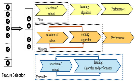
Figure 1.
The main categories of FS. Source: [26]. The symbol x represents a feature in the original dataset.
- Wrapper methods: These methods select the best subset of features from the dataset with learner intervention. They generate several subsets from the original dataset, then use the learner to evaluate each one and assess the subsets to find the best one [49].
- Filter methods: They assess features from a dataset without learners’ intervention, using statistical functions to rank each feature against all of them to indicate its importance [50].
- Embedded methods: They combine filter and wrapper methods to balance the strengths of these approaches. They apply statistical functions to rank every attribute with an intervention of the learner [48].
3.3. Arithmetic Optimization Algorithm
3.3.1. Inspiration
The main inspiration of AOA is the distribution of basic arithmetic operators in mathematics: division, multiplication, addition, and subtraction. These operators are used for optimization to select the optimum value from the candidate solutions based on certain conditions. This algorithm begins with a randomly selected candidate solution that will be evaluated by a fitness function and optimized through the optimization rules [3].
3.3.2. Mathematical Model of the AOA
The AOA starts by creating a population of feasible solutions as follows [51]:
where is an matrix that represents a population of solutions, where each row represents a feasible solution, and each column represents a variable decision. The rows are indexed from , and the columns are indexed from .
In the AOA, at the beginning of each iteration, a decision must be made on choosing one of two search phases: exploration or exploitation. The position updating in new search phases uses the Math Optimizer Accelerated (MOA) function, as defined in Equation (3) [52].
where
: the MOA value at iteration number .
: the current iteration.
: the maximum number of iterations.
: the minimum and maximum values of the accelerated function, respectively.
- -
- Exploration phase:
This phase deals with the exploratory nature of the AOA, which navigates the search space by employing two arithmetic operators, multiplication or division; due to their high dispersion, it is difficult to approach the target. To reach the near-optimal solution, the Mathematical Optimizer Accelerated (MOA) function, along with random search strategies (division or multiplication), is used in the AOA exploration phase [3].
The exploration procedure is mathematically modeled as follows [3]:
where ϵ is a tiny positive number such as 10−8 or 10−10 used to avoid division by zero or to stabilize the computation.
- -
- On the other hand, we use Equation (5) to update the Math Optimizer Probability (MOP) value [3]:where
: the Math Optimizer Probability at the ith iteration.
: the current iteration.
: the maximum number of iterations.
: the sensitivity parameter that defines the exploitation accuracy over the iterations.
- -
- Exploitation phase:
The exploitation phase of the AOA is presented here. It employs addition or subtraction arithmetic operators to update the candidate solutions. This approach is straightforward and moves toward the target because of the low dispersion of these operators. The exploitation operators improve their communications during this optimization stage to support this stage [3]. The exploitation operators of the AOA used two primary search strategies, subtraction (S) and addition (A) search strategies, to explore the search area in dense regions. The exploitation procedure is mathematically modeled as follows [53]:
where
- : the jth decision variable in .
- : the upper bound of .
- : the lower bound of .
- : a control parameter to adjust the search process.
Algorithm 1 outlines the AOA workflow, as detailed in this section.
| Algorithm 1: The AOA |
| 1: Set the initial values of and 2: Initialize the feasible solutions. 3. 4: while (< ) do 5: Calculate the fitness value for each of the feasible solutions. 6: Compute the best feasible solution. 7: Use Equation (3) to update the value of . 8: Use Equation (5) to update the value of 9: for ( to ) do 10: for ( to ) do 11: Generate three random real numbers , and in the range [0, 1] 12: if then 13: if then 14: (1) Implement division mutation (). 15: Employ the first rule in Equation (4) to mutate . 16: else 17: (2) Implement multiplication mutation (). 18: Employ the second rule in Equation (4) to mutate . 19: end if 20: else 21: if then 22: (1) Implement subtraction mutation (). 23: Mutate using the first rule in Equation (6). 24: else 25: (2) Implement addition mutation (). 26: Employ the second rule in Equation (6) to mutate . 27: end if 28: end if 29: end for 30: end for 31: 32: end while 33: Return |
4. Datasets
This section comprises two parts. Section 4.1 provides information about the malware datasets used in the experiments, and Section 4.2 provides a description of the data preprocessing steps applied to these datasets.
4.1. Data Description
In this section, we present eight popular malware detection datasets used to evaluate malware detection models’ performance. Each dataset has different labels, numbers of features, and instances. Table 1 provides the specifics for each dataset sample used to assess each algorithm employed in this research. These datasets are publicly available to use for scientific research. The data in these datasets were collected from real-world systems, so the data in the datasets reflect realistic scenarios. The datasets are pre-anonymized by the providers of the datasets, and no personally identifiable information is included in any of the eight datasets. Note that the last two columns in Table 1 specify the public availability status and the main reference for each dataset.

Table 1.
Detailed information about eight malware detection datasets. Sources: [54,55,56,57,58,59,60,61].
The datasets used are CIC-MalMem-2022, CICMalDroid-2020, CIC-AAGM2017, CICAndMal2017, TUNADROMD Dataset, EMBER-2018 Dataset, Detect Malware Types Dataset (UCI), and Drebin2-2015. These datasets are commonly used as evaluation benchmarks for malware detection systems. These high-dimensional datasets often contain imbalanced classes, missing values, unnecessary features, and diverse data types, requiring much preprocessing, like handling missing values and converting data types for classification purposes. Label encoders are crucial to maintaining unbiased classification standards [62].
4.2. Data Preprocessing
The datasets selected for this study are crucial for evaluating the performance of malware detection systems. They cover a diverse range of malware scenarios, which is essential for testing the robustness of FS methods in the AOAFS. The following preprocessing steps were applied uniformly across all datasets:
Handling missing values: Malware detection datasets frequently encounter a missing value, which can lead to biased estimates if unaddressed. This preprocessing phase uses multiple imputation strategies, leveraging predictive models to estimate missing values based on observed data. This ensures that the dataset’s integrity and distribution are maintained [63].
Balancing the datasets: Datasets usually contain class imbalances in malware detection use cases; instances of malicious software are fewer than benign. The imbalance can be biased toward the majority class; therefore, countermeasures are taken, such as the Synthetic Minority Over-sampling Technique (SMOTE) and under-sampling at random of the majority class [64]. These methods aim to achieve class distribution parity, enhancing the model’s sensitivity to the minority class. A random sample from the minority class can be computed as follows [65].
where
: a random sample from the minority class.
: one of the random neighbors of from the minority class.
λ: an interpolation factor between 0 and 1.
: the new synthetic sample.
Normalization: This step adjusts the scale of data attributes, enabling comparison on common grounds. In this paper, the Z-score normalization rescales the data with a mean () of 0 and a standard deviation (σ) of 1. This normalization is essential in our context due to the big differences between values of different features; therefore, FS algorithms will have a standard environment. It should be noted that the Boolean feature does not need any normalization. Alawad et al. [66] computed the relying on the mean () and standard deviation (σ) using Equation (8):
Encoding: Categorical variables were converted into a machine-readable format using one-hot encoding to avoid inducing ordinal relationships [62].
5. Materials and Methods
5.1. Improved Arithmetic Optimization Algorithm for Malware Detection
Figure 2 shows the flowchart of the AOAFS. It displays the phases of the AOAFS, beginning with using K-means to enhance the initial population. Then, the BTFs are utilized to model the binary solution space for FS in the AOAFS. Finally, the DOBL method is used to enhance the exploration and exploitation capabilities of the AOAFS.
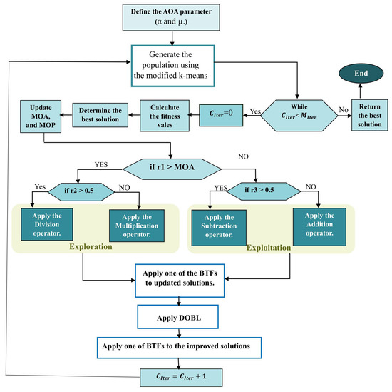
Figure 2.
The flowchart of the AOAFS. Source: Self-developed by the authors.
The details of the AOAFS are shown in Algorithm 2.
| Algorithm 2: The Improved Arithmetic Optimization Algorithm (AOAFS) |
| 1: Set the initial values of and 2: Use the enhanced K-means algorithm (Section 5.1.4) to create a population of candidate solutions from many candidate solutions (say, M). 3: 4: while (< ) do: 5: Calculate the fitness value for each of the feasible solutions using Equation (8) 6: Compute the best feasible solution. 7: Use Equation (3) to update the value of . 8: Use Equation (5) to update the value of 9: for ( to ) do 10: for ( to ) do 11: Generate three random real numbers , and in the range [0, 1]) 12: if then 13: if then 14: Implement division mutation (). 15: Mutate using the first rule in Equation (4). 16: else 17: Implement multiplication mutation (). 18: Mutate using the second rule in Equation (4). 19: end if 20: Apply one of the BTFs to updated solutions. 21: else 22: if then 23: Implement subtraction mutation (). 24: Mutate using the first rule in Equation (6). 25: else 26: Implement addition mutation (). 27: Mutate using the second rule in Equation (6). 28: end if 29: Apply one of the BTFs to updated solutions. 30: end if 31: end for 32: end for 33: Apply DOBL (Section 5.1.5) using the input parameters: , and 34: Apply one of the BTFs to the improved solutions. 35: 1 36: end while 37: Return |
Algorithm 2 sets the initial values of α and μ, then generates an initial population of feasible binary solutions using an enhanced K-means clustering algorithm (Section 5.1.4) to ensure the diversity of the population. Algorithm 2 then iteratively improves the solutions over a maximum number of iterations (). Algorithm 2 evaluates the fitness of each feasible solution at each iteration. Finally, Algorithm 2 identifies the best solution. The key control parameters, and , are updated to balance exploration and exploitation.
Specifically, the improvement loop of the AOAFS in Algorithm 2 employs mutation operations based on random selection parameters. Algorithm 2 assigns values in the range [0, 1] based on a uniform random generation function to the random selection parameters (, and ). Algorithm 2 uses these random parameters for probabilistic selection of mutation operators in the AOA and AOAFS. In each iteration of Algorithm 2, if and , then Algorithm 2 explores the population of solutions using division-based mutation. If and , then Algorithm 2 explores the population of solutions using multiplication-based mutation. If and , then Algorithm 2 goes into the exploitation phase using the subtraction-based mutation. If and , then Algorithm 2 goes into the exploitation phase using the addition-based mutation. Algorithm 2 uses the BTFs to map the mutated continuous feasible solutions to the binary domain. Afterwards, Algorithm 2 applies DOBL to explore the search areas in the opposite direction of the mutated solutions. Finally, the algorithm returns the best solution found. This procedure makes Algorithm 2 effective for solving complex optimization problems with high-dimensional search spaces such as the malware detection datasets.
5.1.1. Initialization of the AOAFS
The AOA is a population-based algorithm that begins by randomly generating a population. It then applies a sequence of rules throughout the optimization process to improve these solutions. In this work, each solution is represented as a vector of binary values (0 or 1) with a length of , where is the number of features in the original dataset, and each bit represents a single attribute. The bit value of th attribute in the ith solution denoted as , and if it equals 1, it will be selected; otherwise, it will not be selected in the subset of features [67].
Figure 3 represents a binary population of three binary feasible solutions, where each row corresponds to a candidate solution (x1, x2, x3), and each column (, , …, ) represents a feature. A value of 1 indicates that the feature is selected in that solution, while 0 means it is excluded. For example, solution x1 contains features , , …, , while x2 contains , …, . This binary representation is commonly used in optimization algorithms for Feature Selection, such as evolutionary algorithms and swarm intelligence, where each row represents a potential subset of features to evaluate in search of an optimal selection.
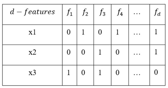
Figure 3.
Representation of three solutions for FS. Source: Self-developed by the authors.
The binary encoding procedure can be outlined as follows [68]:
5.1.2. Fitness Evaluation
All optimization problems require an objective function that evaluates the effectiveness of a solution. We aim to reduce the feature set size (i.e., the number of selected features) and enhance classification accuracy when using wrapper Feature Selection methods. In our proposed technique, we used the following objective function [62]:
where
: fitness function.
: error rate achieved by a classifier.
|R|: the upper bound of .
|N|: a control parameter to adjust the search process.
: a weight factor.
: a weight factor that is equal to 1 −
The AOA uses a Multi-Layer Perceptron (MLP) classifier as a critical component of its fitness function.
5.1.3. Binary Transfer Functions
In FS, the BTFs convert a continuous search space into a binary one. This technique is commonly used in binary classification tasks such as malware detection. BTFs transform continuous values into binary values (0 or 1), aligning with feature inclusion’s binary nature, indicating whether a feature is selected. Table 2 shows four popular families of BTFs [69,70], including S-shaped, V-shaped, Z-shaped, and U-shaped families. Four common examples are mentioned in the table for each family with their respective equations.
Table 2.
Sixteen popular BTFs. Sources: [69,70].
5.1.4. Improving Population by K-Means Clustering
The K-means method is an unsupervised ML and data analysis technique for partitioning a dataset into k clusters. Based on feature similarity, each data point is assigned to the cluster with the nearest centroid. K centroids are defined, with one for each cluster. The K-means approach improves the distribution of feasible solutions in the AOAFS by generating initial solutions from different regions in the search space.
We identified and related each point to the nearest centroid [71]. We utilized the Euclidean distance to calculate the distance between data points () and the cluster centroids (). This procedure is mathematically represented as follows [65]:
Algorithm 3 is a modified K-means algorithm [42]. It is basically a clustering-based initialization approach used to produce a diverse initial population for optimization problems. In the beginning, the algorithm randomly generates a large number (M) of candidate solutions and specifies the number of clusters (k) with random initial centroids. With each iteration of the algorithm, the algorithm assigns each of the M candidate solutions to the nearest centroid according to distance calculations using the Euclidean distance function. At the end of each iteration, the algorithm updates the centroids based on the average solution in each cluster. The algorithm only stops when the centroids stop changing. Then, one solution is randomly selected from each of the k clusters to form the initial population of k solutions.
| Algorithm 3: The modified K-means algorithm. Source: [42]. |
| 1: Generate randomly a large number (M) of candidate solutions. 2: Specify the number of k clusters and assign a random centroid to each cluster. 3: Repeat 4: Assign each candidate solution in set M to its nearest centroid based on the Euclidean distance function. 5: Compute a new centroid for each of the k clusters 6: Until the centroids are not changed 7: Select only one solution randomly from each cluster to build the initial population of k solutions with a high level of diversity. |
5.1.5. Improving Solutions Using Dynamic Opposition-Based Learning
Opposition-based Learning (OBL) provides an added advantage in space exploration. When considering a candidate solution, OBL considers its oppositional position to facilitate enhanced space exploration, helping to avoid getting stuck in local optima and guiding the search towards a more robust global solution. This approach ensures that the search is exhaustive and practical in navigating the complex landscape of high-dimensional data [72]. For a candidate solution within a bounded search space of [], the opposite is defined as follows [68]:
This is an oppositional formula: if is close to , then will be close to and vice versa [73]. DOBL uses this oppositional notion to explore both the current and its opposite points within the search space, increasing the likelihood of finding optimal or near-optimal solutions.
The DOBL method (Algorithm 4) is a novel approach of OBL that involves using OBL on a subset of decision variables () in each feasible solution to enhance optimization algorithms. Algorithm 4 considers both the candidate solution and its opposite to exploring the search space [73]. The following equation is used to calculate [40]:
where is the current iteration number and is the maximum number of iterations in the DOBL algorithm.
| Algorithm 4: The DOBL algorithm. Sources: [40,73]. |
| 1: Input: , and . 2: Calculate using Equation (14) 3: Apply OBL using Equation (9) to randomly selected design variables from 4: if is better than 5: Replace by 6: end if |
5.1.6. Evaluation of the AOAFS
The evaluation process of the AOAFS includes the following experiments:
- Comparison Between the BTFs embedded in the AOAFS.
- A cumulative comparison of the improvement embedded in our algorithm.
- Comparison between the AOAFS and eight optimization-based wrapper algorithms.
- Comparison between the AOAFS and other ML algorithms.
- Comparison between ML models embedded in the AOAFS.
- Convergence behavior of the AOAFS vs. comparative algorithms.
- Statistical analysis based on FT and WT for evaluating the significance of the experimental results.
These experiments are discussed in detail in Section 6.
6. Results
This section presents the experimental outcomes of the proposed AOAFS. The experiments are designed to investigate the AOAFS’s effectiveness in terms of classification accuracy, precision, recall, F1 score, and the size of the selected feature set, in comparison to both optimization-based wrapper algorithms and traditional Machine Learning (ML) classifiers. All results are thoroughly assessed using comparison tables, graphical representations (such as convergence plots and boxplots), and statistical analyses. The assessment in the following subsections is multi-faceted: (1) quantitative metrics (accuracy, precision, recall, F1 score, and average feature set size) are used to measure classification performance and FS efficiency, (2) convergence analysis investigates the convergence behavior in relation to iterations, while (3) non-parametric statistical tests (FT and WT) prove if the performance of the AOAFS is significantly better than the competing methods.
Specifically, the subsections include the following: “Section 6.1 Experimental Setup” details the computational environment; “Section 6.2. Evaluation Measurements” defines the performance metrics; “Section 6.3. Experimental Discussion” introduces the overall results, and “Section 6.3.1. Experiment 1: Evaluating BTFs inside the AOAFS”, “Section 6.3.2. Experiment 2: Ablation Analysis of the AOAFS”, “Section 6.3.3. Experiment 3: Evaluating the AOAFS and Optimization-based Wrapper Algorithms”, “Section 6.3.4. Experiment 4: Comparison of Performance between the AOAFS and ML Classifiers”, “Section 6.3.5. Experiment 5: Comparison Between ML Classifiers Embedded in the AOAFS”, “Section 6.3.6. Experiment 6: Convergence Analysis and Boxplots”, and “Section 6.3.7. Experiment 7: Non-parametric Statistical Analysis” provide detailed analyses, each focusing on a specific aspect of the AOAFS’s performance and its implications for malware detection, as outlined in the evaluation process described in Section 5.1.6.
6.1. Experimental Setup
We carried out our experiments on a desktop computer equipped with an Intel Core i7 processor, 16 GB of RAM, and a 512 GB SSD running Windows 11. We used Python 3.9 with libraries such as NumPy for numerical processing, Matplotlib for chart and plot illustrations, and Scikit-learn for Machine Learning.
6.2. Evaluation Measurements
To assess our experimental findings and comparisons, we employed the following assessment measures [68]: ,, , , and . measures the proportion of correctly classified instances out of the total instances. measures how many of the instances predicted as malware are actually malware. measures how many of the actual malware instances were correctly detected. is the harmonic mean of precision and recall. This measure balances the trade-off between misclassified benign files and undetected malware. is the average number of selected features across multiple runs of an FS method.
where RT is the number of iterations on each dataset, featuresii is the number of features in the best subset at each iteration, is the number of malwares accurately identified, TN is the number of benign samples accurately identified, FP is the number of benign samples recognized as malware, and FN is the number of malwares recognized as benign.
The experimental parameters are displayed in Table 3. These parameters were adopted from [35,73]. A stratified random sample technique was used to guarantee unbiased findings. Thirty percent of each dataset was dedicated for testing and seventy percent for training.
Table 3.
Parameter values. Sources: [35,73].
6.3. Experimental Discussion
This section reviews the results achieved by the proposed model across eight datasets for malware detection.
The experiments in this section assessed the performance of the AOAFS using eight datasets of malware detection records including CIC MalMem 2022 (focusing on memory-based threats), CICMalDruid 2020 and Drebin 2015 (centered on Android static analysis), CIC AAGM2017 (involving cross platform hybrids), TUNADROM D (related to ransomware), EMBER 2018 (concentrating on PE static analysis), and UCI Detect Malware Types (emphasizing anomaly detection). These datasets were chosen to cover a range of attack strategies. The results of the experiments were pretty clear about how Android datasets CICMal Droid 2020 and Drebin 2015 did not perform well compared to the rest, showing a 2 percent drop in accuracy and a 4 percent decline in precision, recall, and F1 score each. These outcomes can be attributed to the obfuscation methods such as reflection and the sparse feature representation used in these datasets. In the CIC Memory Malware Report of 2022, fileless malware showed its ability to avoid detection effectively (reaching a recall rate of 0.72), while Android ransomware known by the name TUNADROM D was found to be widespread, in 38 percent of the analyzed samples, showcasing the significance of platform diversity and the consequences of delayed software updates.
6.3.1. Experiment 1: Evaluating BTFs Inside the AOAFS
In this section, we individually tested each of the BTFs (S1, S2, S3, S4, V1, V2, V3, V4, Z1, Z2, Z3, Z4, U1, U2, U3, and U4) inside the AOAFS. Table 4 compares the BTFs using our methodology over the malware detection datasets. The best results in each table are highlighted in bold font.
Table 4.
Comparison between the BTFs incorporated in the AOAFS based on accuracy.
Specifically, Table 4 shows that using S1 is better for the CIC-MalMem-2022 dataset, S3 is better for the EMBER-2018 Dataset, S4 is better for the TUNADROMD Dataset, U1 is better for the CIC-AAGM2017 and Detect Malware Types Dataset (UCI) dataset, and Z1 is better for the CICMalDroid-2020 and CICAndMal2017 dataset. V4 is better for the Drebin2-2015 Dataset.
6.3.2. Experiment 2: Ablation Analysis of the AOAFS
In this experiment, the improvements suggested in the AOAFS are implemented in three versions: AOAFS1 (AOA and BTFs), AOAFS2 (AOA, BTFs, and K-means), and AOAFS3 (AOA, BTFs, K-means, and DOBL). Table 5 displays the accuracy of the three versions of the AOAFS. We can clearly see that the best version is AOAFS3, which incorporates all the suggested improvements into the AOA. Additionally, we can see that the performance of the AOAFS improves with the addition of each improvement method.
Table 5.
Ablation analysis of the AOAFS based on accuracy.
The bold text emphasizes the best performance values. Based on the results shown in Table 5, all the improvements we applied to the original algorithm improved the results, indicating the effectiveness of our proposed approach.
6.3.3. Experiment 3: Evaluating the AOAFS and Optimization-Based Wrapper Algorithms
This section compares the outcomes of our proposed algorithm (AOAFS) and other optimization-based wrapper algorithms (GA, PSO, ACO, SA, HS, FA, BA, and CS) performed on the datasets. Table 6 illustrates the specific parameter settings utilized in the algorithms for our methodology. These parameter values were determined based on extensive simulations on the tested algorithms.
Table 6.
The parameter setting of the tested methods. Sources: Extensive sensitive analysis of the parameters.
The evaluation was based on accuracy (Table 7), precision (Table 8), recall (Table 9), and F1 score (Table 10). As shown in Table 7, Table 8, Table 9 and Table 10, the AOAFS outperformed all other algorithms on the malware datasets. Specifically, Table 7 demonstrates that the AOAFS achieved the highest accuracy across all datasets, while Table 8 highlights its superior precision. Similarly, Table 9 indicates that the AOAFS obtained the highest recall, and Table 10 confirms that it achieved the best F1 score for all datasets.
Table 7.
The accuracy of the AOAFS vs. popular optimization-based wrapper algorithms.
Table 8.
The precision of the AOAFS vs. popular optimization-based wrapper algorithms.
Table 9.
The recall of the AOAFS vs. popular optimization-based wrapper algorithms.
Table 10.
The F1 score of the AOAFS vs. popular optimization-based wrapper algorithms.
Figure 4 shows the comparisons between nine optimization algorithms using eight malware detection datasets. The y-axis represents the number of selected features (0–60 range). Note that lower values indicate a smaller number of selected features. The AOAFS always selects the smallest number of features on all datasets, while HS, GA, and FA select the highest number of features. The number of selected features varies by dataset, which reflects dataset-specific complexity. In conclusion, the bar chart highlights the importance of choosing an algorithm that minimizes the number of selected features for a given dataset or task.
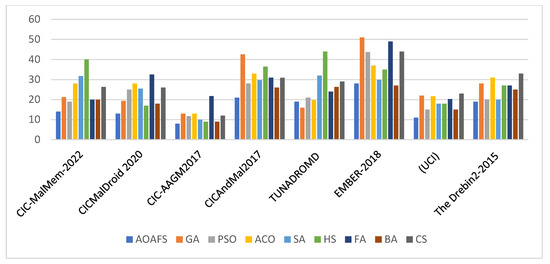
Figure 4.
The average size of feature set for the AOAFS compared with other algorithms.
Table 11 shows the feature set size across the eight malware datasets. We can see from this table that the AOAFS achieved the smallest feature set size compared to the other algorithms in seven out of the eight datasets. This offers evidence of the success of K-means clustering as an initialization method and DOBL as a mutation method in the optimization loop of the AOAFS.
Table 11.
The average feature set size for the AOAFS and the metaheuristic algorithms being compared.
6.3.4. Experiment 4: Comparison of Performance Between the AOAFS and ML Classifiers
This experiment compared our proposed AOAFS with several ML techniques, such as KNN, NB, RF, and SVM. The original KNN model used a k value of 5. We assessed the algorithms using datasets and evaluated their classification accuracy, precision, recall, and F1 score. The results in Table 12, Table 13, Table 14 and Table 15 show that our proposed method outperformed the ML models. Specifically, Table 12 demonstrates that the AOAFS achieved the highest accuracy across all datasets, while Table 13 highlights its superior precision. Table-14 shows that the AOAFS obtained the highest recall for five out of the eight datasets, and Table 15 shows that it achieved the best F1 score for seven out of the eight datasets.
Table 12.
The accuracy of the AOAFS vs. four ML models.
Table 13.
The precision of the AOAFS vs. four ML models.
Table 14.
The recall of the AOAFS vs. four ML models.
Table 15.
The F1 score of the AOAFS vs. four ML models.
6.3.5. Experiment 5: Comparison Between ML Classifiers Embedded in the AOAFS
To assess the robustness and enhancement capability of the AOAFS, its power must be judged in concert with diverse ML classifiers. This section is dedicated to evaluating the performance of the AOAFS while being coupled to SVM, KNN, DT, LR, and MLP. These classifiers are selected because they are governed by different operational paradigms, which permit an overall examination of the generalization and performance capability of the AOAFS over various ML methods. Table 16 shows the accuracy of the classifiers incorporated into the AOAFS. It is worth noting that based on Table 16, we adopted and used the MLP classifier with the AOAFS all through the experimental section of the paper.
Table 16.
The accuracy of ML classifiers is enhanced with the AOAFS.
6.3.6. Experiment 6: Convergence Analysis and Boxplots
It is necessary to analyze the AOAFS’s convergence behavior. In this section, we compare the AOAFS’s convergence rates with those of other algorithms, including Genetic Algorithm (GA), Particle Swarm Optimization (PSO), Ant Colony Optimization (ACO), Simulated Annealing (SA), and Harmony Search (HS). This comparison is based on the accuracy of each malware detection dataset. It is evaluated against other optimization-based FS methods by examining the changes in their fitness values over 50 iterations.
Figure 5 shows the convergence comparison between the AOAFS and the other five tested malware detection algorithms. In the analysis of the convergence behavior in Figure 5, we consider that an algorithm converges to an optimal solution when its accuracy value stabilizes in the range from 0.9 to 1.0.
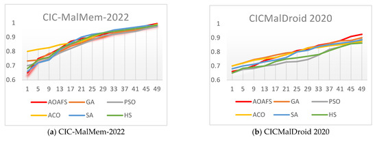
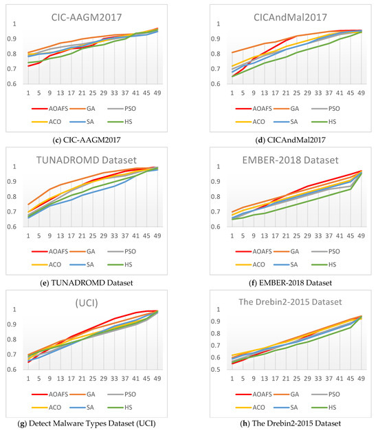
Figure 5.
Convergence behavior of the AOAFS under comparison.
Specifically, Figure 5a demonstrates that the AOAFS converges the fastest, reaching near 1.0 by around iteration 25, while ACO is the slowest, taking around 50 iterations to catch up with the rest of the algorithms. Figure 5b shows that the AOAFS again outperforms the rest of the algorithms, reaching 0.9 by iteration 15. ACO is the worst, staying below 0.8 until iteration 20. Figure 5c shows that the AOAFS and GA lead initially, with the AOAFS solely taking the lead by iteration 10. ACO is the slowest, as usual. Figure 5d illustrates that the AOAFS converges quickly, reaching around 0.9 by iteration 15. On the other hand, ACO and HS are the slowest, taking until iteration 30 to reach around 0.9. Figure 5e illustrates that the AOAFS is much faster than the other algorithms, reaching 0.9 by iteration 10. Again, ACO is the slowest, taking until iteration 35 to reach 0.9. Figure 5f shows that the AOAFS converges quickly, reaching 0.9 by iteration 15. ACO and HS are the slowest, taking until iteration 30 to reach 0.9. Figure 5g shows that the AOAFS is the fastest converging algorithm, reaching 0.9 by iteration 10, while ACO is the slowest, taking until iteration 35 to reach 0.9. Finally, Figure 5h shows that the AOAFS converges the fastest, reaching 0.9 by iteration 15. On the other hand, ACO and HS are the slowest, taking until iteration 30 to reach 0.9.
In conclusion, Figure 5 shows that the AOAFS consistently is the fastest to converge across all datasets. It often reaches 0.9 within 10–15 iterations. It also tends to achieve the highest final value, though the difference is small (around 0.01–0.02).
The boxplots in Figure 6 illustrate the Feature Selection performance across four malware datasets: CIC-MalMem-2022, CICMalDroid 2020, EMBER-2018, and Drebin2-2015. Notably, the AOAFS consistently achieves the smallest feature subset size among all compared methods, indicating superior efficiency. Furthermore, the AOAFS demonstrates lower variability and greater reliability in Feature Selection, as evidenced by its compact interquartile ranges and stable performance across diverse datasets.
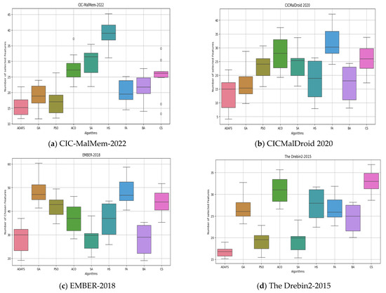
Figure 6.
Boxplots of the size of the feature set on malware datasets.
6.3.7. Experiment 7: Non-Parametric Statistical Analysis
The Friedman Test (FT) was used to measure differences among multiple related samples based on the average size of the feature set for various tested algorithms. This non-parametric test is employed when three or more associated samples are measured on an ordinal or continuous scale. Table 17, derived from Table 11, presents the size of the feature set for the AOAFS compared to other algorithms based on the FT. The AOAFS achieved the highest rank across six datasets. We utilized the WT to compare the pairwise differences between the AOAFS and other metaheuristic algorithms using the p-value to test the null hypothesis. A p-value greater than 0.05 retained the hypothesis, while a p-value less than 0.05 rejected the hypothesis [74].
Table 17.
The FT is based on the average size of the set of features for all tested algorithms.
Table 18 presents the results of pairwise comparisons of algorithms using the WT. We can clearly observe from the table that the AOAFS showed significant differences from GA, PSO, ACO, SA, HS, FA, BA, and CS. This strongly suggests that the differences between the AOAFS and the other algorithms are unlikely to have occurred by chance based on the WT.
Table 18.
WT for the average size of the set of features for all tested algorithms.
7. Discussion and Limitations
The results obtained from the experiments in Section 7 showed the average accuracy of the AOAFS for all malware datasets was around 97.9%. Specifically, the AOAFS outperformed other competitors by at least a margin of 2 to 3 percent over all the datasets. The average precision is around 97.5%, and the average recall value is about 97.9%, which proves that the AOAFS identified more true positives while minimizing false positives and false negatives, which is critical in malware detection.
The experimental results demonstrated that the AOAFS is efficient in enhancing the process of FS and malware detection. The AOAFS enhanced the efficiency of classification systems for malware detection datasets with various sizes. The AOAFS not only improves the accuracy of the classification but also makes it more focused and efficient, which significantly reduces the computational burden. The AOAFS is critical to ongoing efforts aimed at enhancing ML applications for malware detection. The AOAFS represents a promising solution to combat the constantly evolving landscape of cybersecurity threats by providing a robust and adaptable approach. Moreover, the results of the statistical WT and RT provide strong statistical evidence that our algorithm performs significantly better than the compared methods.
The AOAFS is a powerful tool for solving real-world optimization problems that can be modeled as binary optimization problems, such as the FS problem in malware detection tasks. However, it is not suitable for non-binary optimization challenges, such as the job shop scheduling problem or resource-constrained scheduling problems. In high-stakes domains like medical diagnosis, banking, and finance, critical decisions can significantly impact human lives. Hence, the interpretability of decision-making processes is critical for human lives. Therefore, Explainable Artificial Intelligence (XAI) methods such as SHAP (SHapley Additive Explanations) and LIME (Local Interpretable Model-Agnostic Explanations) can be used to justify the reasoning behind the decisions of the AOAFS. Moreover, LIME and SHAP have the capabilities to enhance the interpretability and transparency of the AOAFS or any Machine Learning model. This makes the results more accessible and understandable for humans.
8. Conclusions and Future Work
This paper introduced the AOAFS for malware detection, a significant advancement in the FS process. The AOAFS implements several improvements, including K-means, DOBL, and BTFs, to create a new technique for selecting the essential features from datasets for classification tasks such as malware detection, which focused on the performance comparison of the AOAFS with classic ML methods, focusing on its capability for optimizing FS processes.
These are achieved through a critical comparative study of the overall performance of different established datasets in cybersecurity. The research work presented in this paper implemented a rigorous statistical study and performance evaluation to determine the accuracy, precision, recall, and F1 score of the AOAFS compared with standard algorithms such as KNN, NB, RF, and SVM. Different comparative studies provided results that shed light on the performance of the AOAFS compared to the other algorithms. The AOAFS turned out to perform with consistent dominance on all considered datasets including but not limited to CIC-MalMem-2022, CICMalDroid 2020, CIC-AAGM2017, CICAndMal2017, TUNADROMD Dataset, EMBER-2018 Dataset, Detect Malware Types Dataset (UCI), and Drebin2-2015 Dataset. In all cases, the best results were contributed by the AOAFS, including improvements in precision, recall, and F1 score.
The results obtained from the experiments showed the accuracy of the AOAFS over CIC-MalMem-2022 with 99.9%. The AOAFS continued outperforming other algorithms by at least a margin of 2 to 3 percentage points concerning accuracy observed under different datasets. Also, the precision and recall measures have proved that the AOAFS identified more true positives while minimizing false positives and false negatives, which is critical in malware detection. Results demonstrated that the AOAFS’s efficiency in enhancing the process of FS is crucial to enhancing the performance of malware detection systems. High-dimensional feature extraction of only the most essential features by the AOAFS enhances the efficiency of classification systems while dealing with complex and large datasets. This helps in making the process of classification not only more accurate but also more directed with reduced computational burden.
In most datasets, the high efficiency of the AOAFS is a plus for flexibility, hence positioning it as one of the significant milestones in cybersecurity. This research is essential to continued attempts at improving ML applications for malware detection. It presents a possible method for fighting the ever-changing cybersecurity threats.
The AOAFS may serve as the foundation for several potential future research studies. First, integrating the island model (i.e., an efficient distributed optimization model) into the AOAFS to improve its execution time. Second, using the AOAFS in multi-objective FS in malware detection systems. Finally, integrating the Q-learning algorithm (i.e., one of the basic reinforcement learning algorithms) with the AOAFS to improve its exploration and convergence behaviors.
Author Contributions
Conceptualization, R.A.; methodology, R.A. and B.H.A.-a.; software, Y.E.A.; validation, Y.E.A. and B.H.A.-a.; formal analysis, R.A.; investigation, R.A. and B.H.A.-a.; resources, R.A. and B.H.A.-a.; data curation, Y.E.A. and B.H.A.-a.; writing—original draft preparation, R.A.; writing—review and editing, R.A., B.H.A.-a. and Y.E.A.; visualization, Y.E.A.; supervision, R.A.; project administration, R.A.; funding acquisition, R.A., B.H.A.-a. and Y.E.A. All authors have read and agreed to the published version of the manuscript.
Funding
This research was supported by the Scientific Research Deanship at Yarmouk University.
Institutional Review Board Statement
This article does not contain any studies with human participants or animals performed by any of the authors.
Informed Consent Statement
Not applicable.
Data Availability Statement
CIC-MalMem-2022 dataset: https://www.unb.ca/cic/datasets/malmem-2022.html (accessed on 15 March 2025); CICMalDroid-2020 dataset: https://www.unb.ca/cic/datasets/maldroid-2020.html (accessed on 15 March 2025); CIC-AAGM2017 dataset: https://www.unb.ca/cic/datasets/android-adware.html (accessed on 15 March 2025); CICAndMal2017 dataset: https://www.unb.ca/cic/datasets/andmal2017.html (accessed on 15 March 2025); TUNADROMD dataset: https://archive.ics.uci.edu/dataset/813/tunadromd (accessed on 15 March 2025); EMBER-2018 dataset: https://github.com/elastic/ember (accessed on 15 March 2025); Detect Malware Types dataset (UCI): https://archive.ics.uci.edu/ml/datasets/Detect+Malware+Types (accessed on 15 March 2025); Drebin2-2015 dataset: https://drebin.mlsec.org/ (accessed on 15 March 2025).
Conflicts of Interest
The authors declare no conflicts of interest.
Abbreviations
| AOA | Arithmetic Optimization Algorithm |
| AOAFS | Arithmetic Optimization Algorithm for Feature Selection |
| FS | Feature Selection |
| ML | Machine Learning |
| DL | Deep Learning |
| KNN | K-Nearest Neighbor |
| SVM | Support Vector Machine |
| NB | Naïve Bayes |
| RF | Random Forest |
| DT | Decision Tree |
| MLP | Multi-layer Perceptron |
| LR | Logistic Regression |
| BTFs | Binary Transfer Functions |
| DOBL | Dynamic Opposition-Based Learning |
| GA | Genetic Algorithm |
| PSO | Particle Swarm Optimization |
| ACO | Ant Colony Optimization |
| GWO | Grey Wolf Optimizer |
| SA | Simulated Annealing |
| HS | Harmony Search |
| FA | Firefly Algorithm |
| BA | Bat Algorithm |
| CS | Cuckoo Search |
| SMOTE | Synthetic Minority Over-sampling Technique |
| XGBoost | Extreme Gradient Boosting |
| OBL | Opposition-Based Learning |
| FT | Friedman Test |
| WT | Wilcoxon Signed-Rank Test |
References
- Albishry, N.; AlGhamdi, R.; Almalawi, A.; Khan, A.I.; Kshirsagar, P.R.; Debtera, B. An Attribute Extraction for Automated Malware Attack Classification and Detection Using Soft Computing Techniques. Comput. Intell. Neurosci. 2022, 2022, 5061059. [Google Scholar] [CrossRef]
- Almajed, H.; Alsaqer, A.; Frikha, M. Imbalance Datasets in Malware Detection: A Review of Current Solutions and Future Directions. Int. J. Adv. Comput. Sci. Appl. 2025, 16, 1323–1335. [Google Scholar] [CrossRef]
- Abualigah, L.; Diabat, A.; Mirjalili, S.; Elaziz, M.A.; Gandomi, A.H. The Arithmetic Optimization Algorithm. Comput. Methods Appl. Mech. Eng. 2021, 376, 113609. [Google Scholar] [CrossRef]
- Barhoush M, Abed-alguni BH, Al-qudah NE. Improved discrete salp swarm algorithm using exploration and exploitation techniques for feature selection in intrusion detection systems. The Journal of Supercomputing. 2023, 79(18), 21265–21309. [CrossRef]
- Alawad, N.A.; Abed-Alguni, B.H.; Shakhatreh, A.M. EBAO: An intrusion detection framework for wireless sensor networks using an enhanced binary Aquila Optimizer. Knowl. -Based Syst. 2025, 312, 113156. [Google Scholar] [CrossRef]
- Varma P, R.K.; Mallidi, S.K.R.; Jhansi K, S.; Latha D, P. Bat optimization algorithm for wrapper-based feature selection and performance improvement of android malware detection. IET Netw. 2021, 10, 131–140. [Google Scholar] [CrossRef]
- Mursleen, M.; Bist, A.S.; Kishore, J. A support vector machine water wave optimization algorithm based prediction model for metamorphic malware detection. Int. J. Recent Technol. Eng. 2019, 7, 1–8. [Google Scholar]
- Mohammadi, F.G.; Shenavarmasouleh, F.; Amini, M.H.; Arabnia, H.R. Malware detection using artificial bee colony algorithm. In Proceedings of the Adjunct Proceedings of the 2020 ACM International Joint Conference on Pervasive and Ubiquitous Computing and Proceedings of the 2020 ACM International Symposium on Wearable Computers, Virtual, 12–17 September 2020; pp. 568–572. [Google Scholar]
- Kattamuri, S.J.; Penmatsa, R.K.V.; Chakravarty, S.; Madabathula, V.S.P. Swarm Optimization and Machine Learning Applied to PE Malware Detection towards Cyber Threat Intelligence. Electronics 2023, 12, 342. [Google Scholar] [CrossRef]
- Alzaqebah, A.; Aljarah, I.; Al-Kadi, O.; Damaševičius, R. A Modified Grey Wolf Optimization Algorithm for an Intrusion Detection System. Mathematics 2022, 10, 999. [Google Scholar] [CrossRef]
- Albakri, A.; Alhayan, F.; Alturki, N.; Ahamed, S.; Shamsudheen, S. Metaheuristics with Deep Learning Model for Cybersecurity and Android Malware Detection and Classification. Appl. Sci. 2023, 13, 2172. [Google Scholar] [CrossRef]
- Vasu G, T.; Fiza, S.; Kumar, A.K.; Devi, V.S.; Kumar, C.N.; Kubra, A. Improved chimp optimization algorithm (ICOA) feature selection and deep neural network framework for internet of things (IOT) based android malware detection. Meas. Sens. 2023, 28, 100785. [Google Scholar] [CrossRef]
- Alamro, H.; Mtouaa, W.; Aljameel, S.; Salama, A.S.; Hamza, M.A.; Othman, A.Y. Automated Android Malware Detection Using Optimal Ensemble Learning Approach for Cybersecurity. IEEE Access 2023, 11, 72509–72517. [Google Scholar] [CrossRef]
- Al-Andoli, M.N.; Sim, K.S.; Tan, S.C.; Goh, P.Y.; Lim, C.P. An Ensemble-Based Parallel Deep Learning Classifier With PSO-BP Optimization for Malware Detection. IEEE Access 2023, 11, 76330–76346. [Google Scholar] [CrossRef]
- Gaber, M.G.; Ahmed, M.; Janicke, H. Malware detection with artificial intelligence: A systematic literature review. ACM Comput. Surv. 2024, 56, 1–33. [Google Scholar] [CrossRef]
- Sharma, S.; Krishna, C.R.; Sahay, S.K. Detection of advanced malware by machine learning techniques. In Soft Computing: Theories and Applications: Proceedings of SoCTA 2017; Springer: Berlin/Heidelberg, Germany, 2019; pp. 333–342. [Google Scholar]
- Roseline, S.A.; Geetha, S.; Kadry, S.; Nam, Y. Intelligent Vision-Based Malware Detection and Classification Using Deep Random Forest Paradigm. IEEE Access 2020, 8, 206303–206324. [Google Scholar] [CrossRef]
- Ayeni, O.A. A Supervised Machine Learning Algorithm for Detecting Malware. J. Internet Technol. Secur. Trans. 2022, 10, 764–769. [Google Scholar] [CrossRef]
- Dener, M.; Ok, G.; Orman, A. Malware detection using memory analysis data in big data environment. Appl. Sci. 2022, 12, 8604. [Google Scholar] [CrossRef]
- Mosli, R.; Li, R.; Yuan, B.; Pan, Y. A Behavior-Based Approach for Malware Detection; Springer International Publishing: Cham, Switzerland, 2017; pp. 187–201. [Google Scholar] [CrossRef]
- Sihwail, R.; Omar, K.; Ariffin, K.A.Z. An Effective Memory Analysis for Malware Detection and Classification. Comput. Mater. Contin. 2021, 67, 2301–2320. [Google Scholar] [CrossRef]
- Chandranegara, D.R.; Djawas, J.S.; Nurfaizi, F.A.; Sari, Z. Malware Image Classification Using Deep Learning InceptionResNet-V2 and VGG-16 Method. J. Online Inform. 2023, 8, 61–71. [Google Scholar] [CrossRef]
- Nikam, U.V.; Deshmukh, V.M. Hybrid Feature Selection Technique to classify Malicious Applications using Machine Learning approach. J. Integr. Sci. Technol. 2024, 12, 702. Available online: https://pubs.thesciencein.org/journal/index.php/jist/article/view/a702 (accessed on 31 October 2024).
- Al-Qudah, M.; Ashi, Z.; Alnabhan, M.; Abu Al-Haija, Q. Effective One-Class Classifier Model for Memory Dump Malware Detection. J. Sens. Actuator Netw. 2023, 12, 5. [Google Scholar] [CrossRef]
- Jiang, L.; Zhang, Y.; Shi, Y. Visual fileless malware classification via few-shot learning. In Proceedings of the International Conference on Cyber Security, Artificial Intelligence, and Digital Economy (CSAIDE 2023), Nanjing, China, 3–5 March 2023; Volume 12718, pp. 113–124. [Google Scholar]
- Zhang, Y.; Liu, R.; Wang, X.; Chen, H.; Li, C. Boosted binary Harris hawks optimizer and feature selection. Eng. Comput. 2020, 37, 3741–3770. [Google Scholar] [CrossRef]
- Penmatsa, R.K.V.; Kalidindi, A.; Mallidi, S.K.R. Feature reduction and optimization of malware detection system using ant colony optimization and rough sets. Int. J. Inf. Secur. Priv. 2020, 14, 95–114. [Google Scholar] [CrossRef]
- Sreelaja, N.K. Ant Colony Optimization based Light weight Binary Search for efficient signature matching to filter Ransomware. Appl. Soft Comput. 2021, 111, 107635. [Google Scholar] [CrossRef]
- Qi, A.; Zhao, D.; Yu, F.; Heidari, A.A.; Wu, Z.; Cai, Z.; Alenezi, F.; Mansour, R.F.; Chen, H.; Chen, M. Directional mutation and crossover boosted ant colony optimization with application to COVID-19 X-ray image segmentation. Comput. Biol. Med. 2022, 148, 105810. [Google Scholar] [CrossRef]
- Abed-Alguni, B.H.; Alawad, N.A.; Barhoush, M.; Hammad, R. Exploratory cuckoo search for solving single-objective optimization problems. Soft Comput. 2021, 25, 10167–10180. [Google Scholar] [CrossRef]
- Abed-Alguni, B.H.; Paul, D. Island-based Cuckoo Search with elite opposition-based learning and multiple mutation methods for solving optimization problems. Soft Comput. 2022, 26, 3293–3312. [Google Scholar] [CrossRef]
- Abed-Alguni, B.H.; Barhoush, M. Distributed grey wolf optimizer for numerical optimization problems. Jordanian J. Comput. Inf. Technol. (JJCIT) 2018, 4, 21. [Google Scholar]
- Abed-Alguni, B.H.; Alawad, N.A. Distributed Grey Wolf Optimizer for scheduling of workflow applications in cloud environments. Appl. Soft Comput. 2021, 102, 107113. [Google Scholar] [CrossRef]
- Alawad, N.A.; Abed-Alguni, B.H. Discrete Island-Based Cuckoo Search with Highly Disruptive Polynomial Mutation and Opposition-Based Learning Strategy for Scheduling of Workflow Applications in Cloud Environments. Arab. J. Sci. Eng. 2021, 46, 3213–3233. [Google Scholar] [CrossRef]
- Nadu, T. An enhanced Grey Wolf optimizer Cuckoo search optimization with Naïve Bayes classifier for intrusion detection system. J. Inf. Optim. Sci. 2024, 45, 2227–2236. [Google Scholar] [CrossRef]
- Abed-Alguni, B.H. Action-selection method for reinforcement learning based on cuckoo search algorithm. Arab. J. Sci. Eng. 2018, 43, 6771–6785. [Google Scholar] [CrossRef]
- Alkhateeb, F.; Abed-Alguni, B.H. A hybrid cuckoo search and simulated annealing algorithm. J. Intell. Syst. 2019, 28, 683–698. [Google Scholar] [CrossRef]
- Abed-Alguni, B.H.; Alkhateeb, F. Intelligent hybrid cuckoo search and β-hill climbing algorithm. J. King Saud Univ. Comput. Inf. Sci. 2020, 32, 159–173. [Google Scholar] [CrossRef]
- Alkhateeb, F.; Abed-Alguni, B.H.; Al-Rousan, M.H. Discrete hybrid cuckoo search and simulated annealing algorithm for solving the job shop scheduling problem. J. Supercomput. 2022, 78, 4799–4826. [Google Scholar] [CrossRef]
- Abed-Alguni, B.H.; Al-Jarah, S.H. IBJA: An improved binary DJaya algorithm for feature selection. J. Comput. Sci. 2024, 75, 102201. [Google Scholar] [CrossRef]
- Abed-Alguni, B.H.; Alzboun, B.M.; Alawad, N.A. BOC-PDO: An intrusion detection model using binary opposition cellular prairie dog optimization algorithm. Clust. Comput. 2024, 27, 14417–14449. [Google Scholar] [CrossRef]
- Alawad, N.A.; Abed-Alguni, B.H.; Al-Betar, M.A.; Jaradat, A. Binary improved white shark algorithm for intrusion detection systems. Neural Comput. Appl. 2023, 35, 19427–19451. [Google Scholar] [CrossRef]
- Abed-Alguni, B.H.; Alawad, N.A.; Al-Betar, M.A.; Paul, D. Opposition-based sine cosine optimizer utilizing refraction learning and variable neighborhood search for feature selection. Appl. Intell. 2022, 53, 13224–13260. [Google Scholar] [CrossRef]
- Abualigah, L.; Yousri, D.; Elaziz, M.A.; Ewees, A.A.; Al-Qaness, M.A.; Gandomi, A.H. Aquila Optimizer: A novel meta-heuristic optimization algorithm. Comput. Ind. Eng. 2021, 157, 107250. [Google Scholar] [CrossRef]
- Gambella, C.; Ghaddar, B.; Naoum-Sawaya, J. Optimization problems for machine learning: A survey. Eur. J. Oper. Res. 2021, 290, 807–828. [Google Scholar] [CrossRef]
- Alawad, N.A.; Abed-Alguni, B.H.; Saleh, I.I. Improved arithmetic optimization algorithm for patient admission scheduling problem. Soft Comput. 2024, 28, 5853–5879. [Google Scholar] [CrossRef]
- Li, J.; Cheng, K.; Wang, S.; Morstatter, F.; Trevino, R.P.; Tang, J.; Liu, H. Feature Selection: A Data Perspective. ACM Comput. Surv. 2017, 50, 1–45. [Google Scholar] [CrossRef]
- Theng, D.; Bhoyar, K.K. Feature selection techniques for machine learning: A survey of more than two decades of research. Knowl. Inf. Syst. 2024, 66, 1575–1637. [Google Scholar] [CrossRef]
- Spolaôr, N.; Monard, M.C.; Tsoumakas, G.; Lee, H.D. A Systematic Review of Multi-Label Feature Selection and a New Method Based on Label Construction. Neurocomputing 2016, 180, 3–15. [Google Scholar] [CrossRef]
- Emmanuel, I.; Sun, Y.; Wang, Z. A machine learning-based credit risk prediction engine system using a stacked classifier and a filter-based feature selection method. J. Big Data 2024, 11, 1–14. [Google Scholar] [CrossRef]
- Dhal, K.G.; Sasmal, B.; Das, A.; Ray, S.; Rai, R. A comprehensive survey on arithmetic optimization algorithm. Arch. Comput. Methods Eng. 2023, 30, 3379–3404. [Google Scholar] [CrossRef]
- Baş, E. Hybrid the arithmetic optimization algorithm for constrained optimization problems. Konya J. Eng. Sci. 2021, 9, 713–734. [Google Scholar] [CrossRef]
- Agushaka, J.O.; Ezugwu, A.E. Advanced arithmetic optimization algorithm for solving mechanical engineering design problems. PLoS ONE 2021, 16, e0255703. [Google Scholar] [CrossRef]
- Shafin, S.S.; Karmakar, G.; Mareels, I. obfuscated memory malware detection in resource-constrained IoT devices for smart city applications. Sensors 2023, 23, 5348. [Google Scholar] [CrossRef]
- Rahali, A.; Lashkari, A.H.; Kaur, G.; Taheri, L.; Gagnon, F.; Massicotte, F. Didroid: Android malware classification and characterization using deep image learning. In Proceedings of the 2020 10th International Conference on Communication and Network Security, Tokyo, Japan, 27–29 November 2020; pp. 70–82. [Google Scholar]
- Lashkari, A.H.; A.Kadir, A.F.; Gonzalez, H.; Mbah, K.F.; Ghorbani, A.A. Towards a network-based framework for android malware detection and characterization. In Proceedings of the 2017 15th Annual Conference on Privacy, Security and Trust (PST); Calgary, AB, Canada, 28–30 August 2017, IEEE: New York, NY, USA, 2017; pp. 233–23309. [Google Scholar]
- Canadian Institute for Cybersecurity. Android Malware Dataset (CIC-AndMal2017), CI f. Cybersecurity ed.; University of New Brunswick: Fredericton, NB, Canada, 2017. [Google Scholar]
- Eren, M.E.; Bhattarai, M.; Joyce, R.J.; Raff, E.; Nicholas, C.; Alexandrov, B.S. Semi-supervised classification of malware families under extreme class imbalance via hierarchical non-negative matrix factorization with automatic model selection. ACM Trans. Priv. Secur. 2023; 26, 1–27. [Google Scholar]
- Anderson, H.S.; Roth, P. Ember: An open dataset for training static pe malware machine learning models. arXiv 2018, arXiv:1804.04637. [Google Scholar]
- Borah, P.; Bhattacharyya, D.K.; Kalita, J.K. Malware dataset generation and evaluation. In Proceedings of the 2020 IEEE 4th Conference on Information & Communication Technology (CICT), Chennai, India, 3–5 December 2020; IEEE: New York, NY, USA, 2020; pp. 1–6. [Google Scholar]
- Arp, D.; Spreitzenbarth, M.; Hübner, M.; Gascon, H.; Rieck, K. Drebin: Effective and explainable detection of android malware in your pocket. In Proceedings of the Network and Distributed System Security Symposium, San Diego, CA, USA, 23–26 February 2014; pp. 23–26. [Google Scholar]
- Bernhardt, M.; Castro, D.C.; Tanno, R.; Schwaighofer, A.; Tezcan, K.C.; Monteiro, M.; Bannur, S.; Lungren, M.P.; Nori, A.; Glocker, B.; et al. Active label cleaning for improved dataset quality under resource constraints. Nat. Commun. 2022, 13, 1161. [Google Scholar]
- Emmanuel, T.; Maupong, T.; Mpoeleng, D.; Semong, T.; Mphago, B.; Tabona, O. A survey on missing data in machine learning. J. Big Data 2021, 8, 1–37. [Google Scholar] [CrossRef]
- Vimalraj, S.S. A Review on Handling Imbalanced Data; IEEE: New York, NY, USA, 2018. [Google Scholar]
- Al-Qudah, N.E.A.; Abed-Alguni, B.H.; Barhoush, M. Bi-objective feature selection in high-dimensional datasets using improved binary chimp optimization algorithm. Int. J. Mach. Learn. Cybern. 2024, 15, 6107–6148. [Google Scholar] [CrossRef]
- Alshdaifat, E.; Alshdaifat, D.; Alsarhan, A.; Hussein, F.; El-Salhi, S.M.F.S. The Effect of Preprocessing Techniques, Applied to Numeric Features, on Classification Algorithms’ Performance. Data 2021, 6, 11. [Google Scholar] [CrossRef]
- Abed-alguni, B.H. Island-based cuckoo search with highly disruptive polynomial mutation. Int. J. Artif. Intell. 2019, 17, 57–82. [Google Scholar]
- Li, A.D.; Xue, B.; Zhang, M. Improved binary particle swarm optimization for feature selection with new initialization and search space reduction strategies. Appl. Soft Comput. 2021, 106, 107302. [Google Scholar]
- Mirjalili, S.; Hashim, S.Z.M.; Taherzadeh, G.; Mirjalili, S.Z.; Salehi, S. A Study of Different Transfer Functions for Binary Version of Particle Swarm Optimization. 2012. Available online: https://www.researchgate.net/publication/268289952 (accessed on 31 October 2024).
- Bas, E. BinDMO: A new Binary Dwarf Mongoose Optimization algorithm on based Z-shaped, U-shaped, and taper-shaped transfer functions for CEC-2017 benchmarks. Neural Comput. Appl. 2024, 36, 6903–6935. [Google Scholar] [CrossRef]
- Xie, H.; Zhang, L.; Lim, C.P.; Yu, Y.; Liu, C.; Liu, H.; Walters, J. Improving K-means clustering with enhanced Firefly Algorithms. Appl. Soft Comput. 2019, 84, 105763. [Google Scholar] [CrossRef]
- Wang, H.; Wu, Z.; Rahnamayan, S.; Liu, Y.; Ventresca, M. Enhancing particle swarm optimization using generalized opposition-based learning. Inf. Sci. 2011, 181, 4699–4714. [Google Scholar] [CrossRef]
- Abed-Alguni, B.H.; Paul, D.; Hammad, R. Improved Salp swarm algorithm for solving single-objective continuous optimization problems. Appl. Intell. 2022, 52, 17217–17236. [Google Scholar] [CrossRef]
- Sayeedunnisa, S.F.; Hegde, N.P.; Khan, K.U.R. Wilcoxon Signed Rank Based Feature Selection for Sentiment Classification: ICCII 2017 Wilcoxon Signed Rank Based Feature Selection for Sentiment Classification. In Proceedings of the Second International Conference on Computational Intelligence and Informatics; Springer: Singapore; 2018. [Google Scholar] [CrossRef]
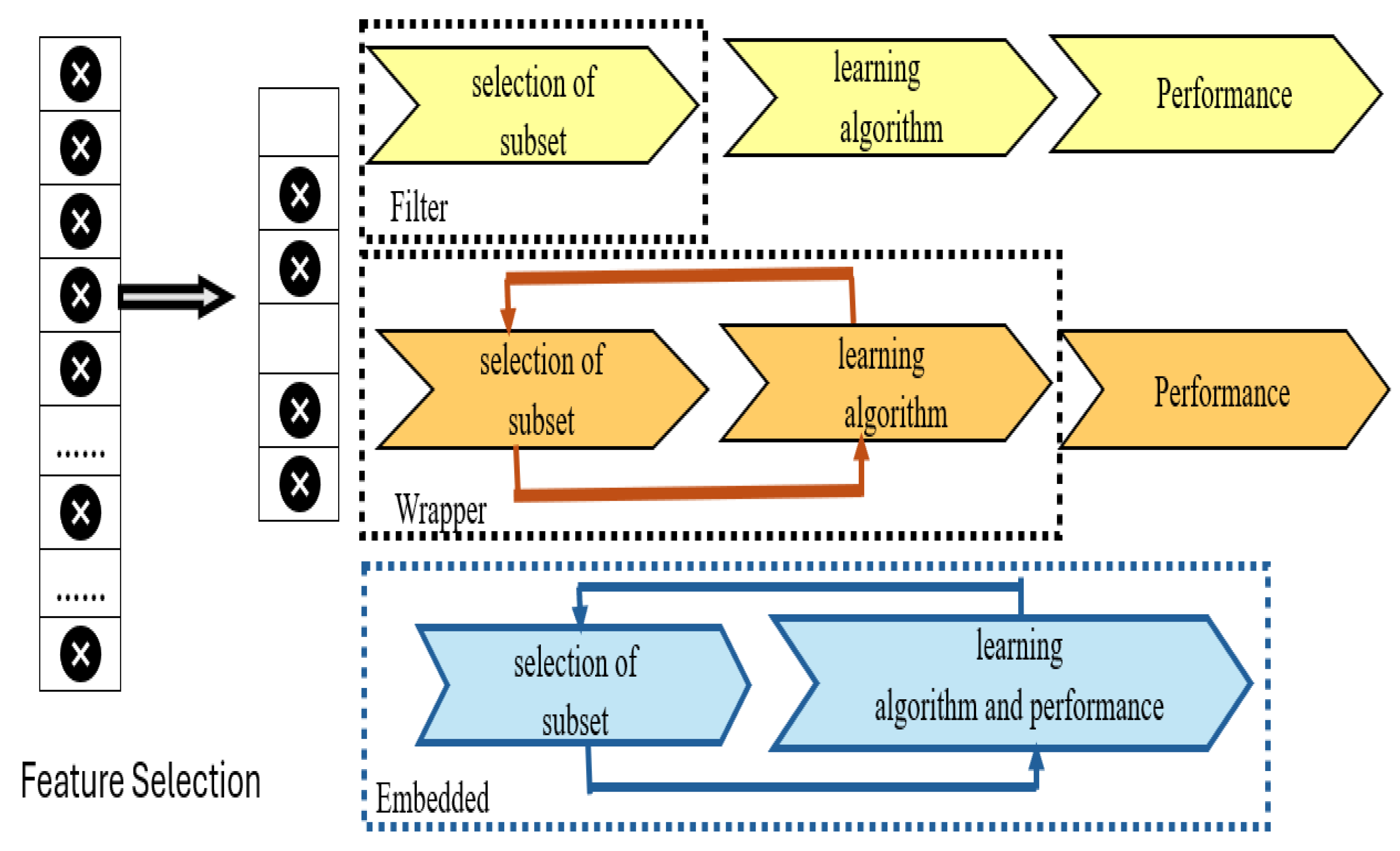
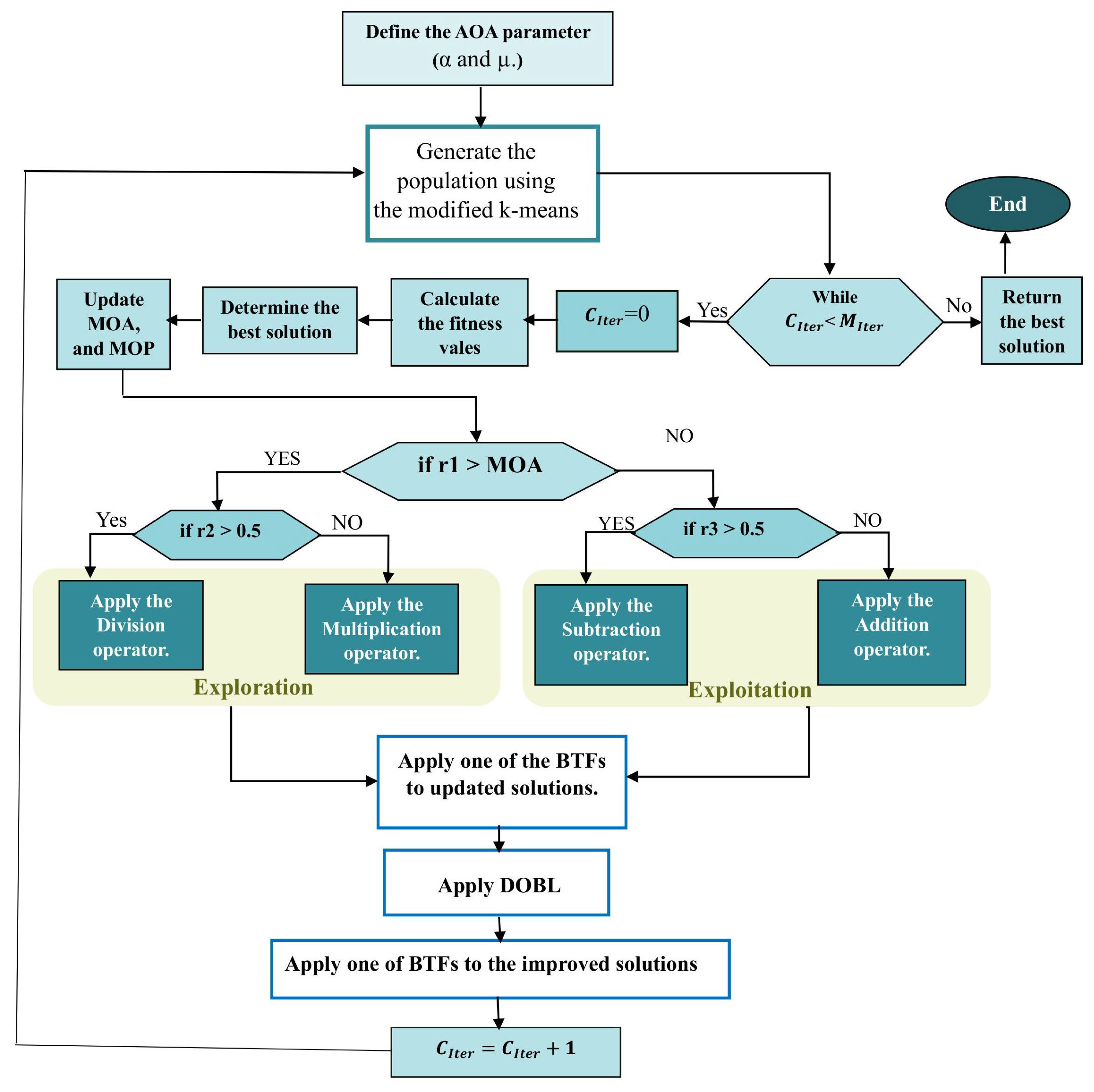
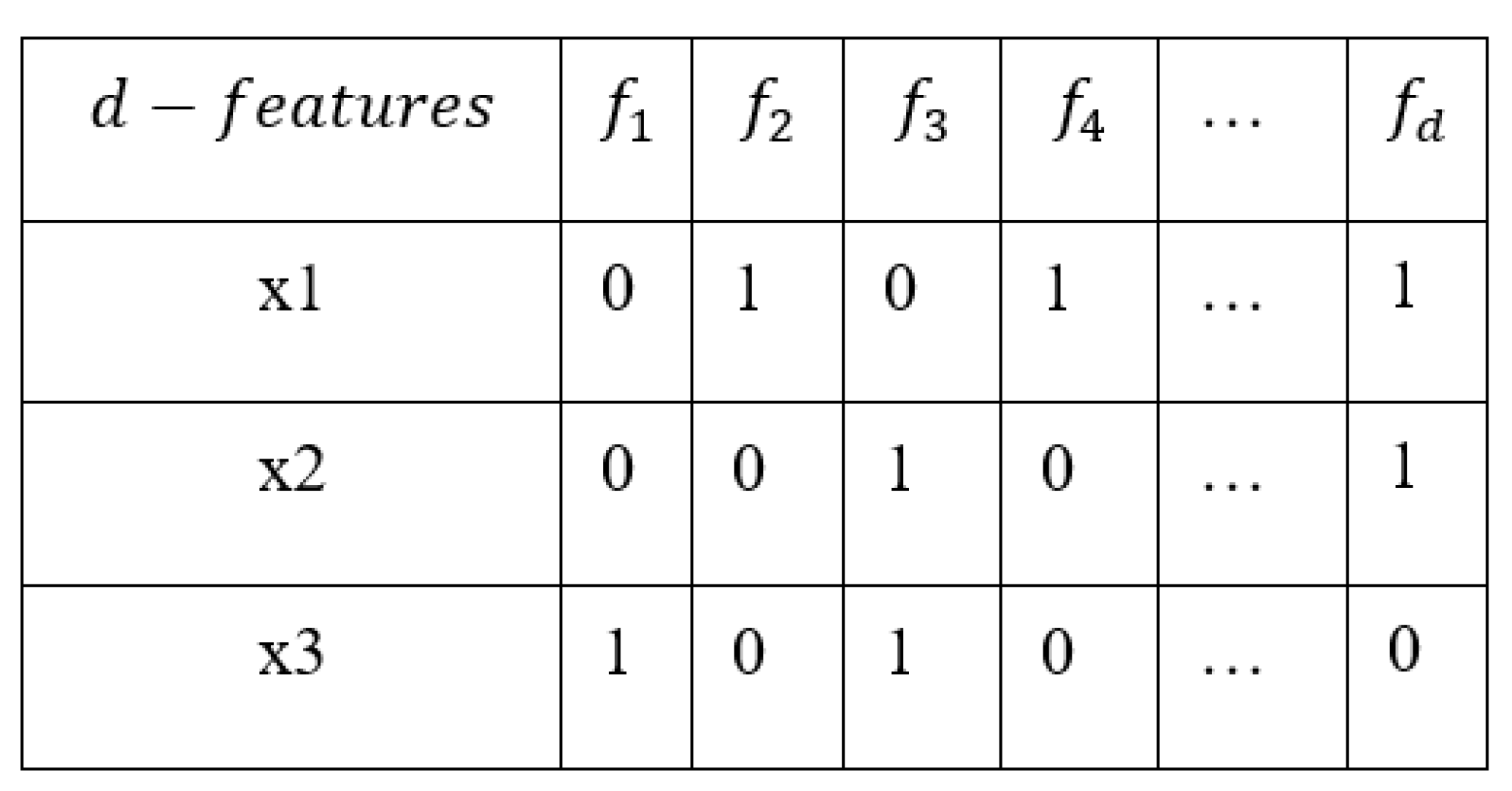

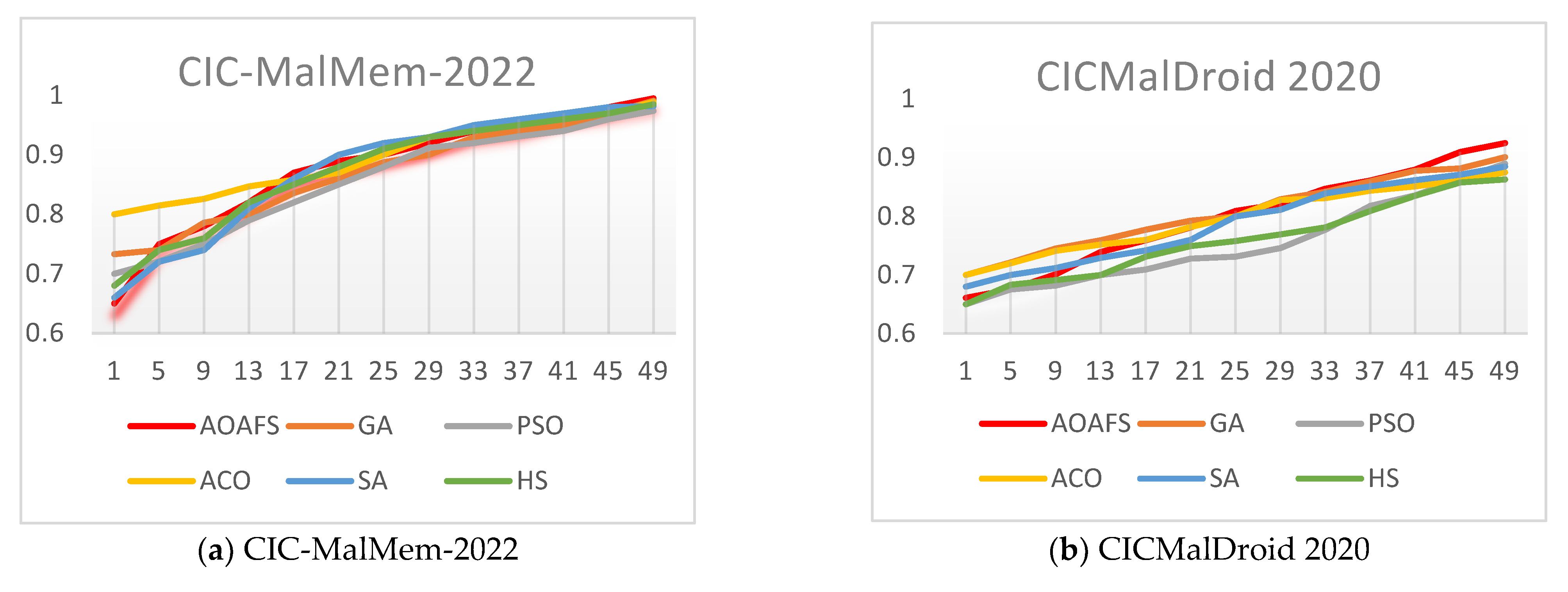
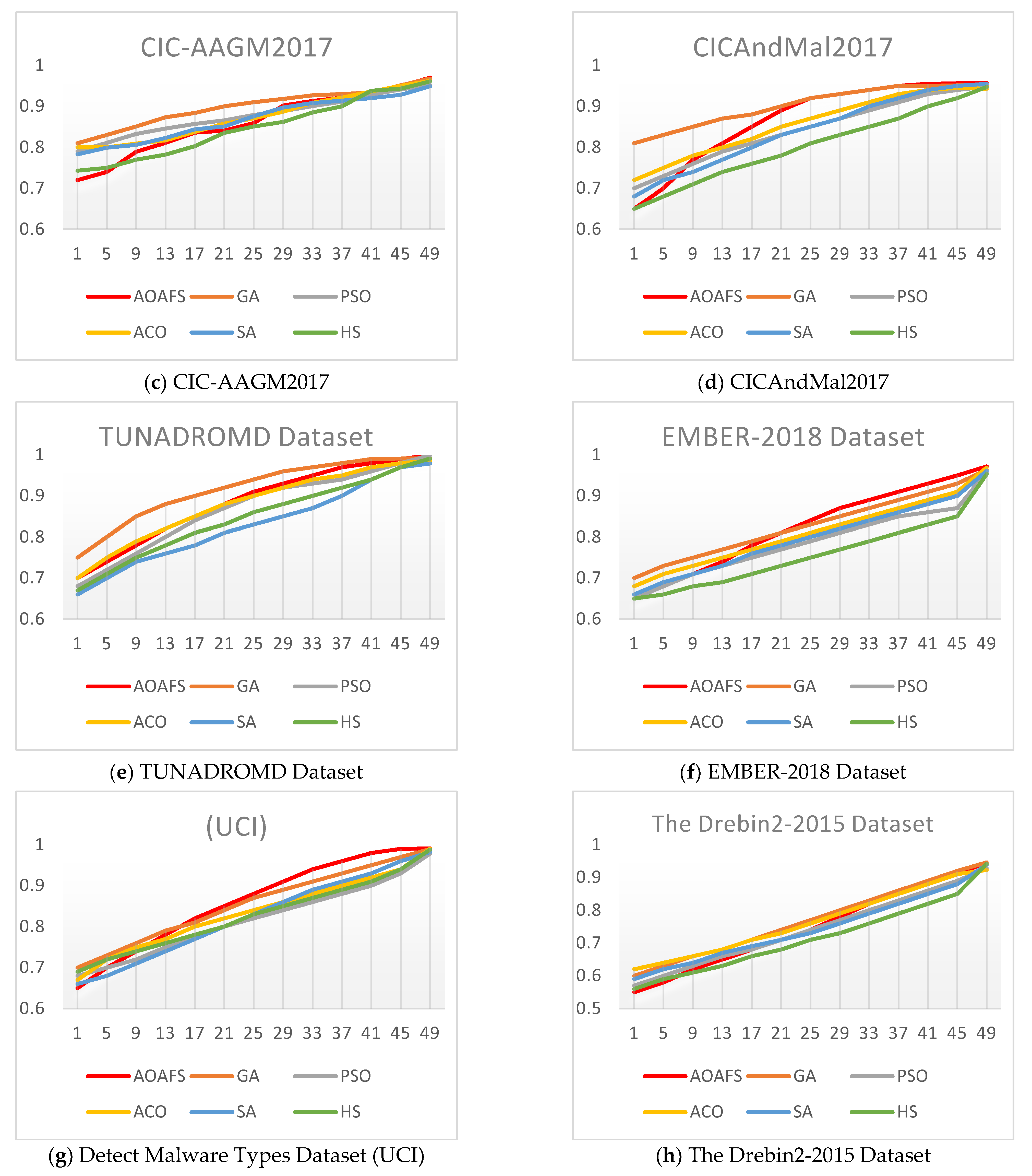
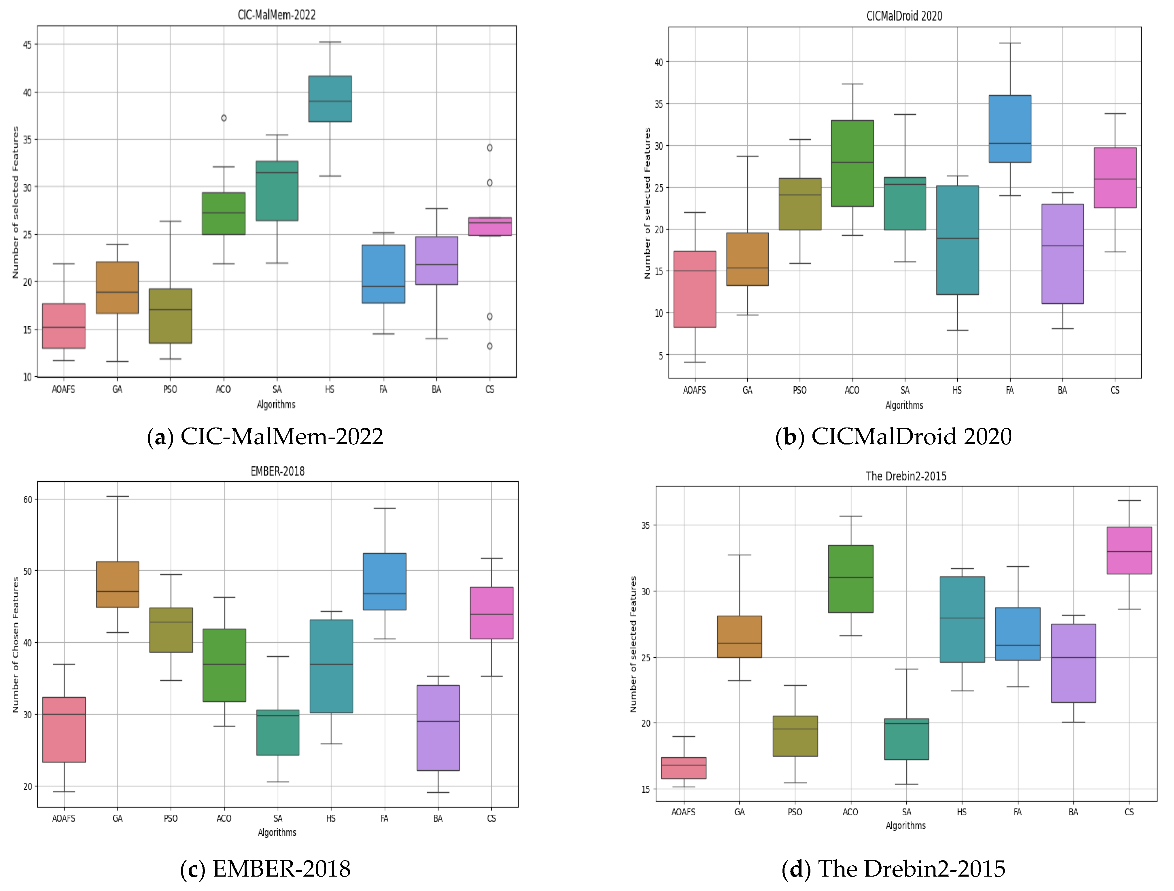
Disclaimer/Publisher’s Note: The statements, opinions and data contained in all publications are solely those of the individual author(s) and contributor(s) and not of MDPI and/or the editor(s). MDPI and/or the editor(s) disclaim responsibility for any injury to people or property resulting from any ideas, methods, instructions or products referred to in the content. |
© 2025 by the authors. Licensee MDPI, Basel, Switzerland. This article is an open access article distributed under the terms and conditions of the Creative Commons Attribution (CC BY) license (https://creativecommons.org/licenses/by/4.0/).