Abstract
This study examines whether portfolio optimization can be effectively based on annual changes in the harmonized index of consumer prices (HICP) data. Specifically, we assess whether asset allocation based on consumer expenditure can generate superior returns compared to static or equal-weighted asset allocation. To explore this, we use consumer expenditure data from HICP statistics categorized by COICOP. Our findings indicate that this strategy outperforms a buy-and-hold benchmark by 13.32% in terms of the Sharpe Ratio and exceeds an annual equal-weighted rebalancing strategy by 3.11%. Additionally, both the Calmar and Sterling Ratios demonstrate improved performance, further reinforcing the robustness of this approach. Furthermore, a hypothetical scenario where sector weights from the end of the given year—though not yet available during the year—are used suggests even greater improvements in performance. A high-sample bootstrap simulation confirms that the observed performance differences are not random but reflect the independent effectiveness of asset allocation based on consumer expenditure trends. This result strengthens the validity of our backtesting findings, indicating that the examined strategy could generate excess returns compared to passive portfolio managment and fixed-weight rebalancing approaches. The result of the study is therefore the development of an effective portfolio rebalancing strategy.
1. Introduction
Modern portfolio theory Markowitz (1952) paved the way in the field of risk measurement. This theory pioneered the combination of return and risk in equity investing. Lintner (1965), Mossin (1966), Sharpe (1966) and Treynor (1999) extended the model to other instruments. The theory points to the potential for risk reduction through diversification. Investing in a large number of stocks can reduce an investor’s risk relative to investing in individual stocks while increasing or maintaining returns. The variance proposed by Markowitz to measure risk is still used by many investors in practice (Bányai et al., 2024; Geboers et al., 2023).
The question arises as to what exactly the composition of an optimal portfolio should be, and whether the composition of the portfolio should be changed in the future. Portfolio management should provide answers to these questions. Portfolio management is the activity of making investment decisions in order to maximize the return on a portfolio of assets (Cooper et al., 1999; Ning et al., 2023). A number of portfolio management methods and techniques are presented in the literature, mainly based on quantitative investment. These methods range from the modern portfolio theory to traditional financial analysis methods (Amenc & Le Sourd, 2003). In this context, managers may choose different portfolio management approaches and styles depending on different factors such as investment objectives, risk profile and risk tolerance (Bender et al., 2009; Choi et al., 2024). They can choose a passive or active approach, a sector-oriented approach, a fundamental approach or a quantitative approach (Bulkley & Hashim, 2019). Each of these approaches has its own advantages and disadvantages and can have a significant impact on portfolio performance, costs and risk management and can be tailored to the needs of individual investors. According to the efficient market theory developed by Fama (1970), portfolio management can adopt a passive approach. According to this theory, it is impossible to outperform the market, as asset prices rapidly absorb new information that flows into the market. The passive approach relies on passively tracking a benchmark. Passive portfolio managers adopt a long-term investment strategy and try to replicate the performance of the benchmark portfolio without trying to outperform it. Diversification to reduce risk is an important element of passive management (Blackledge & Lamphiere, 2021).
A new approach, active portfolio management, has been developed to outperform passive management. In this approach, securities are selected on the basis of analysis with the aim of outperforming a benchmark index. Investment managers using this approach need to have a good understanding of financial markets and financial instruments and take into account the economic trends affecting financial markets. Therefore, the active approach requires the involvement of the portfolio manager, while the passive approach requires minimal involvement of the manager (Azouagh & Daui, 2023).
In our study, we take the approach that, if rebalanced appropriately, a portfolio can outperform if rebalancing is performed properly compared to if rebalancing is not performed. The asset portfolio is composed of ETFs that track the performance of different economic sectors. It is assumed that if we can allocate investments to sectors that outperform other sectors of the economy, then the portfolio can also outperform. The analysis is carried out for the euro area as a whole. The portfolio is reweighted on the basis of the change in final household consumption. The change in final consumption is derived from the change in the weights of the elements of the consumer basket used to calculate the HICP. The excess performance of the portfolio is evaluated using the Sharpe ratio, the Calmar ratio and the Sterling ratio.
2. Theoretical Background of the Study—Weights Used for Portfolio Rebalancing and Indicators Used to Measure Portfolio Performance
2.1. HICP Sub-Component Weights as Portfolio Weights
The Harmonised Index of Consumer Prices (HICP) is a measure of the change in consumer prices within the European Union (EU), reflecting the change over time in the prices of goods and services purchased by households. The basic aspect of the HICP is the use of a weighted basket of consumer goods, where the weight of each item represents its share in total consumption expenditure (Dietrich et al., 2021). These weights are key to the accurate calculation of the HICP, ensuring that the index reflects actual consumer spending patterns. The weights assigned to goods and services in the basket are essential to the accurate calculation of the HICP. They ensure that the index reflects actual consumer spending patterns and provides a reliable measure of inflation across the EU (European Commission, 2024).
We used the HICP/COICOP framework because it offers standardized and internationally comparable data on consumer spending patterns across EU Member States. These expenditure categories are consistently updated and reflect real household consumption behavior, making them a reliable proxy for underlying macroeconomic conditions. Their annual availability aligns well with the frequency of portfolio rebalancing in long-term investment strategies, ensuring both methodological consistency and economic relevance.
There are several steps in determining the weight of goods and services in the HICP.
The primary source of data for determining weights is the Household Budget Survey (HBS), which collects detailed information on household expenditure on different categories. In addition, national accounts data, in particular the Households Final Monetary Consumption Expenditure (HFMCE), provide a comprehensive insight into consumer expenditure. These data sources ensure that weights reflect actual consumption behavior (Statistisches Bundesamt, 2023).
Expenditure is categorized according to the Classification of Individual Consumption by Purpose (COICOP/HICP), which is adapted to the needs of the Harmonised Indices of Consumer Prices. This standardized classification facilitates a consistent grouping of similar items, which improves comparability between EU Member States. For each category, the share of total consumption expenditure is calculated. These ratios serve as an initial weight, indicating the relative importance of each category in the overall consumer basket. To maintain accuracy, these initial weights are adjusted to take account of price changes between the reference period and the reference period. This adjustment ensures that the weights reflect current price levels and consumption patterns. As consumer behavior and market conditions change, the weights are updated annually. This update includes the latest available data to reflect changes in consumption patterns.
Several sources are involved in determining and updating the HICP weights. These include the Household Budget Surveys (HBS), which provide detailed information on household expenditure as the basis for the calculation of weights. They use data from the National Accounts. HFMCE data from the National Accounts provide a comprehensive insight into overall consumer expenditure, complementing the detailed data from the HBS. The standardized COICOP/HICP classification. This standardized classification system ensures a consistent categorization of goods and services across EU Member States, facilitating comparability. The HICP subcomponents according of Classification of individual consumption by purpose (COICOP) are food and non-alcoholic beverages; alcoholic beverages, tobacco and narcotics; clothing; footwear; housing, water, electricity, gas and other fuels; furnishings, household equipment and routine household maintenance; health; transport; communications; recreation and culture; education; restaurants and hotels; and miscellaneous goods and services (Eurostat, n.d.).
The Harmonised Index of Consumer Prices (HICP) is therefore designed to take account of changing household consumption patterns through annual weight updates. The weights are updated at the beginning of each year. In line with the Laspeyres principle, these weights refer to the previous year’s expenditure and remain fixed throughout the year (European Commission, 2024).
Subcomponents are understood in this study as identifiable economic areas from an investment perspective. Therefore, we choose investment instruments that cover the relevant economic sectors. And for portfolio rebalancing, we use the variable subcomponent weights.
The factors determining investors’ portfolio decisions and financial instrument choices are diverse and closely related to financial market developments, the macroeconomic environment, and individual preferences. Classical economic approaches, in particular Tobin’s (1958) portfolio theory, have had a significant impact on the interpretation of portfolio choices. According to Tobin’s theory, investors construct their portfolios by taking into account individual risk aversion and establishing an optimal ratio between risky and risk-free assets. Tobin’s theory established the link between macro- and micro-level economic relationships.
As an extension of Markowitz’s (1952) expected return dispersion model, Tobin introduced the risk-free asset, which made it possible to adjust the so-called efficient frontier of portfolios. The modern portfolio theory based on this has become an important starting point for both financial economics and practical portfolio management.
Investors’ portfolio decisions may differ from theoretical models. Decisions are influenced by factors such as financial literacy (Li et al., 2020), age and housing needs (Pelizzon & Weber, 2009), access to credit markets (Duca & Muellbauer, 2013) or income uncertainty and the inflationary environment (Vukovic et al., 2022). Incorporating these factors into the Tobin model poses new theoretical and empirical challenges. However, the portfolio choices of individual investors do not influence which portfolios would be most appropriate in terms of risk–return optimization.
Our study is grounded in several key theoretical foundations that justify the use of consumer expenditure data in portfolio construction. It draws on core principles of Modern Portfolio Theory, integrates insights from Behavioral Finance regarding the relationship between spending behavior and economic sentiment, and reflects the logic of consumption-based asset pricing models (CCAPM) by linking expenditure patterns to asset allocation. Furthermore, the approach aligns with the principles of Adaptive Asset Allocation, emphasizing the dynamic adjustment of portfolios in response to macroeconomic signals.
In our study, we use the weights of the HICP subcomponents as the basis for our portfolio rebalancing strategy. This strategy has not been used in the investment strategies described in the literature to date. The strategy provides a novel approach to establishing excess returns for portfolios.
2.2. Indicators Used to Measure Portfolio Performance
2.2.1. Sharpe Ratio
The Sharpe Ratio is a widely used risk-adjusted performance metric introduced by Nobel laureate William F. Sharpe in 1966. It measures the excess return of an investment per unit of risk, where risk is defined as the standard deviation of returns. The ratio helps investors assess whether an asset or portfolio generates adequate returns relative to its volatility. The Sharpe Ratio is calculated by subtracting the risk-free rate of return, typically represented by government bonds, from the portfolio’s return and then dividing the result by the standard deviation of the portfolio’s returns (Sharpe, 1966).
A higher Sharpe Ratio indicates that an investment delivers greater excess return relative to its risk level, making it more attractive for risk-averse investors. Conversely, a lower Sharpe Ratio suggests that the returns may not sufficiently compensate for the risk taken. This metric is particularly useful in portfolio selection and performance evaluation, as it allows investors to compare different investments on a standardized risk–return basis (Gardenier et al., 2021). However, the Sharpe Ratio has certain limitations. It assumes that returns are normally distributed, which may not always hold true in real-world markets, and it does not distinguish between upside and downside volatility, potentially misrepresenting risk in non-linear markets. Despite these drawbacks, it remains the most widely used risk-adjusted performance metric in investment analysis and portfolio management (Beruticha et al., 2015; Sen, 2022).
2.2.2. Calmar Ratio
The Calmar ratio is a risk-adjusted performance metric introduced by fund manager Terry W. Young in 1991. It evaluates investment performance by comparing the compounded annual rate of return to the maximum drawdown over a specified period, typically the past 36 months. The formula is calculated by dividing the compounded annual return of an investment by its maximum drawdown (Young, 1994).
Compared to other risk-adjusted metrics, such as the Sharpe ratio, which evaluates return per unit of volatility, the Calmar ratio specifically focuses on drawdowns, making it particularly useful for investors concerned with capital preservation and downside risk management (Caporin & Lisi, 2011). A higher Calmar ratio indicates a more favorable risk-adjusted return, as it suggests that the investment generates strong returns while minimizing large losses. While the standard approach considers the maximum drawdown over a fixed period, some variations may adjust the calculation to incorporate rolling drawdowns or different time horizons, offering a more dynamic assessment of risk (Beyranvand et al., 2024) and (Sen, 2022).
2.2.3. Sterling Ratio
The Sterling ratio is another risk-adjusted performance measure, primarily used to evaluate hedge funds and investment portfolios. It assesses the return of an investment strategy relative to its average drawdown, providing insight into the efficiency of the strategy in managing downside risk. The formula is calculated by dividing the average annual return of an investment by the average drawdown (Kestner, 1996; Eling & Schuhmacher, 2007).
In this formula, a constant value (commonly 10%) is subtracted from the average drawdown to account for acceptable risk levels, reflecting the historical context when risk-free rates were around 10%. However, this constant is not mandatory in all cases, and the Sterling ratio can still serve as a useful risk-adjusted performance metric even without this adjustment. A higher Sterling ratio signifies a more favorable risk-reward profile, indicating that the investment yields higher returns relative to the expected level of risk. Compared to the Calmar ratio, which considers maximum drawdown, the Sterling ratio provides a broader view of risk by incorporating average drawdown, making it a useful alternative for evaluating investment strategies over extended periods (Almahdi & Yang, 2017; Arratia et al., 2022).
We chose this set of three performance metrics because they together offer a more comprehensive assessment of risk-adjusted returns. The Sharpe ratio captures return per unit of volatility, making it useful for evaluating overall efficiency. To complement this, the Calmar and Sterling ratios emphasize downside risk by focusing on drawdowns—an essential consideration in capital preservation. Nonetheless, both the Calmar and Sterling ratios have limitations: they are based on historical drawdowns, which may not fully reflect future risk exposures. The Calmar ratio considers only the maximum drawdown, potentially missing broader volatility, while the Sterling ratio can be influenced by the method used to calculate average drawdowns. For these reasons, we interpret them jointly to achieve a balanced understanding of portfolio performance.
3. Research Methodology
For this analysis, we used the Eurostat dataset (code: prc_hicp_inw), which provides annual consumer spending weights of euro area by COICOP categories from 1996 to 2024.
As a first step, we filtered the 12 available categories to exclude those for which no suitable investment fund could be identified. We focused on sectors where direct investment is feasible through the underlying companies represented in ETFs. For instance, sectors such as public education and healthcare are generally not directly investable via ETFs, as they are predominantly funded or operated by the public sector. Consequently, we concentrated exclusively on sectors for which a clear and precise mapping between COICOP categories and investable ETFs could be established. This selection was essential to ensure methodological consistency, avoid ambiguity in portfolio construction, and maintain the practical relevance of the strategy by relying solely on tangible, investable assets. The five selected COICOP categories account for approximately 59–60% of total household consumption in the Euro area, covering the majority of economically relevant and investable sectors. As a result, these categories were matched to iShares ETFs, each representing 600 companies within the corresponding sector. The real estate ETF (EXI5.DE) was matched to the COICOP category “Housing, water, electricity, gas and other fuels” as it covers core housing-related expenses. While the ETF targets property specifically, utilities are integral to real estate use and value, justifying their grouping under this category (Table 1).

Table 1.
Overview of assets and related COICOP categories included in the analysis. Source: own editing based on blackrock.com.
We chose iShares ETFs for two main reasons: first, to ensure consistency and easier comparability across sectors, and second, because analyzing a representative sector-based ETF provides a broader and more diversified exposure than individual stocks, which may carry country-specific risks. The examined period spanned from 4 January 2010, to 17 February 2025, covering a total of more than 15 years. The selected period was chosen with the explicit intention of capturing a comprehensive and representative range of economic conditions that could influence the examined variables. This timeframe includes the post-global financial crisis recovery, the European debt crisis, several monetary policy regime shifts (e.g., the introduction and eventual tapering of quantitative easing), the COVID-19 pandemic and its economic aftermath, as well as the recent global supply chain disruptions and energy price shocks. The data, published by Eurostat, is available on an annual basis, meaning that one rebalancing is possible each year based on the available COICOP weights. This means that during the examined period, the portfolio could be rebalanced each year.
During the examination, we set up a total of four scenarios. Two benchmarks were created, one of which represents a buy and hold strategy, where all five assets are purchased in equal proportions at the beginning of the examined period and the weights of the assets remain unchanged until the end of the period. The second benchmark refers to a portfolio where the weights also start in equal proportions, but rebalancing is applied once a year, resetting the weights to their original equal proportions. Thus, we created a passively and an actively managed portfolio, which will serve as a benchmark for measuring the relative performance of the assumed strategy. It is important to highlight that HICP consumer spending data are measured in the Euro area; hence, we selected only assets with geographical exposure to Europe to maintain consistency.
Subsequently, we created a portfolio similar to the previous one, where the initial weights are also equal. However, during the rebalancing periods, we always apply the weights based on the consumer spending from the previous year. This portfolio represents the actual backtesting of the strategy proposed in our study. Additionally, we simulated a portfolio in which rebalancing is performed using consumer spending data from the COICOP categories of the current year, rather than the previous year’s data. This scenario deliberately creates a hypothetical situation to test what would have happened if we had been able to use the COICOP category weights for the current year (which are only available a year later). With this scenario, we aim to assess whether applying future weights would provide an additional advantage compared to the previous approach (Table 2). After analyzing all possible scenarios, we identified March as the optimal rebalancing period, as our tests demonstrated that rebalancing during this month yielded the most favorable results across all scenarios. Consequently, for all scenarios, rebalancing is conducted on the last trading day of March.
Table 2.
Overview of scenarios analyzed. Source: own editing.
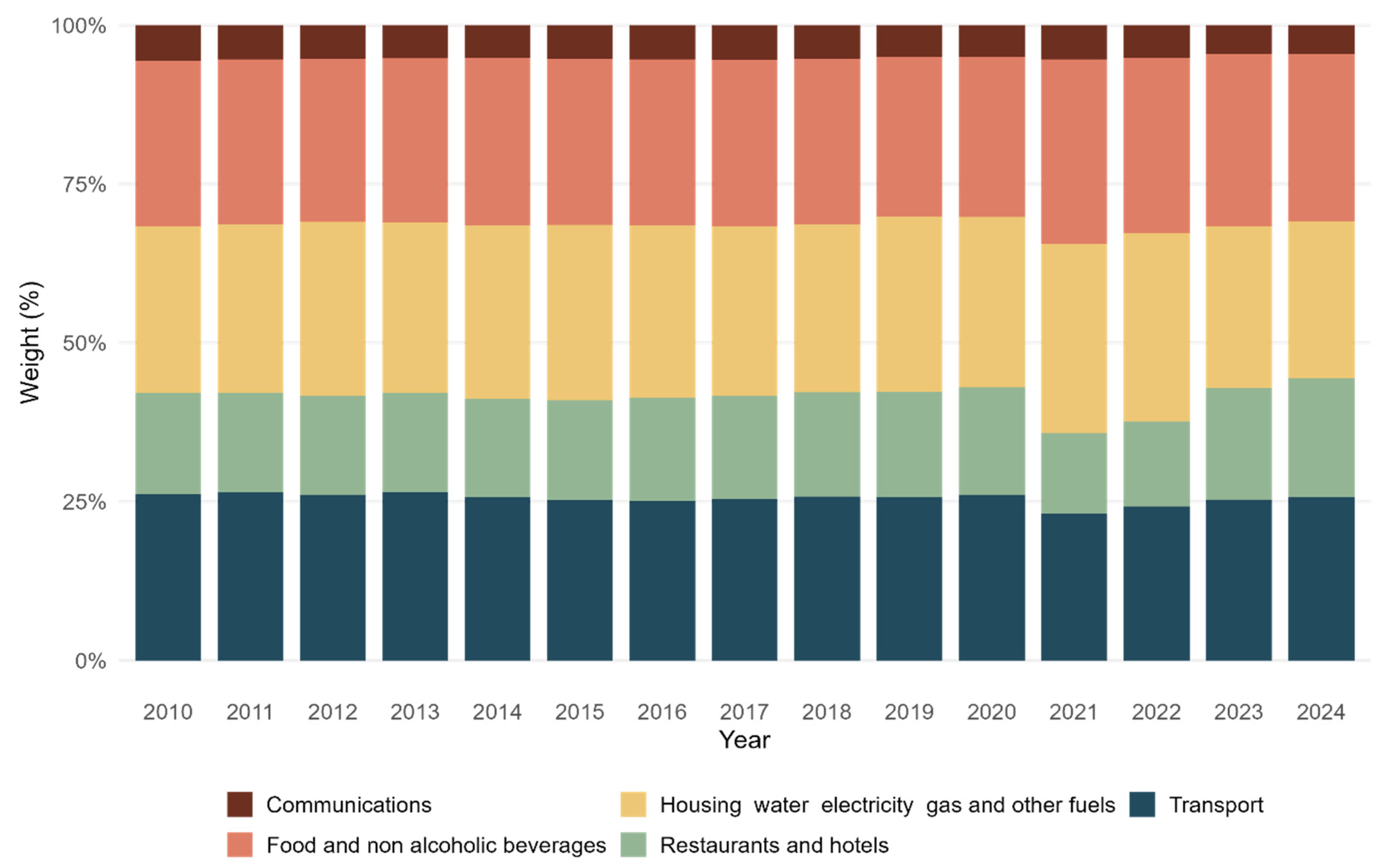
Between 2010 and 2024, the data show varying trends in consumer spending across categories. Food and non-alcoholic beverages experienced slight declines, with a notable increase in 2022, likely driven by inflation and supply chain disruptions caused by the COVID-19 pandemic. However, spending in this category decreased again in 2023 and 2024, suggesting potential stabilization in food prices or shifts in consumer preferences. Housing, water, electricity, gas, and other fuels saw a general increase in spending until 2022, followed by a decrease in 2023 and 2024, reflecting the effects of the energy crisis exacerbated by the Russian–Ukrainian conflict. The decline in recent years may also be attributed to energy market adjustments and reduced consumption due to higher efficiency measures.
Transport showed a dip in 2022 but began to recover in 2023 and 2024, likely due to shifting transportation preferences and changes in mobility patterns. Communications remained relatively stable with minimal fluctuations, though a slight decline in 2024 may indicate changing consumer habits or advancements in technology reducing costs. Restaurants and hotels experienced significant volatility, especially during the COVID-19 pandemic and its aftermath, with a strong recovery post-pandemic. The upward trend continued in 2024, reflecting increasing demand for hospitality and travel services. The Russian–Ukrainian conflict has had far-reaching effects on several categories, particularly energy prices and transportation, influencing consumer behavior and expenditure patterns. These changes underscore the impact of global crises, inflation, and political events on spending trends.
Before constructing portfolios, we could measure the correlation between consumer spending weights and the related average annual returns of the assets, but we face two problems. First, the sample size is relatively small, leading to high p-values, making it difficult to establish a statistically significant connection between the variables. Second, as seen in Figure 1, consumer spending weights are rather static, particularly in the first half of the period. Hence, relying solely on correlation analysis may not fully capture the dynamics between consumer expenditure patterns and asset performance. Even if we could establish a statistically significant connection, it would not necessarily translate into advantageous portfolio outcomes, as correlation alone does not imply profitability or superior risk-adjusted return. Instead, an appropriate way to test this is to construct portfolios and measure the compound effect of rebalancing based on consumer expenditure trends.
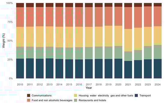
Figure 1.
Distribution of consumer spending as per selected COICOP categories from 2010 to 2024. Source: own editing based on ec.europa.eu/Eurostat.
To construct the portfolios analyzed, we built a deterministic model that performed simulation based on daily asset prices extracted from the Yahoo Finance database. In all cases, we used an initial investment of 1000 EUR with a 2% expected risk-free rate of return. The model followed a standard 252 trading day approach. To ensure a conservative estimate of net performance, we assumed a simplified 1% trading fee during rebalancing, acknowledging that actual transaction costs may vary across investor types. Each time a rebalancing event occurred, the daily gross portfolio return was adjusted by deducting trading fees, thus calculating the daily net portfolio return. Daily returns were calculated using the simple rate of return formula. To ensure a comprehensive performance comparison, we calculated not only standard KPIs such as net return and standard deviation but also the maximum and average drawdowns, as well as the Sharpe ratio, Calmar ratio, and Sterling ratio.
- 1.
- Sharpe Ratio
= expected return of the portfolio
= risk-free rate
= standard deviation of the portfolio
- 2.
- Calmar Ratio
= expected return of the portfolio
= risk-free rate
Maximum Drawdown = the greatest peak-to-trough decline in the portfolio’s value over a specific period
- 3.
- Sterling Ratio
= expected return of the portfolio
= risk-free rate
Average Drawdown = the average of all drawdowns over a specific period
In addition to the previously discussed indicators, the simulation also focused on two key measures: Net Portfolio Value (NPV) and Net Portfolio Return (NPR). These metrics were used to quantify the overall value generated by the strategies and to assess their performance on a net basis.
- 4.
- Net Portfolio Value (NPV)
= the net portfolio value at time
= the price of asset at time
= the number of units held of asset at time
= the total number of assets in the portfolio
- 5.
- Net Portfolio Return (NPR)
= the net portfolio return at time
= the net portfolio value at time
= the net portfolio value at time
4. Results
4.1. Descriptive Statistics
In this section, we will present a descriptive analysis (Table 3) of the assets analyzed in the portfolio simulation.
Table 3.
Descriptive statistics of simple returns. Source: own editing.
The five assets show varied risk–return profiles, as indicated by their average return and standard deviation. EXV5.DE stands out with the highest average return of 11.80%, but this comes with a relatively high standard deviation of 26.66%, suggesting a higher level of volatility compared to the other assets. In contrast, EXH3.DE offers a more moderate average return of 7.38%, with a lower standard deviation of 14.37%, indicating a more stable performance. EXI5.DE has an average return of 5.46% and a higher standard deviation of 19.64%, indicating some level of risk, but with less return than EXH3.DE. EXV2.DE, with the lowest average return of 4.17%, also demonstrates a moderately high standard deviation of 16.72%. EXV9.DE offers an average return of 9.71% with a standard deviation of 22.18%, showing a balanced profile between risk and return. If we check the ratio of average return to standard deviation, EXH3.DE had the highest risk-adjusted return (0.5136), while EXV2.DE had the lowest (0.2495), which means that EXH3.DE offered the most efficient return relative to its volatility, whereas EXV2.DE delivered the least favorable risk–return trade-off among the analyzed ETFs.
In terms of skewness, all assets show negative values, which suggests that their returns tend to have a longer left tail, meaning they are more prone to negative extreme values than positive ones. The most pronounced negative skewness is observed in EXH3.DE (−0.4200), implying a greater likelihood of downside risk compared to the other assets. The kurtosis values, which measure the “tailedness” of the return distribution, are quite high for all assets, particularly for EXV2.DE (8.1211). High kurtosis values indicate that the return distributions of these assets exhibit a greater frequency of extreme values (both positive and negative) compared to a normal distribution, suggesting higher risk in terms of large fluctuations. Overall, these assets offer varied trade-offs between return and risk, with negative skewness and high kurtosis, indicating potential outliers. Despite their negative skewness and high kurtosis, these assets remain feasible in optimization due to their diversification potential. Optimization considers the overall portfolio’s risk–return profile, not just individual asset distributions. As such, they can serve as valuable candidates for portfolio optimization.
4.2. Correlation Matrix
Following the descriptive statistics, we constructed a correlation matrix (Table 4) for the asset yields.
Table 4.
Correlation matrix of the returns of the instruments. Source: own editing.
The correlation matrix reveals that all five assets exhibit positive correlations with each other, indicating that their returns generally move in the same direction. This suggests that when one asset performs well, the others are likely to follow suit. The correlations are statistically significant, with all p-values being less than 0.001. The highest correlation is between EXH3.DE and EXV2.DE (0.6413), indicating a strong relationship between these two assets. The positive correlations with other assets are moderate (EXI5.DE: 0.5946, EXV5.DE: 0.5447, EXV9.DE: 0.5717), signaling that EXH3.DE shares consistent return patterns with the others, although the relationship is stronger with EXV2.DE.
Similarly, EXI5.DE shows moderate positive correlations with all the other assets, especially with EXV9.DE (0.6348) and EXV5.DE (0.5843), indicating that it moves in sync with the others to a lesser extent. EXV5.DE and EXV9.DE exhibit the highest correlation with each other (0.6631), meaning their returns are highly synchronized. While these positive correlations suggest that the assets will likely produce similar returns, they may offer limited diversification benefits if included together in a portfolio. Nevertheless, their varying degrees of correlation provide an opportunity to diversify risk, as they do not perfectly mirror each other’s movements. This insight is valuable for portfolio construction, as combining these assets strategically could help achieve a balanced risk–return profile.
4.3. Simulation Results
To analyze and compare the performance of the constructed portfolios, we will present trend analysis (Figure 2) and summary statistics, including the average return, standard deviation (volatility), maximum and average drawdown, as well as three key KPIs: the Sharpe ratio, Calmar ratio, and Sterling ratio (Table 5). We will also analyze the distribution of relative portfolio value differences to reveal the detailed effect of the different strategies (Figure 3). Additionally, we will further examine the results using bootstrap simulation.
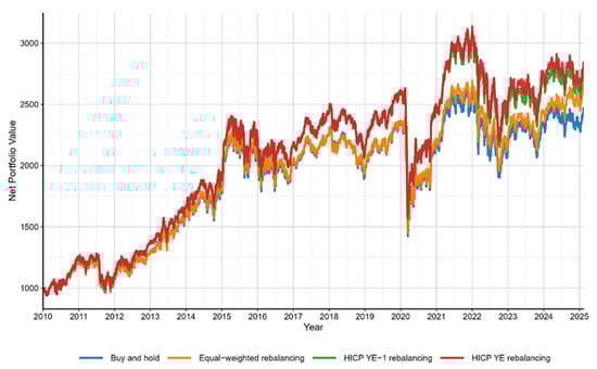
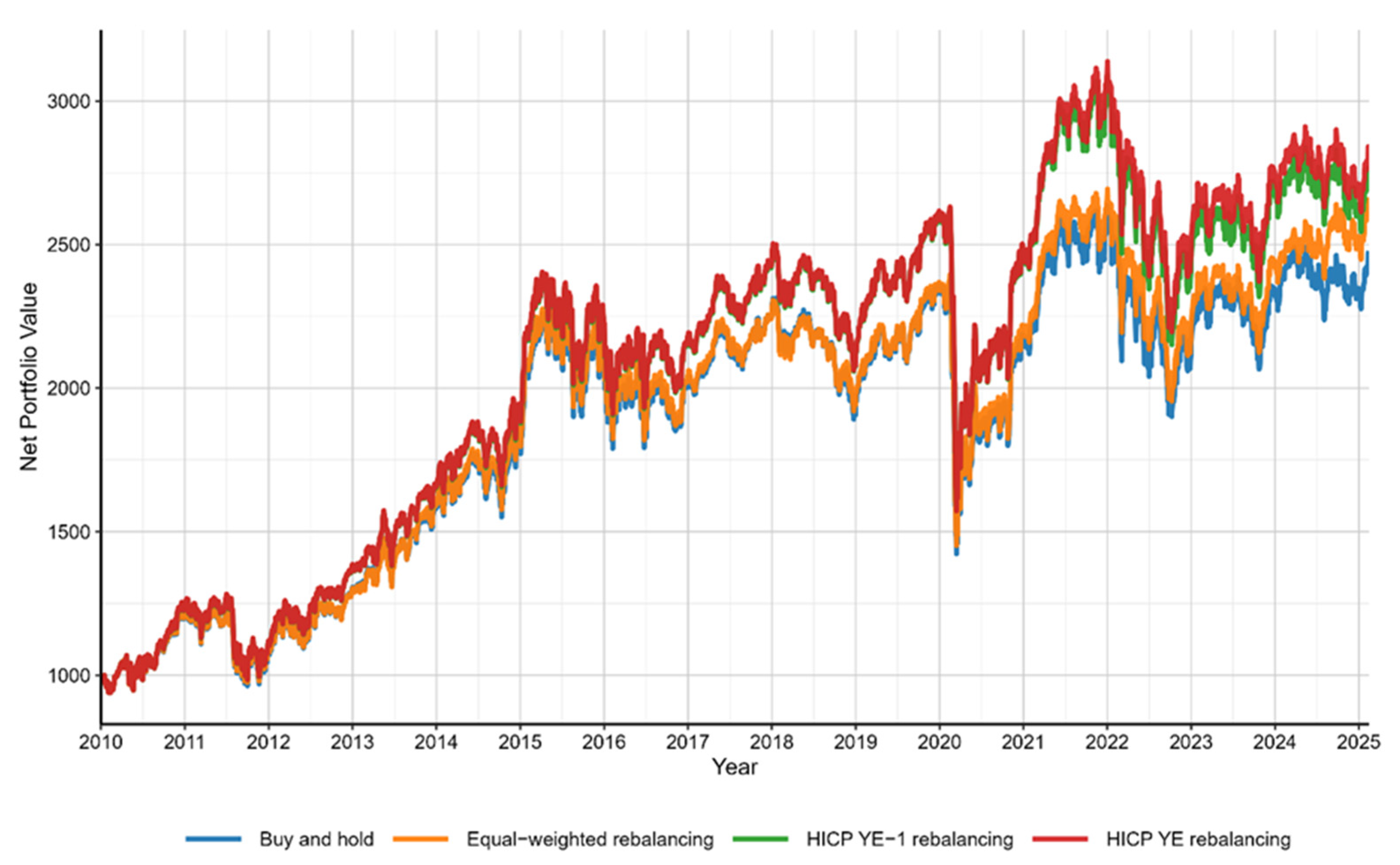
Figure 2.
Net portfolio values across different scenarios. Source: own editing.
Table 5.
Summary of performance metrics for the analyzed portfolios. Source: own editing.
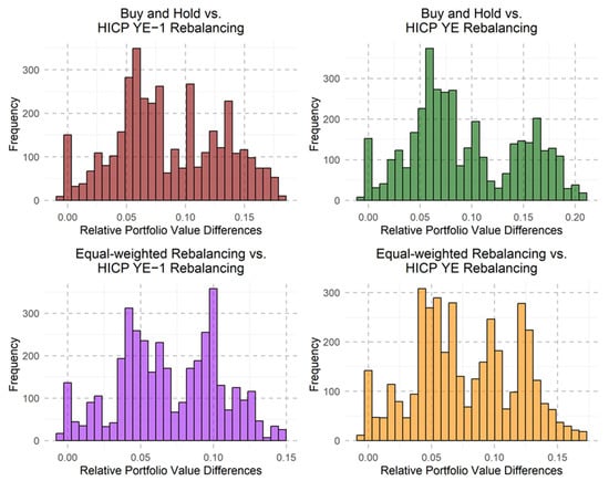
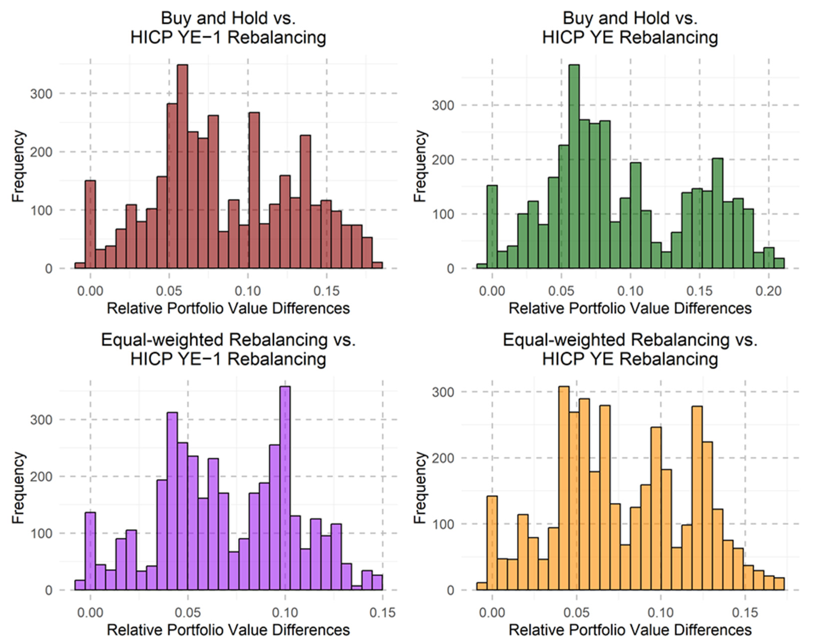
Figure 3.
Distribution of relative portfolio value differences. Source: own editing.
Over the 15-year period from 2010 to 2025, the buy and hold and equal-weighted rebalancing portfolios, acting as benchmarks, consistently showed growth (Figure 2). The buy and hold portfolio increased from 1054.97 to 2369.33, while the equal-weighted rebalancing portfolio grew from 1056.29 to 2551.42, demonstrating stable returns throughout the years. These two portfolios were based on more passive strategies: buy and hold maintained a constant position, and equal-weighted rebalancing periodically rebalanced the weights. On the other hand, the two strategies we tested—HICP YE−1 rebalancing and HICP YE rebalancing—yielded higher returns, with the HICP YE rebalancing portfolio achieving the greatest growth, reaching 2727.26 by 2025. Both of these tested strategies exceeded the performance of the benchmarks, reflecting the effectiveness of incorporating inflation-adjusted rebalancing approaches.
The overall performance trend shows that while the buy and hold and equal-weighted rebalancing benchmarks steadily grew over the years, the HICP YE−1 rebalancing and HICP YE rebalancing strategies delivered superior returns, particularly from 2021 onwards, when their portfolio values peaked at 3114.87 and 3069.75, respectively. These strategies demonstrated higher growth potential due to their inflation-sensitive adjustments, which helped them outperform the benchmarks during periods of higher inflation. However, while the tested strategies showed more pronounced peaks in value, the buy and hold and equal-weighted rebalancing portfolios remained solid performers, offering a more stable and consistent growth trajectory. Overall, the strategies we tested proved to be effective in generating higher returns, which supports our research question regarding the potential effectiveness of building rebalancing strategies based on consumer expenditure data.
Over the observed period (Table 5), the buy and hold portfolio showed a net return of 7.34%, while the equal-weighted rebalancing portfolio slightly outperformed it with a return of 7.77%. Both portfolios exhibited stable performance with relatively low volatility, as reflected by their standard deviations of 16.63% for buy and hold and 16.34% for equal-weighted rebalancing. The equal-weighted rebalancing strategy also showed a lower maximum drawdown (39.41%) compared to the buy and hold portfolio (40.11%), suggesting a slightly lower risk profile and a greater ability to limit losses during market downturns. Additionally, the average drawdowns were similar between the two portfolios, with buy and hold having an average drawdown of 7.83% and equal-weighted rebalancing slightly lower at 7.34%, indicating both strategies experienced similar loss patterns during market corrections.
The HICP YE−1 rebalancing and HICP YE rebalancing portfolios showed superior performance in terms of returns. The HICP YE rebalancing portfolio achieved the highest return at 8.29%, closely followed by the HICP YE−1 rebalancing portfolio with 8.12%. These two strategies also had higher sharpe ratios, with HICP YE rebalancing leading at 0.3752, indicating better risk-adjusted returns compared to the benchmarks. Despite slightly higher maximum drawdowns in both portfolios (40.07% for HICP YE−1 and 40.25% for hicp ye), their higher returns and stronger sharpe ratios indicate their effectiveness in achieving better overall performance. In terms of risk-adjusted performance, the HICP YE−1 rebalancing and HICP YE rebalancing portfolios showed better results on both the calmar and sterling ratios. The HICP YE rebalancing portfolio had the highest calmar ratio (0.1564) and sterling ratio (0.8027), reinforcing its strong performance relative to the risk involved.
Overall, HICP YE−1 rebalancing outperformed both benchmarks across nearly all metrics, surpassing both the buy and hold and equal-weighted rebalancing strategies. The Sharpe ratio increased by 13.32% compared to buy and hold and by 3.11% relative to equal-weighted rebalancing, while the Calmar ratio saw even stronger improvements of 14.69% and 4.33%, respectively. However, the Sterling ratio showed a 12.48% increase over buy and hold but declined by 2.43% compared to equal-weighted rebalancing. These findings are further reinforced by HICP YE rebalancing, which delivered even stronger improvements over HICP YE−1 rebalancing, with gains of 3.04% in the Sharpe ratio, 2.38% in the Calmar ratio, and 4.60% in the Sterling ratio. This confirms that the results from HICP YE−1 rebalancing were not coincidental, as even greater improvements were observed when using future year-end data instead of the historical data available at the time of rebalancing. This further supports the effectiveness of allocating assets based on consumer spending patterns in the analyzed sample.
To evaluate the deviations from the benchmark, we analyzed the distribution of relative portfolio value differences across four strategies (Figure 3). HICP YE−1 rebalancing vs. buy and hold shows the highest mean (0.0933) and 3rd quartile (0.1435), indicating that the strategy generally outperforms the benchmark, especially at the higher end of the distribution. With a maximum value of 0.2098, this strategy also demonstrates the potential for significant positive returns. However, the standard deviation of 0.0527 highlights the higher volatility associated with this strategy, suggesting that the returns are more variable compared to the others. The HICP YE−1 strategy shows slight positive skewness (0.1245), indicating a mild tendency for higher-than-average net portfolio values. However, due to its low magnitude and the large sample size, this is more likely the result of random variation than a structural pattern. This is supported by the negative kurtosis (−0.8288), indicating fewer extreme outcomes than in a normal distribution.
Next, HICP YE rebalancing vs. buy and hold follows with a mean of 0.0854 and a 3rd quartile of 0.1235, demonstrating strong performance, though slightly below the HICP YE−1 rebalancing vs. buy and hold strategy. The standard deviation of 0.0450 suggests moderate variability in the portfolio’s returns. The negative skew of −0.0637 implies that the majority of the values are clustered around the median, with fewer extreme positive outliers. The kurtosis of −0.7390 also suggests that this distribution has fewer extreme deviations compared to a normal distribution, indicating more consistency in returns.
When comparing HICP YE−1 rebalancing vs. equal-weighted rebalancing and HICP YE rebalancing vs. equal-weighted rebalancing, the former shows a mean of 0.0854, with a 3rd quartile of 0.1235, slightly trailing HICP YE−1 rebalancing vs. buy and hold, but still indicating solid performance. The standard deviation of 0.0450 suggests moderate variability in the portfolio’s returns. The negative skew of −0.0637 implies that the majority of the values are clustered around the median, with fewer extreme positive outliers. The kurtosis of −0.7390 also suggests that this distribution has fewer extreme deviations compared to a normal distribution.
Finally, HICP YE rebalancing vs. equal-weighted rebalancing shows the lowest mean of 0.0697, accompanied by the smallest standard deviation of 0.0349, pointing to the most consistent, yet less aggressive, performance of the four strategies. The negative skew of −0.0637 in this case suggests a more balanced distribution, with a tendency toward slightly lower relative performance. With a kurtosis of −0.7390, this strategy demonstrates fewer extreme deviations from the mean, reinforcing its steadier performance. The overall distribution indicates that, while this strategy is stable, it may not capture the higher positive deviations seen in other strategies, offering a more conservative risk–return tradeoff.
To further validate the results, we conducted a bootstrap simulation with 100,000 iterations, using resampling techniques to generate multiple portfolio scenarios. The analysis was also tested with lower iteration counts, yielding consistent results. The simulation leveraged the net values of the constructed portfolios and applied a 99% confidence interval to assess the reliability of the outcomes. The simulated average values of the portfolios, as shown in Figure 4, closely align with the deterministic results, reinforcing the reliability and robustness of the strategy. The low correlation coefficients from the bootstrap simulations (Table 6), suggest that the strategies behave independently, reflecting their fundamentally different rebalancing mechanisms—static rules in benchmark strategies versus dynamic adjustment in HICP-based ones. This structural difference, confirmed by narrow bootstrap confidence intervals, explains the weak correlation. This suggests that the observed performance differences are not due to randomness but reflect the actual, independent effectiveness of each strategy. Therefore, the previously observed superior performance of HICP YE-1 and HICP YE rebalancing relative to the benchmark is not due to randomness, but reflects a consistent, distinct advantage in its strategy that is linked to asset allocation based on consumer expenditure trends.
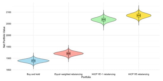
Figure 4.
Violin plot of bootstrap simulation at 99% confidence interval. Source: own editing.
Table 6.
Correlation matrix of portfolio net values based on the bootstrap simulation at a 99% confidence interval. Source: own editing.
5. Conclusions
Based on our research findings, it has been demonstrated that asset allocation based on consumer expenditure trends can generate superior risk-adjusted returns compared to static or equal-weighted rebalancing strategies. Our findings indicate that such a strategy not only outperforms the buy-and-hold benchmark by 13.32% in terms of Sharpe ratio but also exceeds an annual equal-weighted rebalancing strategy by 3.11%. Additionally, the strategy achieved a 14.69% improvement in the Calmar ratio and a 12.48% increase in the Sterling ratio compared to the buy-and-hold benchmark. When compared to the equal-weighted rebalancing strategy, it demonstrated a 4.33% higher Calmar ratio, while the Sterling ratio showed a slight decline of 2.43%. These results confirm that incorporating consumer expenditure data into portfolio construction can enhance performance by aligning asset weights with evolving spending patterns.
The bootstrap simulation further validated our findings by confirming that the observed performance differences are not random but reflect the independent effectiveness of the asset allocation strategy. The results of 100 000 iterations demonstrated consistent outperformance of HICP-based rebalancing strategies compared to both benchmarks, reinforcing the robustness of the proposed approach. Additionally, the low correlation coefficients between the bootstrap simulations suggest that the strategies operate independently, further supporting the conclusion that the superior performance is not due to chance but rather an inherent advantage of aligning asset allocation with consumer expenditure.
Overall, our research underscores the viability of an HICP-based asset allocation strategy and highlights its potential as a superior alternative to static and equal-weighted approaches. Future research could further refine this strategy by exploring more granular expenditure categories, extending the dataset, or integrating additional macroeconomic factors to enhance predictability and effectiveness in portfolio management. By leveraging sector-specific consumer expenditure data, investors can optimize their portfolios in a manner that is more responsive to real-world economic conditions, potentially enhancing returns while maintaining risk control. Additionally, analyzing different rebalancing frequencies (e.g., monthly or other periodic adjustments) could further refine the approach and uncover additional benefits and potential enhancements in this type of portfolio optimization.
While the proposed approach provides a novel framework for linking consumer expenditure patterns to portfolio strategies, certain methodological considerations merit further attention. The annual availability of HICP data limits rebalancing flexibility, and the COICOP system’s limited granularity and geographic extensibility may affect the precision of ETF mapping. Additionally, while ETFs serve as practical proxies for consumer expenditure categories, in some cases their composition may reflect firm-level or regional characteristics that slightly diverge from aggregate consumption trends. The use of lagged expenditure weights also constrains real-time applicability. Furthermore, while the model demonstrates improved performance, it does not test for causal relationships between consumption patterns and asset returns. Future research could address these limitations by incorporating more granular and frequent expenditure data, enhancing ETF mapping techniques, and exploring potential lead-lag relationships and causal links. The use of a deterministic model ensured practical interpretability, but future research could consider stochastic approaches, such as Monte Carlo simulations, to capture uncertainty and assess probabilistic outcomes.
Author Contributions
Conceptualization, A.B., L.P., and G.T.; methodology, A.B., L.P., and T.T.; validation, L.P., and T.T.; writing—original draft preparation, A.B., T.T., and L.P.; visualization, A.B.; supervision, L.P., and T.T. All authors have read and agreed to the published version of the manuscript.
Funding
This research received no external funding.
Institutional Review Board Statement
Not applicable.
Informed Consent Statement
Not applicable.
Data Availability Statement
The data presented in this study are available on request from the corresponding author.
Conflicts of Interest
The authors declare no conflicts of interest.
References
- Almahdi, S., & Yang, S. Y. (2017). An adaptive portfolio trading system: A risk-return portfolio optimization using recurrent reinforcement learning with expected maximum drawdown. Expert Systems with Applications, 87, 267–279. [Google Scholar] [CrossRef]
- Amenc, N., & Le Sourd, V. (2003). Portfolio theory and performance analysis. In The wiley finance series. Wiley. [Google Scholar]
- Arratia, A., Gzyl, H., & Mayoral, S. (2022). Tracking a well diversified portfolio with maximum entropy in the mean. Mathematics, 10(4), 557. [Google Scholar] [CrossRef]
- Azouagh, I., & Daui, D. (2023). Comparative analysis of active and passive portfolio management: A theoretical approach. International Journal of Accounting, Finance, Auditing, Management and Economics, 4(3-1), 504–517. [Google Scholar]
- Bányai, A., Tatay, T., Thalmeiner, G., & Pataki, L. (2024). Optimising portfolio risk by involving crypto assets in a volatile macroeconomic environment. Risks, 12(4), 68. [Google Scholar] [CrossRef]
- Bender, J., Briand, R., Nielsen, F., & Stefek, D. (2009). Portfolio of risk premia: A new approach to diversification. MSCI Barra Research Paper, 2009, 1–13. [Google Scholar] [CrossRef]
- Beruticha, J. M., López, F., Luna, F., & Quintana, D. (2015). Robust technical trading strategies using GP for algorithmic portfolio selection. Expert Systems with Applications, 46, 307–315. [Google Scholar] [CrossRef]
- Beyranvand, M., Davoodi, S. M. R., & Sharifi-Ghazvini, M. (2024). Distributionally Robust portfolio Optimization based on the Calmar ratio using the Wasserstein metric. International Journal of Finance & Managerial Accounting, 11(40), 81–92. [Google Scholar]
- Blackledge, J., & Lamphiere, M. (2021). A review of the fractal market hypothesis for trading and market price prediction. Mathematics, 10(1), 117. [Google Scholar] [CrossRef]
- Bulkley, K. E., & Hashim, A. K. (2019). Portfolio management models. In Handbook of Research on School Choice (pp. 302–316). Routledge. [Google Scholar]
- Caporin, M., & Lisi, F. (2011). Comparing and selecting performance measures using rank correlations. Economics, 5(1), 20110010. [Google Scholar] [CrossRef]
- Choi, J., Kim, H., & Kim, Y. S. (2024). Diversified reward-risk parity in portfolio construction. Studies in Nonlinear Dynamics & Econometrics, 17(2), 167–177. [Google Scholar]
- Cooper, R. G., Edgett, S. J., & Kleinschmidt, E. J. (1999). New product portfolio management: Practices and performance. Journal of Product Innovation Management: An International Publication of The Product Development & Management Association, 16(4), 333–351. [Google Scholar]
- Dietrich, A., Eiglsperger, M., Mehrhoff, J., & Wieland, E. (2021). Chain linking over December and methodological changes in the HICP: View from a central bank perspective (No. 40). In ECB Statistics Paper. European Central Bank. [Google Scholar]
- Duca, J., & Muellbauer, J. (2013). Tobin LIVES: Integrating evolving credit market architecture into flow of funds based macro-models No. (1581). In ECB Working Paper. European Central Bank. [Google Scholar]
- Eling, M., & Schuhmacher, F. (2007). Does the choice of performance measure influence the evaluation of hedge funds? Journal of Banking & Finance, 31(9), 2632–2647. [Google Scholar]
- European Commission. (2024). Harmonised Index of Consumer Prices (HICP) methodological manual (2024 edition). Publications Office of the European Union. [Google Scholar]
- Eurostat. (n.d.) HICP methodology. Available online: https://ec.europa.eu/eurostat/web/hicp/methodology (accessed on 3 December 2024).
- Fama, E. F. (1970). Efficient capital markets: A review of theory and empirical work. The Journal of Finance, 25(2), 383–417. [Google Scholar] [CrossRef]
- Gardenier, J., Lac, V., & Ashfaq, M. (2021). Risk-adjusted return in sustainable finance: A comparative analysis of European positively screened and best-in-class ESG investment portfolios and the Euro Stoxx 50 index using the Sharpe Ratio. In IUBH Discussion Papers—Business & Management No. 7/2021. IU Internationale Hochschule. [Google Scholar]
- Geboers, H., Depaire, B., & Annaert, J. (2023). A review on drawdown risk measures and their implications for risk management. Journal of Economic Surveys, 37(3), 865–889. [Google Scholar] [CrossRef]
- Kestner, L. N. (1996). Getting a handle on true performance. Futures, 25(1), 44–46. [Google Scholar]
- Li, J., Li, Q., & Wei, X. (2020). Financial literacy, household portfolio choice and investment return. Pacific-Basin Finance Journal, 62, 101370. [Google Scholar] [CrossRef]
- Lintner, J. (1965). The valuation of risk assets and the selection of risky investments in stock portfolios and capital budgets. Review of Economics and Statistics, 47, 13–37. [Google Scholar] [CrossRef]
- Markowitz, H. (1952). Portfolio selection. Journal of Finance, 7, 77–91. [Google Scholar]
- Mossin, J. (1966). Equilibrium in a capital asset market. Econometrica, 34, 768–783. [Google Scholar] [CrossRef]
- Ning, Y., Yang, S., & Zheng, W. (2023). Dynamic rebalancing of a risk parity investment portfolio. Journal of Investment Strategies, 11, 1238. [Google Scholar] [CrossRef]
- Pelizzon, L., & Weber, G. (2009). Efficient portfolios when housing needs change over the life cycle. Journal of Banking & Finance, 33(11), 2110–2121. [Google Scholar]
- Sen, J. (2022). A comparative study on the Sharpe ratio, Sortino ratio, and Calmar ratio in portfolio optimization. School Kolkata. [Google Scholar]
- Sharpe, W. F. (1966). Mutual fund performance. Journal of Business, 39(1), 119–138. [Google Scholar] [CrossRef]
- Statistisches Bundesamt (Destatis). (2023). Harmonised index of consumer prices. Statistisches Bundesamt (Destatis). [Google Scholar]
- Tobin, J. (1958). Liquidity Preference as Behavior Towards Risk. Review of Economic Studies, 25(2), 65–86. [Google Scholar] [CrossRef]
- Treynor, J. (1999). Toward a theory of market value of risky assets. In R. Korajczyk (Ed.), Asset pricing and portfolio performance: Models, strategy and performance metrics (pp. 15–22). Risk Books. [Google Scholar]
- Vukovic, D. B., Maiti, M., & Frömmel, M. (2022). Inflation and portfolio selection. Finance Research Letters, 50, 103202. [Google Scholar] [CrossRef]
- Young, T. W. (1994). Calmar Ratio: A Smoother Tool. Futures, 20(1), 40. [Google Scholar]

Disclaimer/Publisher’s Note: The statements, opinions and data contained in all publications are solely those of the individual author(s) and contributor(s) and not of MDPI and/or the editor(s). MDPI and/or the editor(s) disclaim responsibility for any injury to people or property resulting from any ideas, methods, instructions or products referred to in the content. |
© 2025 by the authors. Licensee MDPI, Basel, Switzerland. This article is an open access article distributed under the terms and conditions of the Creative Commons Attribution (CC BY) license (https://creativecommons.org/licenses/by/4.0/).