Application of Neural Networks and Transfer Learning to Turbomachinery Heat Transfer

Abstract

Model-based predictive maintenance using high-frequency in-flight data requires digital twins that can model the dynamics of their physical twin with high precision. The models of the twins need to be fast and dynamically updatable. Machine learning offers the possibility to address these challenges in modeling the transient performance of aero engines. During transient operation, heat transferred between the engine’s structure and the annulus flow plays an important role. Diabatic performance modeling is demonstrated using non-dimensional transient heat transfer maps and transfer learning to extend turbomachinery transient modeling. The general form of such a map for a simple system similar to a pipe is reproduced by a Multilayer Perceptron neural network. It is trained using data from a finite element simulation. In a next step, the network is transferred using measurements to model the thermal transients of an aero engine. Only a limited number of parameters measured during selected transient maneuvers is needed to generate suitable non-dimensional transient heat transfer maps. With these additional steps, the extended performance model matches the engine thermal transients well.

1. Introduction

Today, more data sampled at higher frequency is available from engine in-flight operation. To use this data for predictive maintenance, online fault diagnostics, and fleet management, digital twins are of paramount importance. By their definition, digital twins fully describe their physical twin using so-called virtual information constructs [1]. Therefore, digital twins need to model their physical twin and dynamically update the model as new data becomes available [2,3]. To perform model-based analysis using high-frequency in-flight data, the model needs to represent the engine’s dynamics with high precision [4]. Additionally, the transient calculations need to be fast, as potentially hundreds of different operating scenarios of hundreds of engines have to be simulated.

During aero gas turbine engine transient operation, significant amounts of heat are transferred between the engine structure and the annulus flow [5,6]. These heat flows change the heat balance of the components and the engine. They affect tip clearances, as well as seal clearances, and result in changes of the component characteristics, the secondary air system, and the power delivered by the engine [7,8]. Today’s aero gas turbine engines compensate these detrimental effects by over-fueling, which leads to the well-known temperature overshoots [9], reduced temperature margins, and a reduction in on-wing life.

Early approaches to model the transient heat transfer reduce the involved engine structures to equivalent flat plates of uniform temperature [10]. Further discretization of the substitute structures improved the approximation of the engine’s time response [11,12]. Using more complex substitute structures increases the computational efforts and requires measured or computed data of high spatial and time resolution to derive the local heat transfer parameters [13,14]. State space modeling of heat transfer and tip clearances allows the direct identification of the model parameters either by test or by using calibrated finite element models [15]. Yet, the identified parameters are difficult to interpret and data from a comprehensive set of maneuvers is required for the identification. Riegler [16] proposed modeling the heat transfer from the flow to the engine’s structure using non-dimensional heat transfer maps. Those maps can be implemented as look-up tables into the underlying performance program to facilitate fast calculations while keeping the required accuracy. Furthermore, the maps can be well interpreted as they use a reduced number of non-dimensional variables describing the problem while still reflecting the fundamental physics [17]. However, the maps must be generated using an extensive amount of experimental data or higher-order computations, such as simulations using the finite element method (FEM).

In our previous work [18], the steady state heat transfer map of a pipe was adapted to accurately model the heat transfer of a small turboshaft engine. Hence, less data is needed to accurately predict the thermal response of the engine. Consequently, the same approach is proposed to model the transient heat transfer between the engine’s fluid flow and its structure. To derive the necessary non-dimensional variables, the substitute system is introduced, and a dimensional analysis is performed. Then, the map representing the transient heat transfer of a pipe is generated. This data is used to train a neural network. Using transfer learning, this map can be transferred to match the thermal transients of a small turboshaft engine using measurements from a limited amount of transient maneuvers.

2. Substitute System and Dimensional Analysis

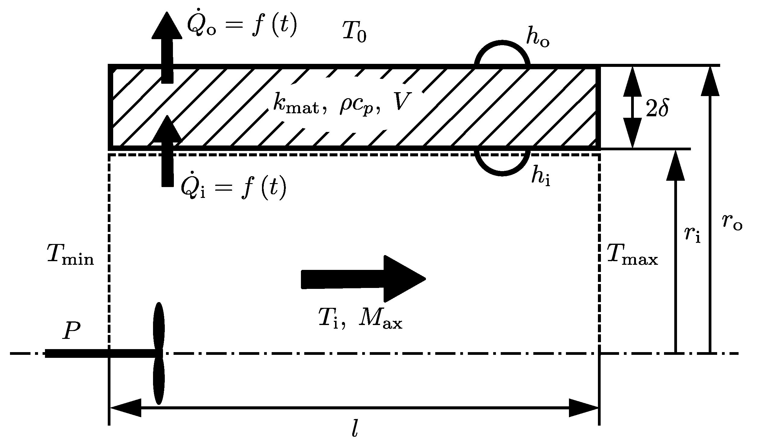
As described in Reference [18], a generalized flow-through system with input or output of shaft power P is used as a base substitute system for a turbomachine. It is characterized by the dimensional parameters shown in Figure 1 and Table 1. The inner heat flow ${\dot{Q}}_{\mathrm{i}}\left(t\right)$ and the outer heat flow ${\dot{Q}}_{\mathrm{o}}\left(t\right)$ differ in a time-dependent way in the present case of transient heat transfer. As shown in Equation (1), they are related by the rate of change in internal heat energy of the pipe structure,

$${\dot{Q}}_{\mathrm{i}}-{\dot{Q}}_{\mathrm{o}}=\rho c_p\frac{\partial T_{\mathrm{mat}}}{\partial t}.$$

(1)

Figure 1. Model of generalized turbomachine.

Table 1. Dimensional matrix used to derive the non-dimensional heat flow.

	${\dot{\mathit{Q}}}_{\mathbf{i}}$	${\mathit{T}}_{\mathbf{min}}-{\mathit{T}}_0$	${\mathit{T}}_{\mathbf{max}}-{\mathit{T}}_0$	$\mathit{\delta }$	${\mathit{A}}_{\mathbf{i}}$	${\mathit{A}}_{\mathbf{o}}$	${\mathit{h}}_{\mathbf{i}}$	${\mathit{h}}_{\mathbf{o}}$	${\mathit{k}}_{\mathbf{mat}}$	$\mathit{\rho }{\mathit{c}}_{\mathit{p}}$	V	t
L	2	0	0	1	2	2	0	0	1	−1	3	0
T	−3	0	0	0	0	0	−3	−3	−3	−2	0	1
M	1	0	0	0	0	0	1	1	1	1	0	0
Θ	0	1	1	0	0	0	−1	−1	−1	−1	0	0

The thermal properties of the substitute system are characterized by the inner and outer heat transfer coefficients $h_{\mathrm{i}}$ and $h_{\mathrm{o}}$, the thermal conductivity of the material $k_{\mathrm{mat}}$, the volumetric heat capacity $\rho c_p$, and the volume of the structure V. The input or output of shaft power is reflected by differing values of $T_{\min }$ and $T_{\max }$. As in Reference [16], the inner heat flow ${\dot{Q}}_{\mathrm{i}}\left(t\right)$ is divided into a steady state and a transient component,

$${\dot{Q}}_{\mathrm{i}}\left(t\right)={\dot{Q}}_{\mathrm{i},\mathrm{total}}\left(t\right)-{\dot{Q}}_{\mathrm{i}}\left(t\to \infty \right).$$

(2)

Consequently, the transient component of the inner heat flow can be expressed as a function of the dimensional parameters as:

$${\dot{Q}}_{\mathrm{i}}=f\left(t,T_{\min },T_{\max },T_0,\delta ,A_{\mathrm{i}},A_{\mathrm{o}},h_{\mathrm{i}},h_{\mathrm{o}},k_{\mathrm{mat}},\rho c_p,V\right).$$

(3)

In Equation (3), the surface areas $A_{\mathrm{i}}$ and $A_{\mathrm{o}}$ are directly related to $r_{\mathrm{i}}$ and $r_{\mathrm{o}}$, respectively, as well as the length $l$. The characteristic thickness $\delta$ of an arbitrary structure is the ratio of its volume to its surface area relevant to heat transfer [19].

Using the dimensional matrix shown in Table 1, the non-dimensional inner heat flow becomes a function of the non-dimensional parameters defined in Equations (4)–(8).

$$\begin{array}{cc}\hfill \frac{{\dot{Q}}_{\mathrm{i}}}{\left(T_{\max }-T_0\right)l_{\mathrm{ref}}{k}_{\mathrm{mat}}}& =f\left(\mathit{Fo},{\mathit{Bi}}_{\mathrm{i}},{\mathit{Bi}}_{\mathrm{o}},{\vartheta }_{\mathrm{char}},\frac{A_{\mathrm{o}}}{A_{\mathrm{i}}},\frac{A_{\mathrm{i}}}{{\delta }^2},\frac{V}{{\delta }^3}\right),\hfill \end{array}$$

(4)

$$\begin{array}{cc}\hfill \mathit{Fo}& =\frac{k_{\mathrm{mat}}t}{\rho c_p{\delta }^2},\hfill \end{array}$$

(5)

$$\begin{array}{cc}\hfill {\mathit{Bi}}_{\mathrm{i}}& =\frac{h_{\mathrm{i}}\delta }{k_{\mathrm{mat}}},\hfill \end{array}$$

(6)

$$\begin{array}{cc}\hfill {\mathit{Bi}}_{\mathrm{o}}& =\frac{h_{\mathrm{o}}\delta }{k_{\mathrm{mat}}},\hfill \end{array}$$

(7)

$$\begin{array}{cc}\hfill {\vartheta }_{\mathrm{char}}& =\frac{T_{\min }-T_0}{T_{\max }-T_0}.\hfill \end{array}$$

(8)

The non-dimensional temperature difference ratio ${\vartheta }_{\mathrm{char}}$ represents the operating point of the machine [18]. Since the Biot numbers can be expressed using the engine’s mass flow [16,18] and surface temperatures [18], they depend on the engine’s operating point, too. Hence, ${\vartheta }_{\mathrm{char}},{\mathit{Bi}}_{\mathrm{i}},{\mathit{Bi}}_{\mathrm{o}}$ are time-dependent parameters. The parameters $\frac{A_{\mathrm{o}}}{A_{\mathrm{i}}},\frac{A_{\mathrm{i}}}{{\delta }^2},\frac{V}{{\delta }^3}$ describe the geometry. The reference length $l_{\mathrm{ref}}$ is defined as

$$l_{\mathrm{ref}}=\frac{A_{\mathrm{i}}}{\delta }.$$

(9)

The basic form of the resulting non-dimensional transient heat transfer maps is derived assuming a straight pipe as a simple structural element.

3. Simulation

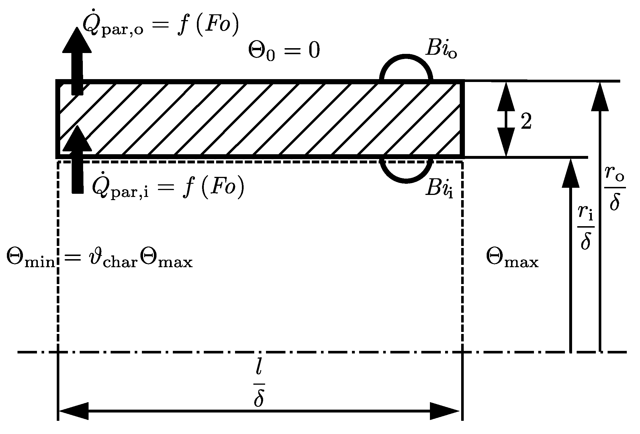
A two-dimensional finite element model is set up to derive the non-dimensional transient heat transfer maps based on the parameters shown in Figure 2. Assuming rotational symmetry, the simulation is carried out using MATLAB’s partial differential equation toolbox. For the simulation, a triangular mesh was generated. It consists of 25 470 elements with six nodes per element. The nodes are located at the corners and edge midpoints. To generate the mesh, the growth rate was set to 1.5, the target minimum element size to 0.05, and the target maximum element size to 0.1.

Figure 2. Non-dimensional parameters used for FEM simulation of the diabatic pipe flow.

The non-dimensional flow temperature $\mathrm{\Theta }$ describes the temperature of the fluid flow at a given position within the pipe. It is formed using the ambient temperature $T_0$ and the initial maximum temperature $T_{\max ,\mathrm{ini}}$ as references:

$$\mathrm{\Theta }=\frac{T-T_0}{T_{\max ,\mathrm{ini}}-T_0}.$$

(10)

To verify the simulation setup, the results were compared to the heat transfer of a lumped capacitance, for which an analytical solution exists [19]. To do so, uniform temperature around the system was assumed, and a unit-step was simulated by setting

$$\begin{array}{cc}\hfill t=0:& {\mathrm{\Theta }}_{\min }={\mathrm{\Theta }}_{\max }={\mathrm{\Theta }}_0=0,\hfill \end{array}$$

(11)

$$\begin{array}{cc}\hfill t>0:& {\mathrm{\Theta }}_{\min }={\mathrm{\Theta }}_{\max }={\mathrm{\Theta }}_0=1.\hfill \end{array}$$

(12)

Furthermore, the Biot numbers ${\mathit{Bi}}_{\mathrm{i}}$ and ${\mathit{Bi}}_{\mathrm{o}}$ are set equally. The material properties and the non-dimensionals describing the geometry are kept constant. The Root Mean Squared Percentage Error of the verification was smaller than 0.1% This indicates a good match between the predicted heat transfer of the FEM simulation and the lumped capacitance.

After verifying the model, it is now used to derive the non-dimensional transient heat transfer maps. The material properties and the non-dimensionals describing the geometry are kept constant for the following steps. The non-dimensional flow temperature is assumed to vary inside the system linearly from ${\mathrm{\Theta }}_{\min }$ to ${\mathrm{\Theta }}_{\max }$. The non-dimensional temperature difference ${\vartheta }_{\mathrm{char}}$ is the ratio of the non-dimensional flow temperatures ${\mathrm{\Theta }}_{\min }$ to ${\mathrm{\Theta }}_{\max }$,

$${\vartheta }_{\mathrm{char}}=\frac{{\mathrm{\Theta }}_{\min }}{{\mathrm{\Theta }}_{\max }}=\frac{\frac{T_{\min }-T_0}{T_{\max ,\mathrm{ini}}-T_0}}{\frac{T_{\max }-T_0}{T_{\max ,\mathrm{ini}}-T_0}}.$$

(13)

The transient response of the system is identified by simulating step changes in ${\mathrm{\Theta }}_{\max }$ of different sizes ${\mathrm{\Theta }}_{\mathrm{step}}$:

$$\begin{array}{cc}\hfill t=0:& {\mathrm{\Theta }}_{\max }=1,\hfill \end{array}$$

(14)

$$\begin{array}{cc}\hfill t>0:& {\mathrm{\Theta }}_{\max }=1+{\mathrm{\Theta }}_{\mathrm{step}}=1+\frac{T_{\max }-T_{\max ,\mathrm{ini}}}{T_{\max ,\mathrm{ini}}-T_0}.\hfill \end{array}$$

(15)

This approach maps step changes in thermal load of different sizes. The temperature ${\mathrm{\Theta }}_{\min }$ follows according to Equation (13). With constant ambient temperature $T_0$, the outside temperature ratio stays constant at ${\mathrm{\Theta }}_0=0$.

${\mathit{Bi}}_{\mathrm{i}},{\mathit{Bi}}_{\mathrm{o}}$, and ${\vartheta }_{\mathrm{char}}$ are kept constant during the step changes. They are varied for the individual step changes such that the operating ranges of the compressor and the turbine of the investigated engine are well covered by the simulation. Consequently, the Biot numbers are chosen to be distributed evenly in the logarithm to base 10 (lg) space,

$$\begin{array}{c}-3.8\le lg\left({\mathit{Bi}}_{\mathrm{i}}\right)\le -0.8,\end{array}$$

(16)

$$\begin{array}{c}-5.4\le lg\left({\mathit{Bi}}_{\mathrm{o}}\right)\le -2.4.\end{array}$$

(17)

${\vartheta }_{\mathrm{char}}$ is selected from an interval from −0.05 to 0.15 and from 0.65 to 1 to reflect possible values for the investigated compressor and turbine, respectively.

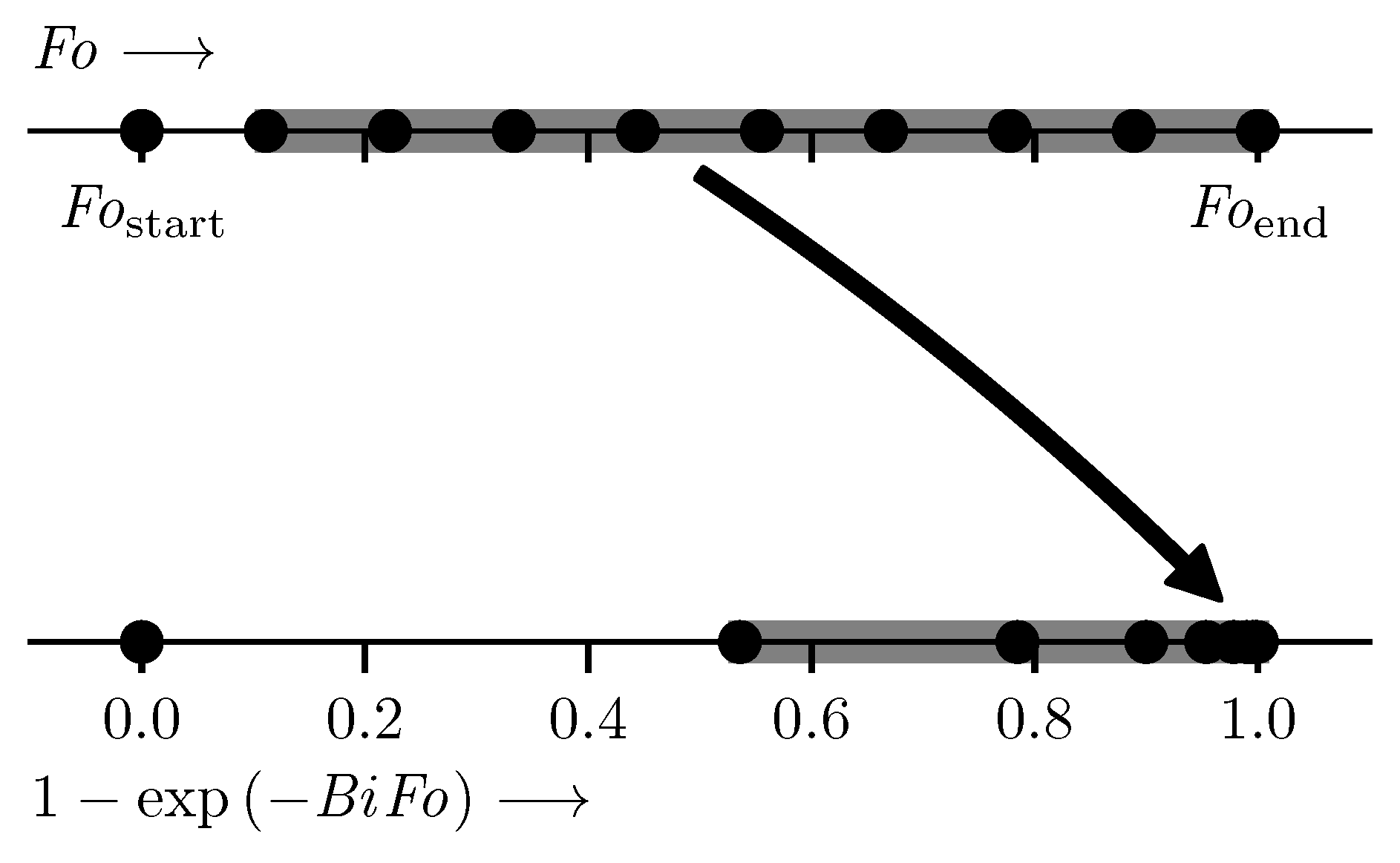
The data is sampled for each simulation at different Fourier numbers. The rationale behind the distribution of the sample points is based on the transient response of a lumped capacitance, which can be expressed as [19]:

$$\dot{Q}=f\left(exp\left(-\mathit{BiFo}\right)\right).$$

(18)

At constant Biot number $\mathit{Bi}$, the heat flow $\dot{Q}$ reduces with increasing Fourier number $\mathit{Fo}$. As indicated in Figure 3, sampling the transient response at constant intervals of Fourier number $\mathit{Fo}$ would cluster the sampling points at low heat flows. Consequently, the part of the step response featuring significant change in heat flow rates would be underrepresented in the data. Hence, the data points were sampled linearly with respect to $1-exp\left(-\mathit{BiFo}\right)$.

Figure 3. Effect of linearly spacing $\mathit{Fo}$.

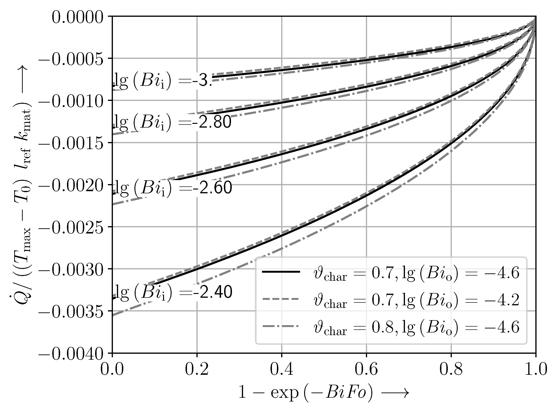
The non-dimensional transient heat transfer map derived from FEM simulation for a given step change of ${\mathrm{\Theta }}_{\mathrm{step}}=1.0$ is shown in Figure 4 for sets of parameters ${\mathit{Bi}}_{\mathrm{i}}$, ${\mathit{Bi}}_{\mathrm{o}}$, and ${\vartheta }_{\mathrm{char}}$. It becomes obvious that the variation of the non-dimensional heat transfer map as a function of these parameters is relevant.

Figure 4. Non-dimensional transient heat transfer map for a given step change of ${\mathrm{\Theta }}_{\mathrm{step}}=1$.

The shapes of the non-dimensional heat transfer maps resulting from different step responses are shown in Figure 5a. A change of sign of the step change results in a different shape of the maps. As shown in Figure 5b, these lines collapse with variation due to the parameters ${\mathit{Bi}}_{\mathrm{i}}$, ${\mathit{Bi}}_{\mathrm{o}}$, and ${\vartheta }_{\mathrm{char}}$ remaining, if the non-dimensional heat flow is referred to the size of the non-dimensional temperature step. This normalizing step leads to

$$\frac{{\dot{Q}}_{\mathrm{i}}}{{\mathrm{\Theta }}_{\mathrm{step}}\left(T_{\max }-T_0\right)l_{\mathrm{ref}}{k}_{\mathrm{mat}}}=\frac{{\dot{Q}}_{\mathrm{i}}}{\left(T_{\max }-T_{\max ,\mathrm{ini}}\right)l_{\mathrm{ref}}{k}_{\mathrm{mat}}},$$

(19)

which is in accordance with the approach shown in References [16,20]. Furthermore, the heat transfer map shown in Figure 5b is insensitive to variation in geometry.

Figure 5. (a) Non-dimensional heat transfer map for varying step changes; (b) non-dimensional heat transfer map after referring heat flow to step size.

The maps obtained from the FEM simulation are used to train a neural network. This is the basis for transient heat transfer modeling of turbomachines using transfer learning.

4. Encoding the Non-Dimensional Maps Using Neural Networks

In a first step a suitable type of neural network is selected. With the thermal transients representing a time series possible choices for the networks are:

• Feedforward Networks, e.g., Multilayer Perceptron (MLP);
• Recurrent Neural Networks:

  -

  Shallow Networks, e.g., Non-linear Autoregressive Network with Exogenous Inputs (NARX);

  -

  Deep Networks, e.g., Long Short-Term Memory (LSTM).

Both shallow and deep recurrent neural networks directly model the time dependency in their architecture. However, transfer learning using a recurrent neural network is challenging. Using a feedforward neural network, such as a Multilayer Perceptron, follows the principle of directly modeling the non-dimensional transient heat transfer maps. They cover the step responses of the non-dimensional heat flow

$${\dot{Q}}_{\mathrm{par}}=\frac{{\dot{Q}}_{\mathrm{i}}}{{\mathrm{\Theta }}_{\mathrm{step}}\left(T_{\max }-T_0\right)l_{\mathrm{ref}}{k}_{\mathrm{mat}}}$$

(20)

at constant ${\mathit{Bi}}_{\mathrm{i}}$, ${\mathit{Bi}}_{\mathrm{o}}$, and ${\vartheta }_{\mathrm{char}}$ and varying Fourier numbers $\mathit{Fo}$. Since a Multilayer Perceptron can approximate any function [21], the transient heat transfer map of the pipe can be modeled by an MLP. Therefore, an MLP was chosen with $\mathit{Fo}$, $lg\left({\mathit{Bi}}_{\mathrm{i}}\right)$, $lg\left({\mathit{Bi}}_{\mathrm{o}}\right)$, and ${\vartheta }_{\mathrm{char}}$ as features, and ${\dot{Q}}_{\mathrm{par}}$ as target, for the following steps.

A total of 4096 different step responses were simulated. Sixty percent of the data was used for training, and 20% for test and validation, respectively.

Random sampling of training and test data sets generally guarantees that the trained network can interpolate points on the maps. However, if the trained network is able to predict a whole step response, which it has previously not seen, it can be assumed that the network captures the underlying physics.

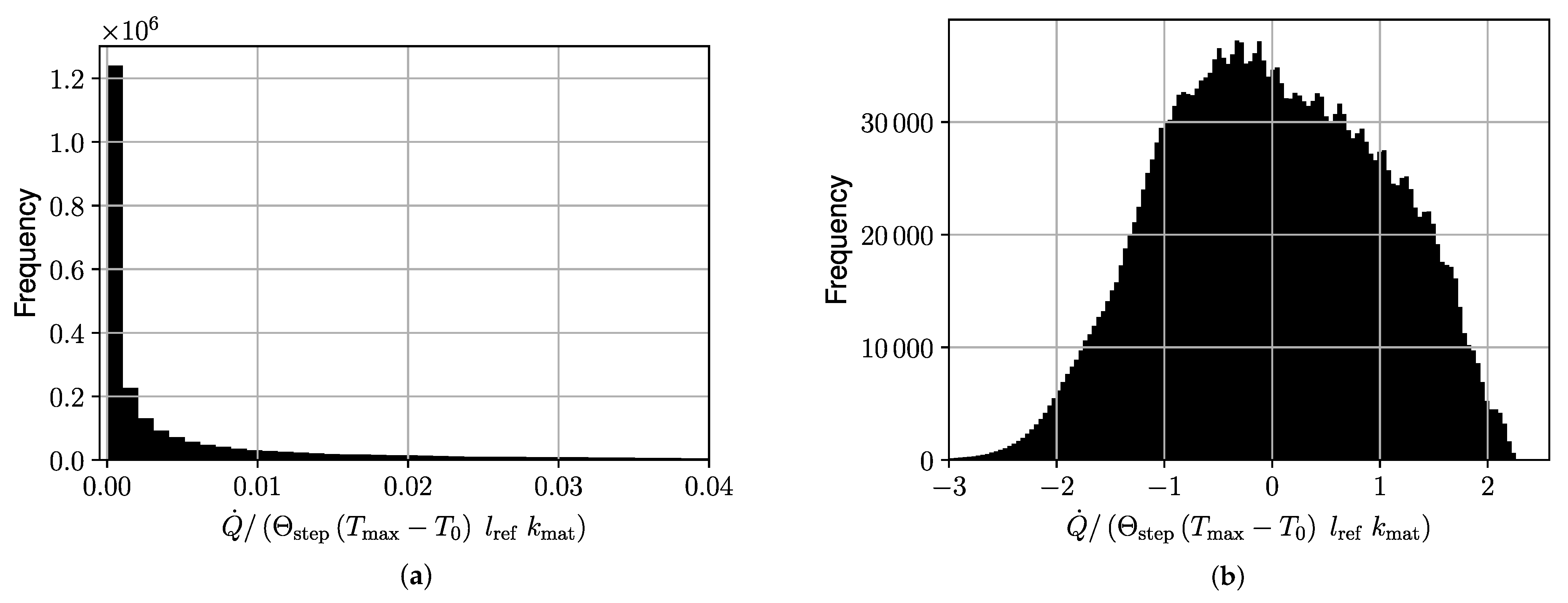
Without an additional transformation, the data is clustered towards small values of ${\dot{Q}}_{\mathrm{par}}$, as can be seen in Figure 6a. To approximate a normal distribution of the data, the Box-Cox transform, as implemented in SciPy [22], is used on the training data. It is defined as

$${\dot{Q}}_{\mathrm{par},\mathrm{trans}}=\left\{\begin{array}{cc}\frac{{\dot{Q}}_{\mathrm{par}}-1}{\lambda }\hfill & \mathrm{if} \lambda \ne 0,\hfill \\ log\left({\dot{Q}}_{\mathrm{par}}\right)\hfill & \mathrm{if} \lambda =0.\hfill \end{array}\right.$$

(21)

Figure 6. Histogram of targets in training set (a) before scaling and (b) after scaling.

The value of the parameter $\lambda$ was estimated, using maximum likelihood estimation, to be $\lambda =0.053$. Additionally, the targets are standardized to zero mean and unit variance to facilitate better training. The histogram of the transformed ${\dot{Q}}_{\mathrm{par}}$ is shown in Figure 6b. The features $\mathit{Fo}$, $lg\left({\mathit{Bi}}_{\mathrm{i}}\right)$, $lg\left({\mathit{Bi}}_{\mathrm{o}}\right)$, and ${\vartheta }_{\mathrm{char}}$ are all normalized to fall in the interval $\left[0,1\right]$.

A grid search was carried out to obtain a good architecture. For this purpose the number of hidden layers was varied from one to three. The number of neurons per layer was varied, too. For all architectures, the number of neurons decreases the deeper the layer, resulting in a pyramid-shaped architecture. This is done to compress the information from hidden layer to hidden layer to predict ${\dot{Q}}_{\mathrm{par}}$. All hidden layers feature rectified linear units as activation functions.

Training was performed using PyTorch [23] and fastai v1 [24]. The 1-cycle policy [25,26] was applied to training, where the learning rate is first increased and then decreased during training, while the opposite is done for momentum. The maximum value for the learning rate was set using a learning rate finder as described in Reference [24]. Weight decay was chosen to achieve the highest learning rates [26]. A total number of 120 epochs was sufficient to achieve good results.

The performance of the different architectures was evaluated using the Root Mean Squared Error (RMSE) on the validation data. Table 2 shows results of investigated architectures.

Table 2. Root Mean Squared Error (RMSE) of different architectures. The architecture with the lowest RMSE is marked in bold font.

Architecture No.	Number of Hidden Layers	Number of Neurons in the Hidden Layers	Number of Parameters	RMSE
1	1	250	1501	0.0527
2	1	450	2701	0.0627
3	2	300, 100	31 701	0.0133
4	2	250, 200	51 651	0.0112
5	2	400, 200	82 401	0.0143
6	2	500, 250	128 001	0.0169
7	3	50, 25, 10	1796	0.0212
8	3	100, 50, 25	6851	0.0524
9	3	150, 100, 50	20 951	0.0136
10	3	200, 100, 50	26 201	0.0104
11	3	250, 100, 10	27 371	0.0117
12	3	200, 150, 50	38 751	0.0126
13	3	250, 150, 10	40 421	0.0120
14	3	250, 150, 50	46 501	0.0095
15	3	200, 200, 50	51 301	0.0106
16	3	250, 200, 50	61 551	0.0115
17	3	300, 200, 100	81 901	0.0124
18	3	500, 200, 100	122 901	0.0120

Since all layers in the network are fully connected, the number of trainable parameters can be calculated using the number of inputs $n_{\mathrm{in}}$ and the number of outputs $n_{\mathrm{out}}$ of each layer by

$$n_{\mathrm{param}}=\sum _{j=1}^k\left(n_{\mathrm{in},\mathrm{j}}·n_{\mathrm{out},\mathrm{j}}\right)+\sum _{j=1}^k{n}_{\mathrm{out},\mathrm{j}}.$$

(22)

In Equation (22), k is the number of layers in the architecture, which includes the output layer. The first sum reflects the trainable weights, and the second sum reflects the trainable bias. The same total number of neurons in the hidden layers can result in a different number of trainable parameters. This becomes obvious by comparing, e.g., architecture No. 2 with architecture No. 14, shown in Table 2. 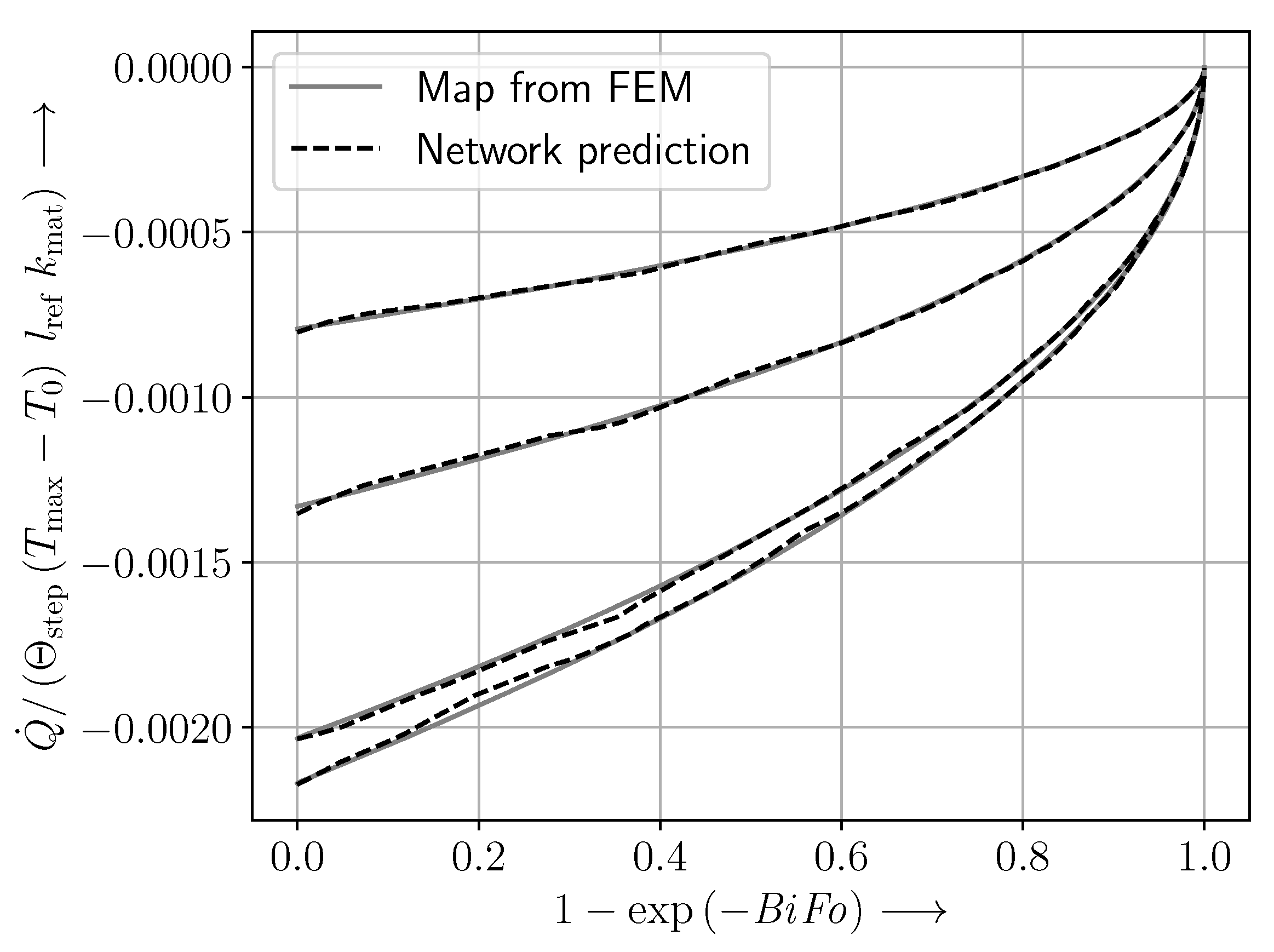For three-layer architectures the RMSE of the validation data shown in Table 2 falls to a minimum and then increases with increasing number of parameters. This indicates that there is an optimum for the number of neurons per layer. Furthermore, three hidden layers perform better than two hidden layers with a similar amount of trainable parameters. Overall, good performance was achieved using a three-layer MLP with 250, 150, and 50 neurons in the first, second, and third hidden layer, respectively. The quality of the achieved prediction is documented in Figure 7, where four step responses that are all part of the test set are shown. As can be seen, the network approximates the results from the FEM simulation well.

Figure 7. Quality of transient heat transfer map prediction using Multilayer Perceptron.

5. Measured Data Used for Transfer Learning

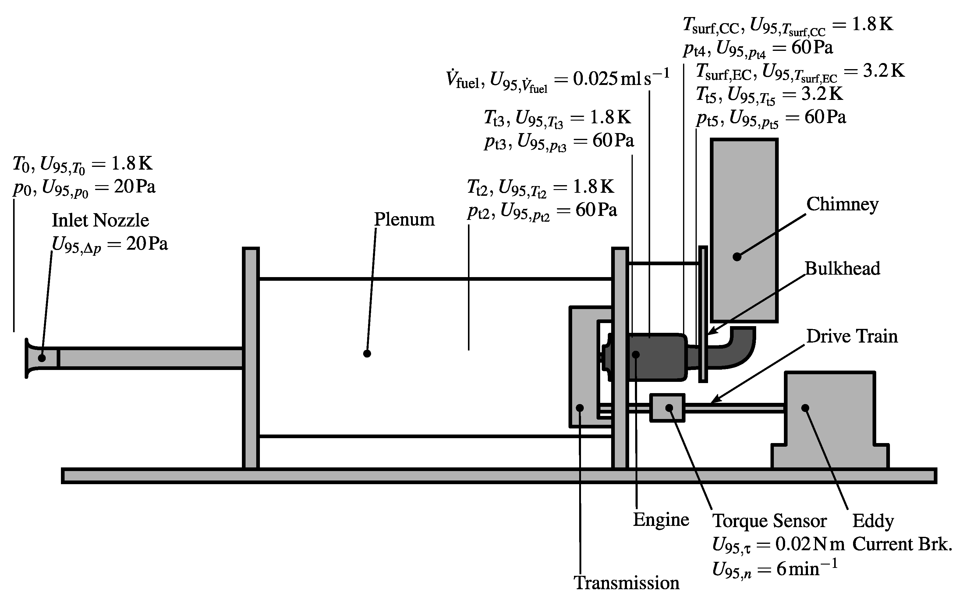
The test rig as described in Reference [18] is used to provide measured data for transfer learning, as well as testing and validation, of the model. It comprises the engine, whose transient thermal response will be modeled using transfer learning. Temperatures are measured using Typ K thermocouples, while Netscanner pressure sensor were used to measure the gas path pressures. The engine’s mass flow $\dot{m}$ is measured using an inlet nozzle. Flow around the engines is blocked by the bulkhead. This ensures that only natural convection and thermal radiation have to be considered when calculating ${\mathit{Bi}}_{\mathrm{o}}$. The transmission system features a dedicated torque sensor. The experimental setup, the instrumentation, and the systematic parts of the sensor uncertainties are shown in Figure 8.

Figure 8. Experimental setup, instrumentation, and systematic part of sensor uncertainties.

To use the measurements from this rig for transfer learning, a total of 20 different maneuvers were carried out. The maneuvers were designed to cover the operating range of the engine. As mentioned earlier, the Biot numbers are a function of the engine’s mass flow and the temperatures. Additionally, ${\vartheta }_{\mathrm{char}}$ is directly related to the temperatures present in the engine (see Equation (8)). Hence, varying acceleration and deceleration maneuvers were carried out along the operating line with low shaft power output $P_{\mathrm{Brk}}$. The minimum rotational speed was at 60 000 min${}^{-1}$, while the maximum rotational speed was at 94 000 min${}^{-1}$. This varies the engine’s mass flow and, also, moderately, the temperatures. For this particular engine, the temperatures vary significantly when the engine is loaded. Therefore, the engine was loaded or unloaded transiently at maximum rotational speed during some maneuvers by varying the shaft power output $P_{\mathrm{Brk}}$ using the test rig’s eddy current brake. The power level at the end of the loading maneuvers was varied, as well as the the time to load or unload the engine. All of the measured maneuvers resemble step responses. Since the maps obtained from the FEM simulation represent the unit step response of a pipe, data obtained from these maneuvers is well suited for transfer learning.

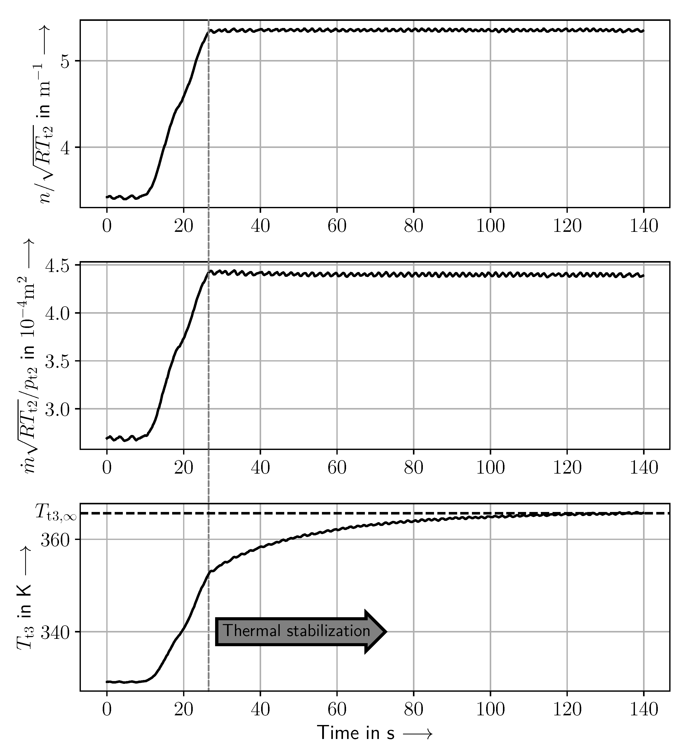
The time series of parameters measured during a typical acceleration maneuver is shown in Figure 9. The acceleration is started at $t=9$ s. At $t=26.5$ s, the compressor has reached steady state non-dimensional speed $n/\sqrt{R{T}_{t2}}$ and mass flow parameter $\dot{m}\sqrt{R{T}_{t2}}/p_{t2}$. Until $t=140$ s, the compressor exit temperature $T_{t3}$ keeps creeping towards its steady state level $T_{t3,\infty }$. This indicates continuing heat transfer, since tip clearance effects are assumed to be negligible for this type of engines [27].

Figure 9. Compressor data for a typical acceleration maneuver.

At a given point in time t, the heat flow from the fluid to the compressor structure is computed using

$${\dot{Q}}_{(}t)=\dot{m}\left(t\right)\left(h_{t3}\left(t\right)-h_{t3}\left(t\to \infty \right)\right).$$

(23)

The total enthalpies in Equation (23) are calculated using the respective total temperatures and a fluid model typical for today’s gas turbine engine performance programs. The temperatures used to calculate $h_t$ were measured directly. The temperature readings are corrected to account for the thermal inertia of the thermocouples [28]. The actual temperature $T_{\mathrm{actual}}$ is related to the reading $T_{\mathrm{reading}}$ by

$$T_{\mathrm{actual}}=t_{63.2\%}\frac{d{T}_{\mathrm{reading}}}{dt}+T_{\mathrm{reading}}.$$

(24)

The time constant $t_{63.2\%}$ is calculated according to Reference [28] using the values of the time constants given in the data sheet of the thermocouples. Only the part of the maneuvers during thermal stabilization, as indicated in Figure 9, is used to calculate the heat flow.

The characteristic non-dimensional temperature difference ${\vartheta }_{\mathrm{char}}$ directly results from the measurements. According to Equation (13), it is zero for the investigated compressor, since the entry temperature into the compressor $T_{t,\min }\approx T_0$.

Calculation of the Biot numbers follows the same principles as described in Reference [18]. For ${\mathit{Bi}}_{\mathrm{o}}$ of the compressor, only free convection is considered, due to the special setting at the test bed [18].

The two parts of the centrifugal compressor’s casing feature different radii. The casing is, therefore, modeled as an equivalent pipe (see Figure 10). This approach ensures consistency with the assumptions underlying the non-dimensional transient heat transfer maps. This equivalent radius $r_{\mathrm{equ}}$ is calculated by requiring that the heat flow due to free convection stays the same for the equivalent pipe,

$${\dot{Q}}_{\mathrm{equ},\mathrm{free}}={\dot{Q}}_{\mathrm{in},\mathrm{free}}+{\dot{Q}}_{\mathrm{out},\mathrm{free}}.$$

(25)

Assuming a constant temperature difference and constant $k_{\mathrm{mat}}$, Equation (25) can be written as

$$\frac{{\mathit{Nu}}_{\mathrm{equ}}{A}_{\mathrm{equ}}}{l_{\mathrm{equ}}}=\frac{{\mathit{Nu}}_{\mathrm{in}}{A}_1}{l_{\mathrm{in}}}+\frac{{\mathit{Nu}}_{\mathrm{out}}{A}_{\mathrm{out}}}{l_{\mathrm{out}}}.$$

(26)

Finally, Equation (27) is derived using the Nusselt correlation for an isothermal horizontal cylinder [29],

$$r_{\mathrm{equ}}^{-0.25}=\frac{r_{\mathrm{in}}^{0.75}{l}_{\mathrm{in}}+r_{\mathrm{out}}^{0.75}{l}_{\mathrm{out}}}{r_{\mathrm{in}}{l}_{\mathrm{in}}+r_{\mathrm{out}}{l}_{\mathrm{out}}}.$$

(27)

Figure 10. Modeling the compressor casing as an equivalent pipe.

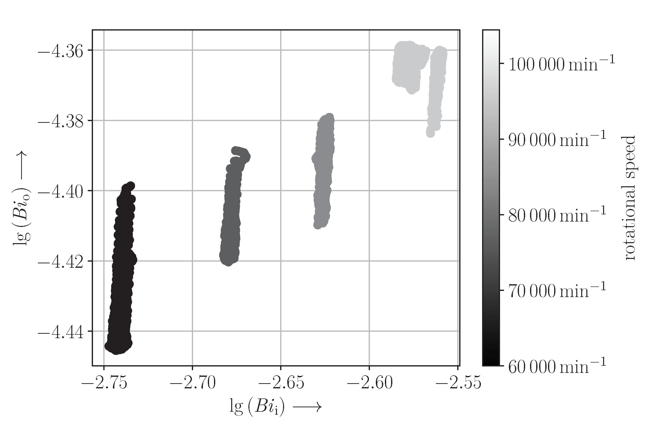
The inner and outer Biot numbers both vary in a limited range for the example radial compressor (see Figure 11).

Figure 11. Scatter plot of experimentally-identified Biot numbers in the compressor.

The Biot numbers of the turbine are identified as described in Reference [18]. The heat flow $\dot{Q}$ is derived indirectly since the combustor exit temperature $T_{t4}$ cannot be measured with adequate accuracy. $T_{t4}\left(t\right)$ is synthesized as a function of time t from the combustor heat balance reflecting the compressor heat transfer,

$$\begin{array}{c}\hfill \dot{m}\left(t\right)h_{t3}\left(t\right)+{\dot{m}}_{fuel}\left(t\right)LHV{\eta }_{CC}={\dot{m}}_4\left(t\right)h_{t4}\left(t\right),\end{array}$$

(28)

$$\begin{array}{c}\hfill {\dot{m}}_4\left(t\right)=\dot{m}\left(t\right)+{\dot{m}}_{fuel}\left(t\right).\end{array}$$

(29)

It becomes obvious that $T_{t4}$ only depends on the transient performance of the compressor and, hence, is not influenced by the thermal transient of the turbine. Consequently, the heat flow of the turbine can be calculated using

$$\begin{array}{c}\hfill {\dot{m}}_4{\left(h_{t4}-h_{t5}\right)}_{\mathrm{dia}\mathrm{Comp}}={\dot{m}}_4{\left(h_{t4}-h_{t5}\right)}_{\mathrm{dia}}+\dot{Q},\end{array}$$

(30)

$$\begin{array}{c}\hfill \dot{Q}={\dot{m}}_4\left(h_{t5,\mathrm{dia}.\mathrm{Comp}.}-h_{t5,\mathrm{measured}}\right).\end{array}$$

(31)

The temperature measurements used to calculate $h_{t5,\mathrm{measured}}$ are again corrected to account for the thermal inertia (see Equation (24)). Both $T_{t5,\mathrm{dia}.\mathrm{Comp}.}$ and $T_{t5,\mathrm{measured}}$ were filtered to reduce the high amount of noise. Additionally, $T_{t5,\mathrm{measured}}$ was shifted, so that

$$T_{t5,\mathrm{dia}.\mathrm{Comp}.}\left(t\to \infty \right)=T_{t5,\mathrm{measured}}\left(t\to \infty \right).$$

(32)

This is done to account for deviations in the stationary performance model, thereby ensuring that ${\dot{Q}}_{\left(t\to \infty \right)}=0$. The experimentally-identified data is now used to transfer the non-dimensional heat transfer maps encoded by the MLP from the pipe to the engine.

6. Transfer Learning

First, a constant scaling factor representing the circumference of the equivalent pipe is introduced at the end of the network to consider three-dimensional effects not covered by the simulation. This enabled easier and faster training.

In general, transfer learning is done in three steps. In the first step, additional hidden layers are added to the end of the network. For both the compressor and the turbine, one additional layer consisting of 25 neurons and rectified linear unit activations was sufficient. In the second step, only the additional hidden layers are trained using the experimentally-identified data. In the third step, the rest of the network is unfrozen, and all the layers are trained with a low learning rate. This third step is often referred to as fine tuning.

Since there are only 20 maneuvers, 16 were used for training, while 4 were used as test set. It was made sure that maneuvers from similar operating conditions were grouped together. This prevents data leaking from the training set into the test set and ensures that the network properly generalizes.

Following Equations (28)–(31), the thermal transient of the compressor is required to derive the thermal transient of the turbine. Hence, results achieved for the compressor are discussed first. The measurements did not show large variation in the non-dimensional parameters, as shown for the Biot numbers in Figure 11.

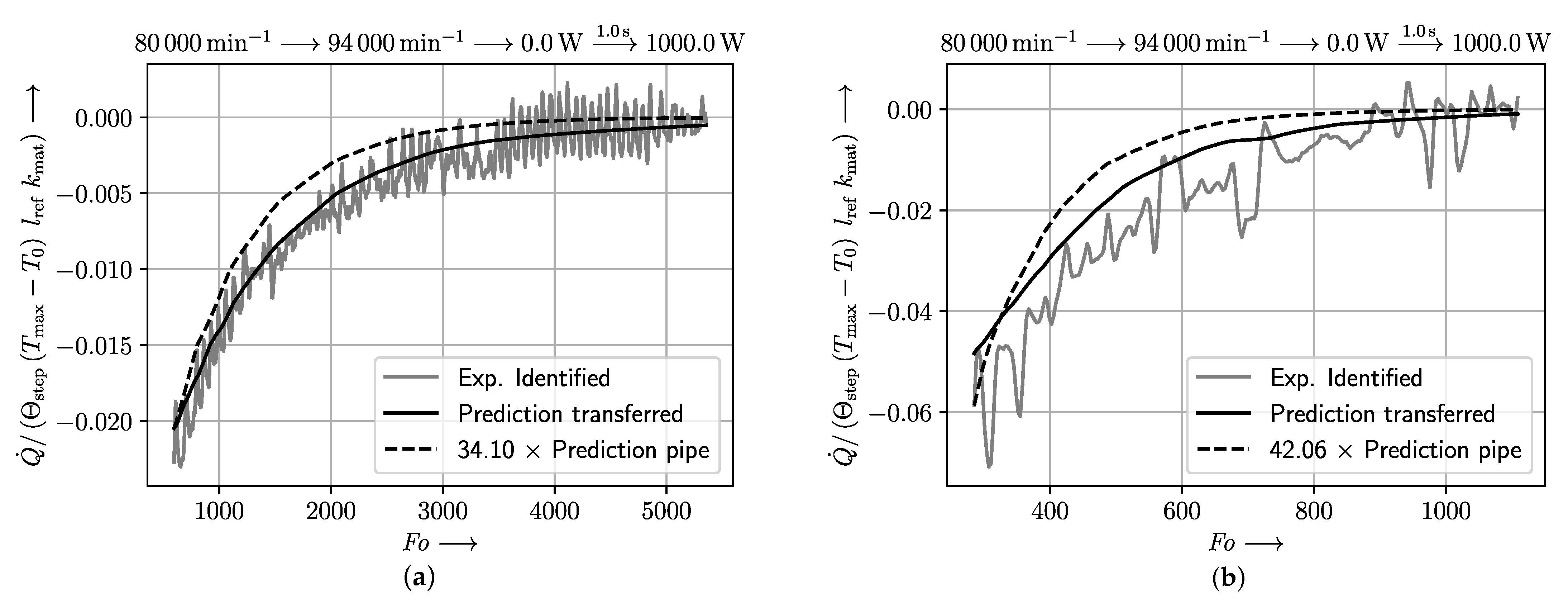
One experimentally-identified step response of the compressor’s non-dimensional transient heat flow is shown in Figure 12a. It features significant noise. This is attributed to the correction of the temperature readings, as described in Equation (24). In Figure 12a, the prediction of the original network, that represents the thermal transient of a pipe, is compared to the prediction of the transferred neural network. The prediction of the original network needs to be scaled to meet the range of the measured data. The scaling factor is displayed in the legend of Figure 12. However, the thermal transient of the compressor is slower due to the large thermal mass of the compressor’s impeller and its bladed diffuser. Hence, it is the step of transfer learning which improves the prediction by matching not only the measured range but also the time constant. This is visible by comparing the rise times of the two different predictions shown in Figure 12a.

Figure 12. Comparison of experimentally-identified non-dimensional transient heat flow to scaled non-transferred network, that encodes the thermal transient of a pipe and to transfer-learned network for (a) compressor and (b) turbine, experimentally-identified step response filtered.

The thermal transient of the turbine is identified based on these results. Despite filtering the temperatures, the scatter of the experimentally-identified step response of the turbine shown in Figure 12b is still clearly visible. Again, the introduction of a constant scaling factor ensures the prediction using the thermal transient of a pipe meet the measured range. The time constant is better matched if transfer learning is applied.

7. Application to Gas Turbine Prediction

The neural networks representing the non-dimensional transient heat transfer maps of compressor and turbine were implemented into a state of the art gas turbine performance program to model the investigated shaft power engine. As shown in Equation (19), the transferred maps refer the heat flow to a jump in temperature. Therefore, the total heat flow of a component is modeled by superposing the heat flows resulting from their respective temperature jumps at the different time steps. 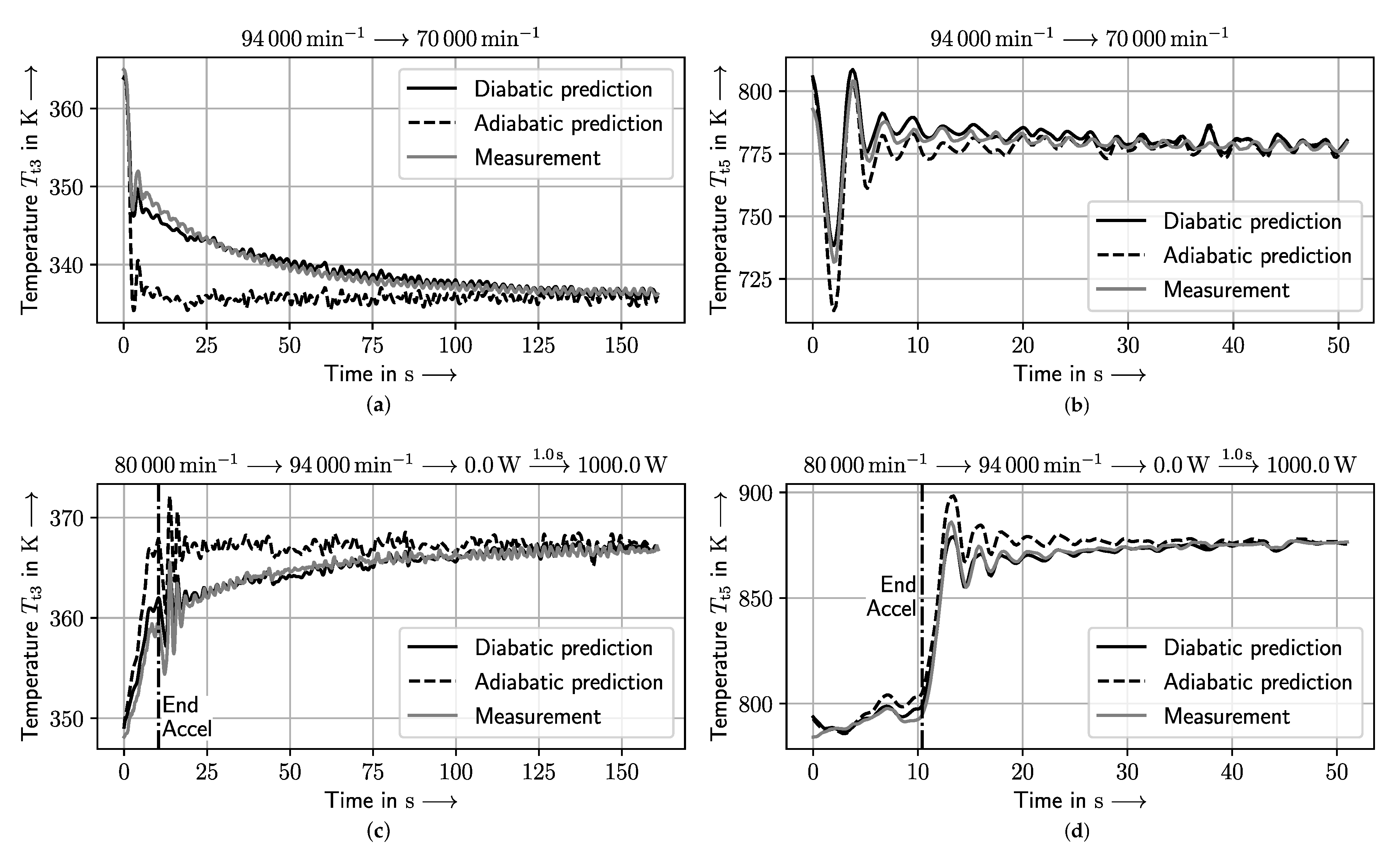This follows the same approach used in Reference [16]. The performance model is run to the measured fuel flow, which eliminates potential uncertainties in the modeling of the gas turbine control system. The changes in shaft power are measured on the testbed. They are an input to the performance model. The achieved quality of prediction is demonstrated for two exemplary maneuvers:

-

Deceleration from 94 000 min${}^{-1}$ to 70 000 min${}^{-1}$;

-

Acceleration from 80 000 min${}^{-1}$ to 94 000 min${}^{-1}$, followed by a change in shaft power of 1 $\mathrm{s}$ duration to a load of 1000 $\mathrm{W}$.

The comparison of the predicted and measured total temperature at compressor exit $T_{t3}$ indicates the quality of the diabatic compressor modeling achieved by the transferred maps. The comparison of the predicted and measured total temperatures at turbine exit $T_{t5}$ is used to indicate the quality of diabatic turbine modeling. It further embraces the quality of diabatic compressor modeling and the quality of the assumptions needed for the combustor energy balance documented in Equation (28).

The results obtained for both maneuvers are documented in Figure 13, where the measured total temperatures are compared to the diabatic and adiabatic prediction. Here, adiabatic prediction refers to the performance model without using the neural network to account for the engine’s thermal response. In Figure 13c,d, the end of the acceleration is marked by a vertical line. To analyze the quality of the transient model, the predictions are corrected for deviations in the stationary performance model, so that

$$T_{t,\mathrm{prediction}}\left(t\to \infty \right)=T_{t,\mathrm{measured}}\left(t\to \infty \right).$$

(33)

Figure 13. Comparison of measurement, adiabatic prediction (performance model without the neural network to model heat transfer), and diabatic prediction (same performance model with the neural network). Predictions are corrected for deviations in the stationary performance model; see Equation (33). (a) Compressor exit temperature, deceleration, (b) turbine exit temperature, deceleration, (c) compressor exit temperature, acceleration (accel), and loading, and (d) turbine exit temperature, acceleration (accel), and loading.

It becomes obvious that adiabatic modeling of the compressor does not lead to a time series of $T_{t3}$, which matches the time constant and the temperature level of the measurements. Diabatic compressor modeling using the non-dimensional transient heat transfer maps significantly improves the prediction of time constant and temperature level.

Consequently, the discussion regarding the turbine exit temperature $T_{t5}$ is based only on diabatic compressor modeling. The measured time series of turbine exit temperature $T_{t5}$ is matched well by the enhanced gas turbine model. The deviations visible can be explained with higher measurement uncertainty in $T_{t5}$ and more noise present in the signal. This makes transfer learning more difficult, which is also evident in Figure 12b.

Figure 13 shows that the thermal transient of the turbine is faster than the thermal transient of the compressor. This is in accordance with the larger thermal mass of the centrifugal compressor.

8. Generalization of the Method

Generally, the proposed method is directly usable for large gas turbine engines. It relies on typical measurement positions in such turbines. Different methods to derive the combustor exit temperature $T_{t4}$, such as combustor heat balance or turbine capacity method, are directly applicable.

However, the ranges for Biot number and ${\vartheta }_{\mathrm{char}}$ are quite different for larger engines [18]. This can be accounted for by expanding the ranges of the parameters in the two-dimensional FEM simulation. Additionally, tip clearance changes may play an important role in larger aero engines [9]. Hence, so-called cold stabilization maneuvers are not suited to support the required transfer learning. Hot reslam maneuvers featuring high heat flows are suggested for transfer learning. Different start and end conditions of the hot reslams should be chosen to increase the variability in the data. Furthermore, slam accelerations might be used, if the effects of heat transfer is significantly bigger than the effect of tip clearance changes.

The most time-consuming part of the proposed approach is the FEM simulation and the training of the original network encoding the results of the FEM. Transfer learning takes only a small amount of time. If the parameter range of the FEM simulation is chosen to be wide enough, the first two steps have to be carried out only once. The results of these steps could then be used to transfer the thermal behavior of an entire fleet.

Due to the dimensional analysis, this method is applicable to any system that can be be based on a system according to Figure 1 and Table 1. Additionally, the system and the dimensional analysis can be expanded to explicitly model further effects, such as cooling flows, by including the relevant parameters. The resulting non-dimensionals from the expanded dimensional analysis need to be included into the FEM simulation and used as features of the neural network used to encode the simulation results.

9. Conclusions and Outlook

Modeling transient turbomachinery heat transfer using non-dimensional heat transfer maps and neural networks is successfully demonstrated using a very small gas turbine as an example. Such a small gas turbine represents a worst case scenario, since the heat transfer within the components is superimposed by significant heat conduction between the components. Scaling of the non-dimensional transient heat transfer maps and transfer learning are required to match the engine thermal transients. The approach to use transfer learning has the advantage that only a limited amount of data is needed to obtain sufficient accuracy.

In a next step, the transferred networks can be used to regenerate the transient heat transfer maps. Those maps can then be directly implemented into the performance program as lookup tables. This should lead to very fast calculation times of the thermal transients. In addition, the results of the transfer learning and, therefore, the thermal transients can be interpreted by looking at the regenerated maps.