Abstract
A practical approach for deriving the absolute density field based on the background-oriented schlieren method in a high-speed flowfield was implemented. The flowfield of interest was a two-dimensional compressible flowfield created by two supersonic streams to simulate a linear aerospike nozzle operated under a supersonic in-flight condition. The linear aerospike nozzle had a two-dimensional cell nozzle with a design Mach number of 3.5, followed by a spike nozzle. The external flow simulating the in-flight condition was 2.0. The wall density distribution used as the wall boundary condition for Poisson’s equation to solve the density field was derived by a simplified isentropic assumption based on the measured wall pressure distribution, and its validity was evaluated by comparing with that predicted by numerical simulation. Unknown coefficients in Poisson’s equation were determined by comparing the wall density distribution with that predicted by the model. By comparing the derived density field based on the background-oriented schlieren method to that predicted by the model and numerical simulation, the absolute density field was derived within an error of 10% on the wall distribution. This practical approach using a simplified isentropic assumption based on measured pressure distribution thus provided density distribution with sufficient accuracy.
1. Introduction
The recent progress made in flow imaging has facilitated measurements of the absolute values of flow properties such as density in wind tunnel experiments as well as large-field outdoor measurements [1,2,3,4]. The background-oriented schlieren (BOS) technique [1,2,3,4] is an effective aerodynamic technique for measuring the density field because it facilitates evaluating the flowfield in both qualitative and quantitative features. As a schlieren object exists in the line-of-sight, the local refraction index varies. By quantifying local variation of the refraction index, flowfield features can be detected. In the BOS measurement, the resultant visualized flowfield can physically be interpreted as the first-order derivative of the density field (density gradient), and the derived density gradient field can be further post-processed to derive the absolute density field. Moreover, the required setup for the measurement is much simpler than that required for a conventional schlieren system and no calibration is necessary. Thus, BOS measurements can exhibit some advantages over conventional schlieren technique. One disadvantage of BOS measurements is that the BOS technique heavily relies on the post-processing of raw image data; consequently, the BOS technique is sometimes called computational schlieren [5]. Hence, a real-time measurement using BOS is not easy, whereas the conventional schlieren enables real-time measurement of the density gradient field.
To date, numerous studies have been undertaken to improve the BOS technique since the late 1990s [1]. Specifically, quantitative BOS measurement [6,7], three-dimensional applications [8,9], sensitivity evaluation [9,10], applications related to high-speed propulsion flowfields [11,12,13], and large-field outdoor measurements [1,2,3,14,15] have been demonstrated. Furthermore, an actual flight demonstration called Background-Oriented Schlieren in Celestial Objects (BOSCO) has recently emerged [14,15]. Thus, the recent progress made in the BOS measurement technique has resulted in successfully visualizing the flowfield both qualitatively and quantitatively, and achieving excellent qualitative visualization. Another benefit from those excellent quantitative and qualitative measurement features is that the resultant density field can be used for computational fluid dynamics (CFD) code validation [16,17]. While the conventional schlieren technique provides line-of-sight integrated information on the density gradient field as mentioned above, the BOS technique with resultant absolute density field is more advantageous for more accurate CFD code validation.
In the post-processing of the raw BOS images, concerns were raised about the uncertainty and boundary conditions being input to the resultant elliptical differential equation (also known as Poisson’s equation) to derive the absolute density. Since such an equation requires a proper boundary condition to determine a unique solution, the proper boundary condition must be given as precisely as possible. However, it is usually not easy to obtain a boundary condition in the form of density.
This paper focuses on a practical approach for deriving the absolute density field by evaluating boundary conditions in the post-processing of BOS data. The flowfield of interest is an aerospike nozzle flowfield exposed to a supersonic external flow. The wall density value to be used as a boundary condition will be estimated from the measured wall pressure distribution.
2. Methodologies
This section describes the experimental method including the test facility and the test model, along with the experimental conditions and methodologies of the BOS measurement in detail.
2.1. Wind Tunnel Facility and Flow Conditions
Wind tunnel experiments were conducted to create a flowfield interacting between a supersonic flow and a two-dimensional linear aerospike nozzle model in a supersonic blowdown-type wind tunnel equipped with the Ramjet Engine Test Facility at the JAXA Kakuda Space Center. Figure 1a shows a schematic of the wind tunnel facility. A two-dimensional (2D) supersonic nozzle was mounted in the facility (hereinafter referred to as the M2.0 facility nozzle) with an exit Mach number of 2.0 and a 100 × 100 mm2 cross-sectional exit area. Figure 1b presents the Mach number profile measured at the center plane of the M2.0 facility nozzle exit in a pitot-probe survey. The measured points are superimposed in the figure as dots. The values presented are the 20 s averages during M2.0 facility nozzle operation under a stable condition. The error bar is the standard deviation (1σ) for the averaging duration. Based on the results in Figure 1b, the boundary layer thickness at the nozzle exit was approximately 10 mm. The test model was directly connected to the M2.0 facility nozzle exit and subjected to a Mach 2.0 flow, thereby simulating an environment exposed to external flow. The nozzle exit appeared inside the test chamber where the test model was installed. The test chamber, in turn, was connected to the facility ejector through a diffuser to maintain static pressure around the test model at ambient pressure and control the test conditions. The extension wall prevented expansion waves, which would otherwise emanate from the M2.0 facility nozzle exit and impinge on the spike nozzle surface.
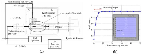
Figure 1.
(a) Schematic of wind tunnel facility; and (b) Mach number profile measured at center plane of M2.0 facility-nozzle exit.
The stagnation temperature of the freestream was equal to room temperature at approximately 281 K. The total pressure of the cell nozzle flow was maintained at a constant preset value, whereas the stagnation pressure of the Mach 2.0 freestream gradually decreased from approximately 200 kPa to 100 kPa. The pressure data measured at the point where static pressure at the M2.0 facility nozzle exit (Pa) matched the test chamber pressure (Pb) were used. Other details of the experiments have been described by Takahashi et al. [12].
2.2. Aerospike Nozzle
Figure 2a presents the aerospike nozzle model and a carefully designed contoured ramp (called a spike) used as the test model. The full-length spike model is shown here, with the projected right view of the duct from the downstream direction being presented on the right. A non-clustered 2D primary nozzle (called a cell nozzle) with a design Mach number of 3.5 was used. The cell nozzle exit plane was connected to the 77 mm straight section and the subsequent spike section. The length of the straight section was determined based on the fact that the contoured section starts at a certain distance from the cell nozzle exit where the first Mach wave emanating from the cell nozzle lip (i.e., top edge of the nozzle exit in Figure 2a) interacts with the bottom surface of the straight section. The contour of the spike was designed using the method of characteristics, resulting in a full length of 196 mm and a height of 57.5 mm. Figure 2b presents the contour geometries of the cell nozzle and the spike nozzle. Gaseous nitrogen (GN2) was used for the cell nozzle flow. Acrylic glass windows located on both sides of the test model served as side fences and provided a 2D Mach 2.0 flow to the spike surface and also enabled optical access as shown in Figure 2a.
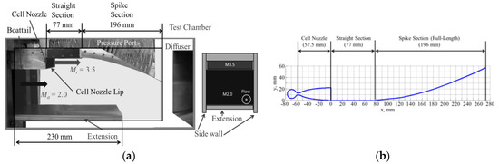
Figure 2.
Geometric schematics used in the experiment, photograph of experimental setup for the full-length spike model, and contour geometries; (a) photograph of experimental model setup; and (b) contour geometries for 2D cell and spike nozzles.
The contour of the 2D cell nozzle was in the vertical direction in which the exit height, width, and throat height were 22 mm, 100 mm, and 2.95 mm, respectively. Above the nozzle, a plate of 2.5 mm thickness was attached as the upper wall (shroud) of the cell nozzle. A pitot-probe survey was conducted separately to investigate the cell nozzle exit Mach number distribution in the vertical direction at the center plane (y = 50 mm). The mean Mach number was found to be approximately 3.50 [12]. The boundary layer thickness was approximately 2.0 mm for the cell nozzle flow. The core region was dominant compared with the boundary layer thickness. Therefore, post-processing of the experimental results and the analytical study will be implemented by assuming that the core flow region dominates the flowfield. The designed nozzle pressure ratio (NPR) values for the cell nozzle and the spike nozzle under optimal expansion conditions were 76.3 and 596.0, respectively.
Wall static pressures were measured using an electric scanning pressure measurement system (PSI ESP-64-HD, Pressure Systems Inc., Phoenix, AZ, USA) at a sampling frequency of 10 Hz. There was a total of 126 pressure ports, with 49 on the straight section and 77 on the spike section. The ports were located on the grid at intervals of 10 and 12.5 mm in the x- and z-directions, respectively. The test chamber pressure was measured inside the test chamber. The total pressure for the Mach 2.0 freestream and GN2 cell nozzle flows were measured separately using strain gauge pressure sensors and then synchronized using the pressure measurement system. As the surface pressure distributions were measured at a sampling frequency of 10 Hz, every value presented hereafter is the averaged value for a duration of 1 s corresponding to 10 sampling points when the NPR attained stability under the target condition. The error bar is the standard deviation (1σ) for the averaging duration.
2.3. BOS Measurement System
2.3.1. Basic Concept of BOS
The basic principle behind visualizing the density gradient field using the refractive index is given by the Gladstone–Dale relationship, which relates density (ρ) with the refractive index (n) as follows [1,7,10]:
The value of the Gladstone–Dale constant G(λ) is assumed to be that of air (0.023 × 10⁻³ m3/kg) throughout this study. The deflection of light contains information on the spatial gradients of the refractive index integrated along the line-of-sight path. Assuming a 2D flowfield, the image deflection (ε) can then be defined as follows:
Based on the geometric relationships depicted in Figure 3, which also covers the current setup, virtual image displacement Δy′ projected on the background screen is related to image displacement Δy captured on the imaging plane of the acquisition system (i.e., camera lens) through the relationship between ZB, ZD, and Zi, assuming that distance Zi is approximately equivalent to focal length f. Using simple trigonometry relations for angles A and B, and assuming that ε is very small (less than 0.1°), thereby also making B small, Δy can be rearranged as follows:
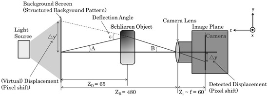
Figure 3.
Schematic of background-oriented schlieren (BOS) principle and setup.
Thus, the deflection of light ray ε is related to key geometrical parameters f, ZB/ZD, and Δy.
In rearranging Equations (1)–(3) by accounting for the displacement directions through an expansion to two dimensions, yields the following second-order elliptic partial differential equation (known as Poisson’s equation) having density field ρ as its solution. The equation is solved numerically using an iterative method such as the successive-overrelaxation method with proper boundary conditions. Boundary conditions and the coefficient (R) on the right side of Equation (4) are discussed in detail in a later section.
2.3.2. BOS Setup
Figure 3 illustrates the BOS setup and the relationship with geometrical distance. The setup consisted of the minimum required key components: an imaging system comprised of a digital charge-coupled device (CCD) camera with an appropriate lens and a background pattern illuminated by a light source. Each setup parameter was carefully determined to ensure adequate sensitivity for deriving Δy from Equation (3) because the sensitivity determines the minimum detectable displacement or pixel shift in the background pattern for a given flowfield. The background screen containing the background pattern was placed on the side window [12].
Although a longer focal length is desirable for lens selection, to detect smaller pixel displacements, a smaller focal length can be compensated for by using a camera with higher spatial resolution. In this study, a lens with a focal length of 60 mm was used to capture the area of interest, in line with the parameters listed in Table 1. The lens was mounted on a commercially available 12 MP class digital CCD camera (D700, Nikon Inc., Minato-ku, Tokyo). The minimum dimension detectable by the CCD sensor chip is 8.46 × 8.44 μm/pixel. The background pattern was determined so as to capture the flow scale of interest, given that interaction between the cell nozzle jet flow and external flow would have dimensions on the order of millimeters. The background pattern consisted of a binary, random, and equally spaced dot pattern with a spatial resolution of 2000 × 2000 pixels printed on A4-sized (210 × 297 mm2) paper with one dot for every 105 × 149 μm/pixel. Because the dimension of the background dot pattern is adequately small but larger than the minimum dimension detectable by the CCD sensor, it is possible to resolve the flow structure of interest. A combination of black and white colors was employed in the binary dot pattern, so as to provide higher contrast than any other combination based on color theory. A commercially available LED light rated at 750 W was used as the illumination source. To maintain the desired sensitivity and account for the area of interest, distance ZB was set as the minimum distance (480 mm) allowed by the experimental configuration and the wind tunnel facility.

Table 1.
Summary of parameters for the BOS measurement system.
Considering that shutter speed, aperture, and ISO sensitivity are closely related to each other, the shutter speed was 1/4000 s in this study to obtain sharper BOS images. The ISO sensitivity was set to 200, which is the minimum value needed to ensure reduced image noise. The aperture (a) was chosen as F4 to nominally focus on both the background pattern and flowfield, as well as to adjust the brightness. Table 1 lists all the parameters of the BOS setup.
2.4. BOS Post-Processing
This section briefly describes the post-processing procedure of BOS. To derive the BOS displacement field by correlating two images, the minimum quadric differences (MQD) algorithm was used with MATLAB in-house code. This algorithm achieves lower correlation errors under nonuniform illumination than the conventional cross-correlation algorithm [18]. The geometrical distortions between both images due to the wind tunnel start-up process were corrected before the correlation processing. The interrogation window size was determined to be 16 × 16 pixels using the three resultant recursive steps, starting from 64 × 64 pixels, with an overlap of 50%. The specified size was found to provide the lowest displacement field error [11]. The spatial resolution in the displacement field is limited by the interrogation window size of 16 × 16 pixels corresponding to 0.80 × 0.80 mm2. To reduce stray vectors in the resultant displacement field, five pairs of images were averaged in each post-processing. Because BOS visualization in this study using the 2D nozzle model only provides line-of-sight-integrated density gradient information, a calculated displacement field only indicates the line-of-sight-integrated flow structure.
2.5. Computational Fluid Dynamics and Code Validation
The aerospike nozzle flowfield that corresponds to the experimental setup was simulated by a computational fluid dynamics (CFD) simulation. JAXA developed the CFD simulation tool at its Kakuda Space Center based on commercially available source code: Open source Field Operation And Manipulation (OpenFOAM) [19]. OpenFOAM has been earning a reputation for facilitating flexible customization for the flowfield of interest and offering robust calculation.
The computational accuracy was validated [19] by comparing the spike surface pressure distribution with that found by the experiment for the same configuration and flow conditions. The flow conditions were the same as those in the current experiment described above, and the NPR for this calculation was 49.5. The CFD calculation for validation was made for a steady two-dimensional flowfield. The rhoCentralFoam with the Tadmor scheme was mainly employed to calculate a supersonic flowfield. It should be noted that a boundary layer thickness of approximately 5 mm was observed on the spike surface in the experiment. Compared to this boundary layer thickness, the core flow region where inviscid flow can be assumed is dominant over the viscous boundary layer thickness. Moreover, since no strong shock-boundary layer interaction was seen in the flowfield of interest which would enable inviscid computation [20,21], inviscid computation was implemented in this study. Note that this assumption would involve some uncertainty that would be arisen from the viscous effect as Bonelli et al. [16,17] presented that the effective viscosity may be affected by strong compressibility, and hence accounting for the viscosity and the compressibility effects on the effective viscosity change would improve the computational accuracy. The computational results with using the inviscid model will be discussed along with theoretical modeling in a later section.
The computation was implemented progressively by changing the initial conditions and entering parameter values via several steps. First, lower values for the flow condition were given as input parameters. For example, 30% of the final desired velocity value was given to the computation. The output flowfield after convergence was used as an initial condition for the next step of the calculation. The flow conditions were slightly increased from those used in the first calculation (e.g., 50% of the desired velocity value). These steps were iterated until the initial conditions and final output values converged. This progressive method facilitates stable and robust calculation for an extreme environment such as seen in high-supersonic to hypersonic flowfields involving a high Mach number and high-pressure flow conditions [19].
For numerical simulation in this work, an adopted mesh grid was utilized so that the computation could resolve multiple complex flow characteristics such as jet shear layer, shock waves, and jet interactions. Figure 4 presents the overall grid used for the CFD simulation to compute the aerospike nozzle flowfield that corresponds to the experimental flowfield. There was a total of 13,040 grids. The minimum grid resolution was 0.1 mm. The specific heat ratio was 1.4, and the gas constant was 287.1 J/(kg·K) as airflow was assumed throughout this study.
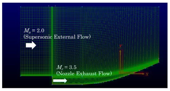
Figure 4.
Mesh grids used for calculation of the aerospike nozzle flowfield. The flow direction is from left to right. The region of interest for computation is the area indicated by the grid.
3. Results and Discussion
This section discusses the insights gained from the BOS post-processing and covers the following topics of interest: qualitative observation of the flowfield and quantitative evaluation of the BOS method deriving the density field by comparing with the results obtained by CFD and the analytical model.
3.1. Qualitative Evaluation of the Flowfield
Figure 5 presents a raw background image (with only external flow) paired with an experimental image (with both external and cell nozzle flows). The background image (Figure 5a) served as the reference from which the pixel displacement corresponding to the density gradient was calculated. In this case, to investigate the interactions between the two types of flow, the background image was chosen as one with only external flow, whereas the experimental image was chosen as one containing both external and cell jet flows. The resultant displacement field represents the region where interactions between external and jet flows were dominant. The images were collected from a single experimental run and saved at 8 bit pixel depth. The displayed images show the cell nozzle exit (at the bottom-left side), the straight section (horizontal line at the bottom) that ends at approximately x = 1200 pixels, and the following spike section. The flow direction is from left to right. As a commercially available non-calibrated work light was used, slight nonuniformity in illumination brightness can be seen (such as the right-side end being darker than other areas in the image). It should be noted that it is not necessary to correct nonuniformity in illumination brightness as long as the background pattern can be identified so as to calculate the pixel movements in the post-processing. The post-processing procedure is described in the previous section. Five pairs of images were averaged to reduce stray vectors. The error displacement is approximately 1 pixel.
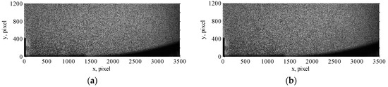
Figure 5.
Raw single-shot images: (a) Reference (background) image (with only external flow); and (b) experimental image (with both external and cell nozzle flows). The figure shows the case of an overexpansion condition, with the flow direction from left to right.
Figure 6a,b presents the flow structure of a representative BOS flow visualization result in the x-direction and y-direction, respectively. The 2D nozzle and full-length spike model were used for BOS visualization as both only include line-of-sight-integrated density gradients; consequently, a calculated displacement field indicates the line-of-sight-integrated flow structure. The case of an overexpansion condition (NPR = 49.5 for cases with external flow) is presented here as an example and as a reference case. Those images were generated by averaging five image pairs from testing under stable wind tunnel operating conditions. The wall surface is presented as a black solid area. The color bar represents the magnitude of pixel displacement between the background and experimental images presented for the purpose of identifying the flow structure. As mentioned before, the pixel displacement physically interprets the density gradient. Therefore, the higher-value region represents areas with stronger density gradients in both the x- and y-directions. The directions in which the density gradient occurred can be identified by displaying the displacement field in the desired direction.
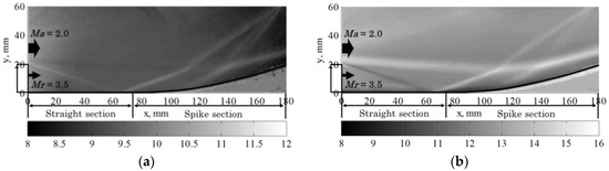
Figure 6.
Displacement field obtained by BOS (a) in the x-direction; and (b) in the y-direction. The flow direction is from left to right, and the color bar indicates pixel displacement.
The displacement field in this flowfield is seen to be dominant in the y-direction compared with the x-direction. Although some error vectors due to background noise, such as those in the external flow region, are observed, noticeable flow structures representing an overexpansion jet consisting of an oblique shock wave emanating from the cell nozzle lip and its reflection on the wall, the jet boundary, double oblique shock waves emanating from the vicinity of the spike entrance, and their interactions are clearly obtained. An expansion fan emanating from the cell nozzle lip is also slightly evident. The most notable feature is the strong jet boundary along the spike wall, which appears as almost parallel to the wall surface. Those characteristic features are similar to those observed in tests with a straight ramp [11]. A slip surface and double oblique shock waves control the jet expansion by pressing the jet boundary against the wall and forcing the jet to remain on the wall surface.
In the next process, the quantitative density field will be discussed. The quantitative density field can be obtained based on those displacement fields and by solving Poisson’s equation as a boundary condition problem. In order to evaluate a proper boundary condition as the wall boundary condition, the following section describes the efforts made for modeling the pressure and density distributions on the spike wall surface.
3.2. Modeling of Spike Wall Pressure and Density Distributions
The boundary condition is crucial to obtaining a proper solution of Poisson’s equation as the boundary condition problem. Among the four boundaries in the region of interest, the most complex boundary—the wall boundary condition—was predicted by the analytical model. The other boundary conditions are described later, in detail.
In order to predict the spike wall surface pressure and density distributions, three approaches were implemented using an analytical model, CFD, and a simplified isentropic assumption based on the measured wall pressure distribution. Although the previous report [12] only described how to derive the distribution of pressure by accounting for the freestream effect, this study has made slight modifications to the model so that it can predict the Mach number and density distribution on the wall. This paper presents brief description of the modified analytical model and presents only the resultant wall surface distribution relative to the density. In addition to the pressure, Mach number, and density on the spike wall predicted by using the analytical model, the wall surface pressure and density distributions obtained from CFD and the simplified isentropic assumption will be given. The wall pressure distribution obtained by the measurement was used to validate the CFD code.
3.2.1. Analytical Model
The pressure, Mach number, and density distributions on the spike surface were predicted using the physics-based analytical model shown in Figure 7, accounting for the plume physics under the presence of the external flow. The flowfield modeled and presented here corresponds to the over-expansion condition. On the basis of quasi-one-dimensional analysis of the flowfield, the flow properties in each categorized zone (shown in Figure 7) were derived.
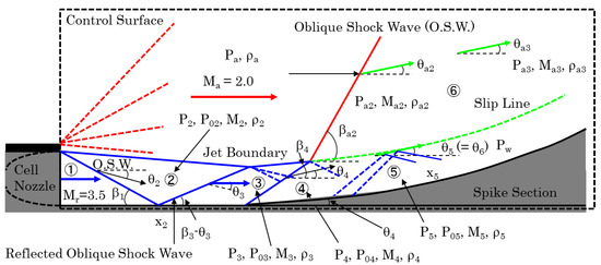
Figure 7.
Schematic of the flowfield model with external flow, under the over-expansion condition of jet. This figure is a modified flowfield model of that available in Reference [12].
The calculation steps are described below. The flow properties were derived for the control surface (expressed as the dotted area in Figure 7) separately with respect to the cell jet flow and external flow. The assumptions made for this modeling are summarized below:
- (1)
- The Mach number of the external flow entering the spike nozzle surface is 2.0.
- (2)
- The Mach number of the cell nozzle jet at its exit is 3.5.
- (3)
- The specific heat ratio γ is constant at a value of 1.4 throughout this study because all the flows are non-reactive.
- (4)
- The entire flowfield is two-dimensional.
- (5)
- The flow properties change isentropically except in the region of a shock wave.
- (6)
- No energy loss occurs due to either skin friction or passing through of oblique shock waves on the wall surface.
- (7)
- The static pressures and flow angles of the cell jet and external flows are the same across the slip surface.
Under these assumptions, the flow properties in each categorized zone illustrated in Figure 7 were derived using the following procedure. Note that regions 1 to 4 represent jet-dominant regions, and regions 5 and 6 represent external-flow-dominant regions. If the flow is under-expanded, the oblique shocks in regions 1 to 3 are replaced with Mach waves. Figure 7 is a modified flowfield model of that available in Takahashi et al. [12].
In regions 1 and 2, Mach numbers, local static pressures and pressure ratios, and local density and density ratios across an oblique shock wave were derived using the following equations with the parameters Mr, static pressure at the cell nozzle exit P1 and the pressure behind the oblique shock wave P2, and the density at the cell nozzle exit ρ1. The value of P2 is treated as a variable because its actual value at the time of calculation may be different owing to the local reduction in pressure due to the formation of the expansion fan from the shroud base as a result of the external flow.
Because the streamline in region 3 after the reflected oblique shock wave must be parallel to wall of the straight section, the following relationship with respect to the flow angle must be retained:
Using β1 obtained from Equation (5), θ2 from Equation (6), and θ3 from Equation (8), the flow properties in regions 2 and 3 were derived using the following relationships:
Thus, the flow properties across every region and the pressure ratio and the density ratio across each oblique shock wave were derived. In region 4, the flow with Mach number M3 and pressure P3 is compressed by the spike entrance, and hence the resultant flow-turning angle due to the initial compression is the same as the initial spike angle (θ4). In this study, θ4 = 5.3° as that given by the spike geometry. The flow properties in region 4 were derived using the following relationships:
Since the spike surface acts as a continuous compression wall, the flow properties between regions 4 and 5 are assumed to change isentropically, and those in region 5 with respect to the cell jet flow are derived by following Prandtl–Meyer relationships:
Here, the local flow turning angle θ5 was assumed to be the same as the local contour angle of the spike geometry. From these equations, Mach number M5 is derived and thus P5 and ρ5 are derived by following isentropic relations. The spike surface pressure P5 and the density ρ5 will be the final output in this process.
For the external flow, the pressure in region 6 was derived as Pa2 (=P6) using the following shock wave equation, with the assumption that the flow turning angle across the oblique shock wave is the same as that of the initial contour angle:
The pressure ratio across the oblique shock wave Pa2/Pa is obtained from Equation (27), and hence Pa2 is obtained. Then, assuming that the flow angles of two streams across the slip line are the same and the flow is compressed gradually along the contoured surface, this yields the following relationships:
Solving Equations (5)–(32) by iterating with respect to the variable P2 until P5 equals P6 (or when the difference between P5 and P6 becomes smaller than the error bar range of 10%) in the x = 109–255 mm region, and at the end of the iteration, the wall surface pressures and densities in each region of the closed control surface in Figure 7 were determined.
In order to quantitatively ensure the calculation accuracy, Figure 8 compares the spike wall surface pressure distribution for the aforementioned flow conditions obtained from the experiment, the physics-based analytical model, and CFD. The wall surface pressure distribution for the case of NPR = 49.5 is presented. Some discrepancies between the experiment and the analytical model are attributable to the fact that the analytical model was based on quasi-one-dimensional theory and did not account for the oblique shock wave emanating at around x = 110 mm, whereas the experiment involved two-dimensional flow features and some three-dimensionality as well. The CFD result shows better agreement with the experimental data than the analytical model. A slight discrepancy between the experimental and CFD results is still seen. One of the cause of this discrepancy is attributable to how the CFD computation was implemented with inviscid model as described in Section 2.5. Although more accurate computation would be expected by the CFD with viscous model, the discrepancy between the experimental and CFD results is within the error bar obtained from the experiment. Thus, the CFD simulation tool developed in this study sufficiently and accurately reproduced the spike wall surface pressure distribution both qualitatively and quantitatively, thereby verifying its accuracy in reproducing the flowfield. Moreover, the analytical model can adequately predict the wall pressure distribution except in the oblique shock region around x = 110 mm, and thus it can predict the density and Mach number distributions.
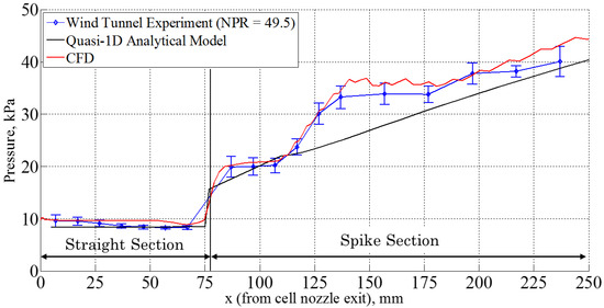
Figure 8.
Comparison of spike wall pressure distribution among the experiment, analytical model, and computational fluid dynamics (CFD). The nozzle pressure ratio (NPR) was 49.5 and the external flow Mach number was 2.0.
3.2.2. Simplified Isentropic Assumption
In cases where establishing an analytical model cannot easily predict flow properties due to the complexity of the flowfield, a simplified alternative method was devised to estimate the wall pressure and density distributions using measured wall pressure data under the isentropic assumption. As the wall pressure distribution can be measured relatively easily, the isentropic relationship was used to estimate the density distribution from the measured pressure distribution. It should be noted that the isentropic assumption generally collapses where a shock wave exists because its presence causes total pressure losses. Therefore, the isentropic assumption for this complex flowfield involves some uncertainties due to the total pressure loss. The wall density distribution was estimated by accounting for such uncertainties.
The wall density distribution can be estimated by Equation (33). Here, and are total pressure and density at the cell nozzle exit, respectively, and and are the total pressure and density accounting for their loss due to the presence of a shock wave, respectively. The term with Δ indicates the loss term. The first term in Equation (33) is the pure isentropic relationship between density and pressure. The second term accounts for the total pressure loss () and resultant total density loss (). Here, by considering calorically perfect gas for entire flowfield, the total temperature across the shock waves is preserved; hence, , and this approximation yields the third equation in Equation (33). The uncertainty comes from . Expanding the third term by the binomial theorem yields the fourth term. It is necessary to estimate the uncertainty from the possible range of .
Figure 9 presents the wall Mach number distribution predicted by the analytical model. As seen in Figure 9, the possible Mach number range on the wall is between 2.4 and 3.5 for the entire wall surface, and between 2.4 and 3.2 for the contoured spike surface. Since the density distribution on the contoured spike surface is important here, the Mach number range of 2.4 to 3.2 is considered. Figure 10 estimates the total pressure loss for the aforementioned possible Mach number range in the oblique shock angle and the Mach number in the flowfield of interest. With some margin, can be estimated up to 11% in the form of percentage; therefore, the higher order term in the fourth equation in Equation (33) rather than the third order can be considered as neglected (less than 1 × 10⁻⁴). This yields the following expression with uncertainty Δ ~ 3%.
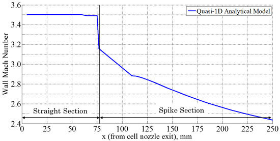
Figure 9.
Spike wall Mach number distribution predicted by the analytical model.
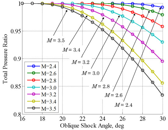
Figure 10.
Total pressure ratios across an oblique shock wave for various Mach numbers.
Thus, an approximate 3% uncertainty will be included in this isentropic estimation of wall density distribution from the measured pressure distribution.
Figure 11 presents the density distribution estimated by this isentropic assumption as well as that derived by the analytical model and CFD. The error bar for the simplified isentropic assumption model is a 3% uncertainty. As seen in this figure, the isentropic assumption can favorably estimate the wall density distribution. Thus, the simplified isentropic assumption based on the measured pressure distribution on the wall can be used with an acceptable level of error. This wall density distribution will be used as the wall boundary condition for solving Poisson’s equation in the next section.
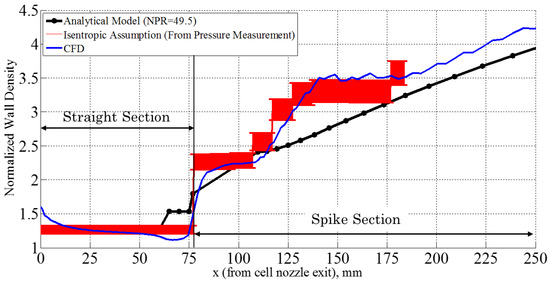
Figure 11.
Comparison of spike wall density distribution among the analytical model, CFD, and isentropic estimation. The NPR was 49.5 and the external flow Mach number was 2.0.
3.3. Quantitative Evaluation
This section discusses the propagation of uncertainty in order to identify the possible uncertainties inherent in the measurement and post-processing, noise sources, and other sources of uncertainty. The possible sources of uncertainty are freestream uncertainty, uncertainty in deriving the vector field from BOS post-processing, uncertainty in setup, and boundary conditions and coefficients that appear in the post-processing. The freestream uncertainty was considered a variation of Mach number during 20 s of wind tunnel operation, and 1σ for the averaging duration was approximately 1.2%. Uncertainties in equipment, setup, and stray noises due to slight ambient air variations are considered to be included in BOS background measurement where two images are measured under a no-flow condition.
Table 2 summarizes each uncertainty source and its value. The total uncertainty obtained for deriving the density field determined by uncertainty propagation is approximately 4.1%.
Table 2.
Summary of uncertainty sources.
As the uniqueness theorem states, it is crucial to give a proper boundary condition to derive a unique solution from solving Poisson’s equation. Table 3 tabulates the boundary conditions of the four boundaries for the region of interest. The left boundary was defined as the entrance condition to the control surface with known values for both flows. The top and right boundaries were considered as the flow-out condition and thus defined by the Neumann boundary condition. As the initial condition, all flowfields other than the boundaries were given as unity. The wall boundary condition is that derived by using the analytical model described in the previous section.
Table 3.
Boundary conditions for Poisson’s equation.
Figure 12 presents the wall boundary distribution showing the sensitivity of coefficient R for solving Poisson’s equation, the solution of which is the density field. Accounting for the physical interpretation of Poisson’s equation, this coefficient R serves as an amplification factor for the solution. The flow condition for this calculation was the same as that given in Figure 8. Density distributions obtained by CFD and the analytical model are also plotted simultaneously for comparison. Obviously, the coefficient R value plays a major role in determining the solution. Note that the coefficient value appearing on the right side of Poisson’s equation, which could be obtained from the experimental setup, was obtained using the “best-fit” approach by comparing the wall density distribution between the BOS and the analytical model. By changing the coefficient value and comparing the resultant wall density to that obtained by the analytical model, the coefficient value was finally determined. In order to obtain an appropriate R value, the least-square fitting of density distributions between the BOS data and the analytical model was given, and the R value of 0.1 was found to facilitate the best solution with less uncertainty or less discrepancy between BOS and the analytical model. Thus, the present method is useful, and the R value of 0.1 will be used in later analysis of this flow condition.
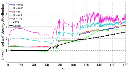
Figure 12.
Sensitivity of R on the density calculation by solving Poisson’s equation.
Figure 13 compares the flowfield characteristics relative to the flow structure around the aerospike nozzle in the presence of Mach 2.0 external flow. The color bar represents the normalized density based on the density value obtained in the freestream region. Jacobi’s method (a relaxation (iterative) method) was used to numerically solve the equation. The conversion was judged when the maximum difference in the entire ROI for the i-th step and (i + 1)-th step in the iteration becomes 10−5. Qualitatively, the flowfields obtained by the experiment (Figure 13a) and by CFD (Figure 13b) match each other in that a remarkable flow structure such as a double oblique shock wave, jet boundary, slip surface, or expansion wave appears.
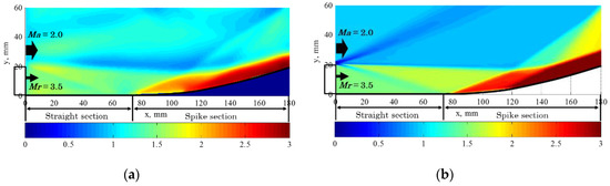
Figure 13.
Comparison of qualitative flowfield features between the experiment and CFD for nozzle pressure ratio (NPR) = 49.5 and Mach 2.0 flight condition: (a) Density distribution obtained by the experiment using BOS; and (b) density distribution obtained by CFD calculated for aerospike nozzle flowfield corresponding to the experimental model. The flow direction is from left to right, and the color bar represents the normalized density based on the density value in the freestream region.
3.4. Application to other Conditions
In order to explore the applicability of density derived with the simplified isentropic assumption, the method was applied to another case without external flow (M∞ = 0). Figure 14 shows the derived density field (a) and its wall distribution (b). The NPR is 35.0 in this case. Similar to the case with a supersonic external flow, the wall density distribution was obtained by assuming an isentropic relationship with the measured pressure distribution on the wall. The R value was found to be 0.10. The shock structure associated with the cell nozzle jet is clearly seen in Figure 14a. The wall density distributions derived from BOS and the isentropic assumption agree well as seen in Figure 14b. Thus, the current approach with a simplified isentropic assumption can be applicable to other cases as well as the reference case.
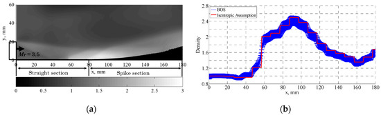
Figure 14.
(a) Density field (flow direction left to right); and (b) wall density distribution when NPR = 35.0 without external flow.
4. Conclusions
A practical approach for deriving the absolute density field based on the background-oriented schlieren (BOS) method in high-speed flowfields was evaluated. The post-processing procedure for determining the coefficient appeared on the right side of Poisson’s equation used to solve the density field, and the wall boundary conditions were evaluated with some assumptions, as both factors play a major role in deriving an appropriate density field. The flowfield of interest was a compressible flowfield consisting of two supersonic flows that could be seen in the aerospike nozzle flowfield. The qualitative feature of the flowfield was consistent with that derived by the BOS technique, and the quantitative feature (particularly in wall density distribution) agreed well among CFD and the experiment with a simplified isentropic assumption. As wall pressure measurement involves less complexity than wall density measurement, the current approach for approximating the wall density distribution to be used as the boundary condition for Poisson’s equation is taken from the measured wall pressure with the isentropic assumption. Thus, the current approach is practical for deriving the absolute density field based on the BOS technique.
Author Contributions
H.T. is responsible for the entire work from conceptualization, conducting experiments, establishing methodology, data analysis, and writing the original manuscript entirely.
Funding
This research received no external funding.
Acknowledgments
The author wishes to thank Shigeru Sato of the computational group at the JAXA Kakuda Space Center for providing the computational environment, and Toshihiko Munakata at Hitachi solutions east Japan Ltd., for developing the computational simulation tool. The author also wishes to acknowledge staff members of the group and experimental facility for their help in conducting the experiment.
Conflicts of Interest
The author declares no conflict of interest.
Nomenclature
| f | focal length, mm |
| M | Mach number |
| NPR | nozzle pressure ratio defined as P0r/Pb |
| n | refractive index |
| Pa | static pressure of freestream, kPa |
| Pb | static pressure in the test chamber, kPa |
| P0r | total pressure of the cell nozzle flow, kPa |
| Pr | static pressure at the cell nozzle exit, kPa |
| Pw | static pressure on nozzle surface, kPa |
| T | temperature, K |
| W | width of schlieren object, mm |
| x | coordinate axis in streamwise direction |
| y | coordinate axis in perpendicular to flow direction |
| z | coordinate axis in line-of-sight direction |
| β | oblique shock wave angle, rad |
| ε | image deflection |
| γ | specific heat ratio (=1.4) |
| ρ | density, kg/m3 |
| θ | angle, rad |
| Subscripts | |
| 0 | stagnation or reference condition |
| a | ambient or freestream condition |
| b | environmental condition |
| r | cell nozzle flow condition |
References
- Settles, G.S.; Hargather, M.J. A Review of Recent Developments in Schlieren and Shadowgraph Techniques. Meas. Sci. Technol. Top. Rev. 2017, 28, 042001. [Google Scholar] [CrossRef]
- Hargather, M.J.; Settles, G.S. Natural-Background-Oriented Schlieren Imaging. Exp. Fluids 2010, 48, 59–68. [Google Scholar] [CrossRef]
- Raffel, M. Background-Oriented Schlieren (BOS) Technique. Exp. Fluids 2015, 56, 145–160. [Google Scholar] [CrossRef]
- Hargather, M.J.; Settles, G.S. A Comparison of Three Quantitative Schlieren Techniques. Opt. Lasers Eng. 2012, 50, 8–17. [Google Scholar] [CrossRef]
- Meyer, G.E.A. Computerized Background-Oriented Schlieren. Exp. Fluids 2002, 33, 181–187. [Google Scholar] [CrossRef]
- Venkatakrishnan, L. Density Measurements in an Axisymmetric Underexpanded Jet by Background-Oriented Schlieren Technique. AIAA J. 2005, 43, 1574–1579. [Google Scholar] [CrossRef]
- Venkatakrishnan, L.; Meier, G.E.A. Density Measurements Using the Background Oriented Schlieren Technique. Exp. Fluids 2004, 37, 237–247. [Google Scholar] [CrossRef]
- Hartmann, U.; Adamczuk, R.; Seume, J. Tomographic Background Oriented Schlieren Applications for Turbomachinery. In Proceedings of the 53rd AIAA Aerospace Sciences Meeting, Kissimmee, FL, USA, 5–9 January 2015. AIAA-2015-1690. [Google Scholar]
- Goldhahn, E.; Seume, J. Background Oriented Schlieren Technique: Sensitivity, Accuracy, Resolution and Application to a Three-Dimensional Density Field. Exp. Fluids 2007, 43, 241–249. [Google Scholar] [CrossRef]
- Bichal, A.; Thurow, B.S. On the Application of Background Oriented Schlieren for Wavefront Sensing. Meas. Sci. Technol. 2014, 25, 015001. [Google Scholar] [CrossRef]
- Takahashi, H.; Tomioka, S.; Sakuranaka, N.; Tomita, T.; Kuwamori, K.; Masuya, G. Influence of External Flow on Plume Physics of Clustered Linear Aerospike Nozzles. J. Propuls. Power 2014, 30, 1199–1212. [Google Scholar] [CrossRef]
- Takahashi, H.; Tomioka, S.; Tomita, T.; Sakuranaka, N. Aerodynamic Characterization of Linear Aerospike Nozzles in Off-Design Flight Conditions. J. Propuls. Power 2015, 31, 204–218. [Google Scholar] [CrossRef]
- Geers, J.S.; Yu, K.H. Systematic Application of Background-Oriented Schlieren for Isolator Shock Train Visualization. AIAA J. 2017, 55, 1105–1117. [Google Scholar] [CrossRef]
- Heineck, J.T.; Banks, D.W.; Schairer, E.T.; Haering, E.A., Jr.; Bean, P.S. Background Oriented Schlieren (BOS) of a Supersonic Aircraft in Flight. In Proceedings of the AIAA Flight Testing Conference, Washington, DC, USA, 13–17 June 2016. AIAA-2016-3356. [Google Scholar]
- Smith, N.T.; Heineck, J.T.; Schairer, E.T. Optical Flow for Flight and Wind Tunnel Background Oriented Schlieren Imaging. In Proceedings of the 55th AIAA Aerospace Sciences Meeting, Grapevine, TX, USA, 9–13 January 2017. AIAA-2017-0472. [Google Scholar]
- Bonelli, F.; Viggiano, A.; Magi, V. A numerical analysis of hydrogen underexpanded jets. In Proceedings of the Spring Technical Conference of the ASME Internal Combustion Engine Division 2012, ASME 2012 Internal Combustion Engine Division Spring Technical Conference (ICES 2012), Torino, Italy, 6–9 May 2012; pp. 681–690. [Google Scholar]
- Bonelli, F.; Viggiano, A.; Magi, V. A Numerical Analysis of Hydrogen Underexpanded Jets Under Real Gas Assumption. J. Fluids Eng. 2013, 135, 121101. [Google Scholar] [CrossRef]
- Gui, L.; Merzkirch, W. A Comparative Study of the MQD Method and Several Correlation-Based PIV Evaluation Algorithms. Exp. Fluids 2000, 28, 36–44. [Google Scholar]
- Takahashi, H.; Munakata, T.; Sato, S. Thrust Augmentation by Airframe-Integrated Linear-Spike Nozzle Concept for High-Speed Aircraft. Aerospace 2018, 5, 19. [Google Scholar] [CrossRef]
- Agon, A.; Abeynayake, D.; Smart, M. Applicability of Viscous and Inviscid Flow Solvers to the Hypersonic REST Inlet. In Proceedings of the 18th Australian Fluid Mechanics Conference, Launceston, Australia, 3–7 December 2012; pp. 3–6. [Google Scholar]
- Ward, A.D.T.; Smart, M.K.; Gollan, R.J. Development of a Rapid Inviscid-Boundary Layer Aerodynamic Tool. In Proceedings of the 22nd AIAA International Space Planes and Hypersonics Systems and Technologies Conference, Moscow, Russia, 21–24 September 2018. AIAA-2018-5270. [Google Scholar]
© 2018 by the author. Licensee MDPI, Basel, Switzerland. This article is an open access article distributed under the terms and conditions of the Creative Commons Attribution (CC BY) license (http://creativecommons.org/licenses/by/4.0/).