Development of an L-Band SAR Microsatellite Antenna for Earth Observation

Abstract

A compact synthetic aperture radar microsatellite antenna operating in the L-band is presented. To reduce size and weight of the small spaceborne SAR, we utilize a lightweight deployable parabolic mesh reflector and operate at low Earth orbital altitudes. The antenna is a wrap-rib center-fed parabolic reflector with dedicated receiving and transmitting feeds. Antenna requirements are: gain better than 30 dBic, center frequency of 1.275 GHz with bandwidth of 28 MHz and circular polarization with axial ratio better than 3 dB. This work describes the development of a compact Circularly Polarized SAR L-band antenna system and the design considerations suitable for small spacecrafts. Simulation of the parabolic reflector and effects of different structural elements to the main radiation pattern were analyzed, which include ribs, struts, feed blockage, and mesh surface. A research model of the parabolic reflector was constructed, and the reflector surface verification was realized using two different approaches, a laser distance meter along ribs and the other using 3D scanning of the reflector surface. RMS errors wree 1.92 mm and 3.86 mm, respectively, both below required 4.55 mm of surface accuracy. Near-field antenna measurements of the deployable reflector mesh antenna was realized for final antenna validation, presenting good agreement with the simulation results. Future work comprises prototyping and testing of the full polarimetric feed assembly.

1. Introduction

1.1. Background on SAR Spacecrafts and Small Satellites

Synthetic Aperture Radar (SAR) technology has been widely used in Earth observation applications, as it can provide unique information independent of cloud coverage and during night time. With the recent miniaturization of technological components, it is nowadays possible to achieve significantly reduced size of payload and bus systems [1]. Constellations of small satellites carrying scientific or commercial payloads provide fast responses and near real-time ground monitoring [2]. Many such satellites carry small payloads as optical cameras or radio receivers, with spacecraft mass ranging from less than a kilogram to few hundred kilograms. However, when it comes to spaceborne SAR, due to mostly the large antenna sizes and high transmission power required, reducing the total spacecrafts mass becomes a very challenging task. Consequently, the bulky payloads and high costs result in SAR missions being commonly sponsored by governmental space agencies. Therefore, up to this date, the number of compact SAR missions with mass of few hundred kilograms are very limited. Moreover, there is a strong social demand to realize small and affordable SAR satellites for fast responses and all-weather monitoring. Such needs are especially important in the Southeast Asian countries, often covered by clouds, which limits observation with optical satellites.

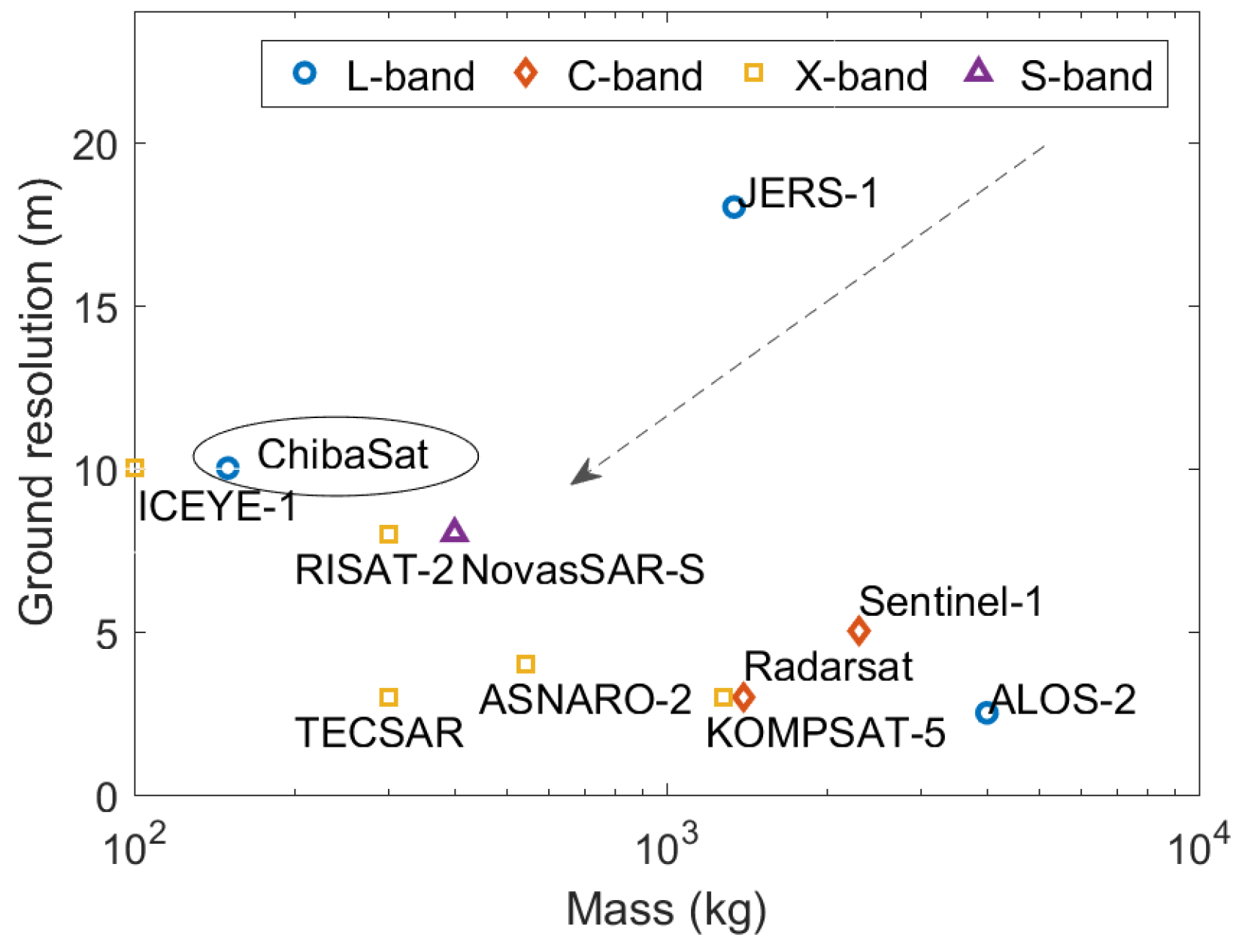
Figure 1 depicts past, existing and future spaceborne SAR missions, relating total spacecraft mass and respective ground resolution, for Noise Equivalent Delta Sigma ${\sigma }_{NE}^0=-20$ dB. For each SAR frequency band, there is a visible barrier in size, performance and, consequently, costs to be able to set up affordable SAR constellations. The miniaturization trend in spaceborne SAR is clearly visible in the high frequency bands, but breaking the ton-sized category is still challenging in the low frequencies, namely in the L-band. While low SAR frequencies may provide unique ground surface scattering information, the very few existing compact spaceborne SAR missions operate in X- or S-bands, as such antennas occupy low volume and are easier to stow. Some examples are the X-band TECSAR (Israel, 300 kg) [3], pioneer in showing that a SAR payload could be flown on smaller satellites, and the recent X-band microsat SAR ICEYE-X1 (70 kg, Finland) [4], launched in early 2018 as a promising proof-of-concept prototype for future planned constellation.

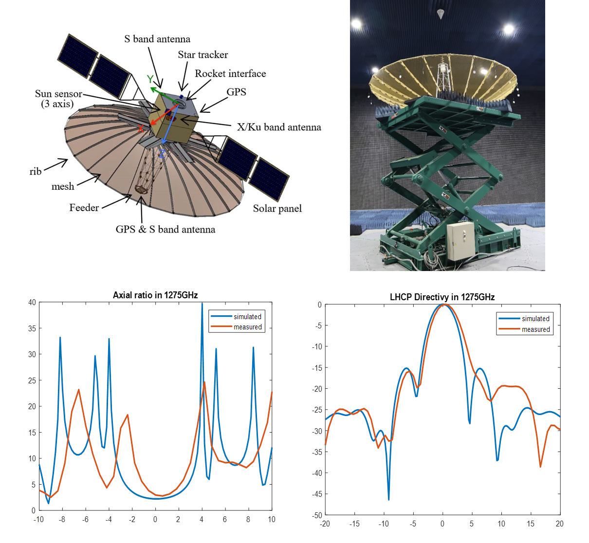
Currently, Chiba University and the Indonesian National Institute of Aeronautics and Space (LAPAN) are developing a monostatic passive L-band SAR microsatellite for Earth observation, as part of a technology demonstrator for small spaceborne SAR systems.

Table 1. Remote sensing applications of the L-band microsat mission.

Application	Detail
Land	Forest classification
	Land deformation
	Paddy field extraction
	Wetland extraction
	Mangrove area mapping
Ocean	maritime traffic
	oil spill
	ocean waves
Cryosphere	Icebergs

describes the considered remote sensing applications covered by the mission. A new concept of a 150-kg-class microsatellite circularly polarized SAR is proposed, composed of a compact L-band SAR payload, allowing for piggy-back launch opportunities for the mission. Main strategies for weight and volume reduction are based on a deployable and lightweight SAR antenna, a compact SAR RF system inherited from an airborne-based system, and the use of a low Earth orbit. A primary goal is to demonstrate basic SAR acquisition, showing that an L-band SAR mission can be performed with a microsatellite, and, therefore, making SAR data more affordable for the global remote sensing communities in the future.

1.2. Motivation for Deployable Reflector Antenna

The SAR antenna is one of the design drivers of SAR platforms. It plays an important role with regards to the final imaging performance, as antenna gain, cross-polarization and side lobe levels (SLL) directly affect the SAR data quality. For the implementation of a small L-band SAR satellite, a lightweight high-gain antenna that occupies low stowage space is the main challenge. Such requirements dictate the adoption of deployable antennas. There are promising ongoing developments on deployable inflatable antennas, but difficulties in controlling gas pressure still poses critical challenges with regards to surface accuracy, and thus deemed not suitable for our requirements. Moreover, reflectarray antennas may offer potential as affordable and light SAR antennas, as recently demonstrated in space onboard Isara cubesat mission [5], but still have limitations with regards to antenna aperture sizes. A common choice for SAR antennas is deployable active phased array antennas, as in the 10 m-long L-band antenna onboard ALOS-2 [6]. However, such antenna types are usually heavy, expensive and with complex design.

On the other hand, reflector antennas are one of the most commonly used solutions for high-gain spacecraft antennas, as they provide high efficiency and can support any polarization. Deployable mesh antenna reflectors have proven to be a venerable product for low frequency communications and radar applications where high gain is required. However, very few scientific missions have successfully adopted deployable reflectors, such as the 6-m large deployable mesh reflector antenna for SMAP (Soil Moisture Active Passive) mission [7,8], with most being extensively used for commercial or military applications [2,3]. Up to date, all flown deployable reflectors have been developed for large spacecrafts, which makes scaling down to microsatellite dimensions not possible, since mesh parameters (density, coating, etc.) are driven by the deployment mechanism elements and RF requirements.

Table 2. Advantages and disadvantages of potential high gain deployable antenna technology concepts for a 150-kg class microsat SAR.

	Active Phased Array	Reflectarray	Mesh Reflector	Inflatable
+	reconfigurable beam	stowage efficiency	good antenna efficiency	stowage efficiency
	controllable SLL	simple deployment mechanism	any polarization	simple deployment
	multi-mode scan	low cost	low mass density	large bandwidth
		low SLL
−	high cost	low antenna efficiency	medium cost	poor surface accuracy
	large stowage	restricted mode	high SLL	high SLL
	large mass density	limited antenna aperture	no scan mode	reliability risk
	complex design		complex deployment

summarizes advantages and drawbacks of various high gain deployable antennas that can be suitable as microsat SAR antennas.

1.3. Motivation for Circularly Polarized SAR

Earth observation spaceborne SAR systems are conventionally linearly-polarized, although there are many benefits of circularly-polarized sensors [9]. Circular polarization has the advantage of minimizing the ionospheric effect known as Faraday rotation, which degrades linearly polarized waves most severely in the frequencies below 1.2 GHz. In addition, the use of circular polarization reduces effects of antenna misalignments and multipath propagation, improving the received signal. Circular polarization is typically used in satellite communication links, but its use in spaceborne SAR systems for remote sensing has not been much explored. The main reason is difficulty in making antenna systems that comply with the strict requirements of circular polarization, such as antennas with almost perfect axial ratio.

In polarimetric SAR, transmitting in circular or tilted linear polarization has gained popularity over the years as it overcomes existing drawbacks in the conventional polarimetric linear polarized SAR, the so-called compact polarimetric or pseudo quad-pol SAR [10]. The drawback is that, although suitable for some key applications, compact SAR data cannot replicate all aspects of full polarimetric imagery.

Recently, a SAR mode that adopts circular polarization signals in transmission while receiving both polarizations has been proposed [9], and its concept referred to CP-SAR (Patent Pending 2014-214905). Application of a ground based full-polarimetric CP-SAR on rice phenology monitoring has been demonstrated [11], showing adequate classification capability of rice paddies. The L-band microsat is designed to support full polarimetric CP-SAR for concept demonstration, but to avoid too large data amounts it should operate mostly in one polarization, that is, transmitting either left-hand-circular polarization (LHCP) or right-hand-circular polarization (RHCP), and receiving both. To guarantee a high degree of circularly polarized scattered waves, the microsat CP-SAR must consider look angles below 50${}^{\circ }$, as up to this angle, the polarization of scattered waves presents axial ratio under 3 dB [9]. Apart from being a technology demonstrator, the microsat’s main mission is to support research on elliptically polarized scattering for remote sensing applications, aiming for the development of end-user products.

1.4. Motivation for Low Earth Orbits

Lowering orbital altitudes is a clear advantage for small sats, as it directly reduces the minimum antenna area that complies with the pulse repetition frequency (PRF) constraints. Power requirements and cross track resolution are also improved in lower orbits [12]. The minimum antenna area $A_{min}$ is a function of orbital height R, incidence angle $\theta$ and platform velocity $v_{st}$, referenced in Equation (1).

$$A_{min}\ge \frac{4v_{st}R\lambda tan\left(\theta \right)}{c}$$

(1)

Additionally, a reduction on the antenna dimensions as much to fit the launcher envelope is mandatory. Therefore, an orbit height as low as possible is advantageous for the CP-SAR microsat. On the other hand, orbital altitudes lower than 500 km are subjected to atmospheric drag, considerably reducing the mission life time. Considering the requirements of the Indonesian and Japanese partners, the investigations concentrate on orbits with height around 500–600 km, accepting a shorter mission life span of at least one year. Therefore, the basis for the SAR sensor design was chosen to be at orbital altitudes of 500 km.

This work presents the main design considerations for a compact SAR antenna, highlighting simulation and validation of the parabolic reflector antenna. Antenna pattern simulations were performed with the full wave simulation software 2018 CST Studio [13]. Simulations and antenna measurements considered a single feed antenna element. Future work shall concentrate in the development and performance verification of the feed assembly, and overall performance integrated with the parabolic reflector.

This document is organized as follows: Section 2 describes the main considerations for the design of the deployable mesh reflector antenna; Section 3 describes the antenna effective gain estimation; Section 4 presents methods for the verification of reflector surface accuracy and subsequent results achieved; and Section 5 concludes with a summary of the current study and an outlook to future work.

2. Deployable Mesh Antenna Design

2.1. SAR Considerations

In a SAR system, the antenna size must be determined at an early stage of the design, as antenna length and width define the half-power beamwidth (HPBW) of the antenna pattern, from which many other SAR parameters are derived.

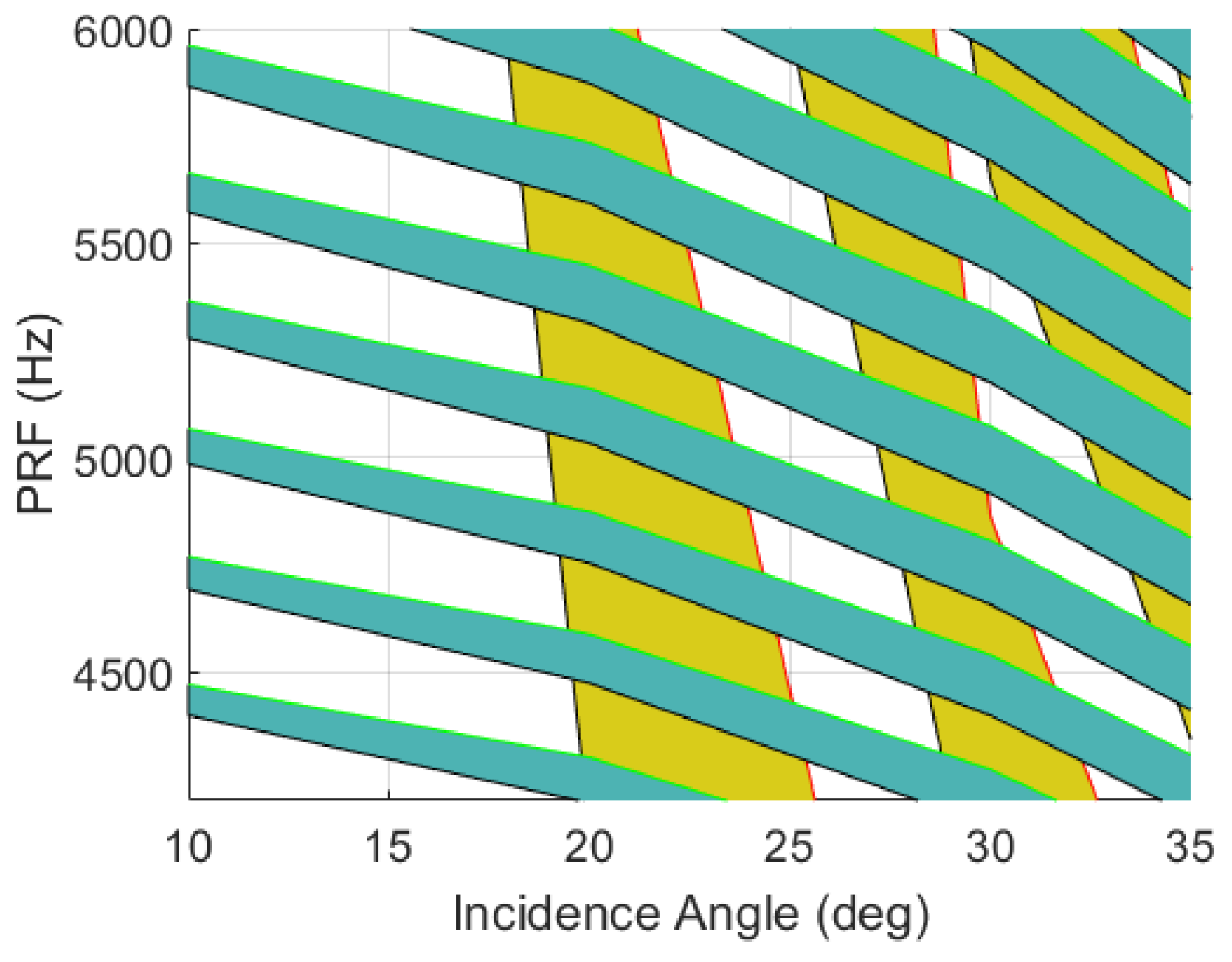
Volume constraints from the launcher envelope allowed a maximum antenna diameter of 3.6 m. This gives a $PR{F}_{min}$ of 4.2 kHz, and defines a range of valid PRFs and subsequent SAR system parameters. When accounting ambiguities from blind ranges and nadir returns, non interference PRF values are limited to 4.2–7.5 kHz within 15${}^{\circ }$–35${}^{\circ }$. That corresponds to an access area of 216 km on both sides of the nadir track. Figure 2 plots usable PRF values (white area) as a function of incidence angle for a 3.6 m-diameter parabolic antenna, accounting eclipsing from transmitter pulse (yellow) and nadir echos (blue). In full polarimetric mode, the PRF must be doubled, leading to a useful range of 8.4–15 kHz. Even for high PRF values, the Ambiguity Signal Ratio (ASR) is below −18 dB considering targets with uniform reflectivity. For transmission peak power of 1500 W, ground resolution of 30 m with a standard image quality NESZ of −20 dB can be achieved from 500 km altitudes. Swaths of 15–30 km wide can be achieved to cover the remote sensing applications considered for the mission, as listed in Table 1. That way, at the cost of smaller swath widths, a 3.6 m diameter sized antenna in combination with low orbit would allow good SAR sensitivity with reasonable power budget. A summary of the mission and antenna’s specifications can be seen in

Table 3. Mission and antenna specifications.

Mission Parameter	Specification
Altitude	500–600 km
Orbit	sun-synchronous polar
	inclination of 97.6${}^{\circ }$
SAR Modes	stripmap, spotlight
Coverage	Japan, Indonesia
Frequency	L-band (1.275 GHz
	85 MHz bandwidth)
Polarization	transmit LHCP/RHCP
	receive LHCP+RHCP
Spatial resolution	10–30 m
Swath width	15–30 km
Look angle	20${}^{\circ }$–35${}^{\circ }$
Bus Size	80 cm × 80 cm × 85 cm
Total mass	<150 kg
Transmitting power	800–1500 W
Duty cycle	10 %
PRF	4.2–5 kHz
NESZ	<$-20$ dB
ASR	<$-18$ dB
Chirp Pulse	10–20 $\mathsf{\mu }$s
Gain	>30 dBic
Polarization	LHCP and RHCP
Surface accuracy	<4.22 mm RMS
Axial ratio	>3 dB
Side lobe level	>20 dBic
Stowed size	0.85 m × 0.85 m × 1.3 m
Deployed size	3.6 m × 0.65 m (depth)
Total mass	<15 kg

.

Next, details of the design of the parabolic reflector antenna are discussed.

2.2. Antenna Configuration

Among the different types of reflector configurations, a primary center-fed parabolic type was chosen. Other reflector configurations were considered, but they would either present more complex design or not satisfy the CP-SAR requirements. For instance, having an offset feed could avoid feed blockage, but at the cost of decrease of CP signal purity and increased design complexity of the deployment mechanism; a L-band Cassegrain configuration could significantly improve feed illumination efficiency but would require a too large subreflector, posing a problem in terms of volume constraints and signal purity. Hence, aiming for a simple configuration suitable for the system specifications, a primary-fed parabolic configuration was chosen. Careful feed design to minimize feed blockage achieving desired level of signal purity is then required for optimum performance.

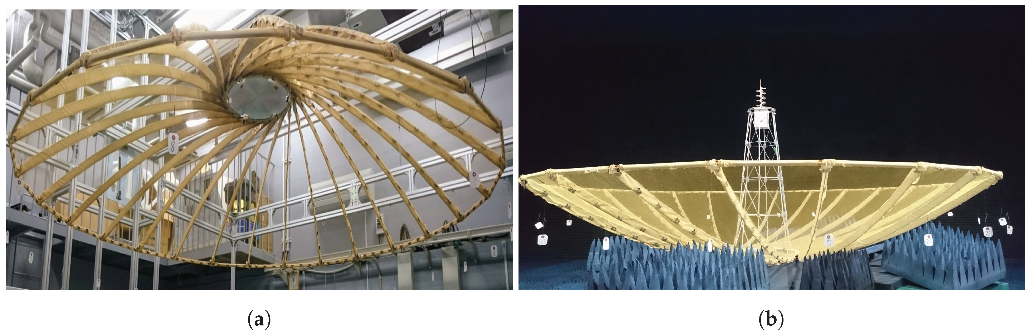
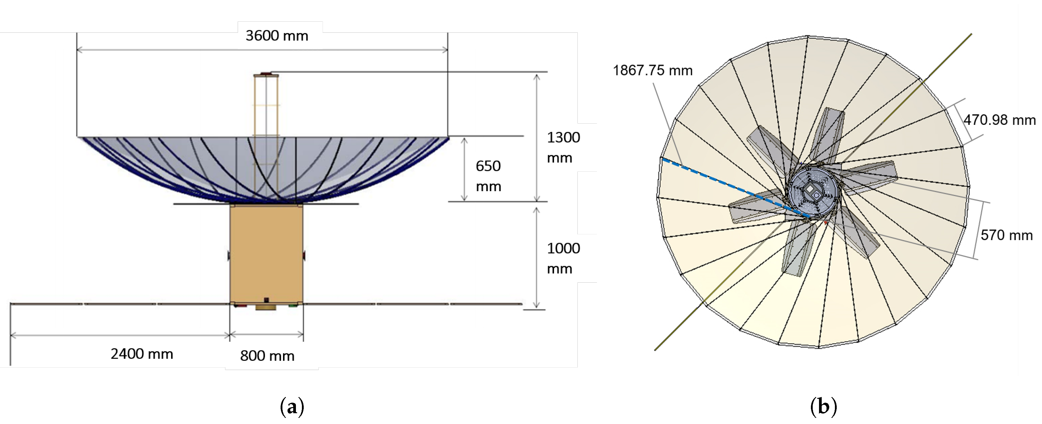
The antenna system consists of the following elements: feed assembly, comprising of switchable LHCP and RHCP receiving and transmitting antennas, six aluminum support struts, and a parabolic reflector, composed of 24 ribs, a solid aluminum center plate and thin mesh layer covering the rest of the surface. Figure 3a,b illustrates the deployable antenna. The fairing space limited the parabolic focal distance to $f_d=1.3$ m, resulting in f/D parameter of 0.363. The deployable reflector’s total weight is 15 kg, with dimensions of 3.6 m (diameter) by 0.65 m (depth) when deployed, and 0.85 m (length) by 0.85 m (width) by 1.3 m (height) when stowed.

Since the sensor has no electronic beam steering, the whole satellite must be rolled in the necessary position for pointing to the desired target.

2.3. Feed Antenna

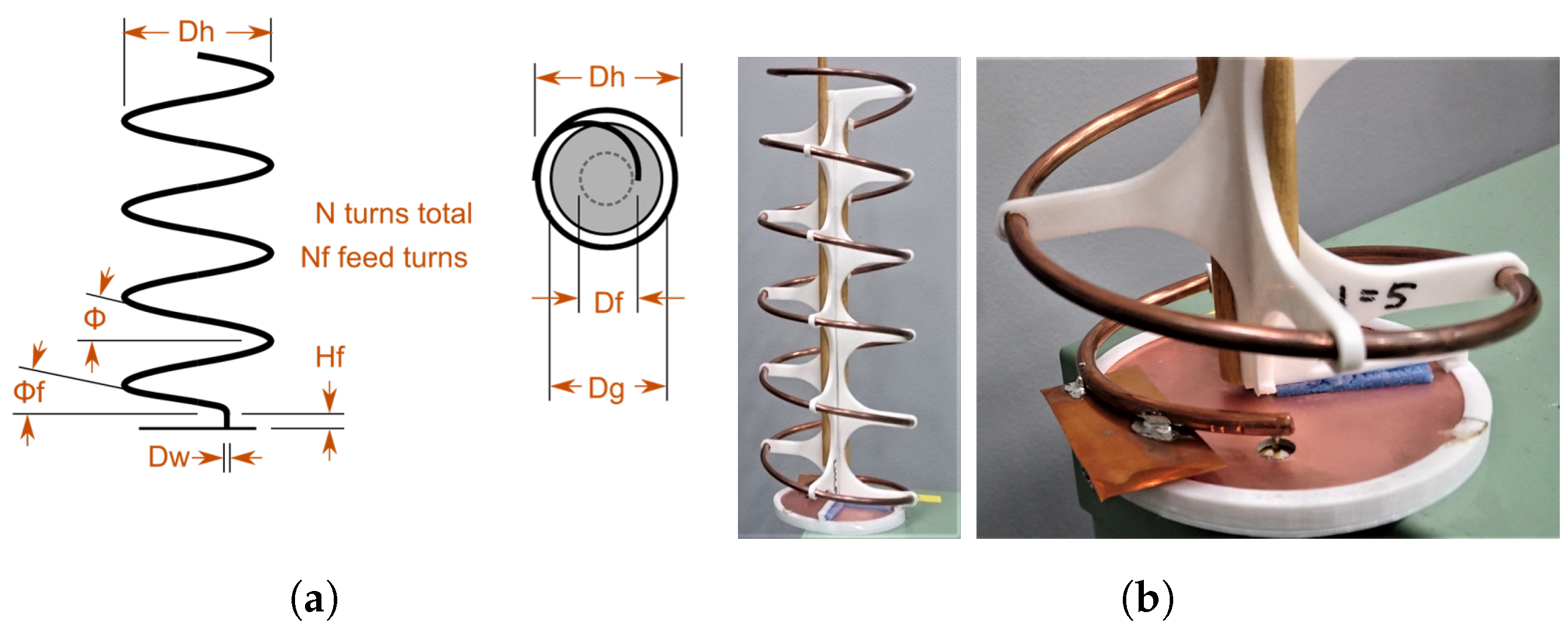
The feed assembly comprises of backfire helix antennas as feed elements. Here, the design and construction of a single element is presented. Apart from presenting broad radiation pattern and simple fabrication [14], backfire helix antennas have low cross sectional area, turning into great candidates for reflectors feed antennas. As explained in [14], when the ground plane of a helical antenna is decreased, the backward radiation increases and operates in backfire mode. The L-band backfire helix antenna operates in right-hand circular polarization within operational bandwidth, with total length of around 1$\lambda$ and width of 0.3$\lambda$. It is pin-fed by a 50-$\Omega$ coaxial cable and male SMA connector, soldered onto the ground plane. The feed point is 6.1 mm above the ground plane by having the SMA pin soldered to the copper wire. Figure 4a illustrate the configuration of the backfigure helical antenna. Impedance matching is realized by feed height control and the use of a rectangular copper wavetrap of dimension 32.1 mm by 16.1 mm soldered at the first quarter loop of the helical antenna. A support frame for the helical antenna was 3D printed in PLA material, as shown in Figure 4b, introducing negligible effects to the radiation pattern. Design parameters of the antenna are resumed in

Table 4. Design parameters of backfire helical antenna.

Parameter	Description	Value
Dw	wire diameter	4 mm
Dg	Diameter of the ground plane	80 mm
Dh	Diameter of the helix	68 mm
Hf	Height of the feed-point	6.1 mm
N	Number of helix turns	5.5
${\alpha }_f$	Pitch angle of the feed section	$11.6{}^{\circ }$
S	Feed turn spacing	1.5
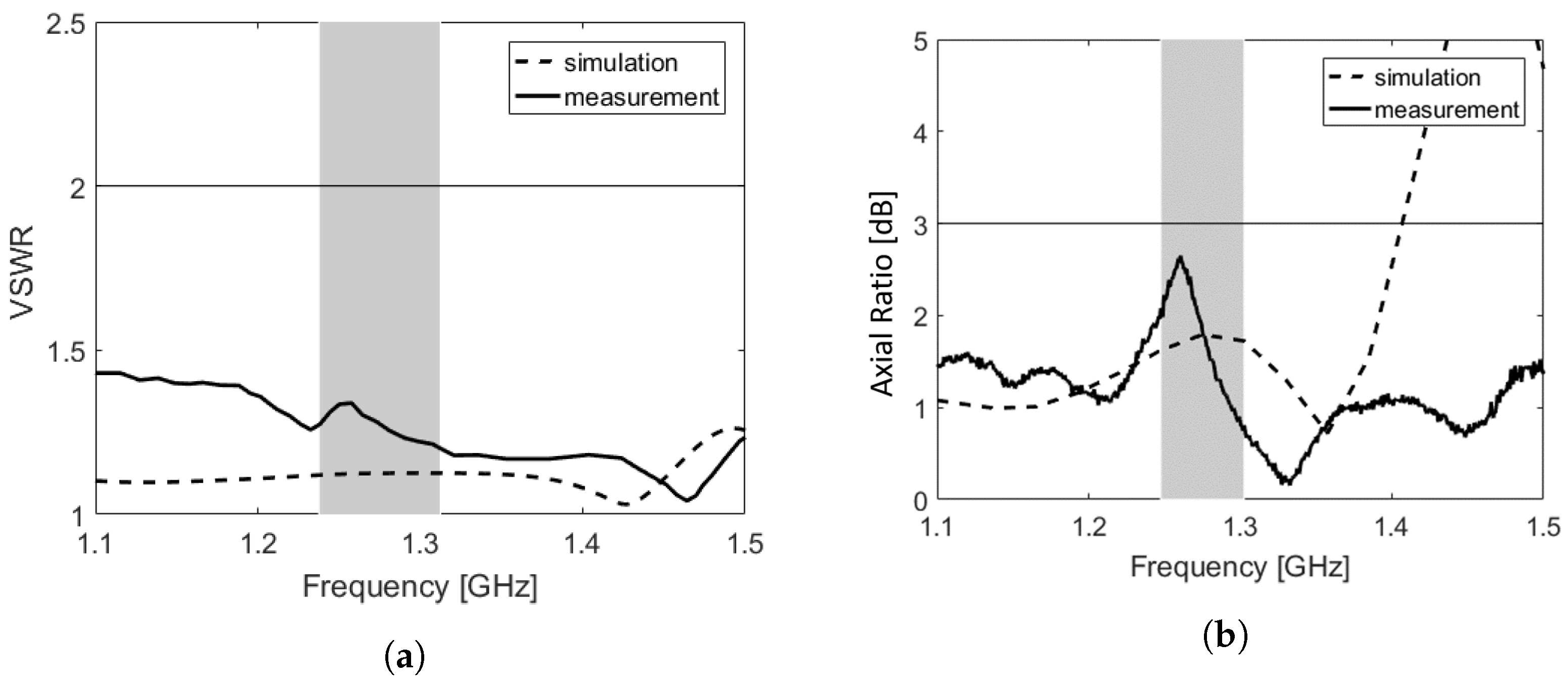
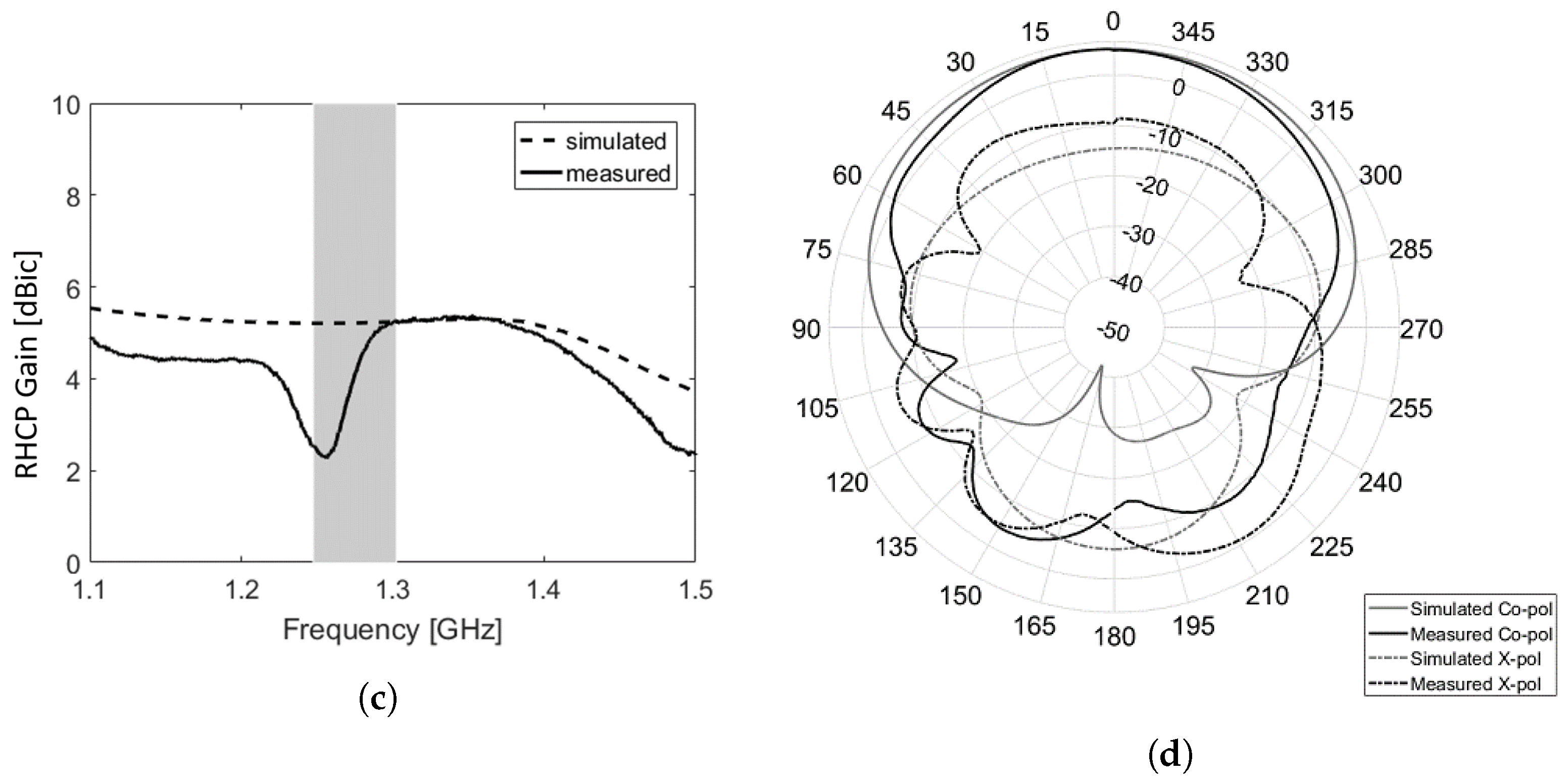
Nf	number of feed turns	0.5

. The antenna pattern was measured in an anechoic chamber using the E8364C PNA Microwave Network Analyzer, and results are depicted in Figure 5 and summarized in

Table 5. Summary of performance of backfire helix at center frequency.

Co-pol (dBic)	HPBW	10dBBW	AR (dB)	X-pol (dBic)	Z ($\mathbf{\Omega }$)
5.7	115.4${}^{\circ }$	157${}^{\circ }$	1.1	−13.1	53-j3.9

.

2.4. Deployment Structure

The stow volume dictated the type of mechanical deployment scheme to be used. The antenna is a wrap-rib type, and the mesh layer is attached to the radial ribs. The ribs are wrapped around the center hub during storage time and at deployment time, as it reverts to its original shape due to the rigidity of the rib. The deployment mechanism steps can be seen in Figure 6a,b. It is a one-time sequence with duration less than 60 s where the antenna unfolds into a deployed state. For this operation, very flexible spring ribs were designed for adequate bending to tolerate tensions until deployment.

Each rib is a parabolic strip cut out from a spring steel plate. To ascertain restoring forces, material properties such as flexibility and rigidity of strip cuts with various configurations were analyzed. Since the rigidity of a single plate is insufficient, making it difficult to wind it around the main hub, a “sandwich” structure is adopted, in which a honeycomb rubber core is disposed between two plates. Therefore, with rubber cores discretely arranged along the ribs, rigidity is improved so that the surface plate can be buckled when bent, so the parabolic shape of the reflector is retained after deployment, guaranteed by the extremely high rigidity of the ribs.

3. Antenna Gain Estimation

The directivity D of a parabolic reflector antenna for a specific frequency is given by ${\left({\displaystyle \frac{\pi d}{\lambda }}\right)}^2$, with d being the reflector diameter, and $\lambda$ the corresponding wavelength, resulting in this case in 33.63 dBic. The gain is then calculated by $G=\eta D$, where $\eta$ is the overall antenna efficiency given by [15], which accounts several factors, such as impedance mismatch, antenna aperture, and reflector surface roughness, among others. These contributions must be estimated for calculating the antenna effective gain. Apart from peak loss, antenna sidelobes must be carefully controlled, as they can increase range ambiguities, degenerating the final image. For the CP-SAR, sidelobe levels must be below $-20$ dBic.

3.1. Perfect Parabolic Reflector

To identify losses introduced by the different elements of the antenna system, the reflector is first optimized for its center frequency, considering a perfect parabolic surface without ribs or feed assembly. A theoretical feed pattern of form $co{s}^n\left(\theta \right)$ was used for the design optimization, with $-10$ dB edge taper. The feed, located at the paraboloid focal point, spreads spherical waves as $\frac{1}{r}$, where r is the distance from the focus to the reflector. These spherical waves are transformed by the paraboloidal reflector into a plane wave propagated to the aperture plane at a constant amplitude.

A theoretical pattern for a circularly polarized feed [16] can be described by

$$E\left(r\right)=A_0{e}^{j\tau \varphi }[\widehat{\theta }{C}_E\left(\theta \right)+\widehat{\varphi }j\tau C_H\left(\theta \right)]\frac{e^{-jkr}}{r}$$

(2)

where $A_0$ is a complex constant, $\tau =+1$ for LHCP or $\tau =-1$ for RHCP, and

$$C_E\left(\theta \right)=C_H\left(\theta \right)={\mathit{cos}}^n\left(\theta \right)$$

(3)

for 0 $<\theta <\frac{\pi }{2}$ in the E- and H-plane patterns, respectively. The parabolic half-angle ${\theta }_0$ is defined as 2$tan\left(\frac{1}{4\frac{f}{D}}\right)=69.39{}^{\circ }$. The variable n relates to the feed illumination taper T in [dB] and ${\theta }_0$, given by:

$$n=\frac{-0.05.T}{log\left[cos\left(\frac{{\theta }_0}{2}\right)\right]}$$

(4)

Ignoring any central blockage, spillover efficiency (${\eta }_{spill}$) and amplitude taper efficiency (${\eta }_{taper}$) are calculated as:

$${\eta }_{spill}=1-u^{2(n+1)}$$

(5)

$${\eta }_{taper}=\frac{4(n+1){(1-u^n)}^2}{n^2[1-u^{2(n+1)}]}{cot}^2\frac{{\theta }_0}{2}$$

(6)

where $u=cos\left({\displaystyle \frac{{\theta }_0}{2}}\right)$.

For an ideal $-10$ dB edge taper feed, amplitude taper and feed illumination efficiency values are ${\eta }_{taper}={\eta }_{spill}=-0.457$ dBic. As for feed blockage losses, they occur around the boresight of the reflector where the field is shadowed by the feed platform. This blocking causes an increase of the SLL due to the discontinuous aperture distribution and the scattering of the incoming wavefront by the blocking structure. Minimizing central blockage requires smaller feed systems. Effect on cross-polarization, axial ratio and sidelobes are studied by modeling a blocking disk with varying radius placed at the parabolic focal point. To keep sidelobe levels below $-25$ dB, maximum dimension of the feed platform has to be no larger than 28.8 cm ($BR=8\%$), with respective ${\eta }_{block}=0.11$ dBic. The backfire helical antenna has a cross-sectional dimension of 8 cm ($BR=2.2\%$), which gives almost negligible blockage losses of 0.002 dBic. On the other hand, the taper and spillover losses sum up to 2.4 dBic for the simulated pattern of the helical antenna. Subtracting ${\eta }_{taper}$, ${\eta }_{spill}$ and ${\eta }_{block}$ from the maximum antenna gain of 33.6 dBic results in peak losses of 1.7 dBic for an ideal parabolic reflector.

3.2. Effect of Ribs

Next, losses regarding the effect of ribs and subsequent quasi-parabolic surface are estimated using the microstrip antenna as feed element. The reflector has supporting ribs that are parabolic in shape and wire mesh stretched between them; that means that the surface between two ribs is a quasi-parabolic area. This gore shape causes phase error loss and their periodicity produces extra sidelobes. Consequently, the focal point of the parabola becomes a spread focal region, within which the feed position has to be optimized [17]. The new feed location that minimizes peak gain loss is at +1.5 cm from the focal point after optimization. Equation (7) calculates the minimum number of gores $N_G$ for a given antenna diameter D, f/D ratio, wavelength $\lambda$, and peak-to-peak phase deviation $\delta$ across the gore. As the number of ribs increases, phase error losses decrease, as the surface becomes closer to a perfect paraboloid. For the current parabolic configuration, using a 10-dB taper feed, at least 11 ribs are needed to keep gore losses below 0.5 dB.

$$N_G=\sqrt{\frac{800-500(\frac{f}{D}-0.4)}{\delta }{\displaystyle \frac{D}{\lambda }}}$$

(7)

When accounting other factors than antenna losses, such as mechanical stability, risk of deployment failure and stowage space, 24 supporting ribs were estimated necessary. After simulating the antenna pattern accounting ribs and gore surface, there was no significant impact on the shape of the main pattern, with peak losses of ${\eta }_{gore}=0.63$ dBic and a slight increase in the sidelobes to $-19.2$ dB.

3.3. Effect of Mesh Reflectivity

The reflector antenna surface is composed of a fine knitted mesh wire of 28 openings per inch (OPI), molybdenum core diameter of 30 $\mathsf{\mu }$m and gold-coated surface of 0.2 $\mathsf{\mu }$m. The small wire diameter together with the excellent RF conditions and softness of the gold plating creates low wire-to-wire contact resistance, which is essential for maintaining good RF performance. The mesh type adopted is woven in a single wire, namely, single atlas pattern. Given that mesh opening size is 325 times smaller than the center wavelength, computer simulation of the mesh parabolic reflector becomes an impossible task. For that reason, transmission loss ${\eta }_t$ of the mesh sample was estimated experimentally by placing a mesh sample between 1 Tx and 1 Rx horn antennas, and measuring the S21 value. Within operational bandwidth, ${\eta }_t=$$-40$ dB. Therefore, the parabolic reflector is assumed solid in antenna simulations, and reflectivity loss is then estimated by direct comparison with measurements of antenna radiation pattern.

3.4. Effect of Struts

Support struts block the aperture of a centrally fed reflector and reduce antenna gain. Because the passing waves induce currents on the struts that radiate, the effect of struts can be larger than their area. The struts have circular cross-section of 10 mm diameter and length of 1.308 m and are illuminated by spherical waves from the feed. Induced currents together with the feed illuminate the reflector. Each strut creates a shadow on the field generated by the feed, which decreases the spillover for $\theta$ larger than zero. A parametric analysis of the effect of number of struts on the radiation pattern is performed, and six main aluminum struts were chosen as they provide good compromise between mechanical stability of the structure and acceptable levels of peak amplitude and SLL for a 10-dB taper feed. Peak losses introduced by the struts were simulated in ${\eta }_{struts}=0.7$ dBic with considerate increase in sidelobe levels of 4 dB and axial ratio increase to 2.2 dB. Although sidelobes are above desired levels, they can be improved in the feed assembly by controlling the distance between elements.

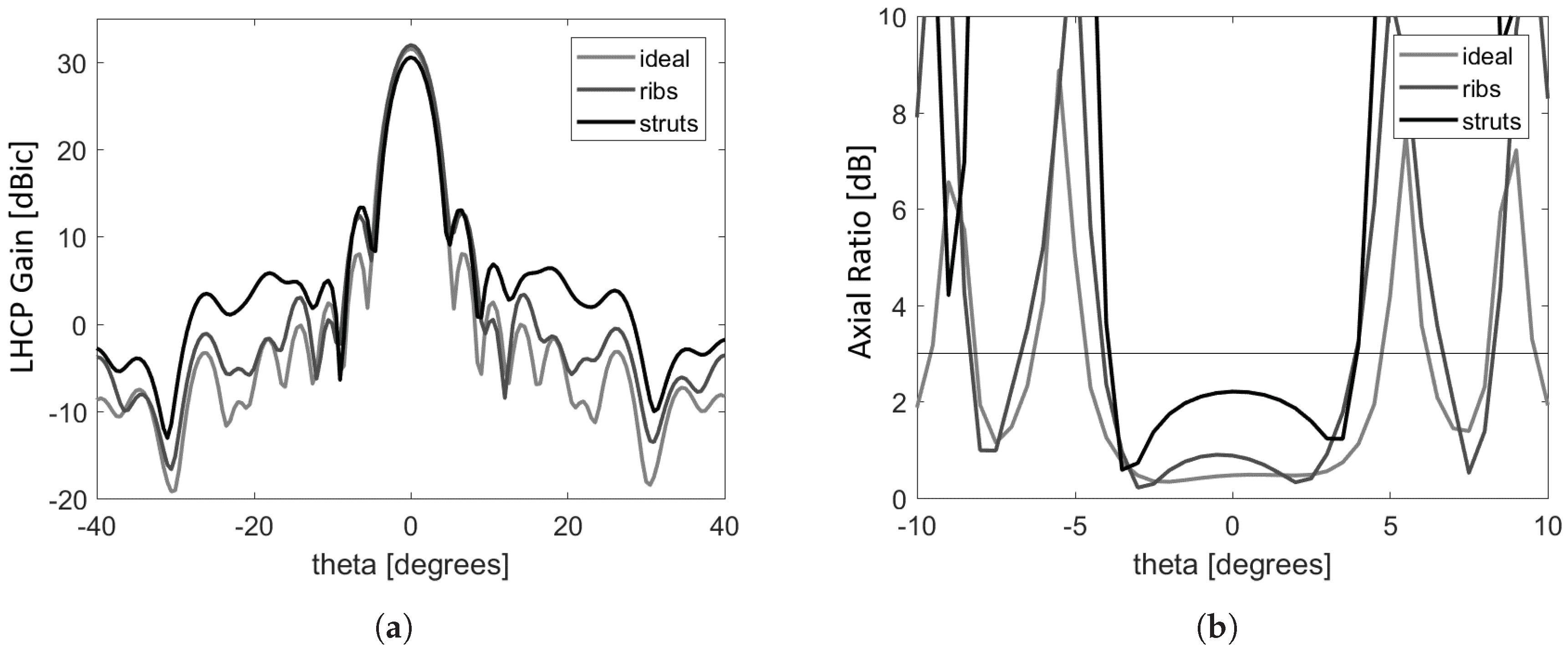
Therefore,

Table 6. Illumination losses at 1.275 GHz: effect of antenna elements on the co-polarized gain (Co-Pol), peak gain losses and peak sidelobe levels (Peak SLL).

Loss Contributions	Co-Pol (dBic)	Peak Loss (dB)	Peak SLL (dB)
Ideal parabolic	33.6	–	–
Spillover, taper, blockage	31.9	1.7	$-27.4$
Mesh	–	0.0027	–
Gore shape	31.3	0.6	$-19.2$
Struts	30.6	0.7	$-15.2$
Total	30.6	3	$-15.2$

and Figure 7a,b summarize these contributions affecting the antenna radiation pattern, with total antenna losses estimated in ${\eta }_{total}=3$ dBic.

4. Validation of Parabolic Mesh Reflector

4.1. Verification of Surface Error

Reflector surface errors, due to fabrication errors, deformations caused by gravity, or roughness of the reflective surfaces, reduce the antenna gain estimated. Antenna surface tolerances were limited to 4.22 mm following Ruze’s prediction for surface tolerance efficiency of 3 dB.

A research model of the deployable parabolic mesh reflector was constructed, as depicted in Figure 8a. Two approaches to measure surface accuracy of the mesh reflector using laser and three-dimensional photogrammetric technique were performed.

4.1.1. Laser Measurements Along Ribs

A reference plane was placed at the bottom of the reflector, and fixed points along the 24 ribs were measured with a laser meter that can be displaced along the reference place. Eleven points distanced 10 cm from each other were marked with reflective tapes. These points were marked on each rib’s lateral, i.e., along its right and left sides. Misalignment errors were included in overall surface error. RMS surface error was computed as the RMS difference between theoretical value of parabolic rib shape and measured values. Results show average RMS error of 1.92 mm ± 1.125 mm on the right side of the rib and 1.93 mm ± 0.53 mm on the left side of the rib, both below the required 4.22 mm RMS surface error.

4.1.2. 3D Scanning of Mesh Reflector Surface

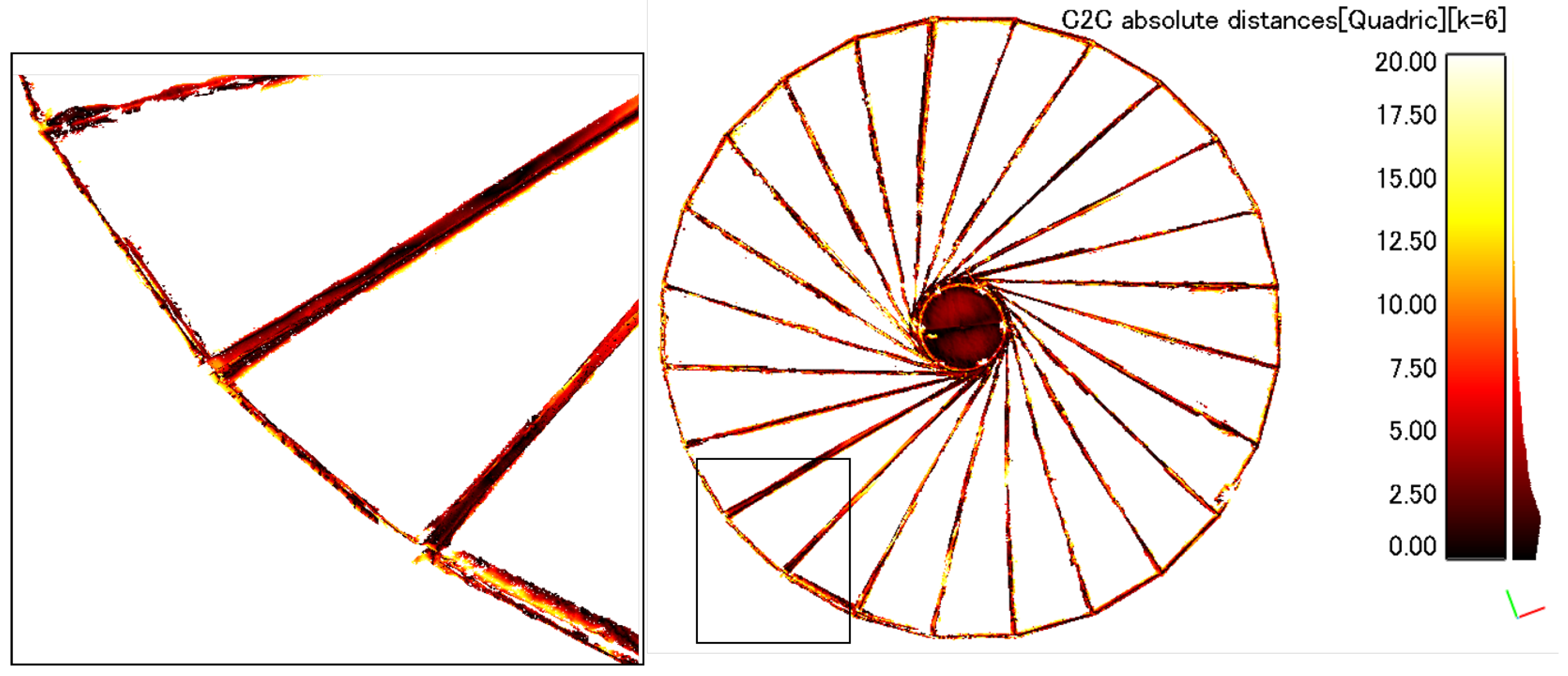
To scan the reflector surface, the photogrammetric device was placed 2 m away from the center of parabolic reflector. A commercial 3D scanning device was used for reflector contour measurement [18]. Eleven overlapping images composed of triangular mesh cells were generated, covering the reflector surface area with spatial resolution of 1 mm. To avoid background scattering from the surroundings, an anti-reflective sheet was placed behind the reflector. The measurements showed that, although detectable, the thin mesh material scatters the projected light more than it reflects back towards the camera, resulting in very noisy surface estimations. Since the ribs presented clear shape, they were then used as measured reference for reflector shape. Each scan then was converted into a point cloud of 2,500,000 points. Noise and artifacts were removed and filtered. Each point cloud scan was then directly compared with the theoretical parabolic surface using a best fit function, and these distances computed as errors. Cloud-to-cloud (C2C) distances computations were based on a quadratic function. A surface map of calculated C2C distances using the k-nearest neighbor classifier can be seen in the color map displayed in Figure 9. Standard deviation $std$ and mean $\mathsf{\mu }$ of the normal distribution of C2C distances were computed, with overall RMS error of 3.86 mm.

4.2. Near-Field Antenna Measurements

Antenna pattern measurements were realized with a near-field plane polar system at A-METLAB facilities at Kyoto University, composed of a robot scanner, a dual-linearized probe, and a computer subsystem. The helical antenna was placed at position z = $-2$ cm, considering the parabolic and helical antenna’s phase center. Measurements were realized in the frequency range of 1.1–1.55 GHz. From the sampled radiating near-field, the data could be later converted into far-field. The measuring probe was located in the ceiling, and the antenna under test (AUT) on a lifting table over a turn plane on the ground. Figure 8b illustrates the planar near-field measurement system setup. The distance from probe to AUT was 1.1 m. The probe gathered 57 points within a radius of 2.7 m at 0.09 m spacing, and 91 points on a polar fashion at 2${}^{\circ }$ step. Far-field points were derived, 201 points in the azimuth and elevation directions, ranging from $-{60}^{\circ }$ to +60${}^{\circ }$, at step angle of 0.6${}^{\circ }$. 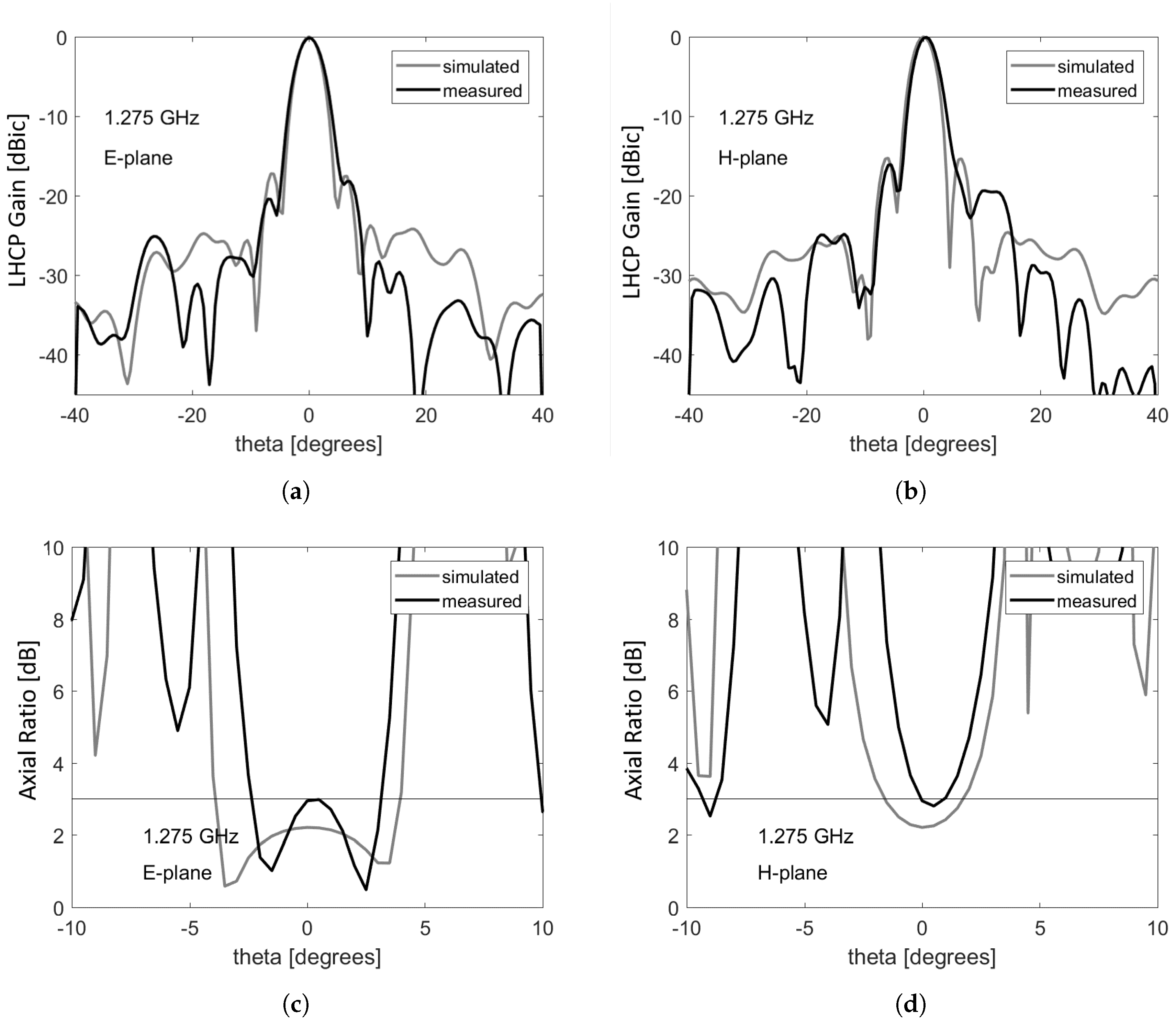Results are depicted in Figure 10, showing simulated and measured far-field antenna directivity at center frequency. Directivity measured was 29.86 dB, with peak slightly deviated from the boresight by 0.38${}^{\circ }$. Highest measured SLL was 15.8 dB, and axial ratio 2.94 dB at center frequency. A summary of simulated and measured results are in

Table 7. Summary of results of near-field antenna measurements at minimum, center, and maximum frequencies ($f_{min}$, $f_c$, $f_{max}$) regarding: peak co-polarization at boresight (Co-pol), axial ratio (AR) at boresight, half-power beam width (HPBW), sidelobe levels (SLL) and cross-polarization at boresight (Cross-pol).

	Co-pol (dBic)	AR (dB)	HPBW	SLL (dB)	Cross-pol (dBic)
Measured at $f_{min}$	29.8	2.25	4.2${}^{\circ }$	$-16.86$	12.9
Measured at $f_c$	29.84	2.94	3.8${}^{\circ }$	$-15.86$	12.8
Measured at $f_{max}$	29.7	2.37	4.1${}^{\circ }$	$-15.2$	13.8
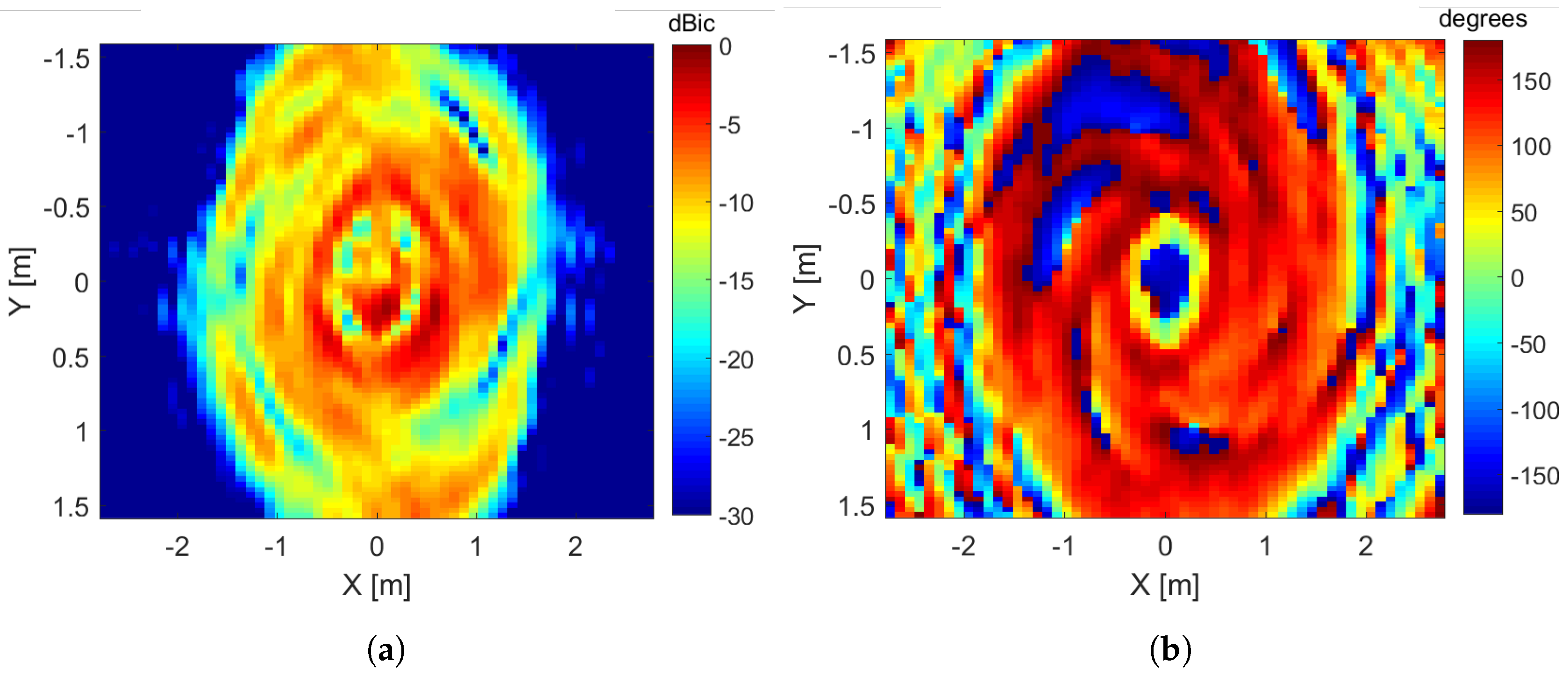
Simulated at $f_c$	30.6	2.2	4${}^{\circ }$	$-15.2$	24.4

for minimum, center and maximum frequencies. From the near-field measurements, holographic maps were also derived, displaying amplitude and phase data of co-polarization field in center frequency in Figure 11.

5. Discussion

Since the mesh material is fixed on the reflector structure by being stretched and stitched around ribs and rims, there is an added volume of mesh material over these structures. Hence, in both measurement methods for geometric surface verification, some deviation from the theoretical model is expected. Additionally, the reflector position in each measurement setup was different; in the laser measurement, the reflector was facing upwards, whereas in the 3D scanning measurement setup, it was facing almost horizontally. Therefore, reflector surface distortions due to gravity are also expected to be different in each measurement setup. Results from the laser measurements presented largest discrepancy from rib number 9, with 3.6 mm RMS, and overall ribs measurements presented 1.92 mm RMS, lower than the required surface accuracy of 4.22 mm RMS.

The 3D scanning results, on the other hand, presented higher RMS error of 3.86 mm. This difference in surface accuracy error can be attributed to the low image SNR of mesh material when 3D scanned, possible image misregistration of scanned patches, and more significant reflector distortion due to gravity compared to the laser setup. In the future, errors in the image processing steps can be reduced by using geo-referenced reflective tags on the parabolic surface under the same 3D scanning approach.

Results from the near-field antenna pattern measurement showed good agreement between simulation and measured data in both azimuth and elevation planes. The overall antenna gain can be improved by increasing the helical feed gain to comply with the required 30 dBic. That can be simply done by increasing the number of helical loops. Measured axial ratio also reasonably agreed with simulations, but showed considerable axial ratio degeneration of 0.7 dB when compared to simulated results. This together with other small deviations could be attributed to unavoidable misalignment in the setup between the helical antenna and center of parabolic reflector, as well as effects of the mesh weaver pattern in the circularly polarized wave.

Some degeneration of simulated versus measured values of axial ratio, co- and cross-polarization can be seen at boresight, as referred in Table 7 and Figure 10. These differences can be attributed to unavoidable misalignments in the setup, as well as effects of the knitted mesh pattern for circularly polarized waves, since, in the simulations, the reflector was assumed rigid. Adopting a mesh type with a pair of wires instead of single wire can reduce the variance of reflectivity dependant on the direction of electric field of the incident wave, as previously reported for 20 GHz frequencies [19]. Hence, further investigations on the mesh reflectivity for CP waves in the L-band must be carried out. Moreover, measured sidelobe levels presented good agreement with simulation results, but still present higher values than the specification. Further adaptation of feed tower must be carried out to minimize cross-polarization and sidelobe values.

Figure 11a is a holographic amplitude map at the antenna aperture, which can be interpreted as the illumination efficiency of feed on the main reflector. A near 10-dB taper feed can be seen, as expected from measured and simulated helical antenna patterns. Additionally, the amplitude map shows few areas with uneven illumination. That can be explained by a series of factors: diffraction due to struts and other elements, an improperly focused antenna, reflector surface distortions and potential misalignment in the setup. Precise alignment between probe and reflector platform was not possible due to unavoidable vibrations from the lifting table, which could have resulted in slight movements of the antenna configuration.

The holographic phase map gives a good approximation of surface distortions, and jumpy phases of ±180${}^{\circ }$ can be seen as the phase is still wrapped. Although the generated phase hologram is not focused over the reflector surface at all points, it still gives an idea of surface errors, showing that no large surface distortions can be observed as the phase looks uniform within reflector area.

Validation of the deployable mesh parabolic reflector presented overall good results, but further analysis on the strut design must be conducted to minimize scattering effects. Additionally, future work should focus on the development of the feed assembly for a full polarimetric configuration, and later tested with the reflector.

6. Conclusions

This paper describes the design and development status of a compact CP-SAR system compatible with a 150-kg class satellite. Small satellites introduce a new realm of options for their low costs and reduced manufacturing time of the spacecraft platforms, becoming very attractive alternatives to traditional remote sensing missions. The L-band CP-SAR microsat is a technology demonstrator and compact science mission for disaster mitigation using L-band CP-SAR developed by Chiba University and LAPAN. The key technology for a compact design is mainly based on the SAR antenna; the antenna is of deployable type, with total mass less than 15 kg and carefully designed to fit piggy-back volume and weight constraints. The deployable reflector is a center-fed parabolic mesh with diameter of 3.6 m.

In this work, mission specification and overall design parameters are presented, justifying the use of the deployable mesh parabolic reflector in the current mission. Simulation and measurements of antenna radiation are presented, with contributions of different antenna elements to the final radiation pattern. Antenna surface estimation was realized using a laser distance meter along ribs and scanning the reflector surface with a 3D scanning device, resulting in surface accuracy values of 1.92 mm and 3.86 mm RMS, below the required 4.22 mm. Near-field antenna measurements also confirmed good agreement with simulated results of the parabolic mesh reflector with a backfire helix antenna as feed. Few parameters must be improved to comply with mission specifications: peak directivity, by increasing the number of loops of the helical antenna, and sidelobe levels, by modifying the current tower struts design to reduce the scatterings.

Additional future work should concentrate in prototyping/testing the feed assembly, and further investigations on improving the overall antenna efficiency.

References

- Gao, S.; Clark, K.; Unwin, M.; Zackrisson, J.; Shiroma, W.A.; Akagi, J.M.; Maynard, K.; Garner, P.; Boccia, L.; Amendola, G.; et al. Antennas for Modern Small Satellites. IEEE Antennas Propag. Mag. 2009, 51, 40–56. [Google Scholar] [CrossRef]
- Ouchi, K. Recent Trend and Advance of Synthetic Aperture Radar with Selected Topics. Remote Sens. 2013, 5, 716–807. [Google Scholar] [CrossRef]
- Naftaly, U.; Levy-Nathansohn, R. Overview of the TECSAR Satellite Hardware and Mosaic Mode. IEEE Geosci. Remote Sens. Lett. 2008, 5, 423–426. [Google Scholar] [CrossRef]
- Korczyk, J. Reliable on Board Data Processing System for the ICEYE-1 Satellite. Master’s Thesis, KTH, School of Information and Communication Technology (ICT), Stockholm, Sweden, 2016. [Google Scholar]
- Hodges, R.E.; Radway, M.J.; Toorian, A.; Hoppe, D.J.; Shah, B.; Kalman, A.E. ISARA—Integrated Solar Array and Reflectarray CubeSat deployable Ka-band antenna. In Proceedings of the 2015 IEEE International Symposium on Antennas and Propagation USNC/URSI National Radio Science Meeting, Vancouver, BC, Canada, 19–24 July 2015; pp. 2141–2142. [Google Scholar]
- Motohka, T.; Kankaku, Y.; Suzuki, S. Advanced Land Observing Satellite-2 (ALOS-2) and its follow-on L-band SAR mission. In Proceedings of the 2017 IEEE Radar Conference (RadarConf), Seattle, WA, USA, 8–12 May 2017; pp. 953–956. [Google Scholar]
- Mobrem, M.; Kuehn, S.; Spier, C.; Slimko, E. Design and performance of Astromesh reflector onboard Soil Moisture Active Passive spacecraft. In Proceedings of the 2012 IEEE Aerospace Conference, Big Sky, MT, USA, 3–10 March 2012; pp. 1–10. [Google Scholar]
- Thomson, M.W. The AstroMesh deployable reflector. In Proceedings of the IEEE Antennas and Propagation Society International Symposium. Held in Conjunction with: USNC/URSI National Radio Science Meeting (Cat. No. 99CH37010), Orlando, FL, USA, 11–16 July 1999; Volume 3, pp. 1516–1519. [Google Scholar]
- Akbar, P.R.; Tetuko, S.S.J.; Kuze, H. A novel circularly polarized synthetic aperture radar (CP-SAR) system onboard a spaceborne platform. Int. J. Remote Sens. 2010, 31, 1053–1060. [Google Scholar] [CrossRef]
- Raney, R.K. Hybrid-Quad-Pol SAR. In Proceedings of the IGARSS 2008—2008 IEEE International Geoscience and Remote Sensing Symposium, Boston, MA, USA, 7–11 July 2008; Volume 4, pp. IV-491–IV-493. [Google Scholar]
- Izumi, Y.; Demirci, S.; Baharuddin, Z.; Sri Sumantyo, J.; Yang, H. Analysis of circular polarization backscattering and target decomposition using GB-SAR. Prog. Electromagn. Res. B 2017, 73, 17–29. [Google Scholar] [CrossRef]
- Llop, J.; Roberts, P.; Hao, Z.; Tomas, L.; Beauplet, V. Very Low Earth Orbit mission concepts for Earth Observation: Benefits and challenges. In Proceedings of the Reinventing Space Conference, London, UK, 18–20 November 2014. [Google Scholar]
- CST—Computer Simulation Technology GmbH. Available online: https://www.cst.com/products/csts2 (accessed on 17 December 2018).
- Nakano, H.; Yamauchi, J.; Mimaki, H. Backfire radiation from a monofilar helix with a small ground plane. IEEE Trans. Antennas Propag. 1988, 36, 1359–1364. [Google Scholar] [CrossRef]
- Kildal, P. Factorization of the feed efficiency of paraboloids and Cassegrain antennas. IEEE Trans. Antennas Propag. 1985, 33, 903–908. [Google Scholar] [CrossRef]
- Sharma, S.K.; Rao, S.; Shafai, L. Handbook of Reflector Antennas and Feed Systems: V.1 Theory and Design of Reflectors; Artech House: Norwood, MA, USA, 2013. [Google Scholar]
- Ingerson, P.; Wong, W. The analysis of deployable umbrella parabolic reflectors. In Proceedings of the 1970 Antennas and Propagation Society International Symposium, Ohio State University, OH, USA, 14–16 September 1970; Volume 8, pp. 18–20. [Google Scholar]
- DAVID Vision Systems. Available online: https://www.david-3d.com/en/support/david4/introduction (accessed on 17 December 2018).
- Miura, A.; Tanaka, M. A mesh reflecting surface with electrical characteristics independent on direction of electric field of incident wave. In Proceedings of the IEEE Antennas and Propagation Society Symposium, Monterey, CA, USA, 20–25 June 2004; Volume 1, pp. 33–36. [Google Scholar]
Figure 1.
Trends in miniaturization of past, current and future spaceborne SAR missions: spacecraft mass versus range resolution for dB.
Figure 2.
Dependency of usable PRFs (white area) as incidence angles vary. Unavailable PRF values due to blind ranges and nadir returns are depicted in yellow and blue.
Figure 3.
Deployable parabolic reflector in (a) profile and (b) top view.
Figure 4.
(a) Side and top view of backfire helix antenna; and (b) constructed helix and wavetrap used for impedance matching.
Figure 5.
Simulation and measurement results of backfire helical antenna within operational bandwidth: (a) VSWR; (b) axial ratio; (c) directivity in co-polarization; and (d) polar plot of co- and cross-polarization at E-plane center frequency.
Figure 6.
Conceptual mechanism of wrap-rib deployment and deployment test of wrap-rib reflector.
Figure 7.
Simulated antenna pattern radiation accounting different elements contribution at center frequency: (a) co-polarized gain, and (b) axial ratio.
Figure 8.
(a) Research model of deployable parabolic mesh reflector antenna; and (b) near-field measurement setup.
Figure 9.
Computed cloud-to-cloud (C2C) absolute distances in millimetres between reflector model and scanned areas of reflector ribs, rims and center plate.
Figure 10.
Simulation and measurement results at center frequency of RHCP directivity in the: (a) E-plane; (b) H-plane; and axial ratio in the: (c) E-plane; and (d) H-plane.
Figure 11.
Hologram at aperture level in center frequency of: (a) field amplitude; and (b) phase.