Deep Q-Network for Maneuver Planning in Beyond-Visual-Range Aerial Pursuit–Evasion with Target Re-Engagement

Abstract

Decision-making for maneuvering in the presence of long-range threats is crucial for enhancing the safety and reliability of autonomous aerial platforms operating in beyond-line-of-sight environments. This study employs the Deep Q-Network (DQN) method to investigate maneuvering strategies for simultaneously avoiding incoming high-speed threats and re-establishing tracking of a maneuvering target platform. First, kinematic models for the aerial platforms and the approaching interceptor are developed, and a DQN training environment is constructed based on these models. A DQN framework is then designed, integrating scenario-specific state representation, action space, and a hybrid reward structure to enable autonomous strategy learning without prior expert knowledge. The agent is trained within this environment to achieve near-optimal maneuvering decisions, with comparative evaluations against Q-learning and deep deterministic policy gradient (DDPG) baselines. Simulation results demonstrate that the trained model outperforms the baselines on key metrics by effectively avoiding approaching threats, re-establishing robust target tracking, reducing maneuver time, and exhibiting strong generalization across challenging scenarios. This work advances Beyond-Visual-Range (BVR) maneuver planning and provides a foundational methodological framework for future research on complex multi-stage aerial pursuit–evasion problems.

1. Introduction

Beyond-Visual-Range (BVR) aerial engagements refer to scenarios where two aircraft detect each other using onboard sensors and interact in the presence of medium-to-long-range interceptor threats [1]. Achieving favorable performance during the BVR phase typically requires satisfying two conditions: (1) employing strategic maneuvers within load-factor limits to avoid incoming threat trajectories and enhance platform safety; and (2) performing advantageous maneuvers that account for radar coverage and propulsion characteristics to maintain effective sensing range and achieve robust target tracking. With the rapid development of onboard equipment and long-range interceptor technology, modern high-overload, high-speed threat vehicles have substantially increased the proportion of interactions that conclude during the BVR phase. Therefore, devising intelligent maneuvering strategies within platform maneuverability limits to avoid approaching threats and re-establish target tracking after avoidance is crucial for improving safety and overall mission effectiveness in BVR scenarios [2].

Among the most cost-effective and efficient methods for avoiding dynamic aerial obstacles, both domestic and international scholars have extensively studied optimal or suboptimal maneuvering strategies for aircraft obstacle avoidance. Traditional threat-avoidance strategies primarily employ expert systems [3,4,5,6], differential game theory [7,8,9,10], and optimal control methods [11,12,13,14]. However, expert systems are highly dependent on human expertise, complex to encode, and lack generalizability [15]. Differential game theory and optimal control methods require precise mathematical models, involve complex calculations, and are difficult to solve [16]. These methods are limited in their applicability to BVR aerial maneuvering research, due to the inherent complexity of such operational scenarios.

As artificial intelligence continues to advance, the integration of reinforcement learning and deep neural networks has formed a direct control algorithm that does not require modeling. This end-to-end learning approach enables the transition from raw input to output [17], has been extensively utilized across various aerial engagement research areas over the past few years [18]. Wang et al. [19] proposed an autonomous attack decision-making method based on hierarchical virtual bayesian reinforcement learning. Recognizing the limitations of traditional reinforcement learning and DQN algorithms in handling continuous action spaces, they proposed an improved DDPG algorithm to enhance learning efficiency. Keong et al. [20] formulate the collision avoidance process as a Markov Decision Process (MDP) and investigated the performance of DQN in aerial collision avoidance. However, these studies primarily focus on Within-Visual-Range aerial engagement and are not well-suited for the more complex BVR aerial engagement scenarios.

For threat-avoidance maneuver decision-making, Fan et al. [21] employed a simplified aircraft model and the DDPG algorithm to train evasion maneuver decision-making methods. They conducted simulation verification of the effectiveness of evasion maneuvers in four typical initial scenarios, but the study involved a simplified model and a limited range of initial scenarios, failing to validate the effectiveness of the learned evasion strategies. Although the DDPG algorithm studies have advantages in handling continuous action spaces, they target relatively simple task scenarios and suffer from slow convergence and susceptibility to local optima, making them unsuitable for more complex scenarios involving post-evasion target re-engagement. Wang et al. [22] performed a comparison of DQN and DDPG in autonomous maneuver decision-making for aircraft, concluding that DQN exhibits better decision-making capabilities under the same task complexity. Özbek et al. [23] proposed a deep reinforcement learning approach for generating online interceptor-evading maneuvers for aerial vehicles. The system employs Twin Delayed Deep Deterministic Policy Gradient (TD3), one of the most known deep reinforcement learning algorithms, to train an agent to make real-time decisions on the best evasion tactics in a complex environment.

However, the aforementioned studies only address threat avoidance in BVR aerial engagements. The maneuvers learned through deep reinforcement learning algorithms typically involve large turns that place the interceptor behind the platform but also cause the agent aircraft to turn away from the target. As a result, the onboard radar may fail to maintain or re-establish tracking after the avoidance phase, leaving the agent in an unfavorable sensing configuration.

Although reinforcement learning has advanced autonomous decision-making in aerial maneuvering, most existing studies focus on single-phase avoidance, overlooking subsequent target re-acquisition. This gap limits the completeness of multi-stage Beyond-Visual-Range (BVR) engagement scenarios, where both threat avoidance and subsequent target tracking are important.

To address these issues, this paper constructs a training framework for BVR maneuver decision-making using DQN. We define the BVR task scenario as follows: In a 1 vs. 1 BVR aerial engagement, the agent aircraft and a target aircraft are flying head-on. When facing an approaching interceptor launched toward the agent, the agent performs evasive maneuvers to avoid the threat while simultaneously re-establishing tracking of the target aircraft, preparing for subsequent interaction. The research involves scenario modeling, algorithm adaptation, and multi-configuration testing to validate strategy rationality and generalization. The main contributions of this paper are summarized as follows.

(1)

A model-free DQN-based deep reinforcement learning approach is employed for autonomous maneuver decision-making, distinct from traditional methods like expert systems or optimal control. This innovation eliminates reliance on handcrafted rules or precise system modeling, improving adaptability to complex dynamic aerial adversarial environments and reducing manual engineering overhead.

(2)

A DQN framework tailored for discrete-action maneuver planning in BVR scenarios is proposed, differing from prior studies using DDPG or A2C (methods suited for continuous action spaces but prone to slow convergence and local optima). Scenario-specific state representation and action space design enable more stable training and superior decision performance in BVR-characteristic discrete maneuver tasks.

(3)

A hybrid reward structure integrating sparse terminal and dense process-based rewards is designed to accelerate learning and enhance policy effectiveness in realistic interceptor evasion and target reacquisition. The trained agent’s generalization capability is validated across challenging test scenarios, exhibiting robust decision-making independent of prior knowledge.

The remainder of this paper is organized as follows. Section 2 details the development of the aerial engagement simulation environment. Section 3 presents the DQN algorithm formulation, its network architecture, and the corresponding implementation workflow. Section 4 describes the simulation experiments, including distinct test scenarios from the training phase, and analyzes the obtained results. Section 5 provides a discussion of the DQN’s performance advantages, real-world implications, and potential limitations. Finally, Section 6 summarizes the work and draws conclusions.

2. Aerial Engagement Environment Design

In this section, we establish the fundamental model for 1 vs. 1 BVR aerial engagement, including kinematic and dynamic models for aircraft and interceptors, onboard radar model and guidance and control system model, and we have also provided the termination conditions for the constructed combat model.

2.1. Model Assumptions and Limitations

To simplify the BVR Aerial Engagement problem and improve computational efficiency, several assumptions are made:

(1)

side-slip and wind effects are neglected;

(2)

the aircraft is assumed to be in torque balance during maneuvers;

(3)

both aircraft and interceptor are modeled as maneuverable point masses; and

(4)

radar lock is idealized without sensor noise or jamming.

These assumptions, commonly used in BVR simulations, provide modeling simplicity but ignore aerodynamic coupling, atmospheric disturbances, and radar uncertainty, which will be addressed in future high-fidelity modeling.

2.2. Kinematic and Dynamic Models for Aircraft and Dynamic Aerial Obstacles

Based on the modeling assumptions described in Section 2.1, the aircraft and interceptor model adopts a maneuverable point-mass model. Key parameters and the kinematic/dynamic formulation used in this study follow Imado et al. [24], supplemented by [25,26]. These idealized assumptions, widely used in BVR aerial-engagement simulation for their simplicity and computational efficiency, form the basis of the dynamic models in this study.

Based on the aforementioned assumptions and fundamental principles of flight mechanics, the dynamics equations of motion for the aircraft in trajectory coordinates can be expressed as follows:

$$\begin{array}{c}\hfill \begin{array}{c}\hfill \left\{\begin{array}{c}{\dot{v}}_i={\displaystyle \frac{T_i-D_i}{m_i}}-gsin{\theta }_i=g(n_{ix}-sin{\theta }_i)\hfill \\ {\dot{\theta }}_i={\displaystyle \frac{g}{v_i}}(n_{in}cos{\varphi }_i-cos{\theta }_i)={\displaystyle \frac{g}{v_i}}(n_{iz}-cos{\theta }_i)\hfill \\ {\dot{\psi }}_i={\displaystyle \frac{g{n}_{in}sin{\varphi }_i}{v_{i}cos{\theta }_i}}={\displaystyle \frac{g{n}_{iy}}{v_{i}cos{\theta }_i}}\hfill \end{array}\right.\end{array},\end{array}$$

(1)

where $i=m,t$ represent interceptor and aircraft, respectively. T represents the thrust of the aircraft, D represents aerodynamic drag, v denotes flight speed, and $\psi$, $\theta$, $\varphi$ respectively represent the yaw, pitch, and roll angles of the aircraft and interceptor. Variables $n_{ix}$ and $n_{in}$ represent the tangential and normal overloads respectively, while $n_{iy}$ and $n_{iz}$ denote the two components of the normal overload along the y-axis and z-axis. Therefore, under the point-mass model assumptions established in this paper, the control variables for the interceptor are $n_{iy}$ and $n_{iz}$, and for the aircraft are $n_{ix}$, $n_{in}$ and ${\varphi }_t$.

The kinematic equation for the aircraft’s center of mass is [25]:

$$\begin{array}{c}\hfill \begin{array}{c}\hfill \left\{\begin{array}{c}{\dot{x}}_i=v_{i}cos{\theta }_{i}cos{\psi }_i\hfill \\ {\dot{y}}_i=v_{i}cos{\theta }_{i}sin{\psi }_i\hfill \\ {\dot{z}}_i=v_{i}sin{\theta }_i\hfill \end{array}\right.\end{array},\end{array}$$

(2)

where $x_i$, $y_i$ and $z_i$ denote the three-dimensional coordinates of the aircraft center in the ground coordinate system, respectively.

2.3. Onboard Radar Model

Once activated, the onboard radar conducts a wide-area search scan to detect targets. Upon detecting and successfully locking onto a target, the onboard radar provides more precise target information to the aircraft, enabling tracking of the target. Research on onboard radar systems is currently quite advanced. For the purposes of this study scenario, we assume that if a target remains within the radar range for more than 1 s, it can be considered successfully locked onto. The radar range of the agent aircraft is detailed in Table 1.

Table 1. The range of the onboard radar.

Symbol	Range	Description
$ES{M}_{{\psi }_e}$	$[-60°,60°]$	Horizontal azimuth angle of the target with respect to the agent aircraft
$ES{M}_{{\theta }_e}$	$[-30°,30°]$	Vertical elevation angle of the target with respect to the agent aircraft

2.4. Guidance and Control System Model

The relative motion module requires input of the position vectors of both the aircraft and the interceptor. In actual aerial combat scenarios, to enable the interceptor to continuously track its target, interceptors are equipped with guidance systems designed to acquire the aircraft’s position, thereby establishing the target line of sight. The guidance system initiates its mission by first searching for targets within radar detection range. Upon successful acquisition, it switches to tracking mode and continuously computes the angular velocities of pitch and yaw lines of sight. In this paper, in deriving and solving the relative motion between aircraft and interceptor, a simplified kinematic guidance system is employed, neglecting errors in the interceptor’s line of sight during the settlement process.

Figure 1 shows an inertial coordinate system that is established with the interceptor’s position as its origin. ${\theta }_L$ is the angle between the $O{X}_g{Y}_g$ plane and the line connecting the aircraft and the interceptor. On the other hand, ${\psi }_L$ is defined as the angle between the $O{Y}_g$ axis and the projection of this line onto the $O{X}_g{Y}_g$ plane. Therefore, the scalar equation for the separation between the aircraft and the interceptor is [27]:

$$\begin{array}{c}\hfill \begin{array}{c}\hfill \left\{\begin{array}{c}{r}_x=x_t-x_m\hfill \\ r_y=y_t-y_m\hfill \\ r_z=z_t-z_m\hfill \\ r=\sqrt{r_x^2+r_y^2+r_z^2}\hfill \end{array}\right.\end{array}.\end{array}$$

(3)

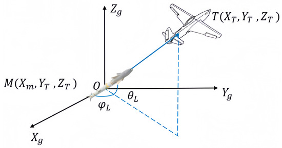
Figure 1. Relative motion model.

Therefore, the pitch angle velocity and yaw angle velocity can be expressed as:

$$\begin{array}{c}\hfill \begin{array}{c}\hfill \left\{\begin{array}{c}{\dot{\theta }}_L=(r{\dot{r}}_z-r_z\dot{r})/r\sqrt{r_x^2+r_y^2}\hfill \\ {\dot{\psi }}_L=(r_x{\dot{r}}_y-r_y{\dot{r}}_x)/r\sqrt{r_x^2+r_y^2}\hfill \end{array}\right.\end{array}.\end{array}$$

(4)

The most mature guidance method currently used in engineering applications is proportional guidance. Considering the kinematic and dynamic models (as Equations (1) and (2)), the normal overload control signal for the interceptor is given as follows:

$$\begin{array}{c}\hfill \begin{array}{c}\hfill \left\{\begin{array}{c}{n}_{my}=(v_{m}K{\dot{\psi }}_{L}cos{\theta }_m)/g\hfill \\ n_{mz}=v_{m}K{\dot{\theta }}_L/g+cos{\theta }_m\hfill \end{array}\right.\end{array},\end{array}$$

(5)

where K is the proportional guidance coefficient.

2.5. Termination Conditions for the Aerial Engagement

Based on the established kinematic models of aircraft and interceptors, as well as the guidance control models, it is possible to construct the entire combat sequence for a 1 vs. 1 BVR aerial engagement scenario. Table 2 outlines the termination conditions for the established simulation environment.

Table 2. Termination conditions.

Termination Symbol	Definition	Satisfied Conditions	Engagement Result
1	aircraft speed	$v_t<180$ m/s or $v_t>600$ m/s	Aircraft stall
2	aircraft altitude	$h_t<500$ m or $h_t>15,000$ m	Aircraft collision or engine failure
3	interceptor speed	$v_m<200$ m/s	interceptor stall
4	interceptor altitude	$h_m<500$ m or $h_m>15,000$ m	Interceptor stall
5	Maximum duration of engagement	$t_1=90$ s	Reaching maximum engagement time
6	relative distance	$r<200$ m	Threat avoidance failed
7	The onboard radar detected the target aircraft within its range for 1 s	$|ES{M}_{{\psi }_e}| < 60°$ and $|ES{M}_{{\theta }_e}| < 30°$ and $t=1$ s	Successful target reacquisition

3. Aerial Engagement Model with Reinforcement Learning

3.1. Reinforcement Learning

Reinforcement Learning (RL) is a machine learning approach that learns to take actions by interacting with the environment, aiming to maximize cumulative rewards [17]. Its core concept involves continuously improving the policy through trial and error, ultimately discovering the optimal policy to solve the problem. A common RL framework is depicted in Figure 2, which can be described as a four-tuple: $⟨S,A,P,R⟩$. S is the state set, which represents the collection of all possible states in the environment; the action set A represents all possible actions that the agent can execute in each state. At each time step, the agent selects an action to execute based on the current state. The state transition probability P represents the probability distribution for moving from one state to another.

Figure 2. Reinforcement learning framework.

The reward function $R(s,a,s^{\prime })$ represents the reward earned by moving from state s to state $s^{\prime }$ after performing action a. In an RL model, the maximum cumulative reward can be achieved by computing the optimal value functions, which yield the optimal values for each state. These values are then utilized to identify the policy that achieves the highest possible cumulative reward.

DQN [28] is an algorithm suitable for solving tasks with discrete action spaces. This algorithm uses neural networks to approximate the state-action value function, overcoming the limitations of traditional RL methods that struggle with large state and action spaces using conventional storage techniques. Additionally, DQN employs batch training, which allows it to cover a larger state space and achieve more stable training results.

3.2. DQN Framework for BVR Maneuver Decision-Making

In this section, we present the 1 vs. 1 BVR maneuver decision-making framework using DQN [28], as depicted in Figure 3. The framework encompasses two primary functions: (a) Developing the agent model based on the aerial engagement environment design outlined in Section 2. (b) Creating the data interface for the reinforcement learning environment to facilitate interactions between the agent and the environment.

Figure 3. DQN BVR maneuver decision-making framework.

The agent primarily functions as the agent aircraft under the interceptor lock-on. Based on the current state, it maps the aerial engagement situation to maneuver control commands. The RL training environment comprises several modules, including the state transition function, reward function, and termination conditions. The training and application of the agent are conducted on an episodic basis. In the 1 vs. 1 BVR aerial engagement scenario, where the tasks include avoiding an incoming interceptor and maneuvering to re-establish tracking of target aircraft, an episode represents a single engagement round. This round begins with the initial aerial engagement scene and continues until the agent either successfully avoids the interceptor and re-acquires the target aircraft or fails the mission.

At time step t during an engagement round, the environment provides the current aerial engagement state $s_t$. Based on the current state and a policy function, the agent selects an action $a_{t+1}$, computes the control variables, and updates the environment with the new state. The state transition function computes the subsequent state $s_{t+1}$ from the agent’s current state $s_t$. The termination condition module assesses whether the engagement concludes based on $s_{t+1}$. Simultaneously, the reward function module computes the reward $r_{t+1}$ that the agent receives after executing action $a_t$. The environment then provides the agent with the updated state $s_{t+1}$, termination status, and reward $r_{t+1}$, facilitating the update of the DQN network. This process is repeated until the engagement ends.

Consequently, the DQN environment design primarily comprises three modules: state space, action space, and reward function.

3.2.1. State Space

The state space is the set of all states that the agent can obtain from the environment. In this paper, the state space primarily involves three aspects: (a) State parameters representing the relative motion between the evading agent and the interceptor; (b) State parameters representing the motion states of the aircraft and the interceptor; (c) State parameters representing the relative positional relationship between the target aircraft and the agent. The designed state space of the agent includes 10-dimensional data, as shown in Table 3.

Table 3. State space of the agent (10-dimensional parameters).

Param. Category	Symbol	Definition
a (Rel. Motion)	r	The relative distance between the adversarial interceptor and the agent.
	$\dot{r}$	The rate at which the interceptor is closing in on the agent aircraft.
	${\lambda }_t$	Pre-attack angle of the agent.
	${\lambda }_m$	interceptor’s entry angle.
b (Motion States)	$z_t$	Agent’s flight altitude.
	$v_t$	Agent’s flight speed.
	$z_m$	Interceptor’s flight altitude.
	$v_m$	Interceptor’s flight speed.
c (Rel. Position)	$ES{M}_{{\psi }_e}$	The target aircraft’s horizontal bearing relative to the agent aircraft.
	$ES{M}_{{\theta }_e}$	the target aircraft’s vertical bearing relative to the agent aircraft.

3.2.2. Action Space

Current research on interceptor evasion algorithms based on reinforcement learning often selects actions from a predefined library of maneuvers. Given the task scenario in this paper, after evading the interceptor, it is necessary to retain enough energy to perform a turn maneuver and successfully lock onto the target aircraft. Therefore, traditional maneuver libraries, such as the seven basic maneuvers defined by NASA, are inadequate for the task due to their limited maneuver options and high energy consumption. In this paper, to explore more effective new maneuver strategies, we selected two control variables: normal load factor and roll angle, as described in Section 2.2. These variables are discretized within their threshold ranges to form the action space, as detailed in Table 4.

Table 4. Action space composition.

Symbol	Threshold	Discretization Interval	Description
$n_t$	[$-9$ g, 3 g]	1 g	Normal load
$\varphi$	[$-180°,180°$]	$30$	Roll angle

The normal load factor $n_t$ is discretized within the range [$-9$ g, $+3$ g] using a resolution of 1 g, resulting in 13 possible values. Similarly, the roll angle $\varphi$ is discretized from −180° to +180° at 30° intervals, yielding 13 values. This leads to a total of 169 discrete maneuver combinations. The action decision is updated every 0.2 s, which matches the simulation time step.

This discretization design balances control resolution and computational tractability. The selected intervals are consistent with the maneuvering characteristics of modern agile aircraft, enabling aggressive yet feasible evasive behavior. Although finer discretization could theoretically improve policy precision, it would significantly increase the action space and slow down DQN convergence. In preliminary testing, halving the roll angle interval to 15° resulted in minimal performance gains but considerably higher training cost. Thus, the current setting offers a practical trade-off between training efficiency and control expressiveness.

3.2.3. Reward Function

To achieve the optimal reinforcement learning strategy, agents must continually interact with their environment, updating their training networks iteratively to discover the best policy that maximizes reward. In the training process of deep reinforcement learning, agents only receive rewards after completing an episode based on the task’s outcome, known as sparse rewards [29]. In the context of this study, prior to successfully avoiding the interceptor and re-establishing tracking of the target aircraft, numerous factors influence the mission’s outcome. Relying solely on sparse rewards can greatly hinder the reinforcement learning training process for aircraft. To guide the agent in successfully avoiding the interceptor through maneuvers and subsequently re-locking onto the target aircraft after avoidance, we designed a reward function that augments process rewards with sparse rewards [30].

The sparse rewards are determined by the outcome of each round of engagement. Based on the 6 termination conditions listed in Table 2, we have designed the following sparse rewards:

$$\begin{array}{c}\hfill \begin{array}{c}\hfill r_t=\left\{\begin{array}{cc}100\hfill & \mathrm{if}\mathrm{termination}\mathrm{condition}\mathrm{is}3,4\mathrm{or}7,\hfill \\ 0\hfill & \mathrm{other},\hfill \\ -100\hfill & \mathrm{if}\mathrm{termination}\mathrm{condition}\mathrm{is}1,2\mathrm{or}6.\hfill \end{array}\right.\end{array}\end{array}$$

(6)

Before task completion, process rewards can assess the quality of actions, thereby assessing the policy function. This study considers factors such as aircraft flight status and the relative position between the aircraft and the interceptor, designing process rewards as follows:

$$\begin{array}{c}\hfill \begin{array}{c}\hfill \left\{\begin{array}{c}{r}_d=c_1{\displaystyle \frac{r}{r_0}}\hfill \\ r_{\dot{d}}=c_2{\displaystyle \frac{\dot{r}}{r_0}}\hfill \\ r_{v_m}=c_3\left({\displaystyle \frac{v_m-v_{m^{\prime }}}{v_m}}\right)\hfill \\ r_{h_m}=c_4\left({\displaystyle \frac{h_m-h_{m^{\prime }}}{h_m}}\right)\hfill \\ r_{{\lambda }_t}=c_5\left|{\lambda }_t\right|\hfill \\ r_{{\lambda }_m}=c_6\left|{\lambda }_m\right|\hfill \\ r_{{\Delta }_E}=c_7(E-E_0)\hfill \\ r_t=c_{8}t\hfill \\ r_{ES{M}_{{\psi }_e}}=c_9\left(|ES{M}_{{\psi }_e}-\pi /3|\right)\hfill \\ r_{ES{M}_{{\theta }_e}}=c_{10}\left(|ES{M}_{{\theta }_e}-\pi /6|\right)\hfill \\ \begin{array}{cc}\hfill r_s=& r_d+r_{\dot{d}}+r_{v_m}+r_{h_m}+r_{{\lambda }_t}+r_{{\lambda }_m}\hfill \\ \hfill & +r_{{\Delta }_E}+r_t+r_{ES{M}_{{\psi }_e}}+r_{ES{M}_{{\theta }_e}}\hfill \end{array}\hfill \end{array}\right.\end{array},\end{array}$$

(7)

where $c_i$ (for $i=1,2,\dots ,10$) are the weighting coefficients for each reward term, where the 10 weighting coefficients (corresponding to each reward term respectively) are optimized via grid search to balance the contribution of each reward term to the total process reward. Their specific values are phase-dependent, as follows: threat-avoidance phase (agent aircraft successfully avoids the interceptor) 4, −1, −0.5, −0.5, 1, 1, −0.1, −1, 0, −1; interceptor turnback phase (interceptor fails to reach the agent and returns to a patrol area): 0, 0, 0, 0, 0, 0, −0.1, −2, −2, 3 (adjusted to adapt to phase-specific training objectives). $r_0$ and ${\dot{r}}_0$ represent the initial relative distance and initial rate of change in relative distance between the interceptor and the aircraft. These factors are designed to encourage the aircraft to make decisions that maximize distance from the interceptor. $r_{vm}$ and $r_{hm}$ denote rewards for changes in interceptor velocity and altitude, respectively, with $v_m$, $h_m$, $v_{m^{\prime }}$, $h_{m^{\prime }}$ representing the interceptor’s current and previous velocities and altitudes. Changes in interceptor velocity reflect alterations in kinetic energy; in this study, since the interceptor is in unpowered glide and operates at lower altitudes with higher air density, the energy generated from height reductions is far less than the energy required to overcome air resistance, thus directly impacting the interceptor’s energy. $r_{{\lambda }_t}$ and $r_{{\lambda }_m}$ represent rewards for the aircraft’s angle of attack and the interceptor’s approach angle, respectively, aiming to maximize the deviation of the aircraft and interceptor velocities from the target line. $r_{\Delta E}$ is the agent’s energy reward, designed to encourage the agent to select maneuvers with minimal energy consumption. $r_t$ is the agent’s maneuver time reward, intended to prompt the agent to choose maneuvers with shorter durations. $r_{ES{M}_{\psi }}$ and $r_{ES{M}_{\theta }}$ denote rewards for the relative bearing angles of the target aircraft to the agent aircraft during the turning phase, aiming to ensure that the target aircraft remains within radar detection range.

Combining the expressions for sparse rewards and process rewards, the total reward can be expressed as:

$$\begin{array}{c}\hfill \begin{array}{c}\hfill r_{\mathrm{total}}={\gamma }^{(t_{\max }-t)}{r}_t+r_s\end{array}.\end{array}$$

(8)

3.3. DQN Structure and Training Process

Figure 4 illustrates the experimental process for maneuver decision-making in BVR aerial engagement missions as discussed in this paper.

Figure 4. Flowchart of the maneuvering decision experiment.

To achieve decision-making for interceptor evasion and target re-engagement tasks by training the parameters of the DQN network, the environment’s observation input is designed as a 10-dimensional state vector, corresponding to the state space variables:

$$\begin{array}{c}\hfill \begin{array}{c}\hfill s=[r,\dot{r},{\lambda }_t,{\lambda }_m,z_t,v_t,z_m,v_m,ES{M}_{{\psi }_e},ES{M}_{{\theta }_e}]\end{array}.\end{array}$$

(9)

The output of the maneuver decision-making is the maneuver mode, which is primarily aimed at verifying the effectiveness and performance of the DQN algorithm in exploring new maneuvers to accomplish BVR aerial engagement missions. The implemented maneuvers are output based on normal overload and roll angle:

$$\begin{array}{c}\hfill \begin{array}{c}\hfill a=[n_t,\varphi ]\end{array}.\end{array}$$

(10)

The training process for BVR maneuvering decisions using the DQN is illustrated in Figure 5, and the corresponding hyperparameter settings are summarized in Table 5. A Uniform Experience Replay strategy is adopted, where each batch is randomly sampled from the replay buffer with equal probability for all experiences. This design reduces data correlation and enhances the stability of DQN training.

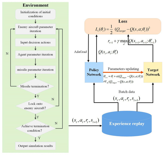
Figure 5. Flowchart of the maneuvering decision training process.

Table 5. DQN training hyperparameters used for BVR maneuvering.

Hyperparameter	Value
Learning rate ($\alpha$)	$5\times {10}^{-4}$
Discount factor ($\gamma$)	$0.99$
Soft update coefficient ($\tau$)	$0.005$
$ϵ$-greedy (initial)	$1.0$
$ϵ$ (final)	$0.01$
$ϵ$ decay	$1\times {10}^{-4}$
Hidden layers	$[400,300]$
Batch size	256
Replay buffer size	$10,000$
Total training epochs	$30,000$

The training process involves using the $ϵ$-greedy [31] policy for action selection, updating the network with the DQN aerial engagement decision framework, and updating the ($s,a,r,s^{\prime }$) tuples in the replay memory to realize the parameter updates of the DQN network. Given the initial position, the action selection and state transition are carried out using the reinforcement learning framework, with the aerial engagement data being generated during the training process.

Therefore, the DQN agent relies solely on the experience data generated by the BVR aerial engagement environment and stored in the experience pool [32] and the designed reward function, without any prior knowledge, to find effective maneuver strategies through training.

4. Results

4.1. Initial Scenario Configuration

The aerial maneuvering decision-making cycle is set to 90 s, with a computational time step of 0.2 s. The initial states of the agent aircraft, designated target aircraft, and interceptor vehicle are fixed as shown in Table 6, following these assumptions: (a) the agent aircraft, designated target aircraft, and dynamic aerial obstacle are on a head-on collision course relative to each other; (b) the dynamic aerial obstacle has completed its acceleration phase and maintains unpowered flight; (c) the designated target aircraft maintains constant horizontal straight flight.

Table 6. Initial State Parameters.

Air Vehicle	Spatial Coordinates	Flight Path Angle	Flight Path Heading	Velocity
Agent	$C_t=(0,35,000,8000)$	${\theta }_t=0°$	${\psi }_t=-90°$	$200\mathrm{m}/\mathrm{s}$
Target Aircraft	$C_e=(0,2300,8000)$	${\theta }_e=0°$	${\psi }_e=90°$	$230\mathrm{m}/\mathrm{s}$
Interceptor	$C_m=(0,5000,8000)$	${\theta }_m=0°$	${\psi }_m=90°$	$1000\mathrm{m}/\mathrm{s}$

The agent’s mission success is determined by the relative speed between the interceptor and the agent, as well as the relative bearing of the target aircraft to the agent. Based on the above assumptions and parameter settings, a simulation is conducted using the DQN aerial engagement decision-making framework.

4.2. Network Training Performance

To evaluate the learning behavior of the proposed DQN framework, Figure 6a,b show the evolution of the training loss and average reward over episodes. The loss curve exhibits a clear decreasing trend and stabilizes after approximately 300 episodes, indicating convergence of the value function. After 3000 episodes, the loss remains stably at 0.05 ± 0.01 with a fluctuation amplitude < 5%, so subsequent data (3000~30,000 episodes) are not displayed. The mean loss value of 0.05 ± 0.01 for 3000~30,000 episodes is supplemented to verify long-term stability. Meanwhile, the average reward steadily increases and reaches a plateau, reflecting that the agent has learned a stable and effective maneuver policy. After 10,000 episodes, the average reward stabilizes at 85 ± 3 with a fluctuation amplitude < 3%, so only data from the key generalization phase (300~10,000 episodes) are displayed. The mean value and fluctuation range of the average reward over 30,000 episodes (85 ± 3) are supplemented to verify long-term stability. These results verify that the proposed DQN achieves good training stability and learning efficiency, forming a reliable basis for subsequent BVR maneuvering mission decision analysis.

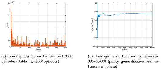
Figure 6. Training performance of the DQN network.

4.3. Simulation Test Results

Based on the parameters and simulation scenario settings, the simulation training for interceptor evasion and target reacquisition was completed. The obtained results were subjected to the following simulation tests under multiple initial conditions to assess the generalization ability of the trained agent.

The engagement trajectories and corresponding key parameter variations for all test scenarios are consolidated in Figure 7 and Figure 8, respectively. Each scenario differs in initial geometry or flight state, representing various threat levels and engagement configurations.

Figure 7. Consolidated 3D and vertical-plane (YZ) trajectories across the four test scenarios. The DQN-trained agent consistently executes coordinated turn-and-climb/dive maneuvers to evade the interceptor and regain target lock under different initial geometries.

Figure 8. Consolidated proximity-rate, energy, and relative-azimuth variations across all four test scenarios. Panels (a,d,g,j) show the decreasing proximity rate $\dot{r}$, indicating interceptor energy depletion; panels (b,e,h,k) depict the energy variation curve of the interceptor; panels (c,f,i,l) depict the azimuth evolution, where maintaining the angle within the radar detection window for more than 1 s confirms successful target reacquisition. Consistent convergence patterns across Scenarios 1–4 demonstrate the generalization and robustness of the trained DQN policy.

To ensure clarity and reproducibility of the evaluation, the performance metrics used in this study are defined as follows:

Evade Success Rate: The proportion of test episodes in which the aircraft successfully avoids the incoming interceptor threat.

Turn Success Rate: Among the episodes where interceptor evasion is successful, the proportion in which the aircraft subsequently re-establishes radar lock on the target.

Average Miss Distance: The relative separation between the aircraft and the interceptor at the moment the interceptor becomes non-lethal (termination conditions 3 or 4), averaged across episodes.

Average Maneuver Time: The elapsed time from interceptor launch to episode termination (success or failure), averaged over test episodes.

Average Energy Used: The mean energy expenditure of the aircraft during the maneuvering process.

4.3.1. Simulation Test Scenario 1

In the initial test (Scenario 1), where the setup matched the training configuration, the DQN-trained agent executed a coordinated large-radius turn in the $X=0$ plane to place the interceptor behind the aircraft. We assume the interceptor is in a powerless flight phase (thrust zero). Based on the interceptor’s kinematics and dynamics, it is constantly affected by drag throughout its flight, causing its speed to continuously decrease. When the evasive agent’s speed exceeds the interceptor’s speed, in principle, the interceptor cannot catch up with the aircraft. The proximity rate $\dot{r}$ reaches zero at approximately 50 s, indicating interceptor energy depletion. This means the interceptor can no longer approach the agent aircraft; therefore, a zero approach rate means the agent aircraft has successfully evaded the interceptor. Concurrently, the relative azimuth remains within the radar detection window for over 1 s (40–50 s), confirming successful target reacquisition. These dynamics are reflected in Figure 7 and Figure 8, demonstrating the learned “evade–relock” maneuver.

4.3.2. Simulation Test Scenario 2

In Scenario 2, the agent starts closer to the incoming interceptor and at a lower altitude ($C_t(0,30,000,7000)$), increasing the threat level. Despite these harsher conditions, the agent adopts a more aggressive low-altitude turning strategy that accelerates interceptor energy loss. The azimuth variation in Figure 8 shows a delayed but stable convergence, indicating that the agent still successfully reacquires the target within the mission time.

4.3.3. Simulation Test Scenario 3

Scenario 3 begins with a positive flight-path angle (${\theta }_t=30°$), making it more difficult to position the interceptor behind via a simple horizontal turn. The agent performs a diving-turn maneuver—descending to convert potential energy into kinetic energy—and then pulls up to complete reorientation. This dive–climb pattern, evident in Figure 7, enables the agent to evade the interceptor while regaining radar lock, validating its adaptability to vertical-motion engagements.

4.3.4. Simulation Test Scenario 4

In Scenario 4, the engagement is not head-on (initial coordinates $C_t(-1000,30,000,7000)$), challenging the agent’s ability to evade while re-aligning the azimuth to the target. The consolidated trajectories (Figure 7) and azimuth traces (Figure 8) show that the agent compensates for the initial bearing offset through asymmetric turning and roll recovery maneuvers, ultimately re-locking onto the target within one minute.

In the initial states of Simulation Test Scenarios 2 to 4, the interceptor threat is heightened, and the task difficulty is increased compared to the training scenarios. Observing the experimental results from Figure 7 and Figure 8, it is evident that despite the increased task difficulty, the intelligent agent model trained using the DQN algorithm continues to adopt similar maneuvering strategies. The agent effectively evades incoming interceptors and reacquires the target aircraft within 1 min, fulfilling the mission requirements. Therefore, the evasion decisions derived from the DQN algorithm demonstrate significant generalization capability.

4.4. Comparison with Baselines

To evaluate the effectiveness of the proposed DQN-based method for aerial engagement evasive maneuvering, we conducted a comparative study against two baseline algorithms: Q-Learning and DDPG. The evaluation metrics include evade success rate, turn success rate, average miss distance, average maneuver time, and average energy used. The results, presented in Table 7, demonstrate that the DQN method consistently outperforms the baseline approaches across all key performance indicators.

Table 7. Quantitative results compared with two baseline methods.

Methods	Evade Success Rate (%, ↑)	Turn Success Rate (%, ↑)	Average Miss Distance (m, ↑)	Average Maneuver Time (s, ↓)	Average Energy Used (J, ↓)	Statistical Test (Evade Success)	95% Confidence Interval (Evade Success)
DQN	97.28	98.31	2355.28	26.62	100.08	p-value = 0.002 t-stat = 3.45	(96.90, 97.66)
Q-Learning	85.63	87.4	753.85	39.64	312.37		(85.00, 86.10)
DDPG	88.59	91.25	253.76	32.39	157.88		(88.00, 89.00)

Note: 1. ↑ indicates that the higher the index value, the better the performance; ↓ indicates that the lower the index value, the better the performance. 2. Bold values represent the optimal results for each evaluation index.

Specifically, DQN achieves the highest evade success rate and turn success rate at 97.28% and 98.31%, respectively, substantially surpassing Q-Learning (85.63%, 87.4%) and DDPG (88.59%, 91.25%). This indicates that DQN is more effective in learning both evasive strategies and turning maneuvers under threat scenarios. In terms of average miss distance, DQN records a significantly larger value (2355.28 m) compared to Q-Learning (753.85 m) and DDPG (253.76 m), suggesting that DQN enables the agent to evade threats at a greater distance, thereby enhancing survivability. Moreover, DQN demonstrates superior maneuver efficiency, with the lowest average maneuver time of 26.62 s, indicating faster evasive responses. Additionally, DQN consumes the least energy (100.08 J), significantly lower than that of Q-Learning (312.37 J) and DDPG (157.88 J), reflecting its energy-efficient decision-making.

In summary, the proposed DQN-based approach exhibits clear advantages in evasive performance, maneuver efficiency, and energy consumption, validating its effectiveness and applicability in dynamic aerial engagement scenarios.

5. Discussion

5.1. Reasons for DQN Superiority

Compared with traditional Q-learning and continuous-action algorithms such as DDPG, the proposed DQN framework shows higher stability and convergence in discrete-action BVR combat scenarios. Its discrete action representation matches the quantized control commands (e.g., load factor and roll angle) of fighter aircraft. In contrast, DDPG’s continuous updates are more sensitive to non-linear and discontinuous rewards. Moreover, DQN’s experience replay and target network help decorrelate samples and enhance generalization.

5.2. Implications for Real-World Deployment

The learned DQN policy demonstrates the potential for autonomous tactical maneuvering that integrates interceptor evasion and re-engagement. For real-world deployment, transferring the trained policy to flight hardware requires: (1) higher-fidelity aerodynamic and sensor models; (2) domain randomization or transfer learning to reduce the simulation–reality gap; and (3) integration within human–AI cooperative control frameworks.

To mitigate these gaps and support future transfer to real flight platforms, a staged sim-to-real strategy is planned. Domain randomization will be applied during training by perturbing key aerodynamic and guidance parameters (e.g., load-factor limits, thrust and drag coefficients, navigation constants) and injecting Gaussian sensor noise, intermittent signal loss, and representative electronic interference. In parallel, system identification using flight-test or hardware-in-the-loop data will be used to calibrate aerodynamic coefficients and radar-noise characteristics, thereby improving model fidelity. Finally, the policy will be validated through a progressive pipeline—first in randomized high-disturbance simulation, then in hardware-in-the-loop setups with real flight-control computers and radar simulators, and ultimately in controlled flight experiments.

5.3. Potential Risks and Limitations

Despite strong performance in simulation, several risks remain. Simplified dynamics and ideal radar assumptions may cause overfitting to the training environment. Real-time onboard computation also poses a constraint, requiring model compression or hardware acceleration. In addition, autonomous decision systems raise safety and ethical concerns that warrant further investigation. Beyond these general risks, the simplified assumptions adopted in this work introduce several concrete limitations that should be acknowledged. First, both the aircraft and interceptor are modeled as point masses, neglecting attitude–coupling effects, control-surface efficiency variations, and structural load constraints. This simplification can lead to discrepancies between the simulated maneuverability and that of real fighter aircraft. Second, the radar model assumes a noise-free and interference-free environment with a deterministic 1 s locking rule, which does not reflect measurement errors, jamming effects, or the more complex lock-on logic found in operational sensors. Third, the simulation–reality gap remains non-trivial: the current environment does not include atmospheric disturbances, sensor noise, or stochastic engagement conditions, all of which may affect the reliability of the learned policy when deployed on real platforms.

Overall, DQN provides a promising foundation for intelligent maneuver decision-making, while bridging the gap between simulation and operational deployment remains an open research challenge. Future work will incorporate aircraft-specific physical constraints, including actuator rate/lag limits and angle-of-attack restrictions, to construct a higher-fidelity control environment and enable engineering-level validation.

6. Conclusions

This paper presents a DQN-based framework for autonomous maneuver decision-making in BVR aerial engagements, focusing on interceptor evasion and target re-engagement tasks. A model-free DQN approach replaces rule-based or model-dependent traditional methods, improving adaptability to complex dynamic environments and reducing manual engineering efforts. For discrete-action BVR tasks, the framework integrates scenario-specific state representation and action space design, achieving better training stability and decision performance than Q-Learning and DDPG. A hybrid reward structure accelerates learning, enabling the agent to autonomously acquire effective strategies from simulation data without prior knowledge. Validation shows the trained agent successfully evades interceptors, reacquires targets, reduces maneuver time, and generalizes across challenging scenarios advancing BVR maneuver planning for robust aerial engagement systems. Idealized dynamics modeling assumptions common in aerial engagement simulation may limit real-world applicability under complex aerodynamic and environmental conditions, affecting policy transfer fidelity. Future work will explore more complex BVR aerial engag ement scenarios and integrate higher-fidelity models (e.g., 6-degree-of-freedom (6-DOF) aircraft dynamic model, realistic aerodynamic effects and sensor noise) to enhance strategy robustness, bridging simulation and real-world deployment. In practical applications, the proposed framework can serve either as a decision-support tool to assist human pilots or as an autonomous maneuver planning module for UAVs, depending on the level of human–AI integration.

References

- Yang, X.; Yuan, F.; Wu, M.; Tu, J.; Ye, X.; Dong, Y. Knowledge-Driven Target Trajectory Prediction Method for BVR Air Game Mission. In 2024 China Automation Congress (CAC); IEEE: Piscataway, NJ, USA, 2024; pp. 1976–1981. [Google Scholar]
- Shinar, J.; Guelman, M.; Silberman, G.; Green, A. On Optimal missile avoidance—A comparison between optimal control and differential game solutions. In Proceedings. ICCON IEEE International Conference on Control and Applications; IEEE: Piscataway, NJ, USA, 1989; pp. 453–459. [Google Scholar]
- Liao, S.H. Expert system methodologies and applications—A decade review from 1995 to 2004. Expert Syst. Appl. 2005, 28, 93–103. [Google Scholar] [CrossRef]
- Sridharan, M. Short review on various applications of fuzzy logic-based expert systems in the field of solar energy. Int. J. Ambient Energy 2022, 43, 5112–5128. [Google Scholar]
- Lian, B.; Donge, V.S.; Lewis, F.L.; Chai, T.; Davoudi, A. Data-Driven Inverse Reinforcement Learning Control for Linear Multiplayer Games. IEEE Trans. Neural Netw. Learn. Syst. 2024, 35, 2028–2041. [Google Scholar]
- Zaliskyi, M.; Yashanov, I.; Okoro, O.C.; Shcherbyna, O. Analysis of Learning Efficiency of Expert System for Decision-Making Support in Aviation. In 2022 12th International Conference on Advanced Computer Information Technologies (ACIT); IEEE: Piscataway, NJ, USA, 2022; pp. 172–175. [Google Scholar]
- Tao, Y.; Lina, G.; Mingkuan, D.; Ke, Z.; Xiaoma, L. Research on the evasive strategy of missile based on the theory of differential game. In 2015 34th Chinese Control Conference (CCC); IEEE: Piscataway, NJ, USA, 2015; pp. 5182–5187. [Google Scholar]
- Turetsky, V.; Shima, T. Hybrid evasion strategy against a missile with guidance law of variable structure. In 2016 American Control Conference (ACC); IEEE: Piscataway, NJ, USA, 2016; pp. 3132–3137. [Google Scholar]
- Garcia, E.; Casbeer, D.W.; Pachter, M. Active target defence differential game: Fast defender case. IET Control Theory Appl. 2017, 11, 2985–2993. [Google Scholar] [CrossRef]
- Qi, D.; Li, L.; Xu, H.; Tian, Y.; Zhao, H. Modeling and solving of the missile pursuit-evasion game problem. In 2021 40th Chinese Control Conference (CCC); IEEE: Piscataway, NJ, USA, 2021; pp. 1526–1531. [Google Scholar]
- Karelahti, J.; Virtanen, K.; Raivio, T. Near-optimal missile avoidance trajectories via receding horizon control. J. Guid. Control Dyn. 2007, 30, 1287–1298. [Google Scholar] [CrossRef]
- Imado, F.; Kuroda, T. Family of local solutions in a missile-aircraft differential game. J. Guid. Control Dyn. 2011, 34, 583–591. [Google Scholar] [CrossRef]
- Shima, T. Optimal cooperative pursuit and evasion strategies against a homing missile. J. Guid. Control Dyn. 2011, 34, 414–425. [Google Scholar] [CrossRef]
- Bao, X.; Jiang, C. Time-Optimal Control Algorithm of Aircraft Maneuver. In Advances in Guidance, Navigation and Control; Springer: Singapore, 2022; pp. 4683–4691. [Google Scholar]
- Zhang, X.; Guo, H.; Yan, T.; Wang, X.; Sun, W.; Fu, W.; Yan, J. Penetration Strategy for High-Speed Unmanned Aerial Vehicles: A Memory-Based Deep Reinforcement Learning Approach. Drones 2024, 8, 275. [Google Scholar] [CrossRef]
- Kasumba, H.; Kunisch, K. On computation of the shape Hessian of the cost functional without shape sensitivity of the state variable. J. Optim. Theory Appl. 2014, 162, 779–804. [Google Scholar] [CrossRef]
- Li, Y. Deep reinforcement learning: An overview. arXiv 2017, arXiv:1701.07274. [Google Scholar]
- AlMahamid, F.; Grolinger, K. Autonomous unmanned aerial vehicle navigation using reinforcement learning: A systematic review. Eng. Appl. Artif. Intell. 2022, 115, 105321. [Google Scholar] [CrossRef]
- Wang, D.; Zhang, J.; Yang, Q.; Liu, J.; Shi, G.; Zhang, Y. An Autonomous Attack Decision-Making Method Based on Hierarchical Virtual Bayesian Reinforcement Learning. IEEE Trans. Aerosp. Electron. Syst. 2024, 60, 7075–7088. [Google Scholar] [CrossRef]
- Keong, C.W.; Shin, H.S.; Tsourdos, A. Reinforcement Learning for Autonomous Aircraft Avoidance. In 2019 Workshop on Research, Education and Development of Unmanned Aerial Systems (RED UAS); IEEE: Piscataway, NJ, USA, 2019; pp. 126–131. [Google Scholar]
- Fan, X.; Li, D.; Zhang, W.; Wang, J.; Guo, J. Missile evasion decision training based on deep reinforcement learning. Electron. Opt. Control 2021, 28, 81–85. [Google Scholar]
- Wang, Y.; Ren, T.; Fan, Z. Autonomous maneuver decision of UAV based on deep reinforcement learning: Comparison of DQN and DDPG. In 2022 34th Chinese Control and Decision Conference (CCDC); IEEE: Piscataway, NJ, USA, 2022; pp. 4857–4860. [Google Scholar]
- Özbek, M.M.; Koyuncu, E. Missile Evasion Maneuver Generation with Model-free Deep Reinforcement Learning. In 2023 10th International Conference on Recent Advances in Air and Space Technologies (RAST); IEEE: Piscataway, NJ, USA, 2023; pp. 1–6. [Google Scholar]
- Imado, F.; Heike, Y.; Kinoshita, T. Research on a new aircraft point-mass model. J. Aircr. 2011, 48, 1121–1130. [Google Scholar] [CrossRef]
- Wei, Y.; Zhang, H.; Wang, Y.; Huang, C. Autonomous maneuver decision-making through curriculum learning and reinforcement learning with sparse rewards. IEEE Access 2023, 11, 73543–73555. [Google Scholar] [CrossRef]
- Shaferman, V.; Shima, T. Cooperative multiple-model adaptive guidance for an aircraft defending missile. J. Guid. Control. Dyn. 2010, 33, 1801–1813. [Google Scholar] [CrossRef]
- Zhang, H.; Zhou, H.; Wei, Y.; Huang, C. Autonomous maneuver decision-making method based on reinforcement learning and Monte Carlo tree search. Front. Neurorobotics 2022, 16, 996412. [Google Scholar] [CrossRef]
- Zhu, L.J.; Cai, Y.; Tong, K.W.; Wu, S.; Xiang, F.; Duan, Y.; Hou, Y.; Zhu, G.; Wu, E.Q. Adaptive Guidance in Dynamic Environments: A Deep Reinforcement Learning Approach for Highly Maneuvering Targets. IEEE Trans. Comput. Soc. Syst. 2025, 12, 3537–3547. [Google Scholar] [CrossRef]
- Wang, C.; Wang, J.; Wang, J.; Zhang, X. Deep-Reinforcement-Learning-Based Autonomous UAV Navigation with Sparse Rewards. IEEE Internet Things J. 2020, 7, 6180–6190. [Google Scholar] [CrossRef]
- Gao, M.; Yan, T.; Li, Q.; Fu, W.; Zhang, J. Intelligent pursuit–evasion game based on deep reinforcement learning for hypersonic vehicles. Aerospace 2023, 10, 86. [Google Scholar] [CrossRef]
- Liu, F.; Viano, L.; Cevher, V. Understanding deep neural function approximation in reinforcement learning via ϵ-greedy exploration. Adv. Neural Inf. Process. Syst. 2022, 35, 5093–5108. [Google Scholar]
- Lv, L.; Zhang, S.; Ding, D.; Wang, Y. Path planning via an improved DQN-based learning policy. IEEE Access 2019, 7, 67319–67330. [Google Scholar] [CrossRef]
Disclaimer/Publisher’s Note: The statements, opinions and data contained in all publications are solely those of the individual author(s) and contributor(s) and not of MDPI and/or the editor(s). MDPI and/or the editor(s) disclaim responsibility for any injury to people or property resulting from any ideas, methods, instructions or products referred to in the content. |
© 2026 by the authors. Licensee MDPI, Basel, Switzerland. This article is an open access article distributed under the terms and conditions of the Creative Commons Attribution (CC BY) license.